Convergence of a finite-volume scheme for a degenerate-singular cross-diffusion system
for biofilms

Abstract.

An implicit Euler finite-volume scheme for a cross-diffusion system modeling biofilm growth is analyzed by exploiting its formal gradient-flow structure. The numerical scheme is based on a two-point flux approximation that preserves the entropy structure of the continuous model. Assuming equal diffusivities, the existence of nonnegative and bounded solutions to the scheme and its convergence are proved. Finally, we supplement the study by numerical experiments in one and two space dimensions.

1. Introduction

Biofilms are organized, cooperating communities of microorganisms. They can be used for the treatment of wastewater [10, 20], as they help to reduce sulfate and to remove nitrogen. Typically, biofilms consist of several species such that multicomponent fluid models need to be considered. Recently, a multi-species biofilm model was introduced by Rahman, Sudarsan, and Eberl [22], which reflects the same properties as the single-species diffusion model of [14]. The model has a porous-medium-type degeneracy when the local biomass vanishes, and a singularity when the biomass reaches the maximum capacity, which guarantees the boundedness of the total mass. The model was derived formally from a space-time discrete walk on a lattice in [22]. The global existence of weak solutions to the single-species model was proved in [15], while the global existence analysis for the multi-species cross-diffusion system can be found in [13]. The proof of the multi-species model is based on an entropy method which also provides the boundedness of the biomass hidden in its entropy structure. Numerical simulations were performed in [13, 22], but no numerical analysis was given. In this paper, we analyze an implicit Euler finite-volume scheme of the multi-species system that preserves the structure of the continuous model, namely positivity, boundedness, and discrete entropy production.

The model equations for the proportions of the biofilm species $u_{i}$ are given by

(1) $$\partial_{t}u_{i}+\operatorname{div}{\mathcal{F}}_{i}=0,\quad{\mathcal{F}}_{i}=-\alpha_{i}p(M)^{2}\nabla\frac{u_{i}q(M)}{p(M)}\quad\mbox{in }\Omega,\ t>0,\ i=1,\ldots,n,$$

where $\Omega\subset{\mathbb{R}}^{d}$ ($d\geq 1$) is a bounded domain, $\alpha_{i}>0$ are some diffusion coefficients, and $M=\sum_{i=1}^{n}u_{i}$ is the total biomass. The proportions $u_{i}(x,t)$ are nonnegative and satisfy $M\leq 1$. We have assumed for simplicity that the functions $p$ and $q$ only depend on the total biomass and are the same for all species. The function $p\in C^{1}([0,1])$ is decreasing and satisfies $p(1)=0$, and $q$ is defined by

(2) $$q(M):=\frac{p(M)}{M}\int_{0}^{M}\frac{s^{a}}{(1-s)^{b}}\frac{ds}{p(s)^{2}},\quad M>0,$$

where $a$, $b\geq 1$. Equations (1) are complemented by initial and mixed boundary conditions:

(3) $$u_{i}(0)=u_{i}^{0}\quad\mbox{in }\Omega,\ i=1,\ldots,n,$$

(4) $$u_{i}=u_{i}^{D}\quad\mbox{on }\Gamma^{D},\quad\nabla{\mathcal{F}}_{i}\cdot\nu=0\quad\mbox{on }\Gamma^{N},$$

where $\Gamma^{D}$ is the contact boundary part, $\Gamma^{N}$ is the union of isolating boundary parts, and $\partial\Omega=\Gamma^{D}\cup\Gamma^{N}$.

We recover the single-species model if all species are the same and all diffusivities $\alpha_{i}$ are equal, $\alpha_{i}=1$ for $i=1,\ldots,n$. Indeed, summing (1) over $i=1,\ldots,n$, it follows that

(5) $$\partial_{t}M=\operatorname{div}\bigg{(}p(M)^{2}\nabla\frac{Mq(M)}{p(M)}\bigg{)}=\operatorname{div}\bigg{(}\frac{M^{a}}{(1-M)^{b}}\nabla M\bigg{)},$$

which makes the degenerate-singular structure of the model evident.

Equations (1) can be written as the cross-diffusion system

(6) $$\partial_{t}u_{i}-\operatorname{div}\bigg{(}\sum_{j=1}^{n}A_{ij}(u)\nabla u_{j}\bigg{)}=0\quad\mbox{in }\Omega,\ t>0,$$

where the nonlinear diffusion coefficients are defined by

(7) $$A_{ij}(u)=\alpha_{i}\delta_{ij}p(M)q(M)+\alpha_{i}u_{i}\big{(}p(M)q^{\prime}(M)-p^{\prime}(M)q(M)\big{)},\quad i,j=1,\ldots,n.$$

Due to the cross-diffusion structure, standard techniques like the maximum principle and regularity theory cannot be used. Moreover, the diffusion matrix $(A_{ij}(u))$ is generally neither symmetric nor positive definite.

The key of the analysis, already observed in [13], is that system (6)-(7) allows for an entropy or formal gradient-flow structure. Indeed, introduce the (relative) entropy

$$H(u)=\int_{\Omega}h^{*}(u|u^{D})dx,\quad\mbox{where}$$

$$h^{*}(u|u^{D})=h(u)-h(u^{D})-h^{\prime}(u^{D})\cdot(u-u^{D}),$$

$$h(u)=\sum_{i=1}^{n}\big{(}u_{i}(\log u_{i}-1)+1\big{)}+\int_{0}^{M}\log\frac{q(s)}{p(s)}ds,$$

defined on the set

(8) $${\mathcal{O}}=\bigg{\{}u=(u_{1},\ldots,u_{n})\in(0,\infty)^{n}:\sum_{i=1}^{n}u_{i}<1\bigg{\}}.$$

A computation gives the entropy identity [13, Theorem 2.1]

(9) $$\frac{dH}{dt}+2\sum_{i=1}^{n}\alpha_{i}\int_{\Omega}p(M)^{2}\bigg{|}\nabla\sqrt{\frac{u_{i}q(M)}{p(M)}}\bigg{|}^{2}dx=0.$$

Thus, $H$ is a Lyapunov functional along the solutions to (1). Moreover, under some assumptions on $p$, the entropy production term (the second term on the left-hand side) can be bounded from below, for some constant $C>0$, by

$$\sum_{i=1}^{n} \alpha_{i}\int_{\Omega}p(M)^{2}\bigg{|}\nabla\sqrt{\frac{u_{i}q(M)}{p(M)}}\bigg{|}^{2}dx$$

(10) $$\geq C\int_{\Omega}\frac{M^{a-1}|\nabla M|^{2}}{(1-M)^{1+b+\kappa}}dx+\sum_{i=1}^{n}\int_{\Omega}p(M)q(M)|\nabla\sqrt{u_{i}}|^{2}dx,$$

yielding suitable gradient estimates. Moreover, it implies that $(1-M)^{1-b-\kappa}$ is integrable, showing that $M<1$ a.e. in $\Omega$, $t>0$, which excludes biofilm saturation and allows us to define the nonlinear terms.

Another feature of the entropy method is that equations (1), written in the so-called entropy variables $w_{i}=\partial h^{*}/\partial u_{i}$, can be written as the formal gradient-flow system

$$\partial_{t}u-\operatorname{div}(B(w)\nabla w)=0,$$

with a positive semidefinite diffusion matrix $B$. Since the derivative $(h^{*})^{\prime}:{\mathcal{O}}\to{\mathbb{R}}^{n}$ is invertible [13, Lemma 3.3], $u$ can be interpreted as a function of $w$, $u(w)=[(h^{*})^{\prime}]^{-1}(w)$, mapping ${\mathbb{R}}^{n}$ to ${\mathcal{O}}$. This gives automatically $u(w)\in{\mathcal{O}}$ and consequently $L^{\infty}$ bounds. This property, for another volume-filling model, was first observed in [8] and later generalized in [17].

The aim of this paper is to reproduce the above-mentioned properties on the discrete level. For this, we suggest an implicit Euler scheme in time (with time step size $\Delta t$) and a finite-volume discretization in space (with grid size parameter $\Delta x$), based on two-point approximations. The challenge is to formulate the discrete fluxes such that the scheme preserves the entropy structure of the model and to design the fluxes such that we are able to establish the upper bound $M<1$ a.e. in $\Omega$, $t>0$. We suggest the discrete fluxes (20), where the coefficient $p(M)^{2}$ is replaced by $(p(M_{K})^{2}+p(M_{L})^{2})/2$, and $K$ and $L$ are two neighboring control volumes with a common edge (see Section 2.1 for details). We establish a discrete counterpart of (10) in Lemma 4.3. This result is proved by exploiting the properties of the functions $p$ and $q$ as in [13, Lemma 3.4] and distinguishing carefully the cases $M\leq 1-\delta$ and $M>1-\delta$ for sufficiently small $\delta>0$. However, due to the lack of a chain rule at the discrete level, we cannot conclude that the “discrete” biomass satisfies $M<1$. To overcome this issue, we need to assume that the diffusivities are all equal. Then, summing the finite-volume analog of (1) over $i=1,\ldots,n$, we obtain a discrete analog of the diffusion equation (5) for $M$ that allows us to apply a discrete maximum principle, leading to $M<1$.

Our results can be sketched as follows (see Section 2.3 for the precise statements):

• We prove the existence of finite-volume solutions with nonnegative discrete proportions $u_{i,K}$ and discrete total biomass $M_{K}<1$ for all control volumes $K$.

• The discrete solution satisfies a discrete analog of the entropy equality (which becomes an inequality in (25)) and of the lower bound (10) for the entropy production.

• The discrete solution converges in a certain sense, for mesh sizes $(\Delta x,\Delta t)\to 0$, to a weak solution to (1).

Let us notice that even if the assumption on the diffusion coefficients provides an upper bound for $M$, we cannot establish the nonnegativity of the densities $u_{i}$ by using a maximum principle. Instead, we adapt at the discrete level the so-called boundedness-by-entropy method, introduced in [8] and developed in [17], to a finite-volume scheme. This approach allows us to prove that the solutions to the nonlinear scheme proposed in this paper satisfy the properties (i)-(iii); see Theorems 2.1 and 2.2. The adaptation of this technique represents the main originality of this work.

There are several finite-volume schemes for other cross-diffusion systems in the mathematical literature. For instance, an upwind two-point flux approximation was used in [1] for a seawater intrusion model. A positivity-preserving two-point flux approximation for a two-species population system was suggested in [4]. The Laplacian structure of the population model was exploited in [19] to design a convergent linear finite-volume scheme, avoiding fully implicit approximations. Cross-diffusion systems with nonlocal (in space) terms modeling food chains and epidemics were approximated in [2, 3]. The convergence of the finite-volume scheme of a degenerate cross-diffusion system arising in ion transport was shown in [9], and the existence of a finite-volume scheme for a population cross-diffusion system was proved in [18].

A finite-volume scheme for the biofilm growth, coupled with the computation of the surrounding fluid flow, was presented in [24]. Finite-volume-based simulations of biofilm processes in axisymmetric reactors were given in [23]. Closer to our numerical study is the work [21], where the single-species biofilm model was discretized using finite volumes, but without any numerical analysis. In this paper, we prove the existence of discrete solutions and the convergence of the finite-volume scheme for (1) for the first time.

The paper is organized as follows. The notation and assumptions on the mesh as well as the main theorems are introduced in Section 2. The existence of discrete solutions is proved in Section 3, based on a topological degree argument. We show a gradient estimate, an estimate of the discrete time derivative, and the lower bound for the entropy production in Section 4. These estimates allow us in Section 5 to apply the discrete compactness argument in [5] to conclude the a.e. convergence of the proportions and to show the convergence of the discrete gradient associated to $\nabla(u_{i}q(M)/p(M))$. The convergence of the scheme is then proved in Section 6. In Section 7, we present some numerical results in one and two space dimensions. They illustrate the $L^{2}$-convergence rate in space of the numerical scheme and show the convergence of the solutions to the steady states.

2. Numerical scheme and main results

In this section, we introduce the numerical scheme and detail our main results.

2.1. Notation and assumptions

Let $\Omega\subset{\mathbb{R}}^{2}$ be an open, bounded, polygonal domain with $\partial\Omega=\Gamma^{D}\cup\Gamma^{N}\in C^{0,1}$, $\Gamma^{D}\cap\Gamma^{N}=\emptyset$, and $\operatorname{meas}(\Gamma^{D})>0$. We consider only two-dimensional domains $\Omega$, but the generalization to higher dimensions is straightforward. An admissible mesh ${\mathcal{M}}=({\mathcal{T}},{\mathcal{E}},{\mathcal{P}})$ of $\Omega$ is given by a family ${\mathcal{T}}$ of open polygonal control volumes (or cells), a family ${\mathcal{E}}$ of edges, and a family ${\mathcal{P}}$ of points $(x_{K})_{K\in{\mathcal{T}}}$ associated to the control volumes and satisfying Definition 9.1 in [16]. This definition implies that the straight line between two centers of neighboring cells $\overline{x_{K}x_{L}}$ is orthogonal to the edge $\sigma=K|L$ between two cells $K$ and $L$. The condition is satisfied by, for instance, triangular meshes whose triangles have angles smaller than $\pi/2$ [16, Examples 9.1] or Voronoï meshes [16, Example 9.2].

The family of edges ${\mathcal{E}}$ is assumed to consist of the interior edges $\sigma\in{\mathcal{E}}_{\rm int}$ satisfying $\sigma\in\Omega$ and the boundary edges $\sigma\in{\mathcal{E}}_{\rm ext}$ fulfilling $\sigma\subset\partial\Omega$. We suppose that each exterior edge is an element of either the Dirichlet or Neumann boundary, i.e. ${\mathcal{E}}_{\rm ext}={\mathcal{E}}_{\rm ext}^{D}\cup{\mathcal{E}}_{\rm ext}^{N}$. For a given control volume $K\in{\mathcal{T}}$, we denote by ${\mathcal{E}}_{K}$ the set of its edges. This set splits into ${\mathcal{E}}_{K}={\mathcal{E}}_{{\rm int},K}\cup{\mathcal{E}}_{{\rm ext},K}^{D}\cup{\mathcal{E}}_{{\rm ext},K}^{N}$. For any $\sigma\in{\mathcal{E}}$, there exists at least one cell $K\in{\mathcal{T}}$ such that $\sigma\in{\mathcal{E}}_{K}$. We denote this cell by $K_{\sigma}$. When $\sigma$ is an interior cell, $\sigma=K|L$, $K_{\sigma}$ can be either $K$ or $L$.

Let $\sigma\in{\mathcal{E}}$ be an edge. We define

$${\mathrm{d}}_{\sigma}=\left\{\begin{array}[]{ll}{\mathrm{d}}(x_{K},x_{L})&\quad\mbox{if }\sigma=K|L\in{\mathcal{E}}_{{\rm int}},\\ {\mathrm{d}}(x_{K},\sigma)&\quad\mbox{if }\sigma\in{\mathcal{E}}_{{\rm ext},K},\end{array}\right.$$

where d is the Euclidean distance in ${\mathbb{R}}^{2}$. The transmissibility coefficient is defined by

(11) $$\tau_{\sigma}=\frac{{\mathrm{m}}(\sigma)}{{\mathrm{d}}_{\sigma}},$$

where ${\mathrm{m}}(\sigma)$ denotes the Lebesgue measure of $\sigma$. We assume that the mesh satisfies the following regularity requirement: There exists $\xi>0$ such that

(12) $${\mathrm{d}}(x_{K},\sigma)\geq\xi{\mathrm{d}}_{\sigma}\quad\mbox{for all }K\in{\mathcal{T}},\ \sigma\in{\mathcal{E}}_{K}.$$

This hypothesis is needed to apply a discrete Sobolev inequality; see [6].

The size of the mesh is denoted by $\Delta x=\max_{K\in{\mathcal{T}}}\operatorname{diam}(K)$. Let $N_{T}\in{\mathbb{N}}$ be the number of time steps, $\Delta t=T/N_{T}$ be the time step and set $t_{k}=k\Delta t$ for $k=0,\ldots,N_{T}$. We denote by ${\mathcal{D}}$ an admissible space-time discretization of $Q_{T}:=\Omega\times(0,T)$ composed of an admissible mesh ${\mathcal{M}}$ of $\Omega$ and the values $(\Delta t,N_{T})$. The size of ${\mathcal{D}}$ is defined by $\eta:=\max\{\Delta x,\Delta t\}$.

As it is usual for the finite-volume method, we introduce functions that are piecewise constant in space and time. A finite-volume scheme provides a vector $v_{\mathcal{T}}=(v_{K})_{K\in{\mathcal{T}}}\in{\mathbb{R}}^{\#{\mathcal{T}}}$ of approximate values of a function $v$ and the associate piecewise constant function, still denoted by $v_{\mathcal{T}}$,

$$v_{\mathcal{T}}=\sum_{K\in{\mathcal{T}}}v_{K}\mathbf{1}_{K},$$

where $\mathbf{1}_{K}$ is the characteristic function of $K$. The vector $v_{\mathcal{M}}$, containing the approximate values in the control volumes and the approximate values on the Dirichlet boundary edges, is written as $v_{\mathcal{M}}=(v_{\mathcal{T}},v_{{\mathcal{E}}^{D}})$, where $v_{{\mathcal{E}}^{D}}=(v_{\sigma})_{\sigma\in{\mathcal{E}}_{{\rm ext}}^{D}}\in{\mathbb{R}}^{\#{\mathcal{E}}_{\rm ext}^{D}}$. For a vector $v_{\mathcal{M}}$, we introduce for $K\in{\mathcal{T}}$ and $\sigma\in{\mathcal{E}}_{K}$ the notation

(13) $$v_{K,\sigma}=\left\{\begin{array}[]{ll}v_{L}&\quad\mbox{if }\sigma=K|L\in{\mathcal{E}}_{{\rm int},K},\\ v_{\sigma}&\quad\mbox{if }\sigma\in{\mathcal{E}}_{{\rm ext},K}^{D},\\ v_{K}&\quad\mbox{if }\sigma\in{\mathcal{E}}_{{\rm ext},K}^{N}\end{array}\right.$$

and the discrete gradient

(14) $$D_{\sigma}v:=|D_{K,\sigma}v|,\quad\mbox{where }D_{K,\sigma}v=v_{K,\sigma}-v_{K}.$$

The discrete $H^{1}(\Omega)$ seminorm and the (squared) discrete $H^{1}(\Omega)$ norm are then defined by

(15) $$|v_{\mathcal{M}}|_{1,2,{\mathcal{M}}}=\bigg{(}\sum_{\sigma\in{\mathcal{E}}}\tau_{\sigma}(D_{\sigma}v)^{2}\bigg{)}^{1/2},\quad\|v_{\mathcal{M}}\|^{2}_{1,2,{\mathcal{M}}}=\|v_{\mathcal{M}}\|^{2}_{0,2,{\mathcal{M}}}+|v_{\mathcal{M}}|^{2}_{1,2,{\mathcal{M}}},$$

where $\|\cdot\|_{0,p,{\mathcal{M}}}$ denotes the $L^{p}(\Omega)$ norm

$$\|v_{\mathcal{M}}\|_{0,p,{\mathcal{M}}}=\bigg{(}\sum_{K\in{\mathcal{T}}}{\mathrm{m}}(K)|v_{K}|^{p}\bigg{)}^{1/p},\quad\forall 1\leq p<\infty.$$

Thanks to the regularity assumption (12) and the fact that $\Omega$ is two-dimensional, we have

(16) $$\sum_{K\in{\mathcal{T}}}\sum_{\sigma\in{\mathcal{E}}_{K}}{\mathrm{m}}(\sigma){\mathrm{d}}(x_{K},\sigma)\leq 2\sum_{K\in{\mathcal{T}}}{\mathrm{m}}(K)=2{\mathrm{m}}(\Omega).$$

2.2. Numerical scheme

We are now in the position to define the finite-volume discretization of (1)-(4). Let ${\mathcal{D}}$ be a finite-volume discretization of $Q_{T}$. The initial and boundary conditions are discretized by the averages

(17) $$u_{i,K}^{0} =\frac{1}{{\mathrm{m}}(K)}\int_{K}u_{i}^{0}(x)dx\quad\mbox{for }K\in{\mathcal{T}},$$

(18) $$u_{i,\sigma}^{D} =\frac{1}{{\mathrm{m}}(\sigma)}\int_{\sigma}u_{i}^{D}ds\quad\mbox{for }\sigma\in{\mathcal{E}}_{\rm ext}^{D},\ i=1,\ldots,n.$$

We suppose for simplicity that the Dirichlet datum is constant on $\Gamma^{D}$ such that $u_{i,\sigma}^{D}=u_{i}^{D}$ for $i=1,\ldots,n$. Furthermore, we set $u_{i,\sigma}^{k}=u_{i,\sigma}^{D}$ for $\sigma\in{\mathcal{E}}_{\rm ext}^{D}$ at time $t_{k}$.

Let $u_{i,K}^{k}$ be an approximation of the mean value of $u_{i}(\cdot,t_{k})$ in the cell $K$. Then the implicit Euler finite-volume scheme reads as

(19) $$\frac{{\mathrm{m}}(K)}{\Delta t}(u_{i,K}^{k}-u_{i,K}^{k-1})+\sum_{\sigma\in{\mathcal{E}}_{K}}{\mathcal{F}}_{i,K,\sigma}^{k}=0,$$

(20) $${\mathcal{F}}_{i,K,\sigma}^{k}=-\tau_{\sigma}\alpha_{i}(p_{\sigma}^{k})^{2}D_{K,\sigma}\bigg{(}\frac{u_{i}^{k}q(M^{k})}{p(M^{k})}\bigg{)},$$

where $K\in{\mathcal{T}}$, $\sigma\in{\mathcal{E}}_{K}$, $i=1,\ldots,n$, and the value $p_{\sigma}^{k}$ is defined by

(21) $$(p_{\sigma}^{k})^{2}:=\frac{p(M_{K}^{k})^{2}+p(M_{K,\sigma}^{k})^{2}}{2},$$

recalling definition (11) for $\tau_{\sigma}$ and notation (13) for $M^{k}_{K,\sigma}$.

Observe that definitions (13) and (14) ensure that the discrete fluxes vanish on the Neumann boundary edges, i.e. ${\mathcal{F}}_{i,K,\sigma}^{k}=0$ for all $\sigma\in{\mathcal{E}}_{{\rm ext},K}^{N}$, $k\in{\mathbb{N}}$, and $i=1,\ldots,n$. This is consistent with the Neumann boundary conditions in (4).

For the convergence result, we need to define the discrete gradients. To this end, let the vector $u_{\mathcal{M}}=(u_{\mathcal{T}},u_{{\mathcal{E}}^{D}})$ as defined before. Then we introduce the piecewise constant approximation $u_{\mathcal{D}}=(u_{1,{\mathcal{D}}},\ldots,u_{n,{\mathcal{D}}})$ by

(22) $$u_{i,{\mathcal{D}}}(x,t)=\sum_{K\in{\mathcal{T}}}u_{i,K}^{k}\mathbf{1}_{K}(x) \quad\mbox{for }x\in\Omega,\ t\in(t_{k-1},t_{k}],$$

(23) $$u_{i,{\mathcal{D}}}(x,t)=u_{i}^{D} \quad\mbox{for }x\in\Gamma^{D},i=1,\ldots,n.$$

For given $K\in{\mathcal{T}}$ and $\sigma\in{\mathcal{E}}_{K}$, we define the cell $T_{K,\sigma}$ of the dual mesh as follows:

• If $\sigma=K|L\in{\mathcal{E}}_{{\rm int},K}$, then $T_{K,\sigma}$ is that cell (“diamond”) whose vertices are given by $x_{K}$, $x_{L}$, and the end points of the edge $\sigma$.

• If $\sigma\in{\mathcal{E}}_{{\rm ext},K}$, then $T_{K,\sigma}$ is that cell (“triangle”) whose vertices are given by $x_{K}$ and the end points of the edge $\sigma$.

An example of a construction of such a dual mesh can be found in [11]. The cells $T_{K,\sigma}$ define a partition of $\Omega$. The definition of the dual mesh implies the following properties:

• As the straight line between two neighboring centers of cells $\overline{x_{K}x_{L}}$ is orthogonal to the edge $\sigma=K|L$, it follows that

  (24) $${\mathrm{m}}(\sigma){\mathrm{d}}(x_{K},x_{L})=2{\mathrm{m}}(T_{K,\sigma})\quad\mbox{for all }\sigma=K|L\in{\mathcal{E}}_{{\rm int},K}.$$

• The property ${\mathrm{m}}(T_{K,\sigma})={\mathrm{m}}(T_{L,\sigma})$ for $\sigma=K|L\in{\mathcal{E}}_{{\rm int},K}$ implies that

  $$\sum_{\begin{subarray}{c}\sigma\in{\mathcal{E}}\\ K=K_{\sigma}\end{subarray}}{\mathrm{m}}(T_{K,\sigma})\leq 2{\mathrm{m}}(\Omega),$$

  where the sum is over all edges $\sigma\in{\mathcal{E}}$, and to each given $\sigma$ we associate the cell $K=K_{\sigma}$.

We define the approximate gradient of a piecewise constant function $u_{\mathcal{D}}$ in $Q_{T}$ given by (22)-(23) as follows:

$$\nabla^{\mathcal{D}}u_{{\mathcal{D}}}(x,t)=\frac{{\mathrm{m}}(\sigma)}{{\mathrm{m}}(T_{K,\sigma})}D_{K,\sigma}u^{k}\,\nu_{K,\sigma}\quad\mbox{for }x\in T_{K,\sigma},\ t\in(t_{k-1},t_{k}],$$

where the discrete operator $D_{K,\sigma}$ is given in (14) and $\nu_{K,\sigma}$ is the unit vector that is normal to $\sigma$ and points outward of $K$.

2.3. Main results

Our first result guarantees that scheme (17)-(21) possesses a solution and that it preserves the entropy dissipation property. Let us collect our assumptions:

(H4)

Domain: $\Omega\subset{\mathbb{R}}^{2}$ is a bounded polygonal domain with Lipschitz boundary $\partial\Omega=\Gamma^{D}\cup\Gamma^{N}$, $\Gamma^{D}\cap\Gamma^{N}=\emptyset$, and $\operatorname{meas}(\partial\Gamma^{D})>0$.

Discretization: ${\mathcal{D}}$ is an admissible discretization of $Q_{T}$ satisfying the regularity condition (12).

Data: $u^{0}=(u_{1}^{0},\ldots,u_{n}^{0})\in L^{2}(\Omega;[0,\infty)^{n})$ , $u^{D}=(u_{1}^{D},\ldots,u_{n}^{D})\in(0,\infty)^{n}$ is a constant vector, $\sum_{i=1}^{n}u_{i}^{0}<1$ in $\Omega$, $\sum_{i=1}^{n}u^{D}_{i}<1$, and $\alpha_{1},\ldots,\alpha_{n}>0$, $a$, $b\geq 1$.

Functions: $p\in C^{1}([0,1];[0,\infty))$ is decreasing, $p(1)=0$, and there exist $c$, $\kappa>0$ such that $\lim_{M\to 1}(-(1-M)^{1+\kappa}p^{\prime}(M)/p(M))=c$. The function $q$ is defined in (2).

For our main results, we need the following technical assumption:

(A1)

The diffusion constants are equal, $\alpha_{i}=1$ for $i=1,\ldots,n$.

Remark 2.1 (Discussion of the hypotheses).

The assumption on the behavior of $p$ when $M\to 1$ quantifies how fast this function decreases to zero as $M\to 1$. An integration implies the bound

$$p(M)\leq K_{1}\exp(-K_{2}(1-M)^{-\kappa})\quad\mbox{for }0<M<1,$$

with $K_{1}$ and $K_{2}$ some positive constants. We imposed this technical assumption to show a discrete version of (10), following the proof of [13, Lemma 3.4]; see Lemma 4.3. The lower bound on the entropy production term is needed to prove the convergence result.

The upper bound for $p$ is also used in [13] to deduce an estimate for $(1-M)^{1-b-\kappa}$ in $L^{1}(\Omega)$, impliying that $M<1$ in $\Omega$. Unfortunately, this estimate requires the multiple use of the chain rule which is not available on the discrete level. Therefore, we assume that the diffusivities $\alpha_{i}$ are equal and apply a weak maximum principle to the equation for $M^{k}$ to deduce the bound $M_{K}^{k}<1$ for all $K\in{\mathcal{T}}$.

In [13], the parameters in the definition (2) of $q$ need to satisfy $a$, $b>1$. We are able to allow for the slightly weaker condition $a$, $b\geq 1$; this is possible since we allow for equal diffusivities (condition (A1)). ∎

We introduce the discrete entropy

$$H(u_{\mathcal{M}}^{k})=\sum_{K\in{\mathcal{T}}}{\mathrm{m}}(K)h^{*}(u_{K}^{k}|u^{D}),$$

where

$$h^{*}(u_{K}^{k}|u^{D})=h(u_{K}^{k})-h(u^{D})-h^{\prime}(u^{D})\cdot(u_{K}^{k}-u^{D})$$

$$\mbox{with }h(u_{K}^{k})=\sum_{i=1}^{n}\big{(}u_{i,K}^{k}(\log u_{i,K}^{k}-1)+1\big{)}+\int_{0}^{M_{K}^{k}}\log\frac{q(s)}{p(s)}ds$$

is the relative entropy density.

Theorem 2.1 (Existence of discrete solutions).

Let hypotheses (H1)-(H4) and (A1) hold. Then there exists a solution $(u_{K}^{k})_{K\in{\mathcal{T}},\,k=0,\ldots,N_{T}}$ with $u_{K}^{k}=(u_{1,K}^{k},\ldots,u_{n,K}^{k})$ to scheme (17)-(21) satisfying

$$u_{i,K}^{k}\geq 0,\quad M_{K}^{k}=\sum_{i=1}^{n}u_{i,K}^{k}\leq M^{*}\quad\mbox{for }K\in{\mathcal{T}},\ k=0,\ldots,N_{T},$$

where $M^{*}=\sup_{x\in\Omega}\{M^{D},M^{0}(x)\}<1$. Moreover, the discrete entropy dissipation inequality

(25) $$H(u_{\mathcal{M}}^{k})+\Delta t\sum_{i=1}^{n}I_{i}(u_{\mathcal{M}}^{k})\leq H(u_{\mathcal{M}}^{k-1}),\quad k=1,\ldots,N_{T},$$

holds with the entropy dissipation

(26) $$I_{i}(u_{\mathcal{M}}^{k})=\sum_{\sigma\in{\mathcal{E}}}\tau_{\sigma}(p_{\sigma}^{k})^{2}\bigg{(}D_{\sigma}\bigg{(}\sqrt{\frac{u_{i}^{k}q(M^{k})}{p(M^{k})}}\bigg{)}\bigg{)}^{2},\quad i=1,\ldots,n.$$

For the convergence result, we introduce a family $({\mathcal{D}}_{\eta})_{\eta>0}$ of admissible space-time discretizations of $Q_{T}$ indexed by the size $\eta=\max\{\Delta x,\Delta t\}$ of the mesh. We denote by $({\mathcal{M}}_{\eta})_{\eta>0}$ the corresponding meshes of $\Omega$. For any $\eta>0$, let $u_{\eta}:=u_{{\mathcal{D}}_{\eta}}$ be the finite-volume solution constructed in Theorem 2.1 and set $\nabla^{\eta}:=\nabla^{{\mathcal{D}}_{\eta}}$.

Theorem 2.2.

Let the hypotheses of Theorem 2.1 hold. Let $({\mathcal{D}}_{\eta})_{\eta>0}$ be a family of admissible discretizations satisfying (12) uniformly in $\eta$. Furthermore, let $(u_{\eta})_{\eta>0}$ be a family of finite-volume solutions to scheme (17)-(21). Then there exists a function $u=(u_{1},\ldots,u_{n})$ satisfying $u(x,t)\in\overline{{\mathcal{O}}}$ (see (8)) such that

$$u_{i,\eta}\to u_{i} \quad\mbox{a.e. in }Q_{T},\ i=1,\ldots,n,$$

$$M_{\eta}=\sum_{i=1}^{n}u_{i,\eta}\to M=\sum_{i=1}^{n}u_{i}<1 \quad\mbox{a.e. in }Q_{T},$$

$$\nabla^{\eta}\bigg{(}\frac{u_{i,\eta}q(M_{\eta})}{p(M_{\eta})}\bigg{)}\rightharpoonup\nabla\bigg{(}\frac{u_{i}q(M)}{p(M)}\bigg{)} \quad\mbox{weakly in }L^{2}(Q_{T}).$$

The limit function satisfies the boundary condition in the sense

$$\frac{u_{i}q(M)}{p(M)}-\frac{u_{i}^{D}q(M^{D})}{p(M^{D})}\in L^{2}(0,T;H_{D}^{1}(\Omega)),$$

with $H^{1}_{D}(\Omega):=\{v\in H^{1}(\Omega):v=0$ on $\Gamma^{D}\}$ and it is a weak solution to (1)-(4) in the sense

$$\sum_{i=1}^{n}\bigg{(}\int_{0}^{T}\int_{\Omega}u_{i}\partial_{t}\phi_{i}dxdt+\int_{\Omega}u_{i}^{0}(x)\phi(x,0)dx\bigg{)}=\sum_{i=1}^{n}\int_{0}^{T}\int_{\Omega}p(M)^{2}\nabla\bigg{(}\frac{u_{i}q(M)}{p(M)}\bigg{)}\cdot\nabla\phi_{i}\,dxdt,$$

for all $\phi_{i}\in C_{0}^{\infty}(\Omega\times[0,T))$.

We also need the assumption $\alpha_{i}=1$ for $i=1,\ldots,n$ for the proof of Theorem 2.2. Indeed, due to the lack of chain rule at the discrete level, it is not clear how to identify the weak limit of the term $p(M_{\eta})^{2}\nabla^{\eta}(u_{i,\eta}q(M_{\eta})/p(M_{\eta}))$. Another difficulty comes from the degeneracy of $p$ when $M=1$, which prevents the proof of a uniform bound on $\nabla^{\eta}(u_{i,\eta}q(M_{\eta})/p(M_{\eta}))$ from the entropy inequality (25). Our strategy relies on the uniform upper bound satisfied by $M_{\eta}$ obtained in Theorem 2.1. Thanks to this bound, the monotonicity of $p$, and the inequality (25), we can establish a uniform bound on the $L^{2}$ norm of $\nabla^{\eta}(u_{i,\eta}q(M_{\eta})/p(M_{\eta}))$ and identify its weak limit. The numerical experiments in Section 7 seem to indicate that the assumption $\alpha_{i}=1$ is purely technical and that the scheme still converges in the case of different diffusivities.

3. Existence of finite-volume solutions

In this section, we prove Theorem 2.1. We proceed by induction. For $k=0$, we have $u^{0}\in\overline{{\mathcal{O}}}$ with $u^{0}_{i}\geq 0$ for $K\in{\mathcal{T}}$, $i=1,\ldots,n$ by assumption and $M^{0}\leq M^{*}=\sup_{x\in\Omega}\{M^{D},M^{0}(x)\}$ by construction. Assume that there exists a solution $u_{\mathcal{M}}^{k-1}$ for some $k\in\{1,\ldots,N_{T}\}$ such that

$$u_{K}^{k-1}\geq 0,\quad M_{K}^{k-1}=\sum_{i=1}^{n}u_{i,K}^{k-1}\leq M^{*}\quad\mbox{for }K\in{\mathcal{T}}.$$

The construction of a solution $u_{\mathcal{M}}^{k}$ is divided into several steps.

Step 1. Definition of a linearized problem. We introduce the set

$$Z=\big{\{} w_{\mathcal{M}}=(w_{1,{\mathcal{M}}},\ldots,w_{n,{\mathcal{M}}}):w_{i,\sigma}=0\mbox{ for }\sigma\in{\mathcal{E}}_{\rm ext}^{D},$$

$$\|w_{i,{\mathcal{M}}}\|_{1,2,{\mathcal{M}}}<\infty\mbox{ for }i=1,\ldots,n\big{\}}.$$

Let $\varepsilon>0$. We define the mapping $F_{\varepsilon}:Z\to{\mathbb{R}}^{\theta n}$ by $F_{\varepsilon}(w_{\mathcal{M}})=w_{\mathcal{M}}^{\varepsilon}$, with $\theta=\#{\mathcal{T}}+\#{\mathcal{E}}^{D}$, where $w_{\mathcal{M}}^{\varepsilon}=(w_{1,{\mathcal{M}}}^{\varepsilon},\ldots,w_{n,{\mathcal{M}}}^{\varepsilon})$ is the solution to the linear problem

(27) $$\varepsilon\left(-\sum_{\sigma\in{\mathcal{E}}_{K}}\tau_{\sigma}D_{K,\sigma}w_{i}^{\varepsilon}+{\mathrm{m}}(K)w^{\varepsilon}_{i,K}\right)=-\bigg{(}\frac{{\mathrm{m}}(K)}{\Delta t}(u_{i,K}-u_{i,K}^{k-1})+\sum_{\sigma\in{\mathcal{E}}_{K}}{\mathcal{F}}_{i,K,\sigma}\bigg{)},$$

for $K\in{\mathcal{T}}$, $i=1,\ldots,n$ with

(28) $$w_{i,\sigma}^{\varepsilon}=0\quad\mbox{for }\sigma\in{\mathcal{E}}_{\rm ext}^{D},\ i=1,\ldots,n.$$

Here, $u_{i,K}$ is a function of $w_{i,K}$, defined by

(29) $$w_{i,K}=\log\frac{u_{i,K}q(M_{K})}{p(M_{K})}-\log\frac{u_{i}^{D}q(M^{D})}{p(M^{D})}\quad i=1,\ldots,n,$$

and ${\mathcal{F}}_{i,K,\sigma}$ is defined in (20). Note that ${\mathcal{F}}_{i,K,\sigma}$ depends on $w_{\mathcal{M}}$ via $u_{\mathcal{M}}$ and $M$. It is shown in [13, Lemma 3.3] that the mapping ${\mathcal{O}}\to{\mathbb{R}}^{n}$, $u_{K}\mapsto w_{K}$ is invertible, so the function $u_{K}=u(w_{K})$ is well-defined and $u_{K}\in{\mathcal{O}}$ (recall definition (8) of ${\mathcal{O}}$). The proof in [13, Lemma 3.3] shows that $M_{K}\in(0,1)$ such that ${\mathcal{F}}_{i,K,\sigma}$ is well-defined too. Since $M_{K}=\sum_{i=1}^{n}u_{i,K}$, we infer that $0\leq u_{i,K}<1$. Definitions (13) and (14) ensure that $D_{K,\sigma}w_{i}^{\varepsilon}=0$ for all $\sigma\in{\mathcal{E}}_{{\rm ext},K}^{N}$. The existence of a unique solution $w_{K}^{\varepsilon}$ to the linear scheme (27)-(28) is now a consequence of [16, Lemma 9.2].

Step 2. Continuity of $F_{\varepsilon}$. We fix $i\in\{1,\ldots,n\}$. We derive first an a priori estimate for $w_{i,{\mathcal{M}}}^{\varepsilon}$. Multiplying (27) by $w_{i,K}^{\varepsilon}$, summing over $K\in{\mathcal{T}}$ and using the symmetry of $\tau_{\sigma}$ with respect to $\sigma=K|L$, we arrive at

$$\varepsilon\sum_{\sigma\in{\mathcal{E}}}\tau_{\sigma}(D_{\sigma}w_{i}^{\varepsilon})^{2}+\varepsilon\sum_{K\in{\mathcal{T}}}{\mathrm{m}}(K)|w^{\varepsilon}_{i,K}|^{2} =-\sum_{K\in{\mathcal{T}}}\frac{{\mathrm{m}}(K)}{\Delta t}(u_{i,K}-u_{i,k}^{k-1})\,w^{\varepsilon}_{i,K}-\sum_{\begin{subarray}{c}\sigma\in{\mathcal{E}}\\ K=K_{\sigma}\end{subarray}}{\mathcal{F}}_{i,K,\sigma}w_{i,K}^{\varepsilon}$$

(30) $$=:J_{1}+J_{2},$$

where in the term $J_{2}$ the sum is over all edges $\sigma\in{\mathcal{E}}$, and to each given $\sigma$ we associate the cell $K=K_{\sigma}$. For the left-hand side, we use the definition (15) of the discrete $H^{1}(\Omega)$ norm

$$\varepsilon\sum_{\sigma\in{\mathcal{E}}}\tau_{\sigma}(D_{\sigma}w_{i}^{\varepsilon})^{2}+\varepsilon\sum_{K\in{\mathcal{T}}}{\mathrm{m}}(K)|w^{\varepsilon}_{i,K}|^{2}=\varepsilon\|w_{i,{\mathcal{M}}}^{\varepsilon}\|_{1,2,{\mathcal{M}}}^{2}.$$

By the Cauchy-Schwarz inequality and definition (20) of ${\mathcal{F}}_{i,K,\sigma}$, we find that

$$|J_{1}| \leq\frac{1}{\Delta t}\bigg{(}\sum_{K\in{\mathcal{T}}}{\mathrm{m}}(K)(u_{i,K}-u_{i,K}^{k-1})^{2}\bigg{)}^{1/2}\bigg{(}\sum_{K\in{\mathcal{T}}}{\mathrm{m}}(K)(w_{i,K}^{\varepsilon})^{2}\bigg{)}^{1/2}$$

$$\leq\frac{1}{\Delta t}\|u_{i,{\mathcal{M}}}-u_{i,{\mathcal{M}}}^{k-1}\|_{0,2,{\mathcal{M}}}\,\|w_{i,{\mathcal{M}}}^{\varepsilon}\|_{1,2,{\mathcal{M}}},$$

$$|J_{2}| \leq\sum_{\begin{subarray}{c}\sigma\in{\mathcal{E}}\\ K=K_{\sigma}\end{subarray}}\tau_{\sigma}p_{\sigma}^{2}D_{\sigma}\bigg{(}\frac{u_{i}q(M)}{p(M)}\bigg{)}D_{\sigma}w_{i}^{\varepsilon}$$

$$\leq\bigg{(}\sum_{\sigma\in{\mathcal{E}}}\tau_{\sigma}\left(p_{\sigma}^{2}\right)^{2}\bigg{(}D_{\sigma}\bigg{(}\frac{u_{i}q(M)}{p(M)}\bigg{)}\bigg{)}^{2}\bigg{)}^{1/2}\bigg{(}\sum_{\sigma\in{\mathcal{E}}}\tau_{\sigma}(D_{\sigma}w_{i}^{\varepsilon})^{2}\bigg{)}^{1/2}.$$

Since $M_{K}\in(0,1)$ for all $K\in{\mathcal{T}}$, $u_{i,K}\,q(M_{K})/p(M_{K})$ is bounded. Moreover, $p_{\sigma}\leq p(0)$ as $p$ is decreasing. Hence, there exists a constant $C(M)>0$ which is independent of $w_{i,{\mathcal{M}}}^{\varepsilon}$ such that $|J_{2}|\leq C(M)\|w_{i,{\mathcal{M}}}^{\varepsilon}\|_{1,2,{\mathcal{M}}}$. This constant does not depend on $u_{i,K}\in[0,1)$. Inserting these estimations into (30) yields

(31) $$\sqrt{\varepsilon}\|w^{\varepsilon}_{i,{\mathcal{M}}}\|_{1,2,{\mathcal{M}}}\leq C(M),$$

where $C(M)>0$ is independent of $w_{i,{\mathcal{M}}}^{\varepsilon}$.

We turn to the proof of the continuity of $F_{\varepsilon}$. Let $(w_{{\mathcal{M}}}^{m})_{m\in{\mathbb{N}}}\in Z$ be such that $w_{\mathcal{M}}^{m}\to w_{\mathcal{M}}$ as $m\to\infty$. Estimate (31) shows that $w_{\mathcal{M}}^{\varepsilon,m}:=F_{\varepsilon}(w_{\mathcal{M}}^{m})$ is bounded uniformly in $m\in{\mathbb{N}}$. Thus, there exists a subsequence of $(w_{\mathcal{M}}^{\varepsilon,m})$ which is not relabeled such that $w_{\mathcal{M}}^{\varepsilon,m}\to w_{\mathcal{M}}^{\varepsilon}$ as $m\to\infty$. Passing to the limit $m\to\infty$ in scheme (27)-(28) and taking into account the continuity of the nonlinear functions, we see that $w_{i,{\mathcal{M}}}^{\varepsilon}$ is a solution to (27)-(28) and $w_{\mathcal{M}}^{\varepsilon}=F_{\varepsilon}(w_{\mathcal{M}})$. Because of the uniqueness of the limit function, the whole sequence converges, which proves the continuity.

Step 3. Existence of a fixed point. We claim that the map $F_{\varepsilon}$ admits a fixed point. We use a topological degree argument [12], i.e., we prove that $\delta(I-F_{\varepsilon},Z_{R},0)=1$, where $\delta$ is the Brouwer topological degree and

$$Z_{R}=\{w_{\mathcal{M}}\in Z:\|w_{i,{\mathcal{M}}}\|_{1,2,{\mathcal{M}}}<R\quad\mbox{for }i=1,\ldots,n\}.$$

Since $\delta$ is invariant by homotopy, it is sufficient to prove that any solution $(w_{\mathcal{M}}^{\varepsilon},\rho)\in\overline{Z}_{R}\times[0,1]$ to the fixed-point equation $w_{\mathcal{M}}^{\varepsilon}=\rho F_{\varepsilon}(w_{\mathcal{M}}^{\varepsilon})$ satisfies $(w_{\mathcal{M}}^{\varepsilon},\rho)\not\in\partial Z_{R}\times[0,1]$ for sufficiently large values of $R>0$. Let $(w_{\mathcal{M}}^{\varepsilon},\rho)$ be a fixed point and $\rho\neq 0$, the case $\rho=0$ being clear. Then $w_{i,{\mathcal{M}}}^{\varepsilon}$ solves

(32) $$\varepsilon\left(-\sum_{\sigma\in{\mathcal{E}}_{K}}\tau_{\sigma}D_{K,\sigma}w_{i}^{\varepsilon}+{\mathrm{m}}(K)w^{\varepsilon}_{i,K}\right)=-\rho\bigg{(}\frac{{\mathrm{m}}(K)}{\Delta t}(u^{\varepsilon}_{i,K}-u_{i,K}^{k-1})+\sum_{\sigma\in{\mathcal{E}}_{K}}{\mathcal{F}}^{\varepsilon}_{i,K,\sigma}\bigg{)},$$

where ${\mathcal{F}}_{i,K,\sigma}^{\varepsilon}$ is defined as in (20) with $u_{\mathcal{M}}$ replaced by $u_{\mathcal{M}}^{\varepsilon}$ which is related to $w^{\varepsilon}_{\mathcal{M}}$ by (29).

The following discrete entropy inequality is the key argument.

Lemma 3.1 (Discrete entropy inequality).

Let the assumptions of Theorem 2.1 hold. Then for any $\rho\in(0,1]$ and $\varepsilon\in(0,1)$,

$$\rho H(u_{\mathcal{M}}^{\varepsilon})+\varepsilon\Delta t\sum_{i=1}^{n}||w_{i,{\mathcal{M}}}^{\varepsilon}||_{1,2,{\mathcal{M}}}^{2}+\rho\Delta t\sum_{i=1}^{n}I_{i}(u_{\mathcal{M}}^{\varepsilon})\leq\rho H(u_{\mathcal{M}}^{k-1}),$$

$$\mbox{where }I_{i}(u_{\mathcal{M}}^{\varepsilon})=\sum_{\sigma\in{\mathcal{E}}}\tau_{\sigma}(p_{\sigma}^{\varepsilon})^{2}\bigg{(}D_{\sigma}\bigg{(}\sqrt{\frac{u_{i}^{\varepsilon}q(M^{\varepsilon})}{p(M^{\varepsilon})}}\bigg{)}\bigg{)}^{2},\quad i=1,\ldots,n,$$

with obvious notations for $(p_{\sigma}^{\varepsilon})^{2}$ and $M^{\varepsilon}$.

Proof.

We multiply (32) by $\Delta tw_{i,K}^{\varepsilon}$ and sum over $i=1,\ldots,n$ and $K\in{\mathcal{T}}$. This gives

$$\varepsilon\Delta t\sum_{i=1}^{n}\Bigg{(}-\sum_{\begin{subarray}{c}\sigma\in{\mathcal{E}}\\ K=K_{\sigma}\end{subarray}}\tau_{\sigma}w_{i,K}^{\varepsilon}D_{K,\sigma}w_{i}^{\varepsilon}+\sum_{K\in{\mathcal{T}}}{\mathrm{m}}(K)|w^{\varepsilon}_{i,K}|^{2}\Bigg{)}+J_{3}+J_{4}=0,\quad\mbox{where}$$

$$J_{3}=\rho\sum_{i=1}^{n}\sum_{K\in{\mathcal{T}}}{\mathrm{m}}(K)(u_{i,K}^{\varepsilon}-u_{i,K}^{k-1})w_{i,K}^{\varepsilon},$$

$$J_{4}=\rho\Delta t\sum_{i=1}^{n}\sum_{\begin{subarray}{c}\sigma\in{\mathcal{E}}\\ K=K_{\sigma}\end{subarray}}{\mathcal{F}}_{i,K,\sigma}^{\varepsilon}w_{i,K}^{\varepsilon}.$$

By the symmetry of $\tau_{\sigma}$ with respect to $\sigma=K|L$, the first term is written as

$$\varepsilon\Delta t\sum_{i=1}^{n}\Bigg{(}-\sum_{\begin{subarray}{c}\sigma\in{\mathcal{E}}\\ K=K_{\sigma}\end{subarray}}\tau_{\sigma}w_{i,K}^{\varepsilon}D_{K,\sigma}w_{i}^{\varepsilon}+\sum_{K\in{\mathcal{T}}}{\mathrm{m}}(K)|w^{\varepsilon}_{i,K}|^{2}\Bigg{)}=\varepsilon\Delta t\sum_{i=1}^{n}\|w_{i,{\mathcal{M}}}^{\varepsilon}\|_{1,2,{\mathcal{M}}}^{2}.$$

Inserting definition (29) of $w_{i,K}^{\varepsilon}$ and using the convexity of $u\mapsto u(\log u-1)+1$, we obtain

$$J_{3} =\rho\sum_{i=1}^{n}\sum_{K\in{\mathcal{T}}}{\mathrm{m}}(K)(u_{i,K}^{\varepsilon}-u_{i,K}^{k-1})\bigg{(}\log u_{i,K}^{\varepsilon}+\log\frac{q(M_{K}^{\varepsilon})}{p(M_{K}^{\varepsilon})}\bigg{)}$$

$$\phantom{xx}{}-\rho\sum_{i=1}^{n}\sum_{K\in{\mathcal{T}}}{\mathrm{m}}(K)(u_{i,K}^{\varepsilon}-u_{i,K}^{k-1})\bigg{(}\log u_{i}^{D}+\log\frac{q(M^{D})}{p(M^{D})}\bigg{)}$$

$$\geq\rho\sum_{K\in{\mathcal{T}}}{\mathrm{m}}(K)\big{(}h(u_{K}^{\varepsilon})-h(u_{K}^{k-1})\big{)}-\rho\sum_{i=1}^{n}{\mathrm{m}}(K)(u_{i,K}^{\varepsilon}-u_{i,K}^{k-1})\frac{\partial h}{\partial u_{i}}(u^{D})$$

$$=\rho\sum_{K\in{\mathcal{T}}}{\mathrm{m}}(K)\big{(}h(u_{K}^{\varepsilon})-(u_{K}^{\varepsilon}-u^{D})\cdot h^{\prime}(u^{D})\big{)}$$

$$\phantom{xx}{}-\rho\sum_{K\in{\mathcal{T}}}{\mathrm{m}}(K)\big{(}h(u_{K}^{k-1})-(u_{K}^{k-1}-u^{D})\cdot h^{\prime}(u^{D})\big{)}$$

$$=\rho\sum_{K\in{\mathcal{T}}}{\mathrm{m}}(K)\big{(}h^{*}(u_{K}^{\varepsilon}|u^{D})-h^{*}(u_{K}^{k-1}|u^{D})\big{)}=\rho\big{(}H(u_{\mathcal{M}}^{\varepsilon})-H(u_{\mathcal{M}}^{k-1})\big{)}.$$

We abbreviate $v_{i,K}^{\varepsilon}:=u_{i,K}^{\varepsilon}q(M_{K}^{\varepsilon})/p(M_{K}^{\varepsilon})$. Then

$$J_{4} =-\rho\Delta t\sum_{i=1}^{n}\sum_{\begin{subarray}{c}\sigma\in{\mathcal{E}}\\ K=K_{\sigma}\end{subarray}}{\mathcal{F}}_{i,K,\sigma}^{\varepsilon}D_{K,\sigma}(w_{i}^{\varepsilon})$$

$$=\rho\Delta t\sum_{i=1}^{n}\sum_{\begin{subarray}{c}\sigma\in{\mathcal{E}}\\ K=K_{\sigma}\end{subarray}}\tau_{\sigma}(p_{\sigma}^{\varepsilon})^{2}(v^{\varepsilon}_{i,K,\sigma}-v_{i,K}^{\varepsilon})(\log v_{i,K,\sigma}^{\varepsilon}-\log v_{i,K}^{\varepsilon}).$$

The elementary inequality $(x-y)(\log x-\log y)\geq 4(\sqrt{x}-\sqrt{y})^{2}$ for any $x$, $y>0$ implies that

$$J_{4}\geq 4\rho\Delta t\sum_{i=1}^{n}\sum_{\sigma\in{\mathcal{E}}}\tau_{\sigma}(p_{\sigma}^{\varepsilon})^{2}\bigg{(}D_{\sigma}\bigg{(}\sqrt{\frac{u_{i}^{\varepsilon}q(M^{\varepsilon})}{p(M^{\varepsilon})}}\bigg{)}\bigg{)}^{2}.$$

Putting all the estimations together completes the proof. ∎

We proceed with the topological degree argument. The previous lemma implies that

$$\varepsilon\Delta t\sum_{i=1}^{n}||w_{i,{\mathcal{M}}}^{\varepsilon}||_{1,2,{\mathcal{M}}}^{2}\leq\rho H(u_{\mathcal{M}}^{k-1})\leq H(u_{\mathcal{M}}^{k-1}).$$

Then, if we define

$$R:=\left(\frac{H(u_{\mathcal{M}}^{k-1})}{\varepsilon\Delta t}\right)^{1/2}+1,$$

we conclude that $w_{\mathcal{M}}^{\varepsilon}\not\in\partial Z_{R}$ and $\delta(I-F_{\varepsilon},Z_{R},0)=1$. Thus, $F_{\varepsilon}$ admits a fixed point.

Step 4. Limit $\varepsilon\to 0$. We recall that $u_{\mathcal{M}}^{\varepsilon}\in\overline{\mathcal{O}}$. Thus, up to a subsequence, $u_{\mathcal{M}}^{\varepsilon}\to u_{\mathcal{M}}\in\overline{\mathcal{O}}$ as $\varepsilon\to 0$. We deduce from (31) that there exists a subsequence (not relabeled) such that $\varepsilon w_{i,K}^{\varepsilon}\to 0$ for any $K\in{\mathcal{T}}$ and $i=1,\ldots,n$. In order to pass to the limit in the fluxes ${\mathcal{F}}_{i,K,\sigma}^{\varepsilon}$, we need to show that $M_{K}=\sum_{i=1}^{n}u_{i,K}<1$ for any $K\in{\mathcal{T}}$. To this end, we establish the following result:

Lemma 3.2 ($L^{2}$ estimate).

Let the assumptions of Theorem 2.1 hold. Then for all $\varepsilon>0$, there exists a constant $C>0$ depending on $H(u^{k-1}_{\mathcal{M}})$, $\Omega$, $\Delta t$, the mesh ${\mathcal{T}}$, and $M^{*}=\sup_{x\in\Omega}\{M^{D},M^{0}(x)\}$ such that

(33) $$\sum_{K\in{\mathcal{T}}}{\mathrm{m}}(K)\left([M^{\varepsilon}_{K}-M^{*}]^{+}\right)^{2}\leq C\,\sqrt{\varepsilon},$$

where $z^{+}=\max\{z,0\}$.

Proof.

Let $\varepsilon>0$ be fixed. Then, summing (32) over $i$, we obtain

$$\varepsilon\sum_{i=1}^{n}\left(-\sum_{\sigma\in{\mathcal{E}}_{K}}\tau_{\sigma}D_{K,\sigma}w^{\varepsilon}_{i}+{\mathrm{m}}(K)w^{\varepsilon}_{i,K}\right) +{\mathrm{m}}(K)\frac{M^{\varepsilon}_{K}-M^{k-1}_{K}}{\Delta t}$$

$$+\sum_{i=1}^{n}\sum_{\sigma\in{\mathcal{E}}_{K}}{\mathcal{F}}^{\varepsilon}_{i,K,\sigma}=0\quad\mbox{for all }K\in{\mathcal{T}}.$$

Multiplying this equation by $\Delta t[M^{\varepsilon}_{K}-M^{*}]^{+}$, summing over $K\in{\mathcal{T}}$, and using $\frac{1}{2}(x^{2}-y^{2})\leq x(x-y)$, we obtain

$$\sum_{K\in{\mathcal{T}}}\frac{{\mathrm{m}}(K)}{2}\left([M^{\varepsilon}_{K}-M^{*}]^{2}_{+}-[M^{k-1}_{K}-M^{*}]^{2}_{+}\right)\leq J_{5}+J_{6}+J_{7},$$

where

$$J_{5} =-\Delta t\sum_{i=1}^{n}\sum_{\begin{subarray}{c}\sigma\in{\mathcal{E}}\\ K=K_{\sigma}\end{subarray}}{\mathcal{F}}^{\varepsilon}_{i,K,\sigma}[M^{\varepsilon}_{K}-M^{*}]_{+},$$

$$J_{6} =\varepsilon\Delta t\sum_{i=1}^{n}\sum_{\begin{subarray}{c}\sigma\in{\mathcal{E}}\\ K=K_{\sigma}\end{subarray}}\tau_{\sigma}D_{K,\sigma}w^{\varepsilon}_{i}[M^{\varepsilon}_{K}-M^{*}]^{+},$$

$$J_{7} =-\varepsilon\Delta t\sum_{i=1}^{n}\sum_{K\in{\mathcal{T}}}{\mathrm{m}}(K)w^{\varepsilon}_{i,K}[M^{\varepsilon}_{K}-M^{*}]^{+}.$$

We use discrete integration by parts to rewrite $J_{5}$ as

$$J_{5}=-\Delta t\sum_{\begin{subarray}{c}\sigma\in{\mathcal{E}}\\ K=K_{\sigma}\end{subarray}}\tau_{\sigma}(p^{\varepsilon}_{\sigma})^{2}D_{K,\sigma}\left(\frac{M^{\varepsilon}q(M^{\varepsilon})}{p(M^{\varepsilon})}\right)\,D_{K,\sigma}[M^{\varepsilon}-M^{*}]^{+}.$$

We assume that for $\sigma\in{\mathcal{E}}$ we have $M^{\varepsilon}_{K,\sigma}\geq M^{\varepsilon}_{K}$. Then, since the function $M\mapsto Mq(M)/p(M)$ is increasing (see definition (2)), we deduce that $D_{K,\sigma}(M^{\varepsilon}\,q(M^{\varepsilon})/p(M^{\varepsilon}))\geq 0$. We distinguish the following cases:

• $M^{*}\geq M^{\varepsilon}_{K,\sigma}\geq M^{\varepsilon}_{K}$ $\Rightarrow$ $D_{K,\sigma}[M^{\varepsilon}-M^{*}]^{+}=0$;

• $M^{\varepsilon}_{K,\sigma}\geq M^{*}\geq M^{\varepsilon}_{K}$ $\Rightarrow$ $D_{K,\sigma}[M^{\varepsilon}-M^{*}]^{+}=M^{\varepsilon}_{K,\sigma}-M^{*}\geq 0$;

• $M^{\varepsilon}_{K,\sigma}\geq M^{\varepsilon}_{K}\geq M^{*}$ $\Rightarrow$ $D_{K,\sigma}[M^{\varepsilon}-M^{*}]^{+}=M^{\varepsilon}_{K,\sigma}-M^{\varepsilon}_{K}\geq 0$.

This implies that $D_{K,\sigma}(M^{\varepsilon}q(M^{\varepsilon})/p(M^{\varepsilon}))D_{K,\sigma}[M^{\varepsilon}-M^{*}]^{+}\geq 0$ if $M^{\varepsilon}_{K,\sigma}\geq M^{\varepsilon}_{K}$. A similar argument shows that $D_{K,\sigma}(M^{\varepsilon}q(M^{\varepsilon})/p(M^{\varepsilon}))D_{K,\sigma}[M^{\varepsilon}-M^{*}]^{+}\geq 0$ also in the case $M^{\varepsilon}_{K}\geq M^{\varepsilon}_{K,\sigma}$ and we deduce that $J_{5}\leq 0$.

For $J_{6}$, we apply discrete integration by parts and the Cauchy-Schwarz inequality:

$$|J_{6}|\leq\varepsilon^{1/2}\left(\varepsilon\Delta t\sum_{i=1}^{n}\sum_{\sigma\in{\mathcal{E}}}\tau_{\sigma}(D_{\sigma}w^{\varepsilon}_{i})^{2}\right)^{1/2}\left(\Delta t\sum_{\sigma\in{\mathcal{E}}}\tau_{\sigma}(D_{\sigma}[M^{\varepsilon}-M^{*}]^{+})^{2}\right)^{1/2}.$$

It follows from Lemma 3.1 and the $L^{\infty}$ bound $M^{\varepsilon}_{K}\leq 1$ for $K\in{\mathcal{T}}$ that

$$|J_{6}|\leq 2H(u^{k-1}_{\mathcal{M}})^{1/2}\,(1+M^{*})\left(\Delta t\sum_{\sigma\in{\mathcal{E}}}\tau_{\sigma}\right)^{1/2}\varepsilon^{1/2}.$$

Finally, we use the Cauchy-Schwarz inequality together with Lemma 3.1 and then the $L^{\infty}$ bound $M^{\varepsilon}_{K}\leq 1$ for $K\in{\mathcal{T}}$ to estimate $J_{7}$:

$$|J_{7}| \leq\varepsilon^{1/2}H(u^{k-1}_{\mathcal{M}})^{1/2}\left(\Delta t\sum_{K\in{\mathcal{T}}}{\mathrm{m}}(K)\left([M^{\varepsilon}_{K}-M^{*}]^{+}\right)^{2}\right)^{1/2}$$

$$\leq H(u^{k-1}_{\mathcal{M}})^{1/2}\,(1+M^{*})\Delta t^{1/2}\,{\mathrm{m}}(\Omega)^{1/2}\varepsilon^{1/2}.$$

Gathering all the previous estimates, we deduce the existence of a constant $C>0$ such that (33) holds. ∎

We conclude from Lemma 3.2 that passing to the limit $\varepsilon\to 0$ in (33) that

$$\sum_{K\in{\mathcal{T}}}{\mathrm{m}}(K)\left([M_{K}-M^{*}]^{+}\right)^{2}\leq 0,$$

recall that $M^{\varepsilon}_{K}\to M_{K}$ as $\varepsilon\to 0$ for $K\in{\mathcal{T}}$. This shows that $M_{K}\leq M^{*}<1$ for all $K\in{\mathcal{T}}$. We can perform the limit $\varepsilon\to 0$ in (32), which completes the proof of Theorem 2.1.

4. A priori estimates

In this section, we establish some uniform estimates for the solutions to scheme (17)-(21).

4.1. Gradient estimate

We deduce the following gradient estimate from the entropy inequality (25).

Lemma 4.1 (Gradient estimate).

Let the assumptions of Theorem 2.1 hold. Then there exists a constant $C_{1}>0$ only depending on $H(u_{\mathcal{M}}^{0})$, $\Omega$, $q$, $p$, and the upper bound $M^{*}$ defined in Theorem 2.1 such that

$$\sum_{k=1}^{N_{T}}\Delta t\bigg{\|}\frac{u_{i,{\mathcal{M}}}^{k}q(M_{\mathcal{M}}^{k})}{p(M_{\mathcal{M}}^{k})}\bigg{\|}^{2}_{1,2,{\mathcal{M}}}\leq C_{1}\quad\mbox{for all }1\leq i\leq n.$$

Proof.

Let $i\in\{1,\ldots,n\}$. Thanks to the uniform $L^{\infty}$ bound for $u_{\mathcal{M}}^{k}$, it is sufficient to show that there exists a constant $C>0$ independent of $\Delta x$ and $\Delta t$ such that

$$\sum_{k=1}^{N_{T}}\Delta t\bigg{|}\frac{u_{i,{\mathcal{M}}}^{k}q(M_{\mathcal{M}}^{k})}{p(M_{\mathcal{M}}^{k})}\bigg{|}^{2}_{1,2,{\mathcal{M}}}\leq C.$$

To prove this estimate, we start from the following bound which comes from the discrete entropy inequality (25):

(34) $$\sum_{k=1}^{N_{T}}\Delta t\sum_{\sigma\in{\mathcal{E}}}\tau_{\sigma}\bigg{(}D_{\sigma}\bigg{(}\sqrt{\frac{u_{i}^{k}q(M^{k})}{p(M^{k})}}\bigg{)}\bigg{)}^{2}\leq\frac{H(u_{\mathcal{M}}^{0})}{p(M^{*})^{2}}.$$

Using the inequality $x^{2}-y^{2}\leq 2x(x-y)$ and $u_{i,K,\sigma}^{k}\leq 1$, we can write

$$\sum_{k=1}^{N_{T}}\Delta t\sum_{\sigma\in{\mathcal{E}}}\tau_{\sigma}\bigg{(}D_{\sigma}\bigg{(}\frac{u_{i}^{k}q(M^{k})}{p(M^{k})}\bigg{)}\bigg{)}^{2} \leq 4\sum_{k=1}^{N_{T}}\Delta t\sum_{\sigma\in{\mathcal{E}}}\tau_{\sigma}\frac{u_{i,K,\sigma}^{k}q(M_{K,\sigma}^{k})}{p(M_{K,\sigma}^{k})}\bigg{(}D_{\sigma}\bigg{(}\sqrt{\frac{u_{i}^{k}q(M^{k})}{p(M^{k})}}\bigg{)}\bigg{)}^{2}$$

$$\leq 4\sum_{k=1}^{N_{T}}\Delta t\sum_{\sigma\in{\mathcal{E}}}\tau_{\sigma}\frac{q(M_{K,\sigma}^{k})}{p(M_{K,\sigma}^{k})}\bigg{(}D_{\sigma}\bigg{(}\sqrt{\frac{u_{i}^{k}q(M^{k})}{p(M^{k})}}\bigg{)}\bigg{)}^{2}.$$

Thanks to [13, Lemma 3.4], we know that the function $x\mapsto\sqrt{q(x)/p(x)}$ is strictly increasing for $x\in(0,1)$. We use the $L^{\infty}$ bound $M^{k}_{K}\leq M^{*}$ for $K\in{\mathcal{T}}$ given in Theorem 2.1 to conclude that

$$\sum_{k=1}^{N_{T}}\Delta t\sum_{\sigma\in{\mathcal{E}}}\tau_{\sigma}\bigg{(}D_{\sigma}\bigg{(}\frac{u_{i}^{k}q(M^{k})}{p(M^{k})}\bigg{)}\bigg{)}^{2}\leq\frac{4q(M^{*})}{p(M^{*})}\sum_{k=1}^{N_{T}}\Delta t\sum_{\sigma\in{\mathcal{E}}}\tau_{\sigma}\bigg{(}D_{\sigma}\bigg{(}\sqrt{\frac{u_{i}^{k}q(M^{k})}{p(M^{k})}}\bigg{)}\bigg{)}^{2}.$$

In view of (34), this shows the lemma. ∎

4.2. Estimate for the time difference

We wish to apply the compactness result from [5]. To this end, we need to prove a uniform estimate on the difference $u_{i,K}^{k}-u_{i,K}^{k-1}$.

Lemma 4.2 (Time estimate).

Let the assumptions of Theorem 2.1 hold. Then there exists a constant $C_{2}>0$ not depending on $\Delta x$ and $\Delta t$ such that for all $i\in\{1,\ldots,n\}$ and $\phi\in C_{0}^{\infty}(Q_{T})$,

$$\sum_{k=1}^{N_{T}}\Delta t\sum_{K\in{\mathcal{T}}}(u_{i,K}^{k}-u_{i,K}^{k-1})\phi(x_{K},t_{k})\leq C_{2}\Delta t\|\nabla\phi\|_{L^{\infty}(Q_{T})}.$$

Proof.

We abbreviate $\phi_{K}^{k}:=\phi(x_{K},t_{k})$ and fix $i\in\{1,\ldots,n\}$. We multiply (19) by $\Delta t\phi_{K}^{k}$ and sum over $K\in{\mathcal{T}}$ and $k=1,\ldots,N_{T}$

$$\sum_{k=1}^{N_{T}}\sum_{K\in{\mathcal{T}}}{\mathrm{m}}(K) (u_{i,K}^{k}-u_{i,K}^{k-1})\phi_{K}^{k}=-\sum_{k=1}^{N_{T}}\Delta t\sum_{\begin{subarray}{c}\sigma\in{\mathcal{E}}\\ K=K_{\sigma}\end{subarray}}{\mathcal{F}}_{i,K,\sigma}^{k}\phi_{K}^{k}=:J_{8}.$$

Inserting the definition of ${\mathcal{F}}_{i,K,\sigma}^{k}$ and using the symmetry of $\tau_{\sigma}$ with respect to $\sigma=K|L$, we find that

$$J_{8}=-\sum_{k=1}^{N_{T}}\Delta t\sum_{\begin{subarray}{c}\sigma\in{\mathcal{E}}\\ K=K_{\sigma}\end{subarray}}\tau_{\sigma}(p_{\sigma}^{k})^{2}D_{K,\sigma}\bigg{(}\frac{u_{i}^{k}q(M^{k})}{p(M^{k})}\bigg{)}D_{K,\sigma}\phi^{k}.$$

Using the Cauchy-Schwarz inequality, we obtain $|J_{8}|\leq J_{80}J_{81}$, where

$$J_{80} =\bigg{(}\sum_{k=1}^{N_{T}}\Delta t|\phi_{\mathcal{M}}^{k}|_{1,2,{\mathcal{M}}}^{2}\bigg{)}^{1/2},$$

$$J_{81} =\bigg{(}\sum_{k=1}^{N_{T}}\Delta t\sum_{\sigma\in{\mathcal{E}}}\tau_{\sigma}\big{(}(p_{\sigma}^{k})^{2}\big{)}^{2}\bigg{[}D_{\sigma}\bigg{(}\frac{u_{i}^{k}q(M^{k})}{p(M^{k})}\bigg{)}\bigg{]}^{2}\bigg{)}^{1/2}.$$

It follows from the mesh properties (12) and (16) that

$$J_{80} \leq\|\nabla\phi\|_{L^{\infty}(Q_{T})}\bigg{(}\sum_{k=1}^{N_{T}}\Delta t\sum_{\sigma\in{\mathcal{E}}}{\mathrm{m}}(\sigma){\mathrm{d}}_{\sigma}\bigg{)}^{1/2}$$

$$\leq\frac{1}{\xi^{1/2}}\|\nabla\phi\|_{L^{\infty}(Q_{T})}\bigg{(}\sum_{k=1}^{N_{T}}\Delta t\sum_{K\in{\mathcal{T}}}\sum_{\sigma\in{\mathcal{E}}_{K}}{\mathrm{m}}(\sigma){\mathrm{d}}(x_{K},\sigma)\bigg{)}^{1/2}$$

$$\leq\frac{2^{1/2}}{\xi^{1/2}}\|\nabla\phi\|_{L^{\infty}(Q_{T})}\bigg{(}\sum_{k=1}^{N_{T}}\Delta t\sum_{K\in{\mathcal{T}}}{\mathrm{m}}(K)\bigg{)}^{1/2}=\sqrt{\frac{2{\mathrm{m}}(\Omega)T}{\xi}}\|\nabla\phi\|_{L^{\infty}(Q_{T})}.$$

By Lemma 4.1, $J_{81}\leq C_{1}p(0)^{2}$. This shows that $|J_{8}|\leq C_{2}\Delta t\|\nabla\phi\|_{L^{\infty}(Q_{T})}$, concluding the proof. ∎

4.3. Lower bound for the entropy production term

In this section we establish a discrete counterpart of inequality (10).

Lemma 4.3 (Lower bound for the entropy production).

Let the assumptions of Theorem 2.1 hold. Then there exists a constant $C_{3}>0$ depending on $p$, $q$, $a$, $b$, and $\kappa$ such that for $k=1,\ldots,N_{T}$,

(35) $$\sum_{i=1}^{n}I_{i}(u_{\mathcal{M}}^{k})\geq\frac{1}{2}\sum_{i=1}^{n}\sum_{\sigma\in{\mathcal{E}}}\tau_{\sigma}\beta^{k}_{K,\sigma}\big{(}D_{\sigma}\sqrt{u_{i}^{k}}\big{)}^{2}+C_{3}\sum_{\sigma\in{\mathcal{E}}}\tau_{\sigma}\frac{(M_{\sigma}^{k})^{a-1}(D_{\sigma}M^{k})^{2}}{(1-M_{\sigma}^{k})^{1+b+\kappa}},$$

where $M_{\sigma}^{k}=\theta_{\sigma}M_{K}^{k}+(1-\theta_{\sigma})M_{K,\sigma}^{k}$ for some $\theta_{\sigma}\in(0,1)$,

$$\beta^{k}_{K,\sigma}=\min\big{\{}p(M_{K}^{k})q(M_{K}^{k}),p(M_{K,\sigma}^{k})q(M_{K,\sigma}^{k})\big{\}},$$

and we recall that $I_{i}(u_{\mathcal{M}}^{k})$ is defined in (26).

Proof.

To simplify the presentation, we omit the superindex $k$ throughout the proof. Summing definition (26) for $I_{i}(u_{\mathcal{M}})$ over $i=1,\ldots,n$ and setting $f(x)=\sqrt{q(x)/p(x)}$, we obtain

$$I:=\sum_{i=1}^{n}I_{i}(u_{\mathcal{M}})=\sum_{i=1}^{n}\sum_{\begin{subarray}{c}\sigma\in{\mathcal{E}}\\ K=K_{\sigma}\end{subarray}}\tau_{\sigma}p_{\sigma}^{2}\big{(}D_{K,\sigma}(\sqrt{u_{i}}f(M))\big{)}^{2}.$$

We split the sum into two parts and use the product rule for finite volumes. Then $I=J_{90}+J_{91}$, where

$$J_{90} =\sum_{i=1}^{n}\sum_{\begin{subarray}{c}\sigma\in{\mathcal{E}}\\ K=K_{\sigma}\end{subarray}}\tau_{\sigma}p_{\sigma}^{2}\big{(}\sqrt{u_{i,K,\sigma}}D_{K,\sigma}(f(M))+D_{K,\sigma}(\sqrt{u_{i}})f(M_{K})\big{)}^{2}\mathbf{1}_{\{M_{K,\sigma}\geq M_{K}\}},$$

$$J_{91} =\sum_{i=1}^{n}\sum_{\begin{subarray}{c}\sigma\in{\mathcal{E}}\\ K=K_{\sigma}\end{subarray}}\tau_{\sigma}p_{\sigma}^{2}\big{(}\sqrt{u_{i,K}}D_{K,\sigma}(f(M))+D_{K,\sigma}(\sqrt{u_{i}})f(M_{K,\sigma})\big{)}^{2}\mathbf{1}_{\{M_{K,\sigma}<M_{K}\}}.$$

A Taylor expansion of $f$ around $M_{K,\sigma}$ gives

$$J_{90} =\sum_{i=1}^{n}\sum_{\begin{subarray}{c}\sigma\in{\mathcal{E}}\\ K=K_{\sigma}\end{subarray}}\tau_{\sigma}p_{\sigma}^{2}\big{(}\sqrt{u_{i,K,\sigma}}D_{K,\sigma}(M)f^{\prime}(M_{\sigma})+D_{K,\sigma}(\sqrt{u_{i}})f(M_{K})\big{)}^{2}\mathbf{1}_{\{M_{K,\sigma}\geq M_{K}\}},$$

$$J_{91} =\sum_{i=1}^{n}\sum_{\begin{subarray}{c}\sigma\in{\mathcal{E}}\\ K=K_{\sigma}\end{subarray}}\tau_{\sigma}p_{\sigma}^{2}\big{(}\sqrt{u_{i,K}}D_{K,\sigma}(M)f^{\prime}(M_{\sigma})+D_{K,\sigma}(\sqrt{u_{i}})f(M_{K,\sigma})\big{)}^{2}\mathbf{1}_{\{M_{K,\sigma}<M_{K}\}},$$

where $M_{\sigma}=\theta_{\sigma}M_{K,\sigma}+(1-\theta_{\sigma})M_{K}$ for some $\theta_{\sigma}\in(0,1)$ and for $K\in{\mathcal{T}}$ and $\sigma\in{\mathcal{E}}_{K}$.

We consider the term $J_{90}$ first. Expanding the square gives three terms, $J_{90}=J_{901}+J_{902}+J_{903}$, where

$$J_{901} =\sum_{i=1}^{n}\sum_{\sigma\in{\mathcal{E}}}\tau_{\sigma}p_{\sigma}^{2}f(M_{K})^{2}\big{(}D_{\sigma}(\sqrt{u_{i}})\big{)}^{2}\mathbf{1}_{\{M_{K,\sigma}\geq M_{K}\}},$$

$$J_{902} =2\sum_{i=1}^{n}\sum_{\begin{subarray}{c}\sigma\in{\mathcal{E}}\\ K=K_{\sigma}\end{subarray}}\tau_{\sigma}p_{\sigma}^{2}\sqrt{u_{i,K,\sigma}}D_{K,\sigma}(\sqrt{u_{i}})f^{\prime}(M_{\sigma})f(M_{K})D_{K,\sigma}(M)\mathbf{1}_{\{M_{K,\sigma}\geq M_{K}\}},$$

$$J_{903} =\sum_{i=1}^{n}\sum_{\sigma\in{\mathcal{E}}}\tau_{\sigma}p_{\sigma}^{2}u_{i,K,\sigma}f^{\prime}(M_{\sigma})^{2}(D_{\sigma}M)^{2}\mathbf{1}_{\{M_{K,\sigma}\geq M_{K}\}}$$

$$=\sum_{\sigma\in{\mathcal{E}}}\tau_{\sigma}p_{\sigma}^{2}M_{K,\sigma}f^{\prime}(M_{\sigma})^{2}(D_{\sigma}M)^{2}\mathbf{1}_{\{M_{K,\sigma}\geq M_{K}\}},$$

and in the last equality we used the identity $\sum_{i=1}^{n}u_{i,K,\sigma}=M_{K,\sigma}$.

Definition (21) of $p_{\sigma}^{2}$ implies that $p_{\sigma}^{2}\geq p(M_{K})^{2}/2$. Then, by definition of $f$,

$$J_{901}=\frac{1}{2}\sum_{i=1}^{n}\sum_{\sigma\in{\mathcal{E}}}\tau_{\sigma}p(M_{K})q(M_{K})\big{(}D_{\sigma}(\sqrt{u_{i}})\big{)}^{2}\mathbf{1}_{\{M_{K,\sigma}\geq M_{K}\}}.$$

The function $f$ is strictly increasing [13, Lemma 3.4]. Since $x(x-y)\geq\frac{1}{2}(x^{2}-y^{2})$, it follows that

$$J_{902} \geq\sum_{i=1}^{n}\sum_{\begin{subarray}{c}\sigma\in{\mathcal{E}}\\ K=K_{\sigma}\end{subarray}}\tau_{\sigma}p_{\sigma}^{2}(u_{i,K,\sigma}-u_{i,K})f^{\prime}(M_{\sigma})f(M_{K})D_{K,\sigma}(M)\mathbf{1}_{\{M_{K,\sigma}\geq M_{K}\}}$$

$$=\sum_{\sigma\in{\mathcal{E}}}\tau_{\sigma}p_{\sigma}^{2}(D_{\sigma}M)^{2}f^{\prime}(M_{\sigma})f(M_{K})\mathbf{1}_{\{M_{K,\sigma}\geq M_{K}\}}\geq 0.$$

It remains to estimate $J_{903}$. For this, we set $J_{903}=\sum_{\sigma\in{\mathcal{E}}}J_{903}(\sigma)$, where

$$J_{903}(\sigma)=\tau_{\sigma}p_{\sigma}^{2}M_{K,\sigma}f^{\prime}(M_{\sigma})^{2}(D_{\sigma}M)^{2}\mathbf{1}_{\{M_{K,\sigma}\geq M_{K}\}}.$$

Thanks to [13, Lemma 3.1], there exists a constant $C_{pq}$ such that

$$\lim_{M\to 1}\frac{p(M)q(M)}{(1-M)^{1-b+\kappa}}=C_{pq}\in(0,\infty).$$

We deduce that there exists $\delta\in(0,1/2)$ such that for all $M_{\sigma}>1-\delta$,

(36) $$\frac{p(M_{\sigma})q(M_{\sigma})}{(1-M_{\sigma})^{1-b+\kappa}}\geq\frac{C_{pq}}{2}.$$

We distinguish the cases (i) $0\leq M_{\sigma}\leq 1-\delta$ and (ii) $1-\delta<M_{\sigma}<1$.

Consider first case (i). Modifying slightly the proof of [13, Lemma 3.4], it holds that for all $0\leq M_{\sigma}\leq 1-\delta$,

$$f^{\prime}(M_{\sigma})\geq\frac{a}{2M_{\sigma}}f(M_{\sigma}),\quad p(M_{\sigma})q(M_{\sigma})\geq\frac{p(1-\delta)^{2}M_{\sigma}^{a}}{p(0)^{2}(a+1)}.$$

On the set $\{M_{K,\sigma}\geq M_{K}\}$ we have $M_{K,\sigma}\geq M_{\sigma}\geq M_{K}$, and thus, $p_{\sigma}^{2}\geq p(M_{K})^{2}/2\geq p(M_{\sigma})^{2}/2$. Therefore, taking into account the definition of $f$,

$$J_{903}(\sigma) \geq\tau_{\sigma}\frac{p(M_{\sigma})^{2}}{2}M_{K,\sigma}\frac{a^{2}}{4M_{\sigma}^{2}}f(M_{\sigma})^{2}(D_{\sigma}M)^{2}\mathbf{1}_{\{M_{K,\sigma}\geq M_{K}\}}$$

$$=\frac{a^{2}}{8}\tau_{\sigma}p(M_{\sigma})q(M_{\sigma})\frac{M_{K,\sigma}}{M_{\sigma}^{2}}(D_{\sigma}M)^{2}\mathbf{1}_{\{M_{K,\sigma}\geq M_{K}\}}$$

$$\geq\frac{a^{2}p(1-\delta)^{2}}{8(a+1)p(0)^{2}}\tau_{\sigma}M_{\sigma}^{a-1}\frac{M_{K,\sigma}}{M_{\sigma}}(D_{\sigma}M)^{2}\mathbf{1}_{\{M_{K,\sigma}\geq M_{K}\}}$$

$$\geq\frac{a^{2}p(1-\delta)^{2}}{8(a+1)p(0)^{2}}\tau_{\sigma}M_{\sigma}^{a-1}(D_{\sigma}M)^{2}\mathbf{1}_{\{M_{K,\sigma}\geq M_{K}\}},$$

where we used $M_{K,\sigma}\geq M_{\sigma}$ in the last inequality. Since $M_{\sigma}\leq 1-\delta$, we have $(1-M_{\sigma})^{1+b+\kappa}\geq\delta^{1+b+\kappa}$ and consequently,

$$J_{903}(\sigma)\geq\frac{a^{2}p(1-\delta)^{2}\delta^{1+b+\kappa}}{8(a+1)p(0)^{2}}\frac{\tau_{\sigma}M_{\sigma}^{a-1}}{(1-M_{\sigma})^{1+b+\kappa}}(D_{\sigma}M)^{2}\mathbf{1}_{\{M_{K,\sigma}\geq M_{K}\}}.$$

In case (ii), using $M_{K,\sigma}\geq M_{\sigma}>1-\delta$ and $p_{\sigma}^{2}\geq p(M_{K})^{2}/2\geq p(M_{\sigma})^{2}/2$, we find that

$$J_{903}(\sigma) \geq\frac{1}{2}(1-\delta)\tau_{\sigma}p(M_{\sigma})^{2}f^{\prime}(M_{\sigma})^{2}(D_{\sigma}M)^{2}\mathbf{1}_{\{M_{K,\sigma}\geq M_{K}\}}$$

$$\geq\frac{1}{2}(1-\delta)\tau_{\sigma}p(M_{\sigma})q(M_{\sigma})\bigg{(}\frac{f^{\prime}(M_{\sigma})}{f(M_{\sigma})}\bigg{)}^{2}(D_{\sigma}M)^{2}\mathbf{1}_{\{M_{K,\sigma}\geq M_{K}\}}.$$

The proof of [13, Lemma 3.4] shows that there exists a constant $C_{4}>0$ such that

$$\frac{f^{\prime}(x)}{f(x)}\geq\frac{C_{4}}{(1-x)^{1+\kappa}}\quad\mbox{for }\frac{1}{2}<x<1.$$

Hence, together with (36), we infer that

$$J_{903}(\sigma) \geq\frac{1}{2}(1-\delta)C_{4}^{2}\tau_{\sigma}\frac{p(M_{\sigma})q(M_{\sigma})}{(1-M_{\sigma})^{1-b+\kappa}}(1-M_{\sigma})^{-1-b-\kappa}(D_{\sigma}M)^{2}\mathbf{1}_{\{M_{K,\sigma}\geq M_{K}\}}$$

$$\geq\frac{1}{4}(1-\delta)C_{pq}C_{4}^{2}\tau_{\sigma}(1-M_{\sigma})^{-1-b-\kappa}(D_{\sigma}M)^{2}\mathbf{1}_{\{M_{K,\sigma}\geq M_{K}\}}$$

$$\geq\frac{1}{4}(1-\delta)C_{pq}C_{4}^{2}\tau_{\sigma}\frac{M_{\sigma}^{a-1}}{(1-M_{\sigma})^{1+b+\kappa}}(D_{\sigma}M)^{2}\mathbf{1}_{\{M_{K,\sigma}\geq M_{K}\}},$$

where in the last step we used $M_{\sigma}\leq 1$ and $a\geq 1$. We have proved that in both cases (i) and (ii), there exists a constant $C_{5}>0$ such that

$$J_{903}\geq C_{5}\sum_{\sigma\in{\mathcal{E}}}\tau_{\sigma}\frac{M_{\sigma}^{a-1}}{(1-M_{\sigma})^{1+b+\kappa}}(D_{\sigma}M)^{2}\mathbf{1}_{\{M_{K,\sigma}\geq M_{K}\}}.$$

Similarly, we expand the square in $J_{91}$ such that $J_{91}=J_{911}+J_{912}+J_{913}$, where

$$J_{911} =\sum_{i=1}^{n}\sum_{\sigma\in{\mathcal{E}}}\tau_{\sigma}p_{\sigma}^{2}f(M_{K,\sigma})^{2}(D_{\sigma}(\sqrt{u_{i}}))^{2}\mathbf{1}_{\{M_{K,\sigma}<M_{K}\}},$$

$$J_{912} =2\sum_{i=1}^{n}\sum_{\begin{subarray}{c}\sigma\in{\mathcal{E}}\\ K=K_{\sigma}\end{subarray}}\tau_{\sigma}p_{\sigma}^{2}\sqrt{u_{i,K}}D_{K,\sigma}(\sqrt{u_{i}})f^{\prime}(M_{\sigma})f(M_{K,\sigma})D_{K,\sigma}(M)\mathbf{1}_{\{M_{K,\sigma}<M_{K}\}},$$

$$J_{913} =\sum_{i=1}^{n}\sum_{\sigma\in{\mathcal{E}}}\tau_{\sigma}p_{\sigma}^{2}u_{i,K}f^{\prime}(M_{\sigma})^{2}(D_{\sigma}M)^{2}\mathbf{1}_{\{M_{K,\sigma}<M_{K}\}}.$$

Arguing as for the expressions $J_{901}$ and $J_{902}$, we obtain $J_{912}\geq 0$ and

$$J_{911}=\frac{1}{2}\sum_{i=1}^{n}\sum_{\sigma\in{\mathcal{E}}}\tau_{\sigma}p(M_{K,\sigma})q(M_{K,\sigma})(D_{\sigma}(\sqrt{u_{i}}))^{2}\mathbf{1}_{\{M_{K,\sigma}<M_{K}\}}.$$

The terms in $J_{913}$ are studied as before for the cases $0\leq M_{\sigma}\leq 1-\delta$ and $M_{\sigma}>1-\delta$. Similar computations lead to the existence of a constant $C_{6}>0$ such that

$$J_{913} \geq C_{6}\sum_{\sigma\in{\mathcal{E}}}\tau_{\sigma}\frac{M_{\sigma}^{a-1}}{(1-M_{\sigma})^{1+b+\kappa}}(D_{\sigma}M)^{2}\mathbf{1}_{\{M_{K,\sigma}<M_{K}\}}.$$

We put together the estimates for $J_{901}$ and $J_{911}$,

(37) $$J_{901}+J_{911}\geq\frac{1}{2}\sum_{\sigma\in{\mathcal{E}}}\tau_{\sigma}\min\big{\{}p(M_{K})q(M_{K}),p(M_{K,\sigma})q(M_{K,\sigma})\big{\}}(D_{\sigma}\sqrt{u_{i}})^{2}.$$

and add $J_{903}$ and $J_{913}$,

(38) $$J_{903}+J_{913} \geq\min\{C_{5},C_{6}\}\sum_{\sigma\in{\mathcal{E}}}\tau_{\sigma}\frac{M_{\sigma}^{a-1}}{(1-M_{\sigma})^{1+b+\kappa}}(D_{\sigma}M)^{2}.$$

Note that $J_{902}+J_{912}\geq 0$. Then $I\geq(J_{901}+J_{911})+(J_{903}+J_{913})$ and inserting estimates (37) and (38), we finish the proof. ∎

5. Convergence of solutions

We wish to prove Theorem 2.2. Before proving the convergence of the scheme, we show some compactness properties for the solutions of scheme (17)-(21).

5.1. Compactness properties

Applying Theorem 3.9 in [5], we obtain the following result.

Proposition 5.1 (Almost everywhere convergence).

Let the assumptions of Theorem 2.2 hold and let $(u_{\eta})_{\eta>0}$ be a family of discrete solutions to scheme (17)-(21) constructed in Theorem 2.1. Then there exists a subsequence of $(u_{\eta})_{\eta>0}$, which is not relabeled, and a function $u=(u_{1},\ldots,u_{n})\in L^{\infty}(Q_{T})^{n}$ such that, as $\eta\to 0$,

$$u_{i,\eta}\to u_{i}\geq 0\quad\mbox{a.e. in }Q_{T},\ i=1,\ldots,n.$$

Moreover, there exists $M\in L^{\infty}(Q_{T})$ such that

$$M_{\eta}=\sum_{i=1}^{n}u_{i,\eta}\to M=\sum_{i=1}^{n}u_{i}<1\quad\mbox{a.e. in }Q_{T}.$$

Proof.

Assumptions (A_x1) and (A_x3) in [5, Theorem 3.9] are satisfied due to the choice of finite volumes. Assumption (A_t) is always fulfilled for one-step methods like the implicit Euler discretization. Assumptions (a) and (b) are a consequence of the $L^{\infty}$ bound, while Lemma 4.2 ensures assumption (c). Thus, the result follows directly from [5, Theorem 3.9]. ∎

The gradient estimate in Lemma 4.1 shows that the discrete gradient of $u_{i,\eta}q(M_{\eta})/p(M_{\eta})$ converges weakly in $L^{2}(Q_{T})$ (up to a subsequence) to some function. The following lemma shows that the limit can be identified with $\nabla(u_{i}q(M)/p(M))$.

Lemma 5.1 (Convergence of the gradient).

Let the assumptions of Theorem 2.2 hold and let $(u_{\eta})_{\eta>0}$ be a family of discrete solutions to scheme (17)-(21) constructed in Theorem 2.1. Then, up to a subsequence, as $\eta\to 0$,

$$\nabla^{\eta}\bigg{(}\frac{u_{i,\eta}q(M_{\eta})}{p(M_{\eta})}\bigg{)}\rightharpoonup\nabla\bigg{(}\frac{u_{i}q(M)}{p(M)}\bigg{)}\quad\mbox{weakly in }L^{2}(Q_{T}),$$

where $u_{i}$ and $M$ are the limit functions obtained in Proposition 5.1.

Proof.

This result follows from the proof of [11, Lemma 4.4] since Proposition 5.1 guarantees the a.e. convergence of $u_{i,\eta}q(M_{\eta})/p(M_{\eta})$ to $u_{i}q(M)/p(M)$. ∎

Finally, we verify that the limit function $u$ satisfies the Dirichlet boundary condition in a weak sense.

Lemma 5.2 (Convergence of the traces).

Let the assumptions of Theorem 2.2 hold and let $(u_{\eta})_{\eta>0}$ be a family of discrete solutions to scheme (17)-(21) constructed in Theorem 2.1 such that $u_{\eta}\to u$ and $M_{\eta}\to M$ a.e. in $Q_{T}$ as $\eta\to 0$. Then

$$\frac{u_{i}q(M)}{p(M)}-\frac{u_{i}^{D}q(M^{D})}{p(M^{D})}\in L^{2}(0,T;H_{D}^{1}(\Omega)).$$

Proof.

Let us define $v_{i,\eta}:=u_{i,\eta}q(M_{\eta})/p(M_{\eta})$ for $i=1,\ldots,n$. Then, using [7, Lemma 4.7] and [7, Lemma 4.8], we can prove, thanks to Lemma 4.1 and the $L^{\infty}$-estimate, that up to a subsequence, for all $1\leq p<+\infty$ as $\eta\rightarrow 0$,

$$v_{i,\eta}\rightarrow v_{i}=\frac{u_{i}\,q(M)}{p(M)}\quad\mbox{strongly in}\,\,L^{p}(\Gamma^{D}\times(0,T)),\,\,i=1,\ldots,n,$$

see for instance the proof of [7, Proposition 4.9]. Then, up to a subsequence,

(39) $$v_{i,\eta}\rightarrow v_{i}\quad\mbox{a.e. in}\,\,\Gamma^{D}\times(0,T),\,\,i=1,\ldots,n.$$

Moreover, by construction (22)-(23),

$$v_{i,\eta}(x,t)=\frac{u^{D}_{i}\,q(M^{D})}{p(M^{D})}\quad\mbox{for}\,\,(x,t)\in\Gamma^{D}\times(0,T),\,\,i=1,\ldots,n.$$

Thus, we deduce from (39) that

$$v_{i}=\frac{u^{D}_{i}\,q(M^{D})}{p(M^{D})}\quad\mbox{a.e. in}\,\,\Gamma^{D}\times(0,T),\,\,i=1,\ldots,n,$$

which concludes the proof. ∎

6. Convergence of the scheme

We prove in this section that, under the assumptions of Theorem 2.2, the limit function $u=(u_{1},\ldots,u_{n})$ obtained in Proposition 5.1 is a weak solution to (1)-(4). For this, we follow some ideas developed in [9, 11].

Let $\phi\in C_{0}^{\infty}(\Omega\times[0,T))$ and choose $\eta=\max\{\Delta x,\Delta t\}$ sufficiently small such that $\operatorname{supp}(\phi)\subset\{x\in\Omega:{\mathrm{d}}(x,\partial\Omega)>\eta\}\times[0,T)$. In particular, $\phi$ vanishes in any cell $K\in{\mathcal{T}}$ with $K\cap\partial\Omega\neq\emptyset$. Again, we abbreviate $\phi_{K}^{k}=\phi(x_{K},t_{k})$ and we fix $i\in\{1,\ldots,n\}$. Let

$$\varepsilon(\eta)=F_{10}^{\eta}+F_{20}^{\eta},\quad\mbox{where}$$

$$F_{10}^{\eta}=-\int_{0}^{T}\int_{\Omega}u_{i,\eta}\partial_{t}\phi dxdt-\int_{\Omega}u_{i,\eta}(x,0)\phi(x,0)dx,$$

$$F_{20}^{\eta}=\int_{0}^{T}\int_{\Omega}p(M_{\eta})^{2}\nabla^{\eta}\bigg{(}\frac{u_{i,\eta}q(M_{\eta})}{p(M_{\eta})}\bigg{)}\cdot\nabla\phi dxdt.$$

Proposition 5.1 and Lemma 5.1 allow us to perform the limit $\eta\to 0$ in these integrals, leading to

$$\lim_{\eta\to 0}\varepsilon(\eta) =-\int_{0}^{T}\int_{\Omega}u_{i}\partial_{t}\phi dxdt-\int_{\Omega}u_{i}(x,0)\phi(x,0)dx$$

$$\phantom{xx}{}+\int_{0}^{T}\int_{\Omega}p(M)^{2}\nabla\bigg{(}\frac{u_{i}q(M)}{p(M)}\bigg{)}\cdot\nabla\phi dxdt.$$

Therefore, it remains to prove that $\varepsilon(\eta)\to 0$ as $\eta\to 0$.

To this end, we multiply (19) by $\Delta t\phi_{K}^{k-1}$ and sum over $K\in{\mathcal{T}}$ and $k=1,\ldots,N_{T}$, giving

$$F_{1}^{\eta}+F_{2}^{\eta}+F_{3}^{\eta}=0,\quad\mbox{where}$$

$$F_{1}^{\eta}=\sum_{k=1}^{N_{T}}\sum_{K\in{\mathcal{T}}}{\mathrm{m}}(K)(u_{i,K}^{k}-u_{i,K}^{k-1})\phi_{K}^{k-1},$$

$$F_{2}^{\eta}=\sum_{k=1}^{N_{T}}\Delta t\sum_{K\in{\mathcal{T}}}\sum_{\sigma\in{\mathcal{E}}_{{\rm int},K}}{\mathcal{F}}_{i,K,\sigma}^{k}\phi_{K}^{k-1}.$$

For the proof of $\varepsilon(\eta)\to 0$ as $\eta\to 0$, it is sufficient to show that $F_{j0}^{\eta}-F_{j}^{\eta}\to 0$ as $\eta\to 0$ for $j=1,2$.

The arguments in [9, Section 5.2] show that

$$|F_{10}^{\eta}-F_{1}^{\eta}|\leq CT{\mathrm{m}}(\Omega)\|\phi\|_{C^{1}(\overline{Q_{T}})}\,\eta\to 0\quad\mbox{as }\eta\to 0.$$

The remaining convergence for $|F_{20}^{\eta}-F_{2}^{\eta}|$ is more involved. First, we rewrite $F_{2}^{\eta}$. By the conservation of the numerical fluxes ${\mathcal{F}}_{i,K,\sigma}+{\mathcal{F}}_{i,L,\sigma}=0$ for all the edges $\sigma=K|L\in{\mathcal{E}}_{{\rm int}}$ and the definition of ${\mathcal{F}}_{i,K,\sigma}^{k}$, we infer that

$$F_{2}^{\eta} =-\sum_{k=1}^{N_{T}}\Delta t\sum_{K\in{\mathcal{T}}}\sum_{\sigma\in{\mathcal{E}}_{{\rm int},K}}{\mathcal{F}}_{i,K,\sigma}^{k}D_{K,\sigma}\phi^{k-1}$$

$$=\sum_{k=1}^{N_{T}}\Delta t\sum_{K\in{\mathcal{T}}}p(M_{K}^{k})^{2}\sum_{\sigma\in{\mathcal{E}}_{{\rm int},K}}\tau_{\sigma}D_{K,\sigma}\bigg{(}\frac{u_{i}^{k}q(M^{k})}{p(M^{k})}\bigg{)}D_{K,\sigma}\phi^{k-1}$$

$$\phantom{xx}+\sum_{k=1}^{N_{T}}\Delta t\sum_{K\in{\mathcal{T}}}\sum_{\sigma\in{\mathcal{E}}_{{\rm int},K}}\tau_{\sigma}\big{(}(p_{\sigma}^{k})^{2}-p(M_{K}^{k})^{2}\big{)}D_{K,\sigma}\bigg{(}\frac{u_{i}^{k}q(M^{k})}{p(M^{k})}\bigg{)}D_{K,\sigma}\phi^{k-1}$$

$$=:F_{21}^{\eta}+F_{22}^{\eta}.$$

Inserting the definition of the discrete gradient $\nabla^{\eta}=\nabla^{{\mathcal{D}}^{\eta}}$, we can reformulate $F_{20}^{\eta}$ as

$$F_{20}^{\eta}=\sum_{k=1}^{N_{T}}\sum_{K\in{\mathcal{T}}}p(M_{K}^{k})^{2}\sum_{\sigma\in{\mathcal{E}}_{{\rm int},K}}D_{K,\sigma}\bigg{(}\frac{u_{i}^{k}q(M^{k})}{p(M^{k})}\bigg{)}\frac{{\mathrm{m}}(\sigma)}{{\mathrm{m}}(T_{K,\sigma})}\int_{t_{k-1}}^{t_{k}}\int_{T_{K,\sigma}}\nabla\phi\cdot\nu_{K,\sigma}dxdt.$$

Thus, using the monotonicity of $p$, we have

$$|F_{20}^{\eta}-F_{21}^{\eta}| \leq p(0)^{2}\sum_{k=1}^{N_{T}}\sum_{K\in{\mathcal{T}}}\sum_{\sigma\in{\mathcal{E}}_{{\rm int},K}}{\mathrm{m}}(\sigma)D_{\sigma}\bigg{(}\frac{u_{i}^{k}q(M^{k})}{p(M^{k})}\bigg{)}$$

$$\phantom{xx}{}\times\bigg{|}\int_{t_{k-1}}^{t_{k}}\bigg{(}\frac{D_{K,\sigma}\phi^{k}}{{\mathrm{d}}_{\sigma}}-\frac{1}{{\mathrm{m}}(T_{K,\sigma})}\int_{T_{K,\sigma}}\nabla\phi\cdot\nu_{K,\sigma}dx\bigg{)}dt\bigg{|}.$$

In view of the proof of Theorem 5.1 in [11], there exists a constant $C_{\rm cons}>0$ such that

$$\bigg{|}\int_{t_{k-1}}^{t_{k}}\bigg{(}\frac{D_{K,\sigma}\phi^{k}}{{\mathrm{d}}_{\sigma}}-\frac{1}{{\mathrm{m}}(T_{K,\sigma})}\int_{T_{K,\sigma}}\nabla\phi\cdot\nu_{K,\sigma}dx\bigg{)}dt\bigg{|}\leq C_{\rm cons}\Delta t\eta.$$

Applying this inequality and the Cauchy-Schwarz inequality, we obtain

$$|F_{20}^{\eta}-F_{21}^{\eta}|\leq p(0)^{2}C_{\rm cons}\eta\bigg{(}\sum_{k=1}^{N_{T}}\Delta t\sum_{\sigma\in{\mathcal{E}}}{\mathrm{m}}(\sigma){\mathrm{d}}_{\sigma}\bigg{)}^{1/2}\bigg{(}\sum_{k=1}^{N_{T}}\Delta t\bigg{|}\frac{u_{i}^{k}q(M^{k})}{p(M^{k})}\bigg{|}_{1,2,{\mathcal{M}}}^{2}\bigg{)}^{1/2}.$$

It remains to use the mesh regularity (12), property (24), and the gradient estimate given by Lemma 4.1 to conclude that, for some constant $C>0$,

(40) $$|F_{20}^{\eta}-F_{21}^{\eta}|\leq C(\xi,C_{3})p(0)^{2}\eta\to 0\quad\mbox{as }\eta\to 0.$$

We turn to the estimate of $F_{22}^{\eta}$. To this end, we use the definition of $(p_{\sigma}^{k})^{2}$ to rewrite $F_{22}^{\eta}$ as $F_{22}^{\eta}=F_{220}^{\eta}+F_{221}^{\eta}$, where

$$F_{220}^{\eta} =\sum_{k=1}^{N_{T}}\Delta t\sum_{K\in{\mathcal{T}}}\sum_{\sigma\in{\mathcal{E}}_{{\rm int},K}}\tau_{\sigma}\,\frac{p(M_{K,\sigma}^{k})^{2}-p(M_{K}^{k})^{2}}{2}\,D_{K,\sigma}\bigg{(}\frac{u_{i}^{k}q(M^{k})}{p(M^{k})}\bigg{)}D_{K,\sigma}\phi^{k-1}\mathbf{1}_{\{M_{K}^{k}>M_{K,\sigma}^{k}\}},$$

$$F_{221}^{\eta} =\sum_{k=1}^{N_{T}}\Delta t\sum_{K\in{\mathcal{T}}}\sum_{\sigma\in{\mathcal{E}}_{{\rm int},K}}\tau_{\sigma}\frac{p(M_{K,\sigma}^{k})^{2}-p(M_{K}^{k})^{2}}{2}D_{K,\sigma}\bigg{(}\frac{u_{i}^{k}q(M^{k})}{p(M^{k})}\bigg{)}D_{K,\sigma}\phi^{k-1}\mathbf{1}_{\{M_{K}^{k}\leq M_{K,\sigma}^{k}\}}.$$

It follows from $p(M_{K}^{k})\leq p(M_{K,\sigma}^{k})$ and the inequality $x^{2}-y^{2}\leq 2x(x-y)$ that

$$|F_{220}^{\eta}| \leq 2\eta\|\phi\|_{C^{1}(\overline{Q_{T}})}\sum_{k=1}^{N_{T}}\Delta t\sum_{K\in{\mathcal{T}}}\sum_{\sigma\in{\mathcal{E}}_{{\rm int},K}}\tau_{\sigma}$$

$$\phantom{xx}{}\times\bigg{|}\frac{p(M_{K,\sigma}^{k})^{2}-p(M_{K}^{k})^{2}}{2}\,\sqrt{\frac{u_{i,K,\sigma}^{k}q(M_{K,\sigma}^{k})}{p(M_{K,\sigma}^{k})}}D_{K,\sigma}\bigg{(}\sqrt{\frac{u_{i}^{k}q(M^{k})}{p(M^{k})}}\bigg{)}\mathbf{1}_{\{M_{K}^{k}>M_{K,\sigma}^{k}\}}\bigg{|}.$$

A Taylor expansion, for $\widetilde{M}_{\sigma}^{k}=\tilde{\theta}_{\sigma}M_{K}^{k}+(1-\tilde{\theta}_{\sigma})M_{K,\sigma}^{k}$ for some $\tilde{\theta}_{\sigma}\in(0,1)$,

$$p(M_{K,\sigma}^{k})^{2}-p(M_{K}^{k})^{2}=2p^{\prime}(\widetilde{M}_{\sigma}^{k})p(\widetilde{M}_{\sigma}^{k})(M_{K,\sigma}^{k}-M_{K}^{k}),$$

and the Cauchy-Schwarz inequality give

(41) $$|F_{220}^{\eta}| \leq 2\eta\|\phi\|_{C^{1}(\overline{Q_{T}})}F_{2200}^{\eta}F_{2201}^{\eta},\quad\mbox{where}$$

$$F_{2200}^{\eta} =p(0)\bigg{\{}\sum_{k=1}^{N_{T}}\Delta t\sum_{\sigma\in{\mathcal{E}}}\tau_{\sigma}\bigg{(}D_{\sigma}\bigg{(}\sqrt{\frac{u_{i}^{k}q(M^{k})}{p(M^{k})}}\bigg{)}\bigg{)}^{2}\bigg{\}}^{1/2},$$

$$F_{2201}^{\eta} =\bigg{\{}\sum_{k=1}^{N_{T}}\Delta t\sum_{\sigma\in{\mathcal{E}}}\tau_{\sigma}p^{\prime}(\widetilde{M}_{\sigma}^{k})^{2}\frac{u_{i,K,\sigma}^{k}q(M_{K,\sigma}^{k})}{p(M_{K,\sigma}^{k})}(D_{\sigma}M)^{2}\mathbf{1}_{\{M_{K}^{k}>M_{K,\sigma}^{k}\}}\bigg{\}}^{1/2}.$$

Inequality (34) shows that $F_{2200}^{\eta}\leq p(0)H(u_{\mathcal{M}}^{0})^{1/2}/p(M^{*})$.

For the estimate of $F_{2201}^{\eta}$, we use $u_{i,K,\sigma}^{k}\leq 1$ and $C_{7}:=\sup_{0\leq x\leq M^{*}}p^{\prime}(x)^{2}/p(x)<\infty$ (this is finite since $M^{*}<1$) to infer that

$$F_{2201}^{\eta} \leq C_{7}\bigg{\{}\sum_{k=1}^{N_{T}}\Delta t\sum_{\sigma\in{\mathcal{E}}}\tau_{\sigma}q(M_{K,\sigma}^{k})(D_{\sigma}M)^{2}\mathbf{1}_{\{M_{K}^{k}>M_{K,\sigma}^{k}\}}\bigg{\}}^{1/2}$$

$$=C_{7}\bigg{\{}\sum_{k=1}^{N_{T}}\Delta t\sum_{\sigma\in{\mathcal{E}}}\tau_{\sigma}(M_{K,\sigma}^{k})^{1-a}(1-M_{K,\sigma}^{k})^{1+b+\kappa}q(M_{K,\sigma}^{k})$$

$$\phantom{xx}{}\times\frac{(M_{K,\sigma}^{k})^{a-1}}{(1-M_{K,\sigma}^{k})^{1+b+\kappa}}(D_{\sigma}M)^{2}\mathbf{1}_{\{M_{K}^{k}>M_{K,\sigma}^{k}\}}\bigg{\}}^{1/2}.$$

Set $M_{\sigma}^{k}=\theta_{\sigma}M_{K}^{k}+(1-\theta_{\sigma})M_{K,\sigma}^{k}$ as in the proof of Lemma 4.3. Using the inequality $(1-M_{K,\sigma}^{k})^{1+b+\kappa}\leq 1$ together with the monotonicity of $x\mapsto x^{a-1}/(1-x)^{-1-b-\kappa}$, we obtain

$$F_{2201}^{\eta}\leq C_{7}\bigg{\{}\sum_{k=1}^{N_{T}}\Delta t\sum_{\sigma\in{\mathcal{E}}}\tau_{\sigma}(M_{K,\sigma}^{k})^{1-a}q(M_{K,\sigma}^{k})\frac{(M_{\sigma}^{k})^{a-1}}{(1-M_{\sigma}^{k})^{1+b+\kappa}}(D_{\sigma}M)^{2}\mathbf{1}_{\{M_{K}^{k}>M_{K,\sigma}^{k}\}}\bigg{\}}^{1/2}.$$

By (35) and the bound

$$(M^{k}_{K,\sigma})^{1-a}\,q(M^{k}_{K,\sigma})\leq\frac{M^{*}}{(a+1)\,p(M^{*})^{2}\,(1-M^{*})^{b}}\quad\mbox{for all }\sigma\in{\mathcal{E}},$$

this expression is bounded by the entropy production which is uniformly bounded due to the entropy inequality. We have shown that $F_{2200}^{\eta}$ and $F_{2201}^{\eta}$ are bounded uniformly in $\eta$ such that (41) implies that $F_{220}^{\eta}\to 0$ as $\eta\to 0$.

Now we rewrite $|F_{221}^{\eta}|$ as

$$|F_{221}^{\eta}| \leq 2\eta\|\phi\|_{C^{1}(\overline{Q_{T}})}\sum_{k=1}^{N_{T}}\Delta t\sum_{K\in{\mathcal{T}}}\sum_{\sigma\in{\mathcal{E}}_{{\rm int},K}}\tau_{\sigma}\Bigg{|}\frac{p(M_{K}^{k})^{2}-p(M_{K,\sigma}^{k})^{2}}{2}\,\sqrt{\frac{u_{i,K}^{k}q(M_{K}^{k})}{p(M_{K}^{k})}}$$

$$\phantom{xx}{}\times\Bigg{(}\sqrt{\frac{u_{i,K}^{k}q(M^{k}_{K})}{p(M^{k}_{K})}}-\sqrt{\frac{u_{i,K,\sigma}^{k}q(M^{k}_{K,\sigma})}{p(M^{k}_{K,\sigma})}}\Bigg{)}\mathbf{1}_{\{M_{K}^{k}\leq M_{K,\sigma}^{k}\}}\Bigg{|}.$$

Arguing as for the term $|F_{220}^{\eta}|$, we see that $F_{221}^{\eta}\to 0$ as $\eta\to 0$.

The previous convergences and (40) imply that

$$|F_{20}^{\eta}-F_{2}^{\eta}|\leq|F_{20}^{\eta}-F_{21}^{\eta}|+|F_{22}^{\eta}|\to 0\quad\mbox{as }\eta\to 0.$$

To conclude the proof of Theorem 2.2, it remains to apply [13, Theorem 2.3] which shows the uniqueness of the weak solution to (1)-(4) (in the case $\alpha_{i}=1$ for $i=1,\ldots,n$) and which implies in particular that the whole sequence $(u_{\eta})_{\eta>0}$ converges to the weak solution.

7. Numerical experiments

We present some numerical experiments in one and two space dimensions, when the biofilm is composed by $n=2$ different species of bacteria and the function $p$ satisfies hypothesis (H4) (case 1) or not (case 2).

7.1. Implementation of the scheme

The finite-volume scheme (17)-(21) is implemented in MATLAB. Since the numerical scheme is implicit in time, one has to solve a nonlinear system of equations at each time step. In the one-dimensional case, we use a plain Newton method. Starting from $u^{k-1}=(u^{k-1}_{1},u^{k-1}_{2})$, we apply a Newton method with precision $\varepsilon=10^{-10}$ to approximate the solution to the scheme at time step $k$. In the two-dimensional case, we use a Newton method complemented by an adaptive time step strategy to approximate the solution of the scheme at time $k$. More precisely, starting again from $u^{k-1}=(u^{k-1}_{1},u^{k-1}_{2})$, we launch a Newton method. Then, if the method did not converge with precision $\varepsilon=10^{-10}$ after at most $50$ steps, we half the time step and restart the Newton method. At the beginning of each time step, we double the previous time step. Moreover, we impose the condition $10^{-8}\leq\Delta t_{k-1}\leq 10^{-2}$ with an initial time step set to $\Delta t_{0}=10^{-5}$.

7.2. Test case 1

We introduce a function $p$ that satisfies hypothesis (H4),

(42) $$p(x)=\exp(-1/(1-x))\quad\mbox{for all }x\in[0,1),$$

and we choose $a=b=2$. In this case $\kappa=1$ and

$$\lim_{M\to 1}(-(1-M)^{2})\frac{p^{\prime}(M)}{p(M)}=1.$$

This definition of $p$ allows us to compute explicitly the value of $q(M)/p(M)$:

$$\frac{q(M)}{p(M)}=\frac{1}{M}\bigg{(}e^{2/(1-M)}\bigg{(}M-\frac{1}{2}\bigg{)}+\frac{e^{2}}{2}\bigg{)}.$$

We consider a one-dimensional test case on $\Omega=(0,1)$ with $\Gamma^{D}=\{0\}$, $\Gamma^{N}=\{1\}$, $u^{D}_{1}=u^{D}_{2}=0.1$, and the following initial data:

$$u^{0}_{1}(x)=u^{D}_{1}+u^{D}_{1}\mathbf{1}_{[0.2,0.5]}(x),\quad u^{0}_{2}(x)=u^{D}_{2}+u^{D}_{2}\mathbf{1}_{[0.5,0.8]}(x).$$

In Figure 1, we illustrate the order of convergence in space of the scheme. Since exact solutions to the biofilm model are not explicitly known, we compute a reference solution on a uniform mesh composed of $5120$ cells and with $\Delta t=(1/5120)^{2}$. We use this rather small value of $\Delta t$ because the Euler discretization in time exhibits a first-order convergence rate, while we expect a second-order convergence rate in space for scheme (17)-(21), due to the approximation of $p(M)^{2}$ in the numerical fluxes. We compute approximate solutions on uniform meshes made of respectively $40$, $80$, $160$, $320$, $640$, $1280$, and $2560$ cells. Finally, we compute the $L^{2}$ norm of the difference between the approximate solution and the average of the reference solution over $40$, $80$, $160$, $320$, $640$, and $1280$ cells at the final time $T=10^{-3}$. Figure 1 shows the results for $p$ defined in (42) and with different choices of the diffusivities $\alpha_{1}$ and $\alpha_{2}$. We observe that the scheme converges, even when $\alpha_{1}\neq\alpha_{2}$, with an order around two.

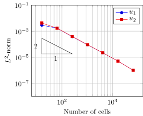
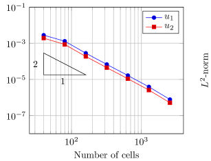
Figure 1. $L^{2}$ norm of the error in space with $\alpha_{1}=\alpha_{2}=1$ (left) and $\alpha_{1}=1$ and $\alpha_{2}=10$ (right); $p$ is defined in (42).

Next, we consider a two-dimensional test case on $\Omega=(0,1)\times(0,1)$ with $\Gamma^{D}=\{y=1\}$, $\Gamma^{N}=\partial\Omega\setminus\Gamma^{D}$, $u^{D}_{1}=u^{D}_{2}=0.1$, $\alpha_{1}=1$, $\alpha_{2}=5$, and the initial data

$$u^{0}_{1}(x,y)=u^{D}_{1}+u^{D}_{1}\,\mathbf{1}_{[0.2,0.5]}(x)\mathbf{1}_{[0,0.4]}(y),\quad u^{0}_{2}(x,y)=u^{D}_{2}+u^{D}_{2}\,\mathbf{1}_{[0.5,0.8]}(x)\mathbf{1}_{[0,0.4]}(y).$$

The mesh of $\Omega=(0,1)\times(0,1)$ is composed of 3584 triangles. In Figure 2, we show the evolution of the biomass $M$ at different times. It is shown in [13, Theorem 2.2] that the steady state is given by $u^{\infty}_{1}=u^{D}_{1}$ and $u^{\infty}_{2}=u^{D}_{2}$ and that the rate of convergence in the $L^{2}$ norm is of order $1/t$. Figure 2 (bottom right) shows this convergence to the steady state in the $L^{2}$ norm in a semi-logarithmic scale. We remark that the test case used here is close to that one used in [13]. The main difference is the absence of the source term in our case. It is worth mentioning that in this case, the rate of convergence of order $1/t$ seems to be sharp, while in [13], the authors observed an exponential convergence rate when the source term is given by $u^{D}_{i}-u_{i}$ for $i=1,\ldots,n$.

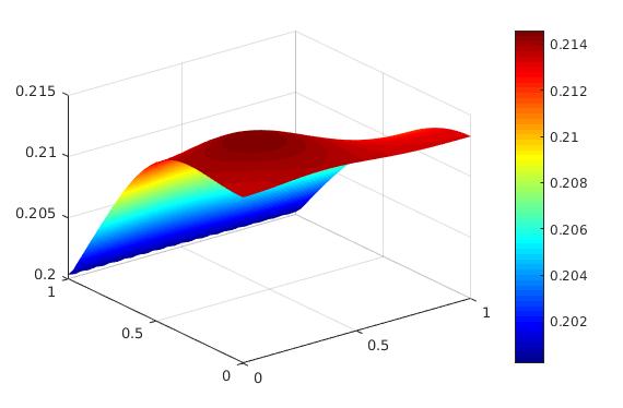
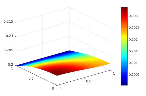
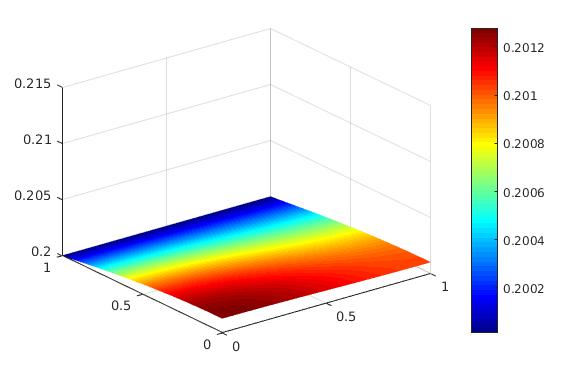
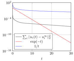
Figure 2. Evolution of the biomass $M$ at different times with $p$ defined in (42). Top left: $t=1$, top right: $t=5$, bottom left: $t=10$. Bottom right: Convergence of the solutions to the steady states in the $L^{2}$ norm with $p$ defined in (42).

7.3. Test case 2

We use a function $p$ that does not satisfy hypothesis (H4):

(43) $$p(x)=1-x\quad\mbox{for all }x\in[0,1]$$

and take $a=b=1$. Also here, we can also compute explicitly $q(M)/p(M)$:

$$\frac{q(M)}{p(M)}=\frac{M}{2(1-M)^{2}}.$$

As before, we consider first a one-dimensional test case on $\Omega=(0,1)$ with $\Gamma^{D}=\{0\}$, $\Gamma^{N}=\{1\}$, $u^{D}_{1}=u^{D}_{2}=0.1$, and the initial data

$$u^{0}_{1}(x)=u^{D}_{1}+u^{D}_{1}\mathbf{1}_{[0.2,0.5]}(x),\quad u^{0}_{2}(x)=u^{D}_{2}+u^{D}_{2}\mathbf{1}_{[0.5,0.8]}(x).$$

We investigate the $L^{2}$-convergence rate in space of the scheme for different values of $\alpha_{1}$ and $\alpha_{2}$; see Figure 3. We use the same strategy as described in the previous section. In particular, the scheme converges with an order around two.

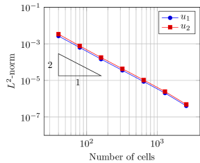
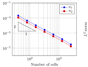
Figure 3. $L^{2}$ norm of the error in space with $\alpha_{1}=\alpha_{2}=1$ (left) and $\alpha_{1}=1$ and $\alpha_{2}=10$ (right); $p$ is defined in (43).

Finally, we consider a two-dimensional test case on $\Omega=(0,1)\times(0,1)$ with $\Gamma^{D}=\{y=1\}$, $\Gamma^{N}=\partial\Omega\setminus\Gamma^{D}$, $u^{D}_{1}=u^{D}_{2}=0.1$, $\alpha_{1}=1$, $\alpha_{2}=5$, and the initial data

$$u^{0}_{1}(x,y)=u^{D}_{1}+u^{D}_{1}\mathbf{1}_{[0.2,0.5]}(x)\mathbf{1}_{[0,0.4]}(y),\quad u^{0}_{2}(x,y)=u^{D}_{2}+u^{D}_{2}\mathbf{1}_{[0.5,0.8]}(x)\mathbf{1}_{[0,0.4]}(y).$$

Again, we choose a mesh of $\Omega=(0,1)\times(0,1)$ consisting of 3584 triangles. In Figure 4, we show the evolution of the biomass $M$ at different times and investigate the rate of convergence of the solution to the steady state $u^{\infty}_{1}=u^{D}_{1}$ and $u^{\infty}_{2}=u^{D}_{2}$. We represent the (squared) $L^{2}$ norm of the difference between $u_{i}$ and $u^{\infty}_{i}$ in a semi-logarithmic scale with final time $T=30$. Surprisingly, the rate of convergence seems to be better that the one of order $1/t$ obtained in [13, Theorem 2.2].

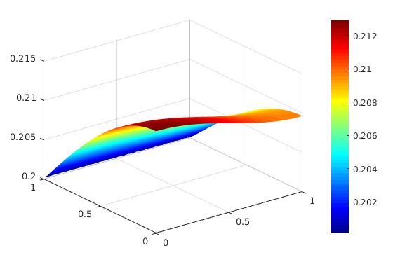
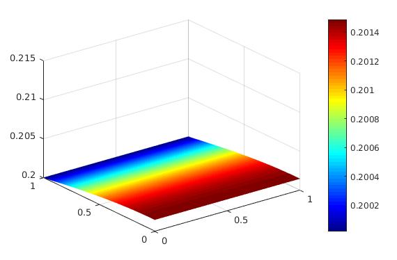
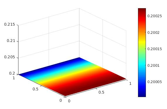
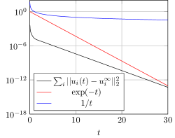
Figure 4. Evolution of the biomass $M$ at different times with $p$ defined in (43). Top left: $t=1$, top right: $t=5$, bottom: $t=10$. Bottom right: Convergence of the solutions to the steady states in $L^{2}$ norm with $p$ defined by (43).

References

- [1] A. Ait Hammou Oulhaj. Numerical analysis of a finite volume scheme for a seawater intrusion model with cross-diffusion in an unconfined aquifer. Numer. Meth. Partial Diff. Eqs. 34 (2018), 857–880.
- [2] V. Anaya, M. Bendahmane, M. Langlais, and M. Sepúlveda. A convergent finite volume method for a model of indirectly transmitted diseases with nonlocal cross-diffusion. Comput. Math. Appl. 70 (2015), 132–157.
- [3] V. Anaya, M. Bendahmane, and M. Sepúlveda. Numerical analysis for a three interacting species model with nonlocal and cross diffusion. ESAIM Math. Model. Numer. Anal. 49 (2015), 171–192.
- [4] B. Andreianov, M. Bendahmane, and R. R. Baier. Analysis of a finite volume method for a cross-diffusion model in population dynamics. Math. Models Meth. Appl. Sci. 21 (2011), 307–344.
- [5] B. Andreianov, C. Cancès, and A. Moussa. A nonlinear time compactness result and applications to discretization of degenerate parabolic-elliptic PDEs. J. Funct. Anal. 273 (2017), 3633–3670.
- [6] M. Bessemoulin-Chatard, C. Chainais-Hillairet, and F. Filbet. On discrete functional inequalities for some finite volume schemes. IMA J. Numer. Anal. 35 (2015), 1125–1149.
- [7] K. Brenner, C. Cancès and D. Hilhorst. Finite volume approximation for an immiscible two-phase flow in porous media with discontinuous capillary pressure. Comput. Geosci. 17 (2013), 573–597.
- [8] M. Burger, M. Di Francesco, J.-F. Pietschmann, and B. Schlake. Nonlinear cross-diffusion with size exclusion. SIAM J. Math. Anal. 42 (2010), 2842–2871.
- [9] C. Cancès, C. Chainais-Hillairet, A. Gerstenmayer, and A. Jüngel. Convergence of a finite-volume scheme for a degenerate cross-diffusion model for ion transport. Numer. Meth. Partial Diff. Eqs. 35 (2019), 545–575.
- [10] B. Capdeville and J. Rols. Introduction to biofilms in water and wastewater treatment. In: L. Melo, T. Bott, M. Fletcher, and B. Capdeville (eds.). Biofilms – Science and Technology. NATO ASI Series, vol. 223, pages 13–20. Springer, Dordrecht, 1992.
- [11] C. Chainais-Hillairet, J.-G. Liu, and Y.-J. Peng. Finite volume scheme for multi-dimensional drift-diffusion equations and convergence analysis. ESAIM: Math. Model. Numer. Anal. 37 (2003), 319–338.
- [12] K. Deimling. Nonlinear Functional Analysis. Springer, Berlin, 1985.
- [13] E. S. Daus, P. Milišić, and N. Zamponi. Analysis of a degenerate and singular volume-filling cross-diffusion system modeling biofilm growth. SIAM J. Math. Anal. 51 (2019), 3569–3605.
- [14] H. Eberl, D. Parker, and M. van Loosdrecht. A new deterministic spatio-temporal continuum model for biofilm development. J. Theor. Medicine 3 (2001), 161–175.
- [15] M. Efendiev, S. Zelik, and H. Eberl. Existence and longtime behavior of a biofilm model. Commun. Pure Appl. Anal. 8 (2009), 509–531.
- [16] R. Eymard, T. Gallouët, and R. Herbin. Finite volume methods. In: P. G. Ciarlet and J.-L. Lions (eds.), Handbook of Numerical Analysis 7 (2000), 713–1018.
- [17] A. Jüngel. The boundedness-by-entropy method for cross-diffusion systems. Nonlinearity 28 (2015), 1963–2001.
- [18] A. Jüngel and A. Zurek. A finite-volume scheme for a cross-diffusion model arising from interacting many-particle population systems. Submitted to Proceedings of the Conference “Finite Volumes in Complex Applications, Bergen, Norway, 2020. arXiv:1911.11426.
- [19] H. Murakawa. A linear finite volume method for nonlinear cross-diffusion systems. Numer. Math. 136 (2017), 1–26.
- [20] C. Nicolella, M. Van Loosdrecht, and J. Heijnen. Wastewater treatment with particulate biofilm reactors. J. Biotech. 80 (2000), 1–33.
- [21] K. Rahman and H. Eberl. Numerical treatment of a cross-diffusion model of biofilm exposure to antimicrobials. In: R. Wyrzykowski, J. Dongarra, K. Karczewski, and J. Waśniewski (eds.), Parallel Processing and Applied Mathematics. Part I, 134–144, Lect. Notes Comput. Sci. 8384, Springer, Heidelberg, 2014.
- [22] K. Rahman, R. Sudarsan, and H. Eberl. A mixed-culture biofilm model with cross-diffusion. Bull. Math. Biol. 77 (2015), 2086–2124.
- [23] S. Szego, P. Cinnella, and A. Cunningham. Numerical simulation of biofilm processes in closed circuits. J. Comput. Phys. 108 (1993), 246–263.
- [24] T. Yamamoto and S. Ueda. Numerical simulation of biofilm growth in flow channels using a cellular automaton approach coupled with a macro flow computation. Biorheology 50 (2013), 203–216.