Bilevel Optimization for Differentially Private Optimization in Energy Systems

Abstract

This paper studies how to apply differential privacy to constrained optimization problems whose inputs are sensitive. This task raises significant challenges since random perturbations of the input data often render the constrained optimization problem infeasible or change significantly the nature of its optimal solutions. To address this difficulty, this paper proposes a bilevel optimization model that can be used as a post-processing step: It redistributes the noise introduced by a differentially private mechanism optimally while restoring feasibility and near-optimality. The paper shows that, under a natural assumption, this bilevel model can be solved efficiently for real-life large-scale nonlinear nonconvex optimization problems with sensitive customer data. The experimental results demonstrate the accuracy of the privacy-preserving mechanism and showcases significant benefits compared to standard approaches.

I Introduction

Differential Privacy (DP) [1] is a robust framework used to measure and bound the privacy risks in computations over datasets: It has been successfully applied to numerous applications including histogram queries [2], census surveys [3, 4], linear regression [5] and deep learning [6] to name but a few examples. In general, DP mechanisms ensure privacy by introducing calibrated noise to the outputs or the objective of computations. However, its applications to large-scale, complex constrained optimization problems have been sparse.

This paper considers parametric optimization problems of the form

$${\cal O}(d)=\min_{x}f(x)\mbox{ s.t. }g(x,d)\geq 0,x\geq 0,$$ (OPT)

where $x$ is a vector of decision variables, $d$ is a real valued vector of problem inputs, and $g(x,d)$ is an abstract function capturing all the constraints on $x$ and $d$. Without loss of generality, the paper assumes that $x$ is non-negative. Given a vector $d^{o}$ of sensitive data, the task is to find a differentially private vector $d^{*}$ such that $d^{*}\approx d^{o}$ and ${\cal O}(d^{*})\approx{\cal O}(d^{o})$. Effective solutions to this task are useful in various settings, including the generation of differentially private test cases for (OPT) or in sequential coordination problems, e.g. sequential markets, in which agents need to exchange private versions of their data to solve ${\cal O}$. It is possible to use traditional differential privacy techniques (e.g., the ubiquitous Laplace or the Exponential mechanisms) to obtain a private vector $\tilde{d}$ such that $\tilde{d}\approx d^{o}$. However, in general, the optimization problem (OPT) may not admit any feasible solution for input $\tilde{d}$ or, its objective value ${\cal O}(\tilde{d})$ can be far from ${\cal O}(d^{o})$.

This paper aims at remedying this fundamental limitation. Given private versions $\tilde{d}$ of $d^{o}$ and $\tilde{f}$ of ${\cal O}(d^{o})$, it proposes a bilevel optimization model that leverages the post-processing immunity of differential privacy to produce a new private vector $d^{*}$, based on $\tilde{d}$, such that ${\cal O}(d^{*})\approx{\cal O}(d^{o})$. The paper also presents an algorithm that solves the bilevel model optimally under a natural monotonicity assumption. The effectiveness of the approach is demonstrated on large-scale case studies in electrical and gas networks where customer demands are sensitive, including nonlinear nonconvex benchmarks with more than $10^{4}$ variables. The paper generalizes prior approaches (e.g. [7]) designed to release benchmarks in energy systems. Its main contributions are as follows:

1. It presents a general mathematical framework, that relies on bilevel optimization, to obfuscate data $d^{o}$ of parametric optimization problems;

2. It proposes an efficient algorithm that solves the bilevel optimization model under a natural monotonicity assumption;

3. It demonstrates the effectiveness of the proposed method on two case studies on energy systems and empirically validates the monotonicity assumption on these case studies.

4. Finally, it demonstrates that optimal solutions to the bilevel model can produce significant improvements in accuracy compared to its relaxations.

II Related Work

The literature on theoretical results of Differential Privacy (DP) is huge (e.g., [8, 9]). The literature on DP applied to energy systems includes considerably fewer efforts. Ács and Castelluccia [10] exploit a direct application of the Laplace mechanism to hide user participation in smart meter datasets, achieving $\epsilon$-DP. Zhao et al. [11] study a DP schema that exploits the ability of households to charge and discharge a battery to hide the real energy consumption of their appliances. Liao et al. [12] introduce Di-PriDA, a privacy-preserving mechanism for appliance-level peak-time load balancing control in the smart grid, aimed at masking the consumption of top-k appliances of a household. Halder et al. [13] propose an architecture for privacy-preserving thermal inertial load management as a service provided by load-serving entities. Zhou et al. [14] later also present a particularly interesting relaxed notion of a (stronger) monotonicity property for a DC-OPF operator and shows how to use it to compute the operator sensitivity. This enables a characterization of the network sensitivity, which is useful to preserve the privacy of monotonic networks. A different line of work, conducted by Karapetyan et al. [15] quantifies empirically the trade-off between privacy and utility in demand response systems. The authors analyze the effects of a simple Laplace mechanism on the objective value of the demand response optimization problem. A DP schema that uses constrained post-processing was recently introduced by Fioretto et al. [16] and adopted to release private mobility data.

There are also related work on privacy-preserving implementations for the Alternating Direction Method of Multipliers (ADMM) algorithm. Zhang et al. [17] proposed a version of the ADMM algorithm for privacy-preserving empirical risk minimization problems, a class of convex problems used for regression and classification tasks. Huang et al. [18] proposed an approach that combines an approximate augmented Lagrangian function with time-varying Gaussian noise for general objective functions. Ding et al. [19] proposed P-ADMM, to provide guarantees within a relaxed model of differential privacy (called zero-concentrated DP). Finally, our recent work [20] proposed an ADMM formulation to obfuscate power system data for the data releasing process.

In contrast to previous work, this paper proposes a general solution for the releasing differentially private inputs of constrained optimization problems while guaranteeing solution feasibility and bounded distance to optimality. This work generalizes previous results [7] that apply to power systems. In addition, the paper extracts and reformulates the monotonicity property and provide proofs on the optimality of the algorithm under the monotonicity assumption. Experimental results on power and gas networks are also provided as empirical evidence for the monotonicity assumption.

TABLE I: Nomenclature.

$d\in{\cal N}$	Data vector $d$ from collection ${\cal N}$	$\alpha$	Indistinguishability parameter
$\epsilon$	Privacy parameter	$f$	Cost/Objective value
$\beta$	Cost acceptance threshold	${\cal S}$	Set of optimal solutions
${\cal F}$	Set of feasible solution	${\cal O}$	Parametric optimization problem (OPT)
$v^{o}/\tilde{v}$	The original / obfuscated value $v$	$v^{*}$	Optimally obfuscated value $v$

III Preliminaries

The traditional definition of differential privacy [1] aims at protecting the potential participation of an individual in a computation. For optimization problems however, the participants are typically known and the input is a vector $d=\langle d_{1},\ldots,d_{m}\rangle$, where $d_{i}$ represents a sensitive quantity associated with participant $i$. For instance, $d_{i}$ may represent the energy consumption of an industrial customer in an electrical transmission system. This privacy notion is best captured by the $\alpha$-indistinguishability framework proposed by Chatzikokolakis et al. [21] which protects the sensitive data of each individual up to some measurable quantity $\alpha>0$. As a result, this paper uses an adjacency relation $\sim_{\alpha}$ for input vectors defined as follows:

$$d\sim_{\alpha}d^{\prime}\Leftrightarrow\exists i\textrm{~{}s.t.~{}}|d_{i}-{d^{\prime}}_{i}|\leq\alpha\;\land\;d_{j}={d^{\prime}}_{j},\forall j\neq i,$$

where $d$ and ${d^{\prime}}$ are input vectors to (OPT) and $\alpha>0$ is a positive real value. This adjacency relation is used to protect an individual value $d_{i}$ up to privacy level $\alpha$ even if an attacker acquires information about all other inputs $d_{j}$ ($j\neq i$).

 Definition​ 1 (Differential Privacy).

Let $\alpha\!>\!0$. A randomized mechanism $\mathcal{M}\!:\!\mathcal{D}\!\to\!\mathcal{R}$ with domain $\mathcal{D}$ and range $\mathcal{R}$ is ($\epsilon,\alpha$)-indistinguishable if, for any output response $O\subseteq\mathcal{R}$ and any two adjacent input vectors $d$ and $d^{\prime}$ such that $d\sim_{\alpha}d^{\prime}$,

$$Pr[\mathcal{M}(d)\in O]\leq e^{\epsilon}Pr[\mathcal{M}({d^{\prime}})\in O].$$

Parameter $\epsilon\!\geq\!0$ controls the level of privacy, with small values denoting strong privacy, while $\alpha$ controls the level of indistinguishability. For notational simplicity, this paper assumes that $\epsilon$ is fixed to a constant and refers to mechanisms satisfying the definition above as $\alpha$-indistinguishable.

The post-processing immunity of DP [8] guarantees that a private dataset remains private even when subjected to arbitrary subsequent computations.

 Theorem​ 1 (Post-Processing Immunity).

Let $\mathcal{M}$ be an $\alpha$-indistinguishable mechanism and $g$ be a data-independent mapping from the set of possible output sequences to an arbitrary set. Then, $g\circ\mathcal{M}$ is $\alpha$-indistinguishable.

A real function $f$ over a vector $d$ can be made indistinguishable by injecting carefully calibrated noise to its output. The amount of noise to inject depends on the sensitivity $\Delta_{f}$ of $f$ defined as $\Delta_{f}=\max_{d\sim_{\alpha}{d^{\prime}}}\left\|f(d)-f({d^{\prime}})\right\|_{1}.$ For instance, querying a customer load from a dataset $d$ corresponds to an identity query whose sensitivity is $\alpha$. The Laplace mechanism achieves $\alpha$-indistinguishability by returning the randomized output $f(d)+z$, where $z$ is drawn from the Laplace distribution $\textrm{{\text{Lap}}}\left({\Delta_{f}}/{\epsilon}\right)$ [21].

Table I summarizes the notation adopted throughout the paper.

IV Differentially Private Optimization

IV-A Problem Definition

Consider the parametric optimization problem (OPT), a sensitive vector $d^{o}$, an $\alpha$-indistinguishable version $\tilde{d}$ of $d^{o}$, and an approximation $\tilde{f}$ of $f^{o}={\cal O}(d^{o})$. For instance, $\tilde{d}$ can be obtained by applying the Laplace mechanism on identity queries on all $d_{i}$; $\tilde{f}$ can be a private version of ${\cal O}(d^{o})$, or the value ${\cal O}(d^{o})$ itself if it is public which is typically the case when the optimization is a market-clearing mechanism, or an approximation of ${\cal O}(d^{o})$ obtained using public information only (e.g., a public forecast of $d^{o}$). The paper simply assumes that $|{\cal O}(d^{o})-\tilde{f}|\leq\beta^{o}$ for some user defined value $\beta^{o}>0$, which is not restrictive. Note that the assumption obviously holds when $f^{o}$ is public. The goal is to find a vector $d^{*}$ using only $\tilde{d}$, $\tilde{f}$, and the definition of (OPT) such that

$$d^{*}\approx\tilde{d}\mbox{ and }{\cal O}(d^{*})\approx\tilde{f}.$$

Observe that, by Theorem 1, $d^{*}$ will be $\alpha$-indistinguishable. It will be close to $d^{o}$ if $\tilde{d}$ is close to $d^{o}$. Moreover, (OPT) is feasible for $d^{*}$ and ${\cal O}(d^{*})$ will be close to ${\cal O}(d^{o})$ if $\tilde{f}$ is. The paper uses ${\cal S}(d)$ to denote the set of optimal solutions to (OPT), i.e.,

$${\cal S}(d)=\operatorname*{argmin}_{x}f(x)\mbox{ s.t. }g(x,d)\geq 0,x\geq 0,$$

and ${\cal F}(d)$ to denote the set of feasible solutions, i.e.,

$${\cal F}(d)=\{x\mid g(x,d)\geq 0,x\geq 0\}.$$

The paper assumes that ${\cal F}(d^{o})$ is not empty.

IV-B The Bilevel Optimization Model

The problem defined in Section IV-A can be tackled by a bilevel optimization model 1, i.e.,

$$d^{*}=\operatorname*{argmin}_{d} \;\;\|d-\tilde{d}\|^{2}_{2}$$ (BL1)

s.t. $$|{\cal O}(d)-\tilde{f}|\leq\beta.$$ (BL2)

Its output is a private $d^{*}$ whose L²-distance to $\tilde{d}$ is minimized and whose value ${\cal O}(d^{*})$ is in the interval $[\tilde{f}-\beta,\tilde{f}+\beta]$ for a parameter $\beta\geq\beta^{o}$. To make the bilevel nature more explicit, the above can be reformulated as

$$\min_{d,x^{*}} \;\;\|d-\tilde{d}\|^{2}_{2}$$ (BL1’)

s.t. $$|f(x^{*})-\tilde{f}|\leq\beta$$ (BL2’)

$$x^{*}=\operatorname*{argmin}_{x\geq 0}f(x)\mbox{ s.t. }g(x,d)\geq 0.$$ (Follower)

Note that $d^{o}$ is a feasible solution to (1), but not necessarily optimal. The set of optimal solutions to (1) is denoted by ${\cal S}^{BL}$ and the set of feasible solutions by ${\cal F}^{BL}$. If the private data $\tilde{d}$ satisfies (BL2) and does not require any post-processing, it is returned by model 1 (i.e. $d^{*}=\tilde{d}$).

 Theorem​ 2.

$d^{*}\in{\cal S}^{\it{BL}}$ implies $\|d^{*}-d^{o}\|_{2}\leq 2\|\tilde{d}-d^{o}\|_{2}.$

Proof.

Theorem 2 generalizes a prior result from [23, 7].

$$\|d^{*}-d^{o}\|_{2} \leq\|d^{*}-\tilde{d}\|_{2}+\|\tilde{d}-d^{o}\|_{2}$$

$$\leq 2\|\tilde{d}-d^{o}\|_{2}.$$

where the first inequality follows from the triangle inequality on norms and the second inequality follows from $\|d^{*}-d^{o}\|_{2}\leq\|d^{o}-\tilde{d}\|_{2}$ by optimality of $d^{*}$ and $d^{o}\in{\cal F}^{BL}$. ∎

It implies that, when a Laplace mechanism produces $\tilde{d}$, a solution $d^{*}\in{\cal S}^{\it{BL}}$ is no more than a factor of 2 away from optimality since the Laplace mechanism is optimal for identity queries [24]. In other words, (1) restores feasibility and near-optimality at a constant cost in accuracy. In practice, as shown in Section VI, $d^{*}$ is typically closer to $d^{o}$ than $\tilde{d}$ is.

IV-C High Point Relaxation (HPR)

Bilevel optimization is computationally challenging. It is strongly NP-hard [25] and even determining the optimality of a solution [26] is NP-hard. The High Point Relaxation (2), defined as

$$d^{h}=\operatorname*{argmin}_{d,x\geq 0} \;\;\|d-\tilde{d}\|^{2}_{2}$$ (HPR1)

s.t. $$g(x,d)\geq 0$$ (HPR2)

$$|f(x)-\tilde{f}|\leq\beta$$ (HPR3)

is an important tool in bilevel optimization. Due to the nature of relaxation, ${\cal O}(d^{h})\!\leq\!{\cal O}(d^{*})$. Theorem 2 also holds for (2), i.e., $\|d^{h}-d^{o}\|_{2}\!\leq\!2\|\tilde{d}-d^{o}\|_{2}$. The set of optimal solutions to (2) is denoted by ${\cal S}^{\it{HPR}}$ and its set of feasible solutions by ${\cal F}^{\it{HPR}}$. For simplicity, $(d,x)\in{\cal S}^{\it{P}}$ and $d\in{\cal S}^{\it{P}}$ are both used to denote an optimal solution to a problem (P) and its projection to $d$.

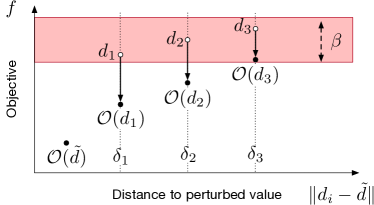
Figure 1: Illustrating the Intuition Underlying ${\cal O}^{\uparrow}$.

IV-D Solving the Bilevel Model

While bilevel optimization is, in general, computationally challenging, Model 1 presents a substantial structure: (Follower) minimizes $f$ but (BL2’) restrains it to be in a tight interval and (BL1’) keeps the potential solution close to $\tilde{d}$. The proposed solution technique leverages these observations and an additional insight derived from practical applications.

Intuition

Consider a pair $(\bar{d},\bar{x})$ such that $\bar{x}\geq 0$, $g(\bar{x},\bar{d})\geq 0$, and $|f(\bar{x})-\tilde{f}|\leq\beta$. Note that $\bar{x}$ is not necessarily an optimal solution (i.e., a minimizer) to Problem (Follower). However, if the optimal objective value ${\cal O}(\bar{d})$ is such that ${\cal O}(\bar{d})\geq\tilde{f}-\beta$, then $\bar{d}\in{\cal F}^{BL}$. The interesting case is when ${\cal O}(\bar{d})<\tilde{f}-\beta$. The proposed solution method recognizes that, in many optimization problems with sensitive data, $\bar{d}_{i}$ represents some data about participant $i$, such as her electricity consumption. Assume, for instance, that $\bar{d}$ represents the customer demands (the reasoning is similar if the data represents prices and reversed if the data represents production capabilities). By increasing $\bar{d}_{i}$, the value ${\cal O}(\bar{d})$ is expected to rise as well. The solution technique exploits this insight: It tries to find solutions that maximize the customer demands while staying within a small distance of $\tilde{d}$. In so doing, it restricts attention to input vectors in the set ${\cal N}$ defined as

$${\cal N}=\{d\mid\exists x\geq 0:g(x,d)\geq 0\mbox{ and }|f(x)-\tilde{f}\|\leq\beta\}.$$

Solution Method

This section presents an effective algorithm for solving the bilevel optimization problem (1) when (OPT) is monotone with respect to the sensitive data, capturing the above intuition.

 Definition​ 2 (Monotonicity).

(OPT) is monotone if there exists a proxy concave function $m:\Re^{m}\rightarrow\Re$ such that if, for all $d^{1},d^{2}\in{\cal N}$, $m(d^{1})\geq m(d^{2})\Rightarrow{\cal O}(d^{1})\geq{\cal O}(d^{2}).$

Note that the monotonicity assumption applies only to input vectors in ${\cal N}$. While monotonicity is unlikely to be true for general parametric optimization problems ${\cal O}$, since they can be nonconvex, the computational results reported in Section VI illustrates that this property holds on several real and realistic benchmarks.

To solve bilevel optimization problems over a monotone follower, the approach relies on solving optimization problems of the form

$${\cal O}^{\uparrow}(\delta)=\;\; \max_{d,x\geq 0}\hskip 24.18501pt\;\;m(d)$$ (PP1)

$$\text{subject to }\;\;g(x,d)\geq 0$$ (PP2)

$$\hskip 39.83368pt\;\;|f(x)-\tilde{f}|\leq\beta$$ (PP3)

$$\hskip 39.83368pt\;\;\|d-\tilde{d}\|^{2}_{2}\leq\ \delta$$ (PP4)

The set of optimal and feasible solutions to ${\cal O}^{\uparrow}(\delta)$ are denoted by ${\cal S}^{\uparrow}(\delta)$ and ${\cal F}^{\uparrow}(\delta)$ respectively. For a given $\delta$, ${\cal O}^{\uparrow}(\delta)$ finds a vector $\bar{d}\in{\cal N}$ that maximizes $m(\cdot)$ but remains within a distance $\delta$ of $\tilde{d}$ . Since, by monotonicity, $m(\cdot)$ is a proxy for maximizing the optimal cost for the optimization problem ${\cal O}(\cdot)$, the optimization can be viewed as searching for a feasible solution of (1) within a distance $\delta$ of $\tilde{d}$ which maximizes ${\cal O}(\cdot)$. Figure 1 illustrates the role of ${\cal O}^{\uparrow}$. Vector $d_{i}\in{\cal N}$ is the optimal solution of ${\cal O}^{\uparrow}(\delta_{i})$. As the distance $\delta_{i}$ increases, $d_{i}={\cal O}^{\uparrow}(\delta_{i})$ and ${\cal O}(d_{i})$ should increase as well.

Under the monotonicity assumption, (1) will be shown equivalent to the following optimization problem:

$$\min_{d,\delta\geq 0}\delta\mbox{ s.t. }[d\in S^{\uparrow}(\delta)\ \land\ {\cal O}(d)\geq\tilde{f}-\beta]$$ (BLM)

which is defined only in terms of ${\cal O}$ and ${\cal O}^{\uparrow}$. Observe that $\delta$ is a scalar and hence it is natural to solve (BLM) using binary search as depicted in Algorithm (1). The algorithm receives as input a tuple $\langle\delta^{l},\delta^{u},\eta\rangle$, where $\delta^{l}$ and $\delta^{u}$ are lower and upper bounds on the optimal value $\delta^{*}$ for (BLM), and produces an $\eta$-approximation to (BLM). Algorithm (1) is a simple binary search on the value $\delta$ alternating the optimizations of ${\cal O}$ and ${\cal O}^{\uparrow}$. For a given $\delta$, line 3 solves ${\cal O}^{\uparrow}$. If the resulting optimization satisfies the second constraint of (BLM), a new feasible solution to (1) is obtained and the upper bound can be updated. Otherwise, Algorithm (1) has identified a new lower bound. Note that, in practice, good lower and upper bounds are often available. For instance, it is possible to use an optimal solution $d^{h}$ of (2) and set $\delta^{l}=\delta^{h}=\|d^{h}-\tilde{d}\|^{2}_{2}$. To obtain $\delta^{u}$, one can start with $\delta^{h}$ and continue by doubling its value iteratively until Lemma 1 below applies.

1

Inputs : $\langle\delta^{l},\delta^{u},\eta\rangle$

Output : An $\eta$-approximation to (1)

2 while $\delta^{u}-\delta^{l}>\eta$ do

3       $\delta\leftarrow\frac{\delta^{l}+\delta^{u}}{2}$

4       solve ${\cal O}^{\uparrow}(\delta)$ and let $(d^{\uparrow},x^{\uparrow})$ be an optimal solution

5       $\delta^{\uparrow}\leftarrow\|d^{\uparrow}-\tilde{d}\|$

6       if ${\cal O}(d^{\uparrow})>\tilde{f}-\beta$ then  $\delta^{u}\leftarrow\delta^{\uparrow}\mbox{ {\bf else} }$ $\delta^{l}\leftarrow\delta$ ;

7      

return ${\cal S}^{\uparrow}(\delta^{u})$

Algorithm 1 Solving the BLM Optimization Problem.​​​​​

Correctness

It remains to prove the correctness of the solution technique. The following two lemmas capture important properties of ${\cal O}^{\uparrow}$. The first lemma shows that, when $\delta$ is large enough, ${\cal O}^{\uparrow}(\delta)$ always returns a feasible solution to (1).

 Lemma​ 1.

Let $\delta^{o}=\|d^{o}-\tilde{d}\|_{2}^{2}\leq\delta^{o}$ and $(d^{\uparrow},x^{\uparrow})\in{\cal S}^{\uparrow}(\delta^{o})$. Then $d^{\uparrow}\in{\cal F}^{BL}$.

Proof.

By definition of $\delta^{o}$, $d^{o}\in{\cal F}^{\uparrow}(\delta^{o})$ and there exists $x^{o}$ such that the pair $(d^{o},x^{o})$ satisfies conditions (PP2)–(PP4). Since $(d^{\uparrow},x^{\uparrow})\in{\cal S}^{\uparrow}(\delta^{o})$, $m(d^{\uparrow})\geq m(d^{o})$ and, by monotonicity, ${\cal O}(d^{\uparrow})\geq{\cal O}(d^{o})\geq\tilde{f}-\beta$. By (PP3), $f(x^{\uparrow})\leq f^{o}+\beta$ and, by (PP2), ${\cal O}(d^{\uparrow})\leq f(x^{\uparrow})$. Hence

$$\tilde{f}+\beta\geq f(x^{\uparrow})\geq{\cal O}(d^{\uparrow})\geq{\cal O}(d^{o})\geq\tilde{f}-\beta$$

and $d^{\uparrow}$ satisfies (BL2). ∎

The second lemma shows that there is no feasible solution to (1) within distance $\dot{\delta}$ of $\tilde{d}$ when ${\cal O}(\dot{\delta})$ returns a solution $d$ that violates (BL2).

 Lemma​ 2.

Let $(\dot{d},\dot{x})\in{\cal S}^{\uparrow}(\dot{\delta})$ and ${\cal O}(\dot{d})<\tilde{f}-\beta$. Then,

$$\forall d^{f}\in{\cal F}^{BL}:\|d^{f}-\tilde{d}\|_{2}^{2}>\dot{\delta}.$$

Proof.

Consider $d^{f}\in{\cal F}^{BL}$ and assume that $\|d^{f}-\tilde{d}\|_{2}^{2}\leq\dot{\delta}$, which implies that $d^{f}\in{\cal F}^{\uparrow}(\dot{\delta})$. By optimality of $\dot{d}$, $m(\dot{d})\geq m(d^{f})$ and, by monotonicity, ${\cal O}(\dot{d})\geq{\cal O}(d^{f})$. By (BL2), ${\cal O}(d^{f})\geq\tilde{f}-\beta$ which contradicts ${\cal O}(\dot{d})<\tilde{f}-\beta$. ∎

These two lemmas make it possible to prove the equivalence of (1) and (BLM) when (OPT) is monotone.

 Theorem​ 3.

When (OPT) is monotone, (1) and (BLM) are equivalent.

Proof.

Let $(d^{*},\delta^{*})$ be the optimal solution to (BLM). Such a solution always exists by Lemma 1 and $\|d^{*}-\tilde{d}\|_{2}^{2}\leq\delta^{*}$. By definition of ${\cal O}^{\uparrow}$, ${\cal F}(d^{*})\neq\emptyset$ and ${\cal O}(d^{*})\leq\tilde{f}+\beta$. Since ${\cal O}(d^{*})\geq\tilde{f}-\beta$ by definition of (BLM), $d^{*}\in{\cal F}^{BL}$.

Consider now $\delta^{-}<\delta^{*}$ and a solution $d^{-}\in{\cal S}^{\uparrow}(\delta^{-})$. If such a solution exists, ${\cal O}(d^{-})<f^{o}-\beta$ by optimality of $\delta^{*}$. By Lemma 2, it comes that $\forall d^{f}\in{\cal F}^{BL}:\|d^{f}-\tilde{d}\|_{2}^{2}>\delta^{-}.$ Hence, $d^{*}$ is also optimal for (1). ∎

It remains to show that the algorithm computes an $\eta$-approximation.

 Theorem​ 4.

Algorithm (1) computes an $\eta$-approximation of (1) when (OPT) is monotone.

Proof.

Let $d^{*}$ be an optimal solution to (1). Upon termination of Algorithm (1), it comes that $\delta^{l}\leq\|d^{*}-\tilde{d}\|^{2}_{2}\leq\delta^{u}.$ Moreover, if $d^{u}\in S^{\uparrow}(\delta^{u})$, it follows that $\|d^{u}-\tilde{d}\|^{2}_{2}\leq\delta^{u}$. Hence, $\delta^{l}\leq\|d^{*}-\tilde{d}\|^{2}_{2}\leq\|d^{u}-\tilde{d}\|^{2}_{2}\leq\delta^{u}.$ ∎

Discussion

In general, bilevel optimization is extremely difficult and general techniques and reformulations are often challenging to solve. This paper isolates a class of bilevel problems where the optimal cost of the follower subproblem can be inferred, through monotonicity, by a proxy function that depends on variables controlling also the costs of the leader problem (BL1). In game-theoretical settings, the proxy function serves as a bridge between the leader decisions to the costs of the follower. The existence of such a monotone function $m$ depends on the privacy application but is natural in energy systems where the customer load/demand must be protected. Indeed, the load appears linearly in flow balance constraints and load increases almost always lead to cost increases. Exploring other classes of problems (e.g. bounded monotonicity) will be left as future work.

V Applications on Energy Systems

Model 1 ${\cal O}_{\text{OPF}}$: AC Optimal Power Flow

variables: $$S^{g}_{i},V_{i}\;\;\forall i\in N,\;\;S_{ij}\;\;\forall(i,j)\in E\cup E^{R}$$

minimize: $${\mathcal{O}}(\bm{S^{d}})=\sum_{i\in N}{c}_{2i}(\Re(S^{g}_{i}))^{2}+{c}_{1i}\Re(S^{g}_{i})+{c}_{0i}$$ (3)

subject to: $$\angle V_{i}=0,\;\;i=\min N$$ (4)

$${v}^{l}_{i}\leq|V_{i}|\leq{v}^{u}_{i}\;\;\forall i\in N$$ (5)

$${\theta}^{l}_{ij}\leq\angle(V_{i}V^{*}_{j})\leq{\theta}^{u}_{ij}\;\;\forall(i,j)\in E$$ (6)

$${S}^{gl}_{i}\leq S^{g}_{i}\leq{S}^{gu}_{i}\;\;\forall i\in N$$ (7)

$$|S_{ij}|\leq{s}^{u}_{ij}\;\;\forall(i,j)\in E\cup E^{R}$$ (8)

$$S^{g}_{i}-{S}^{d}_{i}=\textstyle\sum_{(i,j)\in E\cup E^{R}}S_{ij}\;\;\forall i\in N$$ (9)

$$S_{ij}={Y}^{*}_{ij}|V_{i}|^{2}-{Y}^{*}_{ij}V_{i}V^{*}_{j}\;\;\forall(i,j)\in E\cup E^{R}$$ (10)

This section describes two substantial case studies for evaluating the privacy mechanism: optimal power flow in electricity networks and optimal compressor optimization in gas networks. Both models are nonlinear and nonconvex.

Optimal Power Flow

Optimal Power Flow (OPF) is the problem of finding the best generator dispatch to meet the demands in a power network. A power network $\bm{\mathcal{N}}$ can be represented as a graph $(N,E)$, where the nodes in $N$ represent buses and the edges in $E$ represent lines. The edges in $E$ are directed and $E^{R}$ is used to denote those arcs in $E$ but in reverse direction. The AC power flow equations are based on complex quantities for current $I$, voltage $V$, admittance $Y$, and power $S$, and these equations are a core building block in many power system applications. Model 1 shows the AC OPF formulation, with variables/quantities shown in the complex domain. Superscripts $u$ and $l$ are used to indicate upper and lower bounds for variables. The objective function ${\mathcal{O}}(\bm{S^{g}})$ captures the cost of the generator dispatch, with $\bm{S^{g}}$ denoting the vector of generator dispatch values $(S^{g}_{i}\>|\>i\in N)$. Constraint (4) sets the reference voltage angle to zero for the slack bus $i\in N$ to eliminate numerical symmetries. Constraints (5) bound the voltage magnitudes, and constraints (6) limit the voltage angle differences for every transmission lines/transformers. Constraints (7) enforce the generator output limits, and constraints (8) impose the line flow limits. Finally, constraints (9) capture Kirchhoff’s Current Law imposing the flow balance across every node, and constraints (10) capture Ohm’s Law describing the AC power flow across lines/transformers.

Model 2 ${\cal O}_{\text{OGF}}$: Optimal Gas Flow

variables: $$p_{i},q_{i}\;\forall i\in\mathcal{J},\;q_{ij}\;\forall(i,j)\in\mathcal{P},\;R_{ij}\;\forall(i,j)\in\mathcal{C}$$

minimize: $${\mathcal{O}}(\bm{q})=\sum_{(i,j)\in C}\mu^{-1}|q_{ij}|(\max\{R_{ij},1\}^{2(\gamma-1)/\gamma}-1)$$ (11)

subject to: $$\textstyle\sum_{(i,j)\in\mathcal{P}}q_{ij}-\sum_{(j,i)\in\mathcal{P}}q_{ji}=q_{i},\;\;\forall i\in\mathcal{J}$$ (12)

$${p_{i}}^{l}\leq p_{i}\leq{p_{i}}^{u}\;\;\forall i\in N,\;\;{q_{ij}}^{l}\leq q_{ij}\leq{q_{ij}}^{u}\;\;\forall(i,j)\in\mathcal{P}$$ (13)

$${R_{ij}}^{l}\leq R_{ij}\leq{R_{ij}}^{u}\;\;\forall(i,j)\in\mathcal{C}$$ (14)

$$p_{i}=p^{T}_{i}\;\;\forall i\in\mathcal{J}^{B},q_{i}=0\;\;\forall i\in\mathcal{J}^{T},q_{i}=q^{d}_{i}\;\;i\in\mathcal{J}^{D}$$ (15)

$$R_{ij}^{2}p_{i}^{2}-p_{j}^{2}=L_{ij}\displaystyle\frac{\lambda a^{2}}{D_{ij}A_{ij}^{2}}q_{ij}\lvert q_{ij}\rvert\;\;\forall(i,j)\in\mathcal{C}$$ (16)

$$p_{i}^{2}-p_{j}^{2}=L_{ij}\displaystyle\frac{\lambda a^{2}}{D_{ij}A_{ij}^{2}}q_{ij}\lvert q_{ij}\rvert\;\;\forall(i,j)\in\mathcal{P}-\mathcal{C}$$ (17)

Optimal Compressor Optimization

Optimal Gas Flow (OGF) is the problem of finding the best compression control to maintain pressure requirements in a natural gas pipeline system. A natural gas network can be represented as a directed graph $\bm{\mathcal{N}}=(\mathcal{J},\mathcal{P})$, where a node $i\in\mathcal{J}$ represents a junction point and an edge $(i,j)\in\mathcal{P}$ represents a pipeline. Compressors ($\mathcal{C}\subseteq\mathcal{P}$) are installed in a subset of the pipelines for boosting the gas pressure $p$ in order to maintain pressure requirements for gas flow $q$. The set $\mathcal{J}^{D}$ of gas demands and the set $\mathcal{J}^{T}$ of transporting nodes are modeled as junction points, with net gas flow $q_{i}$ set to the gas demand ($q^{d}_{i}$) and zero respectively. For simplicity, the paper assumes no pressure regulation and losses within junction nodes and gas flow/flux are conserved throughout the system. A subset $\mathcal{J}^{B}\in\mathcal{J}$ of the nodes are regulated with constant pressure $p^{T}_{i}$. The length of pipe $(i,j)$ is denoted by $L_{ij}$, its diameter by $D_{ij}$, and its cross-sectional area by $A_{ij}$. Universal quantities include isentropic coefficient $\gamma$, compressor efficiency factor $\mu$, sound speed $a$, and gas friction factor $\lambda$. Model 2 depicts the OGF formulation. The objective function ${\mathcal{O}}(\bm{q})$ captures the compressor costs using the compressor control values $(R_{ij}\>|\>(i,j)\in\mathcal{C})$. Constraints (12) capture the flow conversation equations. Constraints (13) and (14) capture the pressure, flux flow, and compressor control bounds. Constraints (15) set the boundary conditions for the demands and the regulated pressures. Finally, constraints (16) and (17) capture the steady-state isothermal gas flow equation that describes the pressure loss mechanics within gas pipes.

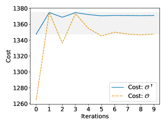
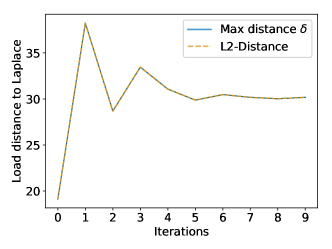
Figure 2: Gaslib-135: OGF costs and L²-distance to $\tilde{\delta}$ as a function of the number of iterations for parameters $\alpha=0.1$ and $\beta=1\%$.

Obfuscation

In both networks, customer demands are sensitive and are associated with customer activities. These quantities always appear in the flow conservation constraints, which are linear. Increasing these values obviously requires more (electricity and gas) production and hence one can expect the cost to increase. This is not always the case, because of the engineering constraints on voltages and pressures and the lower bounds of the production units, for instance. However, in practice, because of reliability constraints, these constraints are rarely binding at optimality and one may expect the systems to behave monotonically around the optimality point. The above is validated in the experimental results.

VI Experimental Evaluation

Setting

The experiments were performed on a variety of NESTA power systems [27] and natural gas test systems from [28], including test instances from GasLib [29]. Parameter $\epsilon$ is fixed to 1.0 and the indistinguishability level $\alpha$ varies from $10^{-1}$ to $10^{1}$ (in per unit notation). The fidelity parameter $\beta$ varies from 0.1% to 10% of value $\tilde{f}=f^{o}$. Convergence parameter $\eta$ is set to $10^{-3}$ (in per unit). The lower bounds and upper bounds are initialized as specified in prior sections. The solution technique is limited to 3000 calls to ${\cal O}^{\uparrow}$. The models are implemented with PowerModels.jl [30] with the nonlinear solver IPOPT [31]. Note that some of the test cases have more than $10^{4}$ variables.

Behavior of the Solution Technique

Figure 2 shows how the costs (${\cal O}$ and ${\cal O}^{\uparrow}$) and L²-Distance to $\tilde{\delta}$ typically change when running Algorithm 1 and its initialization. The L²-Distance to $\tilde{d}$ increases initially to find a solution within the feasible cost range (shaded area). The binary search then finds the optimal distance in a few iterations. (PP4) is usually binding when optimizing ${\cal O}^{\uparrow}$.

TABLE II: OPF: Average CPU times and number of optimizations (50 runs) for parameters $\alpha=\{0.1,1.0,10.0\}$ and $\beta=1\%$.

$\alpha$	$0.1$	$1.0$	$10.0$	$0.1$	$1.0$	$10.0$
Benchmark	Time (s)	Time (s)	Time (s)	Opt.	Opt.	Opt.
case14_ieee	0.71	0.58	1.01	10.22	4.40	6.10
case24_ieee_rts	1.52	1.40	2.30	8.90	4.14	5.10
case29_edin	0.67	36.84	23.50	1.00	40.36	27.78
case30_as	0.90	0.90	0.85	4.62	4.28	3.80
case30_fsr	1.28	1.07	0.66	6.24	4.70	2.82
case30_ieee	0.84	1.22	1.33	5.14	5.86	6.06
case39_epri	1.16	6.92	1.29	6.32	21.50	3.14
case57_ieee	1.77	4.22	10.31	4.98	3.72	7.94
case73_ieee_rts	6.20	2.17	11.571	9.88	1.62	66.54
case89_pegase	9.23	13.56	17.60	6.04	5.26	7.82
case118_ieee	10.15	10.71	9.77	10.08	5.96	6.42
case162_ieee_dtc	10.04	35.18	53.72	4.88	9.68	8.82
case189_edin	2.98	53.40	58.08	2.16	7.98	8.18
case240_wecc	12.34	117.78	148.16	1.16	10.88	10.10
case300_ieee	1621.78	360.99	301.32	8.90	7.98	10.32
case1354_pegase	15.90	2172.23	2363.19	1.16	7.68	9.10
case1394sop_eir	70.78	777.66	1427.87	3.72	6.12	5.40
case1397sp_eir	146.47	1298.15	660.12	3.90	6.40	4.60
case1460wp_eir	157.06	1418.58	728.84	4.72	6.90	5.66

TABLE III: OGF: Average CPU times and number of optimizations (50 runs) for parameters $\alpha=\{0.1,1.0,2.0\}$ and $\beta=1\%$.

$\alpha$	$0.1$	$1.0$	$2.0$	$0.1$	$1.0$	$2.0$
Benchmark	Time (s)	Time (s)	Time (s)	Opt.	Opt.	Opt.
24-pipe	2.34	0.67	1.77	20.56	6.20	6.22
GasLib-40	34.74	141.16	132.65	26.50	33.48	28.82
GasLib-135	21.63	28.91	214.57	12.96	8.74	25.80

TABLE IV: OPF test cases: Average OPF cost difference (in %) for parameters $\alpha=0.1$ and $\beta=\{10\%,1\%,0.1\%\}$.

	Bi-level			High-point
$\beta(\%)$	$10\%$	$1\%$	$0.1\%$	$10\%$	$1\%$	$0.1\%$
case14_ieee	0.1	0.1	0.0	-4.9	-6.2	-6.3
case24_ieee_rts	0.0	0.4	0.1	-0.1	-1.6	-1.9
case29_edin	-0.0	-0.0	0.0	-0.0	-0.0	-0.1
case30_as	0.7	0.3	-0.1	-1.1	-2.3	-2.4
case30_fsr	-0.1	0.3	-0.1	-6.2	-6.8	-6.9
case30_ieee	-0.3	0.1	0.0	-2.7	-1.8	-1.6
case39_epri	-0.2	-0.0	0.0	-0.2	-0.4	-0.7
case57_ieee	1.5	0.4	0.1	1.4	-0.6	-1.0
case73_ieee_rts	-0.4	0.1	0.0	-0.4	-1.1	-1.4
case89_pegase	-0.3	-0.1	0.0	-0.3	-0.4	-0.6
case118_ieee	-0.0	0.3	0.0	-0.0	-1.6	-2.0
case162_ieee_dtc	2.6	0.5	0.1	2.3	-0.1	-0.7
case189_edin	9.2	1.0	0.1	9.2	0.8	-0.1
case240_wecc	0.4	0.1	0.0	0.4	0.1	-0.2
case300_ieee	8.9	0.9	0.1	8.8	0.9	0.1
case1354_pegase	0.0	0.0	0.0	0.0	0.0	-0.1
case1394sop_eir	9.8	1.0	0.1	10.3	1.2	0.3
case1397sp_eir	10.0	1.0	0.1	10.5	2.0	0.7
case1460wp_eir	9.8	1.0	0.1	14.6	1.5	0.7

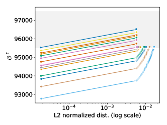
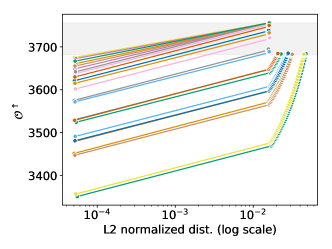
Figure 3: IEEE-39 (left) IEEE-118 (right): OPF cost as a function of the L²-distance to $\tilde{\delta}$ for parameters $\alpha=0.1$ and $\beta=1\%$.

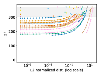
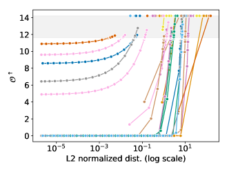
Figure 4: 24-pipe (left) Gaslib-40 (right): OGF cost as a function of the L²-distance to $\tilde{\delta}$ for parameters $\alpha=0.1$ and $\beta=10\%$.

Convergence and Computational Efficiency

The experimental results demonstrate the robustness and scalability of the approach. Tables II and III depict the average CPU times (in seconds) and average number of calls to ${\cal O}^{\uparrow}$ (and thus ${\cal O}$) also over 50 runs. All instances (except one) converge with a very small number of iterations. Even large-scale test cases with more than $10^{4}$ variables are solved in a few iterations. The bilevel model is thus a truly practical approach to demand obfuscation of these networks.

Monotonicity

Figures 3 and 4 illustrate the interpolation of the optimal values ${\cal O}^{\uparrow}$ (y-axis) with the respect to their distances to $\tilde{\delta}$ (x-axis) obtained while solving the bilevel model. The shaded area shows the feasible cost range. The results summarize 50 runs (each with a different random seed), each represented by a colored curve. As can be seen, the monotonicity property holds in these real networks. Note also the single points in the gas plot: These are cases where the high-point relaxation can be made optimal in one iteration.

The Benefits of the Bilevel Model

Tables IV and V show the benefits of the bilevel model compared to the HPR. The HPR returns a solution $d^{h}$ in ${\cal N}$ with the smallest distance to $\tilde{d}$. However, it is typically the case that ${\cal O}(d^{h})<\tilde{f}-\beta$. The tables report the relative distance of ${\cal O}(d^{*})$ and ${\cal O}(d^{h})$ to $\tilde{f}$ for various values of $\beta$. Numbers are bold for instances violating the $\beta$ thresholds. Table V shows that, on the gas networks, the bilevel model produces several orders of magnitude improvements over the HPR. The gains are less pronounced on the electricity systems, but remain substantial. Note that obfuscation methods with a few percents of cost difference mean an obfuscation error of hundreds of millions of dollars in energy systems.

TABLE V: OGF test cases: Average OGF cost differences (in %) for parameters $\alpha=0.1$ and $\beta=\{10\%,1\%,0.1\%\}$.

	Bi-level			High-point
$\beta(\%)$	$10\%$	$1\%$	$0.1\%$	$10\%$	$1\%$	$0.1\%$
24-pipe	-3.1	-0.3	0.0	-12.1	-13.7	-14.1
gaslib-40	2.5	0.3	0.0	-31.5	-38.1	-39.0
gaslib-135	1.3	0.2	0.0	-37.3	-38.4	-41.6

TABLE VI: OPF test cases: Average distance (L2, normalized to original scale) between obfuscated and original solutions for parameters $\alpha=\{0.1,1.0,10.0\}$ and $\beta=1\%$.

	Bi-level			High-point			Laplace
$\alpha$ (p.u.)	$0.1$	$1.0$	$10.0$	$0.1$	$1.0$	$10.0$	$0.1$	$1.0$	$10.0$
case14_ieee	0.67	4.48	10.32	0.67	4.51	10.60	0.71	7.08	70.82
case24_ieee_rts	0.13	1.11	3.61	0.13	1.11	3.63	0.13	1.34	13.39
case29_edin	0.01	0.09	0.82	0.01	0.09	0.82	0.01	0.09	0.87
case30_as	0.84	3.34	4.45	0.84	3.35	4.49	0.97	9.74	97.43
case30_fsr	1.42	5.47	7.40	1.43	5.49	7.47	1.66	16.61	166.14
case30_ieee	0.88	3.86	5.46	0.88	3.88	5.60	0.97	9.74	97.43
case39_epri	0.06	0.60	2.44	0.06	0.60	2.44	0.06	0.62	6.24
case57_ieee	0.34	2.38	6.64	0.34	2.42	7.56	0.35	3.51	35.14
case73_ieee_rts	0.13	1.11	3.65	0.13	1.11	3.67	0.13	1.32	13.19
case89_pegase	0.06	0.53	2.64	0.06	0.53	2.86	0.06	0.56	5.60
case118_ieee	0.40	3.03	6.85	0.40	3.04	6.87	0.40	3.99	39.89
case162_ieee_dtc	0.09	0.68	1.59	0.10	0.69	1.61	0.10	0.96	9.62
case189_edin	0.34	2.05	3.92	0.34	2.07	4.18	0.35	3.50	35.05
case240_wecc	0.01	0.12	0.99	0.01	0.12	1.01	0.01	0.12	1.23
case300_ieee	0.10	0.85	3.69	0.10	0.86	4.46	0.11	1.07	10.65
case1354_pegase	0.14	1.26	5.47	0.14	1.26	6.21	0.14	1.36	13.59

TABLE VII: OGF test cases: Average distance (L2, normalized to original scale) between obfuscated and original solutions for parameters $\alpha=\{0.1,0.4,1.0\}$ and $\beta=1\%$.

	Bi-level			High-point			Laplace
$\alpha$ (p.u.)	$0.1$	$0.4$	$1.0$	$0.1$	$0.4$	$1.0$	$0.1$	$0.4$	$1.0$
24-pipe	0.32	1.24	2.68	0.34	1.29	2.71	0.36	1.43	3.58
gaslib-40	2.04	7.66	22.13	1.95	7.51	16.54	2.01	8.03	20.07
gaslib-135	0.72	2.78	7.30	0.72	2.75	6.46	0.72	2.88	7.19

Obfuscation Quality

Tables VI and VII report the L²-distances to the original loads for the high-point relaxation, the bilevel model, and the load vector $\tilde{d}$ (which typically produces infeasible problems). The results are averaged over 50 runs. The results show that the fidelity of the bilevel model (i.e., how close $d^{*}$ is to $d^{o}$) is extremely high, and often improves over the fidelity of the HPR. Finally, the bilevel model has a much higher fidelity than the Laplace mechanism.

VII Conclusion

This paper presented a bilevel optimization model for postprocessing the differentially private input of a constrained optimization problem. The model restores the feasibility and near-optimality of the optimization problem. The paper shows that the bilevel model can be solved effectively under a natural monotonicity assumption by alternating the solving of the follower problem and the solving of a novel optimization model that maximizes a proxy of the true objective. Experimental results on large-scale nonconvex constrained optimization problems with more than $10^{4}$ variables demonstrate the accuracy, efficiency, and benefits of the approach. They also validate the monotonicity assumptions empirically. Future work will be devoted to understanding and characterizing theoretically the solution space around optimal solutions.

References

- [1] C. Dwork, F. McSherry, K. Nissim, and A. Smith, “Calibrating noise to sensitivity in private data analysis,” in TCC, vol. 3876. Springer, 2006, pp. 265–284.
- [2] C. Li, M. Hay, V. Rastogi, G. Miklau, and A. McGregor, “Optimizing linear counting queries under differential privacy,” in Proceedings of the twenty-ninth ACM SIGMOD-SIGACT-SIGART symposium on Principles of database systems. ACM, 2010, pp. 123–134.
- [3] J. M. Abowd, “The us census bureau adopts differential privacy,” in Proceedings of the 24th ACM SIGKDD International Conference on Knowledge Discovery & Data Mining. ACM, 2018, pp. 2867–2867.
- [4] F. Fioretto and P. Van Hentenryck, “Differential privacy of hierarchical census data: An optimization approach,” in Principles and Practice of Constraint Programming - 25th International Conference, CP, 2019, pp. 639–655.
- [5] K. Chaudhuri, C. Monteleoni, and A. D. Sarwate, “Differentially private empirical risk minimization,” Journal of Machine Learning Research, vol. 12, no. Mar, pp. 1069–1109, 2011.
- [6] M. Abadi, A. Chu, I. Goodfellow, H. B. McMahan, I. Mironov, K. Talwar, and L. Zhang, “Deep learning with differential privacy,” in Proceedings of the 2016 ACM SIGSAC Conference on Computer and Communications Security. ACM, 2016, pp. 308–318.
- [7] T. Mak, F. Fioretto, L. Shi, and P. Van Hentenryck, “Privacy-preserving power system obfuscation: A bilevel optimization approach,” IEEE Transactions on Power Systems, vol. 35, no. 2, pp. 1627–1637, 2020.
- [8] C. Dwork and A. Roth, “The algorithmic foundations of differential privacy,” Theoretical Computer Science, vol. 9, no. 3-4, pp. 211–407, 2013.
- [9] S. Vadhan, “The complexity of differential privacy,” in Tutorials on the Foundations of Cryptography. Springer, 2017, pp. 347–450.
- [10] G. Ács and C. Castelluccia, “I have a dream!(differentially private smart metering).” in Information hiding, vol. 6958. Springer, 2011, pp. 118–132.
- [11] J. Zhao, T. Jung, Y. Wang, and X. Li, “Achieving differential privacy of data disclosure in the smart grid,” in INFOCOM, 2014 Proceedings IEEE. IEEE, 2014, pp. 504–512.
- [12] X. Liao, P. Srinivasan, D. Formby, and A. R. Beyah, “Di-prida: Differentially private distributed load balancing control for the smart grid,” IEEE Transactions on Dependable and Secure Computing, 2017.
- [13] A. Halder, X. Geng, P. R. Kumar, and L. Xie, “Architecture and algorithms for privacy preserving thermal inertial load management by a load serving entity,” IEEE Transactions on Power Systems, vol. 32, no. 4, pp. 3275–3286, July 2017.
- [14] F. Zhou, J. Anderson, and S. H. Low, “Differential privacy of aggregated dc optimal power flow data,” in 2019 American Control Conference (ACC), 2019, pp. 1307–1314.
- [15] A. Karapetyan, S. K. Azman, and Z. Aung, “Assessing the privacy cost in centralized event-based demand response for microgrids,” CoRR, vol. abs/1703.02382, 2017. [Online]. Available: http://arxiv.org/abs/1703.02382
- [16] F. Fioretto, C. Lee, and P. Van Hentenryck, “Constrained-based differential privacy for private mobility,” in Proceedings of the International Joint Conference on Autonomous Agents and Multiagent Systems (AAMAS), 2018, pp. 1405–1413.
- [17] T. Zhang and Q. Zhu, “Dynamic differential privacy for ADMM-based distributed classification learning,” IEEE Transactions on Information Forensics and Security, vol. 12, no. 1, pp. 172–187, 2016.
- [18] Z. Huang, R. Hu, Y. Guo, E. Chan-Tin, and Y. Gong, “DP-ADMM: ADMM-based distributed learning with differential privacy,” IEEE Transactions on Information Forensics and Security, 2019.
- [19] J. Ding, Y. Gong, M. Pan, and Z. Han, “Optimal differentially private ADMM for distributed machine learning,” arXiv preprint arXiv:1901.02094, 2019.
- [20] T. W. Mak, F. Fioretto, and P. Van Hentenryck, “Privacy-preserving obfuscation for distributed power systems,” Electric Power Systems Research, vol. 189, p. 106718, 2020.
- [21] K. Chatzikokolakis, M. E. Andrés, N. E. Bordenabe, and C. Palamidessi, “Broadening the scope of differential privacy using metrics,” in International Symposium on Privacy Enhancing Technologies Symposium. Springer, 2013, pp. 82–102.
- [22] C. Dwork, “A firm foundation for private data analysis,” Communications of the ACM, vol. 54, no. 1, pp. 86–95, 2011.
- [23] F. Fioretto and P. Van Hentenryck, “Constrained-based differential privacy: Releasing optimal power flow benchmarks privately,” in Proceedings of Integration of Constraint Programming, Artificial Intelligence, and Operations Research (CPAIOR), 2018, pp. 215–231.
- [24] F. Koufogiannis, S. Han, and G. J. Pappas, “Optimality of the laplace mechanism in differential privacy,” arXiv preprint arXiv:1504.00065, 2015.
- [25] P. Hansen, B. Jaumard, and G. Savard, “New branch-and-bound rules for linear bilevel programming,” SIAM J. Sci. and Stat. Comput., vol. 13, no. 5, pp. 1194–1217, 1992.
- [26] L. Vicente, G. Savard, and J. Júdice, “Descent approaches for quadratic bilevel programming,” J. of optimization theory and applications, vol. 81, no. 2, pp. 379–399, 1994.
- [27] C. Coffrin, D. Gordon, and P. Scott, “Nesta, the NICTA energy system test case archive,” CoRR, vol. abs/1411.0359, 2014. [Online]. Available: http://arxiv.org/abs/1411.0359
- [28] T. W. K. Mak, P. V. Hentenryck, A. Zlotnik, and R. Bent, “Dynamic compressor optimization in natural gas pipeline systems,” INFORMS Journal on Computing, vol. 31, no. 1, pp. 40–65, 2019.
- [29] M. Pfetsch, A. Fügenschuh, B. Geis̈ler, N. Geis̈ler, R. Gollmer, B. Hiller, J. Humpola, T. Koch, T. Lehmann, A. Martin, A. Morsi, J. Rövekamp, L. Schewe, M. Schmidt, R. Schultz, R. Schwarz, J. Schweiger, C. Stangl, M. Steinbach, S. Vigerske, and B. Willert, “Validation of nominations in gas network optimization: Models, methods, and solutions,” Optimization Methods and Software, vol. 30, no. 1, pp. 15–53, 2015.
- [30] C. Coffrin, R. Bent, K. Sundar, Y. Ng, and M. Lubin, “Powermodels.jl: An open-source framework for exploring power flow formulations,” in PSCC, June 2018, pp. 1–8.
- [31] A. Wächter and L. T. Biegler, “On the implementation of an interior-point filter line-search algorithm for large-scale nonlinear programming,” Mathematical Programming, vol. 106, no. 1, pp. 25–57, 2006.