Collective modes of ultracold fermionic alkaline-earth gases with SU($N$) symmetry

Abstract

We calculate the collective modes of ultracold trapped alkaline-earth fermionic atoms, which possess an SU($N$) symmetry of the nuclear spin degree of freedom, and a controllable $N$, with $N$ as large as $10$. We calculate the breathing and quadrupole modes of two-dimensional and three-dimensional harmonically trapped gases in the normal phase. We particularly concentrate on two-dimensional gases, where the shift is more accessible experimentally, and the physics has special features. We present results as a function of temperature, interaction strength, density, and $N$. We include calculations across the collisionless to hydrodynamic crossover. We assume the gas is interacting weakly, such that it can be described by a Boltzmann-Vlasov equation that includes both mean-field terms and the collision integral. We solve this with an approximate scaling ansatz, taking care in two-dimensions to preserve the scaling symmetry of the system. We predict the collective mode frequency shifts and damping, showing that these are measurable in experimentally relevant regimes. We expect these results to furnish powerful tools to characterize interactions and the state of alkaline-earth gases, as well as to lay the foundation for future work, for example on strongly interacting gases and SU($N$) spin modes.

I Introduction

Ultracold alkaline-earth-like atoms such as Yb and Sr have unique properties that open new regimes of many-body physics Daley (2011); Stellmer et al. (2014); Cazalilla and Rey (2014); He et al. (2019). One example is that their closed-shell electronic structure provides a long-lived clock state that has enabled optical clocks with a precision approaching $10^{-19}$. Another example is the fermionic isotopes’ large nuclear spin $I$, leading to a large number $N=2I+1$ of degenerate internal states on each atom, where any $N$ can be produced up to $N=6$ (in Yb) and $N=10$ (in Sr). Equally important to the large degeneracy is the SU($N$) symmetry that interactions between the atoms enjoy Wu et al. (2003); Cazalilla et al. (2009); Gorshkov et al. (2010); Stellmer et al. (2011); Zhang et al. (2014). Although one might naively expect that such large spins become classical, it is known that in some circumstances the large symmetry group can enhance quantum fluctuations such that they remain relevant even as $N\rightarrow\infty$, and that such fluctuations give rise to exotic phenomena such as chiral spin liquids Hermele et al. (2009); Hermele and Gurarie (2011), molecular Luttinger liquids, symmetry protected topological phases, quantum liquids, valence bond solid states, and magnetically ordered states Honerkamp and Hofstetter (2004); Gorelik and Blümer (2009); Tóth et al. (2010); Rapp and Rosch (2011); Manmana et al. (2011); Corboz et al. (2011); Hazzard et al. (2012); Bonnes et al. (2012); Messio and Mila (2012); Bauer et al. (2012); Inaba and Suga (2013); Sotnikov and Hofstetter (2014); Nataf and Mila (2014); Sotnikov (2015); Nataf et al. (2016a); Chen et al. (2016); Capponi et al. (2016); Nataf et al. (2016b), which are beginning to be explored experimentally Hofrichter et al. (2016); Taie et al. (2012); Ozawa et al. (2018). In light of this, it is especially interesting to explore how the physics depends on $N$.

The properties of interacting Fermi gases are broadly studied, and two-dimensional (2D) gases with short-ranged interactions are particularly interesting for two reasons Levinsen and Parish (2015). The first is that their reduced dimensionality enhances quantum and thermal fluctuations, limiting the applicability of mean-field theory. The second is that they possess intriguing special features: an SO(2,1) scaling symmetry at the classical level that is broken by a quantum anomaly for a variety of bosonic and fermionic systems Pitaevskii and Rosch (1997); Werner and Castin (2006); Olshanii et al. (2010); Hofmann (2012); Gao and Yu (2012); Moroz (2012); Taylor and Randeria (2012); Chafin and Schäfer (2013); Ordóñez (2016); Daza et al. (2018), and recently-predicted long-lived memory effects in homogeneous systems Ledwith et al. .

Collective modes – macroscopic oscillations (possibly damped) of a trapped system in response to an external perturbation – are a powerful probe of matter. They reveal information about the equation of state and quasiparticle properties, especially the quasiparticle collisions. They have therefore been central to experiments studying ultracold matter. The collective breathing (i.e., monopole) and quadrupole density modes have been measured in 2D spin-1/2 SU(2) Fermi gases Vogt et al. (2012); Schäfer (2012); Enss et al. (2012); Holten et al. (2018); Peppler et al. (2018), and have spurred a variety of theoretical explorations Bruun (2012); Baur et al. (2013); Chiacchiera et al. (2013); Mulkerin et al. (2018); Hu et al. (2019). Working in 2D is also beneficial for measuring collective modes of alkaline-earth-like gases in experiment. The reason is that confining the system in the third dimension increases the effective interactions strength, and thus increases the collective mode frequency shifts and damping rates. This is especially important since alkaline earth atoms have no ground state magnetic Feshbach resonances.

Given their fundamental interest and accessibility, it is interesting to study the collective modes of 2D SU($N$) Fermi gases. Their behavior includes the interesting behavior of spin-1/2 SU(2) Fermi gases as a limiting case, but goes beyond this with an additional control parameter $N$. Changing $N$ may, for example, tune the strength of quantum fluctuations. Moreover, SU($N$) gases will also display collective oscillations of the spin degrees of freedom. These are a richer analog of the spin modes measured for $N=2$ Fermi gases in Ref. Koschorreck et al. (2013); Bardon et al. (2014); Trotzky et al. (2015); Valtolina et al. (2017); Enss and Thywissen (2019), which have shed light on correlated quantum transport, for example suggesting fundamental quantum bounds on hydrodynamic transport coefficients. Although we focus in this paper on density rather than spin modes, the paper also sets up a theoretical framework for treating the latter. Initial measurements of density collective modes have been performed for SU($N$) Fermi gases in 1D Pagano et al. (2014), finding strongly correlated states through a crossover from non-interacting fermions at $N=1$ to nearly bosonic behavior at $N=10$.

In this paper, we calculate the collective mode frequencies and damping rates in a weakly interacting two-dimensional (2D) SU($N$) Fermi gas as a function of interaction strength, temperature, and $N$. We focus on the breathing and quadrupole density modes. In addition to treating the weakly interacting situation, we expect the theory developed here to lay the groundwork to explore strongly-interacting 2D alkaline-earth-like atom gases, and associated questions of spin modes and spin transport. We also briefly consider the three-dimensional (3D) gas in Sec. III.4. Excitingly, as the present manuscript was being finalized, Ref. He et al. has measured the breathing mode and quadrupole mode frequencies and damping in a 2D SU($N$) Fermi gas for $N=1,2,\ldots,6$ in the collisionless limit. We will discuss these experiments in comparison with our calculations (along with other experimental predictions) in Sec. III.3.

While our focus is on SU($N$) Fermi gases, several of our results are also useful for spin-1/2 SU($2$) gases, as occur in experiments with ultracold alkali atoms. It is worth emphasizing two results in this regard. First, our approximations are carefully designed to ensure consistency with the subtle SO(2,1) scaling symmetry enjoyed by the system at the classical level (i.e. in the absence of the quantum anomaly). This symmetry is implemented consistently even in the presence of important mean-field shifts, where common alternative techniques break the symmetry and would give physically incorrect results. Second, our approximations are flexible enough to capture the the quadrupole collective mode frequency in the collisionless limit arising from mean-field interaction effects We will discuss how our results compare to those obtained from alternative popular approximations that fail to have these desirable properties in Sec. III.1.

Section II describes the experimental system we consider, the collective modes we focus on, and the theoretical framework and approximations we use to describe the nonequilibrium dynamics (Boltzmann equation with a scaling ansatz solution). Section III presents our results for the collective modes. It describes the dependence of collective mode frequencies and damping on system parameters: interaction strength $g$, $N$, temperature $T$, number of particles $N_{p}$, and radial and transverse trap frequencies, $\omega_{\text{tr}}$ and $\omega_{z}$, respectively. In particular, Sec. III.3 evaluates these shifts and dampings for typical experimental parameters, and compares to very recently obtained measured SU($N$) collective mode properties in the collisionless limit He et al. . Sec. III.4 briefly presents results for 3D gases. Section IV concludes and provides an outlook.

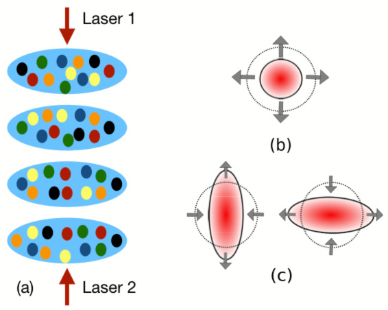
Figure 1: Collective modes of a 2D SU($N$) Fermi gases. (a) Fermionic alkaline-earth atoms can be confined to a single 2D layer or to an array of 2D layers formed by an optical lattice (depicted). Collective modes may be excited, for example by suddenly changing a trap frequency. (b-c) The real space deformations corresponding to the three lowest angular momentum modes, the breathing mode (b), dipole mode (not depicted), and quadrupole mode (c).

II Collective modes and theoretical methods

2D gases can be experimentally realized in ultracold alkaline-earth-like atoms by directly confining them to a single layer (for example with evanescent fields), or by creating an array of 2D systems via a one dimensional optical lattice, as illustrated in Fig. 1(a). We will assume that the lattice is deep enough that the 2D layers are uncoupled. Also, we will assume an isotropic harmonic trap potential with trap frequency $\omega_{\text{tr}}$.

Collective modes may be excited by suddenly changing system parameters. For collective modes of the density, as we consider in this paper, this is often done by suddenly changing a trap frequency by a small amount ($\sim~{}\!10\%)$. Which modes are excited will depend on the symmetry of this perturbation (and of the original trap). A generic perturbation excites a superposition of modes of different symmetry, but often experiments choose perturbations to couple to modes with a single symmetry. For example, an isotropic change of trap frequencies in an isotropic trap excites only breathing modes, illustrated in Fig. 1(b). The other mode we consider in this paper is the quadrupole mode is illustrated in Fig. 1(c). To measure these modes, experiments can track in situ oscillations of the density profile, or oscillations in time-of-flight, which measure the momentum distribution. Sometimes, easier-to-access observables are measured as proxies, for example loss as a function of time, which allows one to measure the frequencies and damping rates, although it provides less details about the spatial and momentum-space mode structure. Recently, He et al. have measured the breathing and quadrupole collective mode frequencies and damping times in SU($N$) Yb gases confined in a one-dimensional lattice, for various $N$ up to $N=6$ He et al. .

A 2D alkaline-earth fermionic gas with $N_{\text{p}}$ particles can be described by the grand canonical Hamiltonian

$$H =\sum_{\alpha}\int\!d^{2}\mathbf{r}\,\psi^{\dagger}_{\alpha}(\mathbf{r})\left(-\frac{\hbar^{2}}{2m}\nabla^{2}-\mu+V(r)\right)\psi_{\alpha}(\mathbf{r})$$

$${}+\frac{g_{2D}}{2}\!\!\sum_{\alpha\neq\beta}\int\!d^{2}\mathbf{r}\,\psi^{\dagger}_{\alpha}(\mathbf{r})\psi^{\dagger}_{\beta}(\mathbf{r})\psi^{\phantom{\dagger}}_{\beta}(\mathbf{r})\psi_{\alpha}^{\phantom{\dagger}}(\mathbf{r}),$$ (1)

where $\psi^{\dagger}_{\alpha}(\mathbf{r})$ is the fermionic creation operator creating an atom at position $\mathbf{r}$ with spin index $\alpha=1,\ldots,N$, $\mu$ is the chemical potential, $m$ is the mass of the atom, $V(r)=m\omega_{\text{tr}}^{2}(x^{2}+y^{2})/2$ is the harmonic trap potential with frequency $\omega_{\text{tr}}$, and $g_{2D}$ is the interaction strength. In principle, this contact interaction must be regularized, but at the level of approximations we use throughout, this will be unnecessary. For a sufficiently deep lattice, so that the potential confining the atoms to the 2D plane can be described by an additive potential $m\omega_{z}^{2}z^{2}/2$ (with $z$ the displacement perpendicular to the plane), the coupling constant is Petrov and Shlyapnikov (2001)

$$g_{2D}=\frac{2\pi\hbar^{2}}{m\ln(qa_{\text{2D}})},$$ (2)

where $a_{\text{2D}}=l_{z}\sqrt{\pi/B}\exp(-\sqrt{\pi/2}l_{z}/a_{\text{3D}})$, $B=0.915$ $a_{\text{3D}}$ is the three-dimensional $s$-wave scattering length, $l_{z}=\sqrt{\hbar/(m\omega_{z})}$, and $q\sim\sqrt{n}$ is a characteristic momentum that determines the density dependent coupling ($n$ being the total density). The momentum factor, $q$ is the Fermi momentum, $k_{F}$ Ghosh and Sinha (2002), and the de Broglie wavelength, $\sqrt{mT}/\hbar$ in the low and high temperature limit respectively Petrov and Shlyapnikov (2001).

We calculate the collective modes by employing two approximations, which are reasonable in the limits considered in this paper. First, we assume that the system is weakly interacting, $1/{\ln{(1/na_{\text{2D}}^{2})}\ll 1}$ (where $n$ is the total density), its temperature is sufficiently high such there is no pairing, and that the length scales over which there is any spatial coherence is small compared to the trap size (though the gas may still be deeply degenerate). In practice this means that the system must be well above the superconducting transition temperature and the length scale on which the collective modes vary must be long compared to the thermal de Broglie wavelength. This allows us to describe the system’s dynamics by a Boltzmann equation, including mean-field interactions in addition to the collision integral, which governs the phase space distribution function (defined later). The resulting Boltzmann-Vlasov (BV) equation   is a 4+1 dimensional partial differential-integral equation, and as such would be extremely demanding to solve numerically.

Second, we approximate the collision integral with a relaxation time approximation. This is an uncontrolled, but standard, approach to calculating transport and collective modes within a Boltzmann equation framework. This approximation will be explained in detail in Sec. III.

To solve the BV equation in the relaxation time approximation, we assume an ansatz for the phase space distribution function. The ansatz is carefully constructed to respect the SO(2,1) symmetry of the system, while simultaneously being flexible enough to capture the collective modes’ shifts and damping. As shown in Ref. Pitaevskii and Rosch (1997), this ansatz provides an exact solution to the collective modes of the BV equation in 2D, when the confinement is isotropic.

Under these assumptions, it is valid to apply mean-field theory to the Hamiltonian in Eq. (II) in the density channel. We assume that the density of each species is the same ($n_{\alpha}=n_{\beta}=n_{0}$, for all $\{\alpha,\beta\}\in\{1,\ldots N\}$), where $n_{0}$ is the density of each species. [This holds in any state that preserves the Hamiltonian’s SU($N$) symmetry.] The mean-field Hamiltonian is then

$$H_{\text{MF}}=\sum_{\alpha}\!\int\!d^{2}\mathbf{r}\,\psi^{\dagger}_{\alpha}(\mathbf{r})\bigg{(}\!-\frac{\hbar^{2}}{2m}\nabla^{2}-\mu+V(r)+U_{\text{MF}}\!\bigg{)}\psi_{\alpha}^{\phantom{\dagger}}(\mathbf{r}),$$ (3)

up to irrelevant constants, and

$$U_{\text{MF}}=g_{\text{2D}}\frac{(N-1)}{N}n^{\text{tot}}(\mathbf{r})$$ (4)

where $n^{\text{tot}}(\mathbf{r})=\sum_{\alpha=1}^{N}n_{\alpha}(\mathbf{r})=Nn_{0}(\mathbf{r})$ is the density of the gas at position $\mathbf{r}$. The chemical potential $\mu$ is chosen to give the total number of particles $N_{p}$ by

$$N_{p}=\int\!d^{2}\mathbf{r}\,n^{\text{tot}}(\mathbf{r})=N\int\!d^{2}\mathbf{r}\,n_{0}(\mathbf{r})$$ (5)

To calculate the collective mode dynamics, we will use the BV kinetic equation, which is a semi-classical method, solved by a scaling ansatz, and linearize for small displacements from equilibrium. The BV kinetic equation is accurate when the conditions outlined above of weak interactions and $k_{\text{B}}T\gg\hbar\omega_{\text{tr}}$ are satisfied. In this limit, we assume that the effects of quantum interference can be neglected, and quasi-particles are well-defined. Furthermore, since our initial state and Hamiltonian are invariant under SU($N$) symmetry (i.e. we are studying the density modes), we have assumed that each spin component is described by the same semi-classical distribution function $f(\mathbf{r},\mathbf{p},t)$ which satisfies BV kinetic equation,

$$\frac{\partial f}{\partial t}+\frac{\textbf{p}}{m}\cdot\frac{\partial f}{\partial\textbf{r}}-\frac{\partial}{\partial\mathbf{r}}\left(V(\mathbf{r})+U_{\text{MF}}(\mathbf{r})\right)\cdot\frac{\partial f}{\partial\textbf{p}}=-I_{\text{coll}}[f],$$ (6)

where $I_{\text{coll}}[f]$ is the collision integral, and $U_{\text{MF}}$ is the mean-field interaction energy. The mean field interaction energy is given by Eq. (4) where the density $n^{\text{tot}}(\mathbf{r})$ is determined from the distribution function by

$$n^{\text{tot}}(\mathbf{r})=N\int\!\frac{d^{2}\mathbf{k}}{(2\pi)^{2}}f(\mathbf{r},\mathbf{k}),$$ (7)

and the collision integral, $I_{\text{coll}}[f]$ is

$$I_{\text{coll}}[f_{1}] =\int\!\frac{d^{2}p_{2}}{(2\pi\hbar)^{2}}\frac{m\hbar}{4\pi}\int_{0}^{2\pi}\!d\theta|\mathcal{T}(|{\mathbf{p}_{r}}|)|^{2}(N-1)$$

$${}\times\left[f_{1}f_{2}(1-f_{3})(1-f_{4})-f_{3}f_{4}(1-f_{1})(1-f_{2})\right],$$

where we define $f_{j}=f(\mathbf{r},\mathbf{p}_{j})$, and $\mathbf{p}_{3}$ and $\mathbf{p}_{4}$ are given in terms of $\mathbf{p}_{1}$, $\mathbf{p}_{2}$, and $\theta$ as follows: $\theta$ is the angle between the outgoing relative angular momentum $\mathbf{p}_{r}=(\mathbf{p}_{3}-\mathbf{p}_{4})/2$ and the center of mass momentum, ($\mathbf{p}_{1}+\mathbf{p}_{2}$), $\mathbf{p}_{4}$ is given by conservation of the center-of-mass momentum $\mathbf{p}_{3}+\mathbf{p}_{4}=\mathbf{p}_{1}+\mathbf{p}_{2}$, and by the conservation of energy we obtain $|\mathbf{p}_{r}|=|\mathbf{p}_{r}^{\prime}|$, where $\mathbf{p}_{r}^{\prime}=(\mathbf{p}_{1}-\mathbf{p}_{2})/2$. The low energy $T$-matrix describing the collision between two atoms with different spins in 2D (in the vacuum) is given by Landau and Lifshitz (2013):

$$\mathcal{T}(q)=\frac{4\pi}{m}\frac{1}{\ln{(1/q^{2}a_{\text{2D}}^{2})}+i\pi}.$$ (9)

It is hard to solve the BV equation exactly, even numerically, since this is 5 dimensional partial integro-differential equation. In this paper, we employ a scaling ansatz for $f(\mathbf{r},\mathbf{p},t)$ Guéry-Odelin (2002); Pedri et al. (2003); Dong et al. (2015); Wächtler et al. (2017). Our ansatz $f_{sc}$ is defined as

$$f_{sc}(\mathbf{r},\mathbf{v},t)=\Gamma(t)f^{0}(\mathbf{R}(t),\mathbf{V}(t))$$ (10)

where $R_{i}(t)=\frac{r_{i}}{b_{i}(t)},V_{i}=\frac{1}{\sqrt{\theta_{i}(t)}}\left(v_{i}-\frac{\dot{b}_{i}(t)}{b_{i}(t)}r_{i}\right)$, and $\Gamma(t)=\frac{1}{\prod_{i=1}^{2}b_{i}(t)\sqrt{\theta_{i}(t)}}$, where $b_{i}$ and $\theta_{i}$ are functions of time that will be determined to give the best solution to the BV equation. The equilibrium distribution function, $f^{0}$, is defined by $I_{\text{coll}}[f^{0}]=0$, which gives

$$m\textbf{v}\cdot\frac{\partial f^{0}}{\partial\textbf{r}}=\frac{\partial}{\partial\mathbf{r}}(V(r)+U_{\text{MF}})\cdot\frac{\partial f^{0}}{\partial\textbf{v}}.$$ (11)

As mentioned, the scaling ansatz respects the classical SO$(2,1)$ scaling symmetry. Quantum effects can lead to a breaking of this symmetry and an anomalous correction to the breathing mode frequency. A calculation of this quantum anomaly is beyond the scope of the BV equation, and we restrict our calculations to the regime where the BV equation is valid.

Additionally, we treat the collision integral in the relaxation time approximation,

$$I_{\text{coll}}[f]=\frac{f-f^{0}}{\tau},$$ (12)

where $\tau$ is the relaxation time of the collision, which is calculated in Sec. III.2.

III Results

In this section, we will compute the collective mode frequencies (Sec. III.1) and damping rates (Sec. III.2) of the SU($N$) Fermi gas. We find that the breathing mode frequency has no dependence on the interaction strength, reflecting the SO(2,1) symmetry of the system at the classical level. However, the quadrupole mode frequencies exhibit an interaction dependent shift, and damping. We discuss how this shift and damping rates depend on $N$, and estimate the values of these quantities for reasonable experimental parameters.

III.1 Collective mode frequencies

Following Ref. Pedri et al. (2003), we compute the average moments of $R_{i}V_{i}$ and $V_{i}^{2}$ and obtain the following equations for $b_{i}$ and $\theta_{i}$:

$$\ddot{b_{i}}+\omega_{\text{tr}}^{2}b_{i}-\omega_{\text{tr}}^{2}\frac{\theta_{i}}{b_{i}}+\omega_{\text{tr}}^{2}\xi\left(\frac{\theta_{i}}{b_{i}}-\frac{1}{b_{i}\prod_{j}b_{j}}\right) =0$$ (13)

$$\dot{\theta_{i}}+2\frac{\dot{b}_{i}}{b_{i}}\theta_{i}=-\frac{\theta_{i}-\bar{\theta}}{\tau}$$ , (14)

where $i\in\{x,y\}$, $\bar{\theta}=\frac{1}{2}\sum_{i}\theta_{i}$, and

$$\xi=\frac{\langle U_{\text{MF}}\rangle}{\langle m\omega_{\text{tr}}^{2}(x^{2}+y^{2})\rangle}$$ (15)

where $\langle\cdots\rangle=\int\!d^{2}\mathbf{r}\!\int\!\frac{d^{2}\mathbf{k}}{\left(2\pi\right)^{2}}f^{0}\left(\cdots\right)$. For the remainder of this section, we give our results in terms of $\xi$ and $\tau$. We will then calculate $\xi$ and $\tau$ in terms of system parameters in Sec. III.2.

We linearize Eqs. (13) and (14) around the equilibrium values $\left(b_{i}=1+\delta b_{i},\theta_{i}=1+\delta\theta_{i}\right)$ to get the collective mode frequencies of the density oscillations. We obtain

$$\ddot{\delta b}_{j}+\omega_{\text{tr}}^{2}(2+\xi)\delta b_{j}+\xi\omega_{\text{tr}}^{2}\delta b_{\bar{\jmath}}+\omega_{\text{tr}}^{2}(\xi-1)\delta\theta_{j}=0$$ (16)

$$\dot{\delta\theta}_{j}+2\dot{\delta b_{j}}+\frac{1}{2\tau}(\delta\theta_{j}-\delta\theta_{\bar{\jmath}})=0$$ (17)

with ${\bar{\jmath}}=x$ if $j=y$, and ${\bar{\jmath}}=y$ if $j=x$. The collective modes have solutions of the form $\delta b_{i}(t)=b_{i}^{0}e^{i\omega t}$ and $\delta\theta_{i}(t)=\theta_{i}^{0}e^{i\omega t}$. Substituting into the above equations, we obtain a set of four linear equations for $b_{i}^{0}$ and $\theta_{i}^{0}$, which have non-zero solutions when the determinant of the associated matrix is zero. This gives a polynomial equation in $\omega$ that can be written

$$\omega^{2}(\omega^{2}-\omega_{\text{Br}}^{2})\left[\left(\omega^{2}-\omega_{\text{cl}}^{2}\right)-\frac{i}{\omega\tau}\left(\omega^{2}-\omega_{\text{hd}}^{2}\right)\right]=0,$$ (18)

with $\omega_{\text{Br}}=2\omega_{\text{tr}}$, $\omega_{\text{hd}}=\sqrt{2}\omega_{\text{tr}},$ and $\omega_{\text{cl}}=\sqrt{2(2-\xi)}\omega_{\text{tr}}$.

The solution $\omega=\omega_{\text{Br}}$ to Eq. (18) corresponds to the breathing mode. It is purely real, and it is independent of $\xi$ and $\tau$, and hence independent of all system parameters other than $\omega_{\text{tr}}$. As mentioned this is a consequence of the scaling symmetry of the system. In the future it will be interesting to investigate the effects of the breakdown of this symmetry due to quantum effects.

The solutions to the term in brackets in Eq. (18), $\left(\omega^{2}-2(2-\xi)\omega_{\text{tr}}^{2}\right)-\frac{i}{\omega\tau}\left(\omega^{2}-2\omega_{\text{tr}}^{2}\right)=0$, give the quadrupole modes’ (complex) resonance frequencies. In the hydrodynamic limit, $\omega_{\text{tr}}\tau\rightarrow 0$, the solution is $\omega=\omega_{\text{hd}}=\sqrt{2}\omega_{\text{tr}}$, and in the collisionless limit, $\omega_{\text{tr}}\tau\rightarrow\infty$, the solution is $\omega=\omega_{\text{cl}}=\sqrt{2(2-\xi)}\omega_{\text{tr}}$. The real part of the frequency smoothly crosses over between these two limits [see Fig. 2(a)] while the imaginary part is zero in these two limits, peaking in between [see Fig. 2(b)].

This behavior of the imaginary part of $\omega$ is very general, and can be understood using the following argument. In the hydrodynamic limit $\omega\tau\ll 1$, there is no dissipation since frequent collisions force the deviations from local thermodynamic equilibrium, which are necessary for dissipation, to be negligible Pethick and Smith (2008). In this limit, the collective mode frequency is:

$$\omega=\omega_{\text{h}d}-i\frac{\tau(\omega_{\text{c}l}^{2}-\omega_{\text{h}d}^{2})}{2}.$$ (19)

On the other hand, in the collisionless limit $\omega\tau\gg 1$, there are few collisions per oscillation period, so dissipation is again negligible. In this limit, the collective mode frequency is:

$$\omega=\omega_{\text{c}l}-i\frac{\omega_{\text{c}l}^{2}-\omega_{\text{h}d}^{2}}{2\tau\omega_{\text{c}l}^{2}}.$$ (20)

It is clear that the damping rate must peak somewhere between the collisionless and hydrodynamic limits. Numerically, we find that the peak occurs, when $\omega\tau\sim 1$.

As detailed in Appendix A, $\xi$ is given by

$$\xi=\frac{g_{\text{2D}}(N-1)}{2\frac{\pi\hbar^{2}}{m}}F(\frac{T}{\hbar\omega_{\text{tr}}},\frac{N_{p}}{N}),$$ (21)

where $F(\frac{T}{\hbar\omega_{\text{tr}}},\frac{N_{p}}{N})$ is defined as the ratio of one-dimensional integrals in Eq. (56) and in general can be evaluated numerically. In this calculation, we have ignored the mean-field contribution to the equilibrium distribution function, $f^{0}$. This approximation gives the value of $\xi$ to the leading order in $g_{\text{2D}}$. It is possible to evaluate $\xi$ analytically in the low temperature and high temperature limits. In the low temperature limit, when $T\ll T_{F}$, $\xi$ is

$$\xi=\frac{g_{2D}m}{2\pi\hbar^{2}}(N-1).$$ (22)

In the high temperature limit, when $T\gg T_{F}$, $\xi$ is

$$\xi=\frac{1}{8\pi}\frac{g_{\text{2D}}(N-1)}{\frac{\hbar^{2}}{m}}\frac{N_{p}}{N}\left(\frac{\hbar\omega_{\text{tr}}}{T}\right)^{2}.$$ (23)

It is interesting to note that commonly-employed alternative approaches to computing the collective mode frequencies for a 2D SU($2$) Fermi gas have neglected the mean-field contribution Baur et al. (2013); Chiacchiera et al. (2013). Due to this approximation, neither the breathing mode, nor the quadrupole modes show any mean-field shift in these calculations. Moreover, including the mean-field contribution in the Boltzmann equation in these approaches leads to an unphysical shift in the breathing mode frequency due to the improper treatment of the SO(2,1) symmetry. As shown in the recent experiment by He et al. He et al. , accounting for the mean-field shifts in the quadrupole mode can be important, especially as $N$ increases. Our approach captures the mean-field effects while not inducing an unphysical shift in the breathing mode frequency.

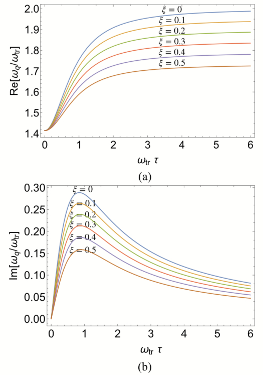
Figure 2: Scaled quadrupole mode frequency($\frac{\omega_{q}}{\omega_{\text{tr}}}$) vs scaled scattering time $\omega_{\text{tr}}\tau$. (a) Real part of the mode frequency vs scattering time, (b) imaginary part of the mode frequency vs scattering time.

III.2 Damping Rate Calculation

In this section, we outline our calculations for the relaxation time $\tau$, which employs a few common approximations. Following Ref. Baur et al. (2013), we write $f({\bf r,p})=f_{0}({\bf r,p})+\left[f_{0}({\bf r,p})(1-f_{0}({\bf r,p}))\right]\phi({\bf r,p})$. Rearranging and taking moments of Eq. (12), the relaxation time is given by

$$\frac{1}{\tau}=\frac{\langle\phi^{*}I_{\text{coll}}[\phi]\rangle}{\langle|\phi|^{2}f^{0}(1-f^{0})\rangle}.$$ (24)

To evaluate the relaxation rate, we use the following ansatz for $\phi({\bf r,p})$:

$$\phi=p_{x}^{2}-p_{y}^{2}.$$ (25)

The linearized collision integral then reads:

$$I_{\text{coll}}[f_{1}]= \int\!\frac{d^{2}p_{2}}{(2\pi\hbar)^{2}}\frac{m\hbar}{4\pi}\int_{0}^{2\pi}\!d\theta|\mathcal{T}|^{2}(\phi_{1}+\phi_{2}-\phi_{3}-\phi_{4})$$ (26)

$$\hskip 14.45377pt{}\times f_{1}f_{2}(1-f_{3})(1-f_{4})(N-1)$$

The calculations are easiest in the high temperature limit, when the Pauli blocking factors can be ignored. For weakly interacting Fermi gases, this approach overestimates the damping rate (by about $50\%$) for typical experimental temperatures ($T\sim 0.5T_{F}$) Baur et al. (2013). We note that even in an anisotropic trap, this approximation gives a lower bound on the relaxation time in the weakly interacting limit.

A more accurate estimate of the damping rate can be obtained by accounting for the Pauli blocking. This approach involves solving a six dimensional integral numerically, and overestimates the damping rate by about $10\%$ for $N=2$. It is possible to further systematically improve the damping rate estimate, by using ansatz for the function $\phi$ that are more flexible than Eq. (25). Using a sufficiently complete basis, the result will converge to the true damping rate (within the relaxation time approximation). The damping rate obtained using this technique is always bounded from below by the actual damping rate Pethick and Smith (2008); Enss et al. (2012), so convergence may be monitored as the damping tends to its minimum, in a manner analogous to other variational calculations, e.g. the convergence of the energy to its minimum when calculating the quantum mechanical ground state energy.

The relaxation time in this high temperature limit is found to be

$$\frac{1}{\tau} = \frac{N-1}{\tau_{0}}$$ (27)

where

$$\frac{1}{\tau_{0}}=\frac{\pi N_{p}(\hbar\omega_{\text{tr}})^{2}}{2N\hbar k_{B}T}G\left(\frac{\hbar^{2}}{ma_{\rm 2D}^{2}k_{B}T}\right)$$ (28)

and

$$G(x)=\int_{0}^{\infty}dz\frac{z^{2}\exp(-z)}{\ln{(x/z)}^{2}+\pi^{2}}.$$ (29)

III.3 Experimental implications

In this subsection, we compute the values of the mean-field shifts of the quadrupole modes and the damping rates for realistic experimental parameters. Following He et al. He et al. , we use the parameters $T=60\,\text{nK}$, $T/T_{F}=0.42$, $\omega_{z}=2\pi\times 59\,$kHz, $\omega_{\text{tr}}=2\pi\times 185\,$Hz, $N_{p}/N=100$, $T/\hbar\omega_{\text{tr}}=5.94$, $\ln(k_{F}a_{\text{2D}})=-4.3$ to estimate the quadrupole mode shifts and the damping rates. For these parameters, the interaction strength is

$$\frac{g_{\text{2D}}}{\frac{\hbar^{2}}{m}}=-\frac{2\pi}{\ln(k_{F}a_{\text{2D}})}=1.461.$$ (30)

Using Eq.(56), $\xi$, the parameter controlling the mean field shift, is then

$$\xi=\frac{g_{\text{2D}}}{2\pi\frac{\hbar^{2}}{m}}(N-1)F(5.94,100)\approx 0.093(N-1)$$ (31)

We compute the damping rate using Eq. (27), finding

$$\frac{1}{\tau}\approx 0.095(N-1)\frac{k_{B}T}{\hbar}.$$ (32)

Fig. 3 shows the collective mode frequency shifts and damping for the experimental parameters of Ref. He et al. as a function of $N=1\ldots 6$. Our results for both the shifts and damping agree qualitatively with the experimental data presented in Ref. He et al. . Our prediction of the frequency shift is close to the experimentally observed frequency shift when $N=2$. We overestimate the frequency shift when $N\geq 3$, and our prediction for $\omega_{\text{c}l}$ is about $10\%$ less than the experimentally observed value when $N=6$. This discrepancy is likely due to our approximation of retaining fully only the leading order contribution of $g_{\text{2}D}$ to the frequency shift, by neglecting the mean-field effects in the equilibrium distribution function. For larger $N$, a better estimate of $\xi$ can be obtained by including these mean-field effects He et al. . Our damping rate estimate shows an increase in damping rate with $N$, as observed experimentally. It is about $50\%$ larger than the observed damping rate when $N=2$. This is in agreement with previous calculations Baur et al. (2013), and is in reasonable agreement with experiment after accounting for uncertainties in experimental parameters. However, for $N=6$, our estimate of the damping rate is roughly a factor of four larger than the measurements. It will be interesting to explore in future work to what extent this discrepancy results from uncertainties in experimental parameters and to what extent it is from approximations employed in the theory.

The presence of an anisotropic trap generally leads to a coupling of the breathing and quadrupole modes Baur et al. (2013). This leads to a decay of the breathing mode. However, the anisotropy in recent experiments is negligible (less than $1\%$) He et al. , and therefore we do not consider the effects of anisotropy in this paper.

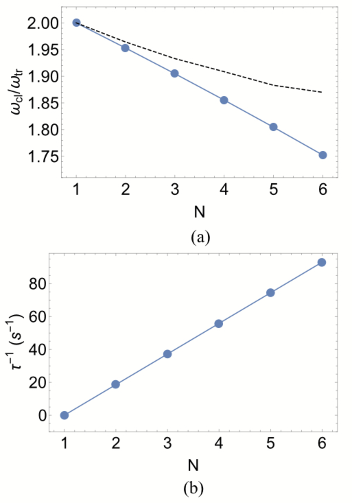
Figure 3: (a) The ratio of the quadrupole mode frequency to the trap frequency in the collisionless limit. The solid blue line, and the dashed black line show the value of this ratio to exactly leading order in $g_{\text{2}D}$ (neglecting the mean-field changes of the equilibrium distribution function $f^{0}$), and including the effects of mean-field interactions in $f^{0}$, respectively. (b) The damping rate of the quadrupole modes, $\tau^{-1}$ (in units of $s^{-1}$) for parameters corresponding to the experiment in Ref. He et al.

III.4 3D results

The previous subsections computed the frequencies and damping rates of the collective modes of the 2D SU($N$) Fermi gas. We now briefly discuss the situation when there is no potential to confine the system to be two dimensional (e.g. no lattice), and only a weak trapping potential in that direction. For our calculations, we assume that the gas is confined in a cylindrically symmetric harmonic potential, where $\omega_{x}=\omega_{y}=\omega_{\perp}$, and $\omega_{z}=\lambda\omega_{\perp}$. As outlined in Ref. Pedri et al. (2003), the quadrupole mode frequencies are determined by the equation:

$$(\omega^{2}-\omega_{\rm cl}^{2})+\frac{i}{\omega\tau}(\omega^{2}-\omega_{\rm hd}^{2})=0,$$ (33)

where $\omega_{\rm cl}^{2}=2\omega_{\perp}^{2}(2-\xi)$ and $\omega_{\rm hd}^{2}=2\omega_{\perp}^{2}$, where the frequency shift $\xi$ is given by:

$$\xi=g(N-1)\frac{\langle n(r)\rangle}{\langle 2m\omega_{i}^{2}r_{i}^{2}\rangle}=\frac{g(N-1)}{N}\frac{3\langle n^{\rm tot}(r)\rangle}{\langle 2m\omega_{\perp}^{2}\rho^{2}\rangle},$$ (34)

where $\rho=\sqrt{x^{2}+y^{2}+\lambda^{2}z^{2}}$. We compute the collective mode frequencies in the low-temperature limit, where analytical results can be obtained. At zero temperature, the total density $n^{\rm tot}(r)$ can be approximated to be:

$$n^{\rm tot}(r)=\frac{8N_{p}\lambda}{\pi^{2}R_{F}^{3}}(1-\frac{\rho^{2}}{R_{F}^{2}})^{3/2}\Theta(R_{F}-r)$$ (35)

where $R_{F}=(48N_{p}\lambda)^{1/6}\sqrt{\hbar/(m\omega_{\perp})}$ Butts and Rokhsar (1997). Thus the shift, $\xi$ is given by:

$$\xi = \frac{g(N-1)}{N}\frac{12N_{p}\lambda}{m\omega_{\perp}^{2}\pi^{2}R_{F}^{3}}\frac{\int d^{3}r(1-\frac{\rho^{2}}{R_{F}^{2}})^{3}\Theta(R_{F}-r)}{\int d^{3}r\rho^{2}(1-\frac{\rho^{2}}{R_{F}^{2}})^{3/2}\Theta(R_{F}-r)}$$ (36)

$$= \frac{g(N-1)}{m\omega_{\perp}^{2}R_{F}^{2}N}\frac{\sqrt{3N_{p}\lambda(m\omega_{\perp})^{3}}}{\pi^{2}\hbar^{3/2}}\frac{4096}{945\pi}.$$

IV Conclusions

We have calculated the collective modes for density oscillations of a harmonically-trapped 2D SU($N$) Fermi gas, carefully incorporating the SO(2,1) scaling symmetry. We employed a Boltzmann-Vlasov equation, which is valid for weak interactions and when the system is large compared to spatial coherences. We treated the collisions within the relaxation time approximation, which, while an uncontrolled approximation, is standard and captures the essential features of the hydrodynamic (and collisionless) limits. We solved this using a scaling ansatz, Eq. (10), for the semiclassical distribution function $f(\mathbf{r},\mathbf{p})$. In contrast to other methods, for example those based on the method of moments  Guéry-Odelin et al. (1999); Ghosh (2000); Bruun and Smith (2007); Chiacchiera et al. (2011), the scaling ansatz preserves the SO(2,1) scaling symmetry, while also being flexible enough to allow for mean-field shifts.

We have shown that the magnitude of the shifts are sufficiently large to measure if the system is confined in one dimension by an optical lattice. This suggestion is borne out in recent experiments that were carried out as this manuscript was being finalized He et al. . We note that in the collisionless limit, our calculations of shifts are equivalent to theirs, but ours apply across the full collisionless-hydrodynamic crossover, and also capture the mode damping.

The predicted quadrupole mode shifts agree with Ref. He et al. ’s experimental measurements after accounting for uncertainty in the experimental parameters. The predicted damping rate agrees with the order of magnitude observed in the experiments. For $N=2$, the damping rates agree with about $30\%$ relative error. However, for $N=6$ the predicted damping rate is roughly four times the experimentally measured rate. It is possible that this arises from uncertainties in experimental parameters, which lead to a significant uncertainty already in the collective mode shift frequencies. It’s also possible that it arises from the approximations inherent in deriving and solving the BV equation. An interesting future direction will be precision experiments and calculations to pinpoint the reason for the discrepancy.

Besides calculating the weakly interacting gases’ collective modes, the results in this paper lay the groundwork for several future directions with ultracold SU($N$) gases collective modes and transport. One direction is to explore strongly interacting gases, for instance to understand the shear viscosity Enss et al. (2012) or search for novel Fermi liquid behaviors and instabilities Yip et al. (2014); Cheng and Yip (2017); How and Yip (2018). A strongly interacting regime may be achieved by tighter transverse confinement, higher densities, or optical Feshbach resonance Blatt et al. (2011); Yan et al. (2013); Nicholson et al. (2015). In strongly interacting gases, the scaling anomaly should cause measurable effects, especially collective mode frequency shifts, and the ability to tune $N$ will shed new light into its effects. In this regard, it will be interesting to employ other, sensitive probes of the scale anomaly, for example the momentum-space dynamics Murthy et al. . It will also be interesting to study physics at lower temperatures, especially when the system becomes superfluid. Although the present calculations are performed for weakly interacting normal gases, such calculations form an important point of comparison for strongly interacting and superfluid gases.

Another direction would be to explore the spin modes Enss and Haussmann (2012); Enss (2013), which could allow a new window into strongly correlated spin transport. These modes have been explored in $N=2$ alkali gases Koschorreck et al. (2013); Bardon et al. (2014); Trotzky et al. (2015); Valtolina et al. (2017); Enss and Thywissen (2019), but the potential spin structures are richer for larger $N$. A scaling ansatz similar in spirit to our approach, with a spin dependent distribution function $f_{\sigma}({\bf r},{\bf p},t)$ has already been used to study spin dipole modes for $SU(2)$ fermi gases Vichi and Stringari (1999); Sommer et al. (2011). Furthermore, it may be possible to generalize this scaling ansatz to include coherences. Thus, we expect that this technique can shed light on the spin collective modes of $SU(N)$ gases as well.

Appendix A Calculation of $\xi$

Using Eqs. (4) and (15) we have

$$\xi=\frac{g_{\text{2D}}(N-1)}{m\omega_{\text{tr}}^{2}N}\frac{\int d^{2}\mathbf{r}n^{\text{tot}}(\mathbf{r})^{2}}{\int d^{2}\mathbf{r}n^{\text{tot}}(\mathbf{r})r^{2}}.$$ (37)

To calculate $\xi$, we need to know the form of equilibrium spatial density $n^{\text{tot}}(\mathbf{r})$ at a chemical potential set to match the total number of particles given by Eq. (5):

$$N_{p}=\int d^{2}\mathbf{r}n^{\text{tot}}(\mathbf{r})=N\int d^{2}\mathbf{r}\int\frac{d^{2}\mathbf{p}}{\left(2\pi\right)^{2}}f^{0}(\mathbf{r},\mathbf{p},\mu,T),$$ (38)

where

$$f^{0}=\frac{1}{e^{\left(\frac{p^{2}}{2m}+V(\mathbf{r}+U_{\text{M}F})-\mu\right)/T}+1}.$$ (39)

The chemical potential $\mu$ is determined by fixing $N_{p}=\int d^{2}{\bf r}n^{\text{tot}}(\mathbf{r})$. We can then numerically evaluate $\xi$ in Eq. (37) for the total particle number $N_{p}$ at a temperature $T$, and trap frequency $\omega$. The mean-field contribution to $f^{0}$ can be ignored in the weakly interacting regime, since it only changes the density perturbatively. In the following analysis, we set $U_{\text{M}F}=0$. One can show that Eq. (38) can be written as,

$$\frac{N_{p}}{N}\left(\hbar\omega_{\text{tr}}\right)^{2}=\int\frac{dvdu}{e^{\beta(v+u-\mu)}+1}=-\frac{\operatorname{Li}_{2}(-e^{\beta\mu})}{\beta^{2}}$$ (40)

where $\operatorname{Li}_{\alpha}(z)$ is the polylog function.

In general this equation can be solved numerically, as discussed in Sec. A.3. In the next subsections we analytically solve it in the high- and low-temperature limits.

A.1 Low Temperature limit $T\ll\hbar\omega_{\text{tr}}\sqrt{2\frac{N_{p}}{N}}$

For $T\rightarrow 0$, we have

$$\frac{N_{p}}{N}\left(\hbar\omega_{\text{tr}}\right)^{2} =\int_{0}^{\infty}\!dv\int_{0}^{\infty}\!du\,\Theta(\mu-(v+u))$$ (41)

$$=\frac{\mu(T=0)^{2}}{2}$$ (42)

$$=\frac{E_{F}^{2}}{2},$$ (43)

where $\Theta$ is the Heaviside theta function and $E_{F}$ is the Fermi energy,

$$E_{F}=\hbar\omega_{\text{tr}}\sqrt{2\frac{N_{p}}{N}}.$$ (44)

The density is

$$n^{\text{tot}}(\mathbf{r})=N\int\frac{d^{2}\mathbf{k}}{\left(2\pi\right)^{2}}f^{0}=\frac{N}{2\pi}\frac{m}{\hbar^{2}}\int ds\frac{1}{e^{\beta(s+V(\mathbf{r})-\mu}+1},$$ (45)

which at low temperature is

$$n^{\text{tot}}(\mathbf{r})=\frac{N}{2\pi}\frac{m}{\hbar^{2}}\left(E_{F}-V(\mathbf{r})\right)\Theta\left(E_{F}-V(\mathbf{r})\right).$$ (46)

Using the expression for $E_{F}$ and $V(\mathbf{r})$, we get,

$$n^{\text{tot}}(\mathbf{r})=\frac{N}{4\pi}\frac{r_{0}^{2}-r^{2}}{l^{4}}\Theta(r_{0}-r)$$ (47)

where $r_{0}=l\left(8\frac{N_{p}}{N}\right)^{\frac{1}{4}}$ and $l=\sqrt{\frac{\hbar}{m\omega_{\text{tr}}}}$. Using Eqs. (47) and (37), at low temperature($T\ll E_{F}$) we find

$$\xi=\frac{g_{\text{2D}}(N-1)}{\frac{2\pi\hbar^{2}}{m}}.$$ (48)

A.2 High temperature limit $T\gg\hbar\omega_{\text{tr}}\frac{N_{p}}{N}$

At high temperature,

$$\frac{N_{p}}{N}\left(\hbar\omega_{\text{tr}}\right)^{2} =\int\!\frac{dvdu}{e^{\beta(v+u-\mu)}+1}$$ (49)

$$\approx\int\!dvdu\,e^{\beta(\mu-v-u)}$$ (50)

$$=\frac{1}{\beta^{2}}e^{\beta\mu}$$ (51)

so

$$\mu=T\log\left(\frac{N_{p}}{N}\left(\frac{\hbar\omega_{\text{tr}}}{T}\right)^{2}\right).$$ (52)

This approximation is only true when $e^{-\beta\mu}\gg 1\rightarrow T\gg\hbar\omega_{\text{tr}}\frac{N_{p}}{N}$. With this approximation, at high temperature density becomes,

$$n^{\text{tot}}(\mathbf{r})=\frac{N_{p}}{2\pi}\frac{\hbar\omega_{\text{tr}}}{T}\frac{e^{-\beta V(\mathbf{r})}}{l^{2}}$$ (53)

and,

$$\xi=\frac{1}{8\pi}\frac{g_{\text{2D}}(N-1)}{\frac{\hbar^{2}}{m}}\frac{N_{p}}{N}\left(\frac{\hbar\omega_{\text{tr}}}{T}\right)^{2}.$$ (54)

A.3 Scaling analysis

Eq. (40) implies that $\tilde{\mu}=S(\frac{N_{p}}{N},\tilde{T})$, where $\tilde{\mu}\equiv\frac{\mu}{\hbar\omega_{\text{tr}}}$, $\tilde{T}\equiv\frac{T}{\hbar\omega_{\text{tr}}}$, and $S=-\tilde{T}\log[\operatorname{Li}_{2}^{-1}[-\frac{N_{p}}{N}\frac{1}{\tilde{T}^{2}}]]$. The density is

$$n^{\text{tot}}(\mathbf{r})=\frac{N}{2\pi}\frac{m}{\hbar^{2}}\int ds\frac{1}{e^{\beta(s+V(\mathbf{r})-\mu}+1}\\ =\frac{N}{2\pi}\frac{1}{l^{2}}\int d\tilde{s}\frac{1}{e^{\frac{\tilde{s}}{\tilde{T}}}e^{\left(\frac{r}{l}\right)^{2}\frac{1}{2\tilde{T}}}e^{-\frac{\tilde{\mu}}{\tilde{T}}}+1}=\frac{N}{2\pi l^{2}}h(\frac{r}{l},\tilde{T},\frac{N_{p}}{N}),$$ (55)

implicitly defining $h$ on the last line. Scaling Eq. (37), $\xi$ is given by

$$\xi =\frac{g_{\text{2D}}(N-1)}{2\pi m\omega_{\text{tr}}^{2}l^{4}}\frac{\int d^{2}\mathbf{r}h(r,\tilde{T},\frac{N_{p}}{N})^{2}}{\int d^{2}\mathbf{r}r^{2}h(r,\tilde{T},\frac{N_{p}}{N})}$$ (56)

$$=\frac{g_{\text{2D}}(N-1)}{\frac{2\pi\hbar^{2}}{m}}F(\tilde{T},\frac{N_{p}}{N})$$ (57)

$$=\xi_{0}F(\tilde{T},\frac{N_{p}}{N}).$$ (58)

Here $F$ is implicitly defined in the second line, and $\xi_{0}=\frac{g_{\text{2D}}(N-1)}{\frac{\pi\hbar^{2}}{m}}$. One can numerically calculate $F(\tilde{T},\frac{N_{p}}{N})$ in general, while the prior two sections show that $F(0,\frac{N_{p}}{N})=1$ and $F(\tilde{T}\gg\frac{N_{p}}{N},\frac{N_{p}}{N})=\frac{1}{4}\frac{N_{p}}{N}\frac{1}{\tilde{T}^{2}}$.

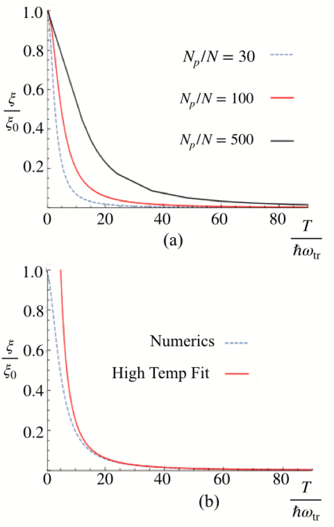
Figure 4: (a)$\frac{\xi}{\xi_{0}}$ vs $\frac{T}{\hbar\omega_{\text{tr}}}$ for different values of $\frac{N_{p}}{N}$ and (b) Numerical calculation for $\frac{\xi}{\xi_{0}}$ vs theoretical calculation at high temperature limit for $\frac{N_{p}}{N}=100$.

References

- Daley (2011) A. J. Daley, Quantum Information Processing 10, 865 (2011).
- Stellmer et al. (2014) S. Stellmer, F. Schreck, and T. C. Killian, “Degenerate quantum gases of strontium,” in Annual Review of Cold Atoms and Molecules (World Scientific, 2014) Chap. 1, pp. 1–80.
- Cazalilla and Rey (2014) M. A. Cazalilla and A. M. Rey, Reports on Progress in Physics 77, 124401 (2014).
- He et al. (2019) C. He, E. Hajiyev, Z. Ren, B. Song, and G.-B. Jo, Journal of Physics B: Atomic, Molecular and Optical Physics 52, 102001 (2019).
- Wu et al. (2003) C. Wu, J.-P. Hu, and S.-C. Zhang, Phys. Rev. Lett. 91, 186402 (2003).
- Cazalilla et al. (2009) M. A. Cazalilla, A. F. Ho, and M. Ueda, New Journal of Physics 11, 103033 (2009).
- Gorshkov et al. (2010) A. V. Gorshkov, M. Hermele, V. Gurarie, C. Xu, P. S. Julienne, J. Ye, P. Zoller, E. Demler, M. D. Lukin, and A. M. Rey, Nature Physics 6, 289 (2010).
- Stellmer et al. (2011) S. Stellmer, R. Grimm, and F. Schreck, Phys. Rev. A 84, 043611 (2011).
- Zhang et al. (2014) X. Zhang, M. Bishof, S. L. Bromley, C. V. Kraus, M. S. Safronova, P. Zoller, A. M. Rey, and J. Ye, Science 345, 1467 (2014).
- Hermele et al. (2009) M. Hermele, V. Gurarie, and A. M. Rey, Phys. Rev. Lett. 103, 135301 (2009).
- Hermele and Gurarie (2011) M. Hermele and V. Gurarie, Phys. Rev. B 84, 174441 (2011).
- Honerkamp and Hofstetter (2004) C. Honerkamp and W. Hofstetter, Phys. Rev. Lett. 92, 170403 (2004).
- Gorelik and Blümer (2009) E. V. Gorelik and N. Blümer, Phys. Rev. A 80, 051602(R) (2009).
- Tóth et al. (2010) T. A. Tóth, A. M. Läuchli, F. Mila, and K. Penc, Phys. Rev. Lett. 105, 265301 (2010).
- Rapp and Rosch (2011) A. Rapp and A. Rosch, Phys. Rev. A 83, 053605 (2011).
- Manmana et al. (2011) S. R. Manmana, K. R. A. Hazzard, G. Chen, A. E. Feiguin, and A. M. Rey, Phys. Rev. A 84, 043601 (2011).
- Corboz et al. (2011) P. Corboz, A. M. Läuchli, K. Penc, M. Troyer, and F. Mila, Phys. Rev. Lett. 107, 215301 (2011).
- Hazzard et al. (2012) K. R. A. Hazzard, V. Gurarie, M. Hermele, and A. M. Rey, Phys. Rev. A 85, 041604(R) (2012).
- Bonnes et al. (2012) L. Bonnes, K. R. A. Hazzard, S. R. Manmana, A. M. Rey, and S. Wessel, Phys. Rev. Lett. 109, 205305 (2012).
- Messio and Mila (2012) L. Messio and F. Mila, Phys. Rev. Lett. 109, 205306 (2012).
- Bauer et al. (2012) B. Bauer, P. Corboz, A. M. Läuchli, L. Messio, K. Penc, M. Troyer, and F. Mila, Phys. Rev. B 85, 125116 (2012).
- Inaba and Suga (2013) K. Inaba and S.-I. Suga, Modern Physics Letters B 27, 1330008 (2013).
- Sotnikov and Hofstetter (2014) A. Sotnikov and W. Hofstetter, Phys. Rev. A 89, 063601 (2014).
- Nataf and Mila (2014) P. Nataf and F. Mila, Phys. Rev. Lett. 113, 127204 (2014).
- Sotnikov (2015) A. Sotnikov, Phys. Rev. A 92, 023633 (2015).
- Nataf et al. (2016a) P. Nataf, M. Lajkó, P. Corboz, A. M. Läuchli, K. Penc, and F. Mila, Phys. Rev. B 93, 201113(R) (2016a).
- Chen et al. (2016) G. Chen, K. R. A. Hazzard, A. M. Rey, and M. Hermele, Phys. Rev. A 93, 061601(R) (2016).
- Capponi et al. (2016) S. Capponi, P. Lecheminant, and K. Totsuka, Annals of Physics 367, 50 (2016).
- Nataf et al. (2016b) P. Nataf, M. Lajkó, A. Wietek, K. Penc, F. Mila, and A. M. Läuchli, Phys. Rev. Lett. 117, 167202 (2016b).
- Hofrichter et al. (2016) C. Hofrichter, L. Riegger, F. Scazza, M. Höfer, D. R. Fernandes, I. Bloch, and S. Fölling, Phys. Rev. X 6, 021030 (2016).
- Taie et al. (2012) S. Taie, R. Yamazaki, S. Sugawa, and Y. Takahashi, Nature Physics 8, 825 (2012).
- Ozawa et al. (2018) H. Ozawa, S. Taie, Y. Takasu, and Y. Takahashi, Phys. Rev. Lett. 121, 225303 (2018).
- Levinsen and Parish (2015) J. Levinsen and M. M. Parish, “Strongly interacting two-dimensional fermi gases,” in Annual Review of Cold Atoms and Molecules (World Scientific, 2015) Chap. 1, pp. 1–75.
- Pitaevskii and Rosch (1997) L. P. Pitaevskii and A. Rosch, Phys. Rev. A 55, R853 (1997).
- Werner and Castin (2006) F. Werner and Y. Castin, Phys. Rev. A 74, 053604 (2006).
- Olshanii et al. (2010) M. Olshanii, H. Perrin, and V. Lorent, Phys. Rev. Lett. 105, 095302 (2010).
- Hofmann (2012) J. Hofmann, Phys. Rev. Lett. 108, 185303 (2012).
- Gao and Yu (2012) C. Gao and Z. Yu, Phys. Rev. A 86, 043609 (2012).
- Moroz (2012) S. Moroz, Phys. Rev. A 86, 011601(R) (2012).
- Taylor and Randeria (2012) E. Taylor and M. Randeria, Phys. Rev. Lett. 109, 135301 (2012).
- Chafin and Schäfer (2013) C. Chafin and T. Schäfer, Phys. Rev. A 88, 043636 (2013).
- Ordóñez (2016) C. R. Ordóñez, Physica A: Statistical Mechanics and its Applications 446, 64 (2016).
- Daza et al. (2018) W. Daza, J. E. Drut, C. Lin, and C. Ordóñez, Phys. Rev. A 97, 033630 (2018).
- (44) P. J. Ledwith, H. Guo, and L. Levitov, arXiv:1905.03751 .
- Vogt et al. (2012) E. Vogt, M. Feld, B. Fröhlich, D. Pertot, M. Koschorreck, and M. Köhl, Phys. Rev. Lett. 108, 070404 (2012).
- Schäfer (2012) T. Schäfer, Phys. Rev. A 85, 033623 (2012).
- Enss et al. (2012) T. Enss, C. Küppersbusch, and L. Fritz, Phys. Rev. A 86, 013617 (2012).
- Holten et al. (2018) M. Holten, L. Bayha, A. C. Klein, P. A. Murthy, P. M. Preiss, and S. Jochim, Phys. Rev. Lett. 121, 120401 (2018).
- Peppler et al. (2018) T. Peppler, P. Dyke, M. Zamorano, I. Herrera, S. Hoinka, and C. J. Vale, Phys. Rev. Lett. 121, 120402 (2018).
- Bruun (2012) G. M. Bruun, Phys. Rev. A 85, 013636 (2012).
- Baur et al. (2013) S. K. Baur, E. Vogt, M. Köhl, and G. M. Bruun, Phys. Rev. A 87, 043612 (2013).
- Chiacchiera et al. (2013) S. Chiacchiera, D. Davesne, T. Enss, and M. Urban, Phys. Rev. A 88, 053616 (2013).
- Mulkerin et al. (2018) B. C. Mulkerin, X.-J. Liu, and H. Hu, Phys. Rev. A 97, 053612 (2018).
- Hu et al. (2019) H. Hu, B. C. Mulkerin, U. Toniolo, L. He, and X.-J. Liu, Phys. Rev. Lett. 122, 070401 (2019).
- Koschorreck et al. (2013) M. Koschorreck, D. Pertot, E. Vogt, and M. Köhl, Nature Physics 9, 405 (2013).
- Bardon et al. (2014) A. B. Bardon, S. Beattie, C. Luciuk, W. Cairncross, D. Fine, N. S. Cheng, G. J. A. Edge, E. Taylor, S. Zhang, S. Trotzky, and J. H. Thywissen, Science 344, 722 (2014).
- Trotzky et al. (2015) S. Trotzky, S. Beattie, C. Luciuk, S. Smale, A. B. Bardon, T. Enss, E. Taylor, S. Zhang, and J. H. Thywissen, Phys. Rev. Lett. 114, 015301 (2015).
- Valtolina et al. (2017) G. Valtolina, F. Scazza, A. Amico, A. Burchianti, A. Recati, T. Enss, M. Inguscio, M. Zaccanti, and G. Roati, Nature Physics 13, 704 (2017).
- Enss and Thywissen (2019) T. Enss and J. H. Thywissen, Annual Review of Condensed Matter Physics 10, 85 (2019).
- Pagano et al. (2014) G. Pagano, M. Mancini, G. Cappellini, P. Lombardi, F. Schäfer, H. Hu, X.-J. Liu, J. Catani, C. Sias, M. Inguscio, and L. Fallani, Nature Physics 10, 198 (2014).
- (61) C. He, Z. Ren, B. Song, E. Zhao, J. Lee, Y.-C. Zhang, S. Zhang, and G.-B. Jo, arXiv:1905.10815 .
- Petrov and Shlyapnikov (2001) D. S. Petrov and G. V. Shlyapnikov, Phys. Rev. A 64, 012706 (2001).
- Ghosh and Sinha (2002) T. K. Ghosh and S. Sinha, The European Physical Journal D-Atomic, Molecular, Optical and Plasma Physics 19, 371 (2002).
- Note (1) We use this to refer to the Boltzmann equation with both mean field interactions and the collision integral, but we note that some authors use this terminology to refer strictly to the collisionless equation.
- Landau and Lifshitz (2013) L. D. Landau and E. M. Lifshitz, Quantum mechanics: non-relativistic theory, Vol. 3 (Elsevier, 2013).
- Guéry-Odelin (2002) D. Guéry-Odelin, Phys. Rev. A 66, 033613 (2002).
- Pedri et al. (2003) P. Pedri, D. Guéry-Odelin, and S. Stringari, Phys. Rev. A 68, 043608 (2003).
- Dong et al. (2015) H. Dong, W. Zhang, L. Zhou, and Y. Ma, Scientific reports 5, 15848 (2015).
- Wächtler et al. (2017) F. Wächtler, A. R. P. Lima, and A. Pelster, Phys. Rev. A 96, 043608 (2017).
- Pethick and Smith (2008) C. J. Pethick and H. Smith, Bose–Einstein condensation in dilute gases (Cambridge university press, 2008).
- Butts and Rokhsar (1997) D. A. Butts and D. S. Rokhsar, Phys. Rev. A 55, 4346 (1997).
- Guéry-Odelin et al. (1999) D. Guéry-Odelin, F. Zambelli, J. Dalibard, and S. Stringari, Phys. Rev. A 60, 4851 (1999).
- Ghosh (2000) T. K. Ghosh, Phys. Rev. A 63, 013603 (2000).
- Bruun and Smith (2007) G. M. Bruun and H. Smith, Phys. Rev. A 75, 043612 (2007).
- Chiacchiera et al. (2011) S. Chiacchiera, T. Lepers, D. Davesne, and M. Urban, Phys. Rev. A 84, 043634 (2011).
- Yip et al. (2014) S.-K. Yip, B.-L. Huang, and J.-S. Kao, Phys. Rev. A 89, 043610 (2014).
- Cheng and Yip (2017) C.-H. Cheng and S.-K. Yip, Phys. Rev. A 95, 033619 (2017).
- How and Yip (2018) P. T. How and S.-K. Yip, Phys. Rev. A 97, 063623 (2018).
- Blatt et al. (2011) S. Blatt, T. L. Nicholson, B. J. Bloom, J. R. Williams, J. W. Thomsen, P. S. Julienne, and J. Ye, Phys. Rev. Lett. 107, 073202 (2011).
- Yan et al. (2013) M. Yan, B. J. DeSalvo, B. Ramachandhran, H. Pu, and T. C. Killian, Phys. Rev. Lett. 110, 123201 (2013).
- Nicholson et al. (2015) T. L. Nicholson, S. Blatt, B. J. Bloom, J. R. Williams, J. W. Thomsen, J. Ye, and P. S. Julienne, Phys. Rev. A 92, 022709 (2015).
- (82) P. A. Murthy, N. Defenu, L. Bayha, M. Holten, P. M. Preiss, and S. J. Tilman Enss, arxiv:1805.04734 .
- Enss and Haussmann (2012) T. Enss and R. Haussmann, Phys. Rev. Lett. 109, 195303 (2012).
- Enss (2013) T. Enss, Phys. Rev. A 88, 033630 (2013).
- Vichi and Stringari (1999) L. Vichi and S. Stringari, Phys. Rev. A 60, 4734 (1999).
- Sommer et al. (2011) A. Sommer, M. Ku, G. Roati, and M. W. Zwierlein, Nature 472, 201 (2011).