Novel Perspectives in String Phenomenology

Abstract:

String theory is the leading contemporary framework to explore the synthesis of quantum mechanics with gravity. String phenomenology aims to study string theory while maintaining contact with observational data. The fermionic $Z_{2}\times Z_{2}$ orbifold provides a case study that yielded a rich space of phenomenological models. String theory in ten dimensions gives rise to non–supersymmetric tachyonic vacua that may serve as good starting points for the construction of phenomenologically viable models. I discuss an example of such a three generation standard–like model in which all the moduli, aside from the dilaton, are frozen. The Möbius symmetry may turn out to play a central role in the synthesis of quantum mechanics and gravity. In a local version it plays a central role in string theory. In a global version it underlies the Equivalence Postulate of Quantum Mechanics (EPOQM) formalism, which implies that spatial space is compact. It was recently proposed that evidence that the universe is closed exists in the Cosmic Microwave Background Radiation [1, 2].

1 Introduction

Physics is first and foremost an experimental science. The language which is used to describe the observational data is mathematics. Galileo Galilei incepted the era of modern science in the 16th century, in which mathematics is used to encode the experimental observations. Since then the scientific revolution has been primarily a European development, much like the agricultural revolution in the fertile crescent some millennia ago. Due to the upheavals in the first half of the twentieth century the scientific leadership at the forefront was transferred to the American continent. It has reverted back to the European continent following the demise of the Superconducting Super Collider (SSC). Today the European experimental particle physics program is as exciting and vibrant as ever. It has a clear priority, as it should. Leading the fray is the Centre European for Nuclear Research (CERN). A facility whose legacy will stand for generations to come.

In the mathematical modeling of experimental data, the twentieth century gave birth to two major developments. The first is general relativity that accounts for the celestial mechanics of the planets, stars, galaxies and the cosmos. The second is quantum mechanics that parametrises physics in the sub–atomic domain. Both are remarkable achievements of human ingenuity in the development of the mathematical description of experimental data. Yet these two pillars of modern science are fundamentally incompatible. String theory provides the mathematical tools in which the synthesis of the two theories can be explored within a self consistent framework. String phenomenology aims to connect between string theory and observational data. Since the demise of the SSC string phenomenology has been primarily a European pursuit.

The Standard Model of particle physics provides viable parameterisation of all the experimentally observed sub–atomic data. This is a remarkable feat that accounts for tens of thousands of experimental observations, in terms of the 54 Standard Model discrete gauge charges and 26 continuous couplings, including the neutrino masses and mixing. The instruments built to carry out the experiments are at the epic of technological achievements. Yet further insight into the structure and origin of the eighty or so parameters that make up the Standard Model can only be gleaned by fusing it with gravity. This argument follows from the fact that the Standard Model is an effective renormalisable quantum field theory. Any extension of the Standard Model necessarily gives rise to non–renormalisable operators that are suppressed by the cut–off scale of the Standard Model. There are numerous observations that suggest that that cut–off scale is of the order of the Grand Unified Theory (GUT) or Planck scales. Primary among those are the longevity of the proton and the suppression of left–handed neutrino masses. The observation of a scalar resonance at the LHC, compatible with the Standard Model Higgs state, suggest that the electroweak symmetry breaking parameters are perturbative, and may remain perturbative, up to the GUT or Planck scales, possibly with the augmentation of the Standard Model with some new particles, and new symmetries. Furthermore, the Standard Model matter charges strongly suggest the embedding of the matter states in spinorial 16 representations of an underlying $SO(10)$ GUT symmetry, as depicted in figure 1. The figure illustrates a simple exercise, for pre–schoolers using empty and full cups with candies, or for post–schoolers using empty and full pints of beer. In either case the question is how many even (or odd) number of full cups can one have out of five cups, where in figure 1 the full cups are denoted with a green dot. The answer is of course 16. The remarkable point is that these 16 possibilities correspond exactly to the sixteen left–handed states in a single Standard Model matter generation. A remarkable coincidence indeed! Keeping in mind that in the Standard Model we need 54 discrete parameters to account for the Standard Model gauge charges, embedding the Standard Model matter states in spinorial 16 representations of $SO(10)$ reduces this number to 1 parameter. Namely, the number of $SO(10)$ spinorial 16 representations that are needed to accommodate a Standard Model matter generation. Additional evidence for the realisation of GUT structures in nature is provided by the logarithmic running of the Standard Model parameters; by proton longevity; and by the suppression of left–handed neutrino masses.

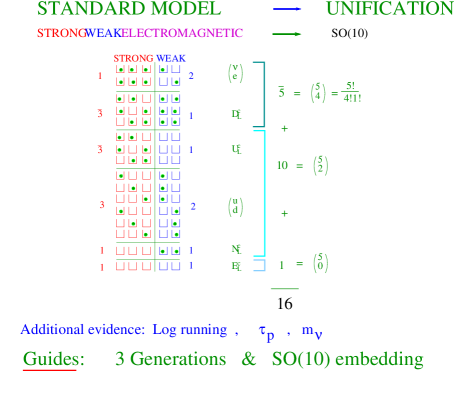
Figure 1: Embedding the Standard Model matter states in $SO(10)$ reduces the number of discrete parameters needed to account for the gauge charges from 54 to 1. This corroborates the assumption that grand unification structures play a role in nature. Additional evidence for this hypothesis is provided by: the logarithmic running of the Standard Model parameters; the longevity of the proton; the suppression of the left–handed neutrino masses.

The Standard Model provides compelling evidence for the realisation of GUT structures in nature. However, Grand Unified Theories still leave too many unexplained parameters, in particular in the flavour sector of the Standard Model. Further insight into the fundamental origin of these parameters can only be obtained in the mass scale beyond the GUT scale, i.e. the Planck scale, or in a theory of quantum gravity. String theory is a contemporary theory that while providing a perturbatively consistent approach to quantum gravity requires the existence of the gauge, matter and scalar states that are the basic building blocks of the Standard Model. String theory therefore provides the tools to develop a phenomenological approach to quantum gravity. Three generation quasi–realistic models that possess the $SO(10)$ embedding of the Standard Model matter states were constructed in the free fermionic formulation of the heterotic–string in four dimensions. These models provide a laboratory to explore how the parameters of the Standard Model are determined in a theory of quantum gravity. Many of the issues pertaining to the phenomenology of the Standard Model and grand unification have been studied in the context of these models. Among them: $\underline{\hbox{Top quark mass prediction}}$, which was predicted at a mass scale of $O(175-180)$GeV [3], several years prior to its experimental observation [4]; textures of the Standard Model quark and charged leptons mass and mixing matrices [5], as well as left–handed neutrino masses [6]; string gauge coupling unification [7]; proton stability [8]; squark degeneracy [9]; and moduli fixing [10]. Furthermore, the free fermionic construction produced the first examples of string models that give rise solely to the spectrum of the Minimal Supersymmetric Standard Model in the low energy effective field theory of the Standard Model charged sector. Such models are dubbed Minimal Standard Heterotic String Models [11].

The free fermionic models are $Z_{2}\times Z_{2}$ toroidal orbifolds at enhanced symmetry points in the toroidal moduli space [12]. As such they are related to other phenomenological studies of $Z_{2}\times Z_{2}$ orbifolds using other formalism, among those e.g. [13], and are similarly related to $Z_{2}$ orbifolds of $K_{3}\times T_{2}$ manifolds. Sitting at enhanced symmetry points in the moduli space, they exhibit rich symmetry structure that is being investigated from more mathematical point of views, e.g. [14]. How this rich symmetry structure plays a role in the phenomenological properties of the models remains to be determined, and some novel suggestions have been articulated [15, 16]. Among them the suggestion that self–duality under $T$–duality in string theory play a role in the vacuum selection [15], and the role of self–duality under spinor–vector duality [17] in light extra $U(1)$ symmetries and light sterile neutrinos [16]. Furthermore, the fact that the free fermionic models are constructed at an enhanced symmetry point in the toroidal moduli space, and the fact that the $Z_{2}\times Z_{2}$ orbifold can act on each of the six internal dimensions separately, enables the projection of all the internal geometrical moduli [10].

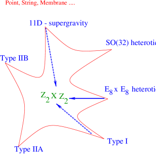
Figure 2: Perturbative treatment of elementary particles characterises them as idealised points, strings or membranes, … The non–perturbative dualities of supersymmetric string theories in ten dimensions, as well as 11 dimensional supergravity suggests probing the properties of different classes of string compactifications in the different limits.

While these properties suggest qualitative arguments how the true string vacuum may possess some of the characteristics exhibited by the phenomenological free fermionic models, it is important to explore and extract the properties of other classes of phenomenological string vacua [18]. Moreover, the different supersymmetric string theories in ten dimensions, as well as eleven dimensional supergravity, are mere limits of a more fundamental theory, typically dubbed $M$–theory. How should we then view the phenomenological studies of string vacua in any of these limits? The answer is that we should view each of these limits as providing an effective perturbative tool that enables us to probe some of the properties of the true $M$–theory vacuum, but not to fully characterise it. From this perspective, if the properties that we would like to capture are the existence of three generations and their embedding in $SO(10)$ multiplets then the effective limit that we should use is that of the $E_{8}\times E_{8}$ heterotic–string, as it is the only limit that produces chiral spinorial 16 representation of $SO(10)$ in the perturbative spectrum. On the other hand, dilaton stabilisation cannot be generated in the perturbative heterotic–string and requires moving away from this limit. It is therefore vital to explore the different classes of string compactifications in the different perturbative limits. This notion is depicted qualitatively in figure 2.

While spacetime supersymmetry is an appealing mathematical construction that provides a simpler framework to study the string vacua, there is so far no direct experimental evidence for its realisation in nature. Spacetime supersymmetry guarantees the absence of tachyonic modes in the physical spectrum, and ensures that these vacua are stable. In addition to the supersymmetric ten dimensional vacua, string theory produces several non–supersymmetric ten dimensional models. In lower dimensions all the non–supersymmetric vacua are connected to points in the moduli space that produce tachyons, and are therefore, in general, not expected to be stable. The issue of stability in non–supersymmetric string configurations occupies much of the literature in contemporary string phenomenology. In the spirit exhibited in figure 2 it is important to explore what can be learned by studying phenomenological models on compactifications of the non–supersymmetric ten dimensional string vacua, that have been classified in [19, 20, 21]. In general, the tachyonic states can be projected from the physical spectrum by GSO projections, other than by the one induced by the spacetime supersymmetry generator. We expect that generic vacua are connected to points in the moduli space that give rise to physical tachyons. The heterotic–string models in the free fermionic formulation produced a fertile space of three generation models with different $SO(10)$ subgroups and viable Higgs spectrum to produce quasi–realistic fermion masses. By that they provide a laboratory that can be employed to investigate compactifications of the non–supersymmetric ten dimensional string theories.

In the fermionic construction of the four dimensional heterotic–string all the additional degrees of freedom needed to cancel the conformal anomaly are represented in terms of free fermions propagating on the string worldsheet [23]. In the common notation the 64 worldsheet fermions in the lightcone gauge are denoted by:

   ${\underline{{\hbox{Left-Movers}}}}$:    $\psi^{\mu}_{1,2},~{}~{}~{}~{}{\chi_{i}},~{}~{}~{}~{}{y_{i},~{}~{}\omega_{i}}$    ${(i=1,\cdots,6)}$

   ${\underline{{\hbox{Right-Movers}}}}$:

$$~{}~{}~{}{\bar{\phi}}_{A=1,\cdots,44}~{}~{}=~{}~{}\begin{cases}~{}~{}{{\bar{y}}_{i}~{},~{}{\bar{\omega}}_{i}}&~{}~{}~{}{i=1,{\cdots},6}\cr&$ $\cr~{}~{}{{\bar{\eta}}_{i}}&~{}~{}~{}{U(1)_{i}~{}~{}~{}i=1,2,3{}{}}\cr~{}~{}{{\bar{\psi}}_{1,\cdots,5}}&~{}~{}~{}SO(10)$ $\cr~{}~{}{{\bar{\phi}}_{1,\cdots,8}}&~{}~{}~{}{SO(16)}$ $\end{cases}$$

where the six compactified internal coordinates correspond to $\{y,\omega|{\bar{y}},{\bar{\omega}}\}^{1,\cdots,6}$ and the gauge symmetries generated by sixteen complexified right–moving fermions are indicated. String models in the free fermionic formulation are constructed in terms of a set of boundary condition basis vectors and the Generalised GSO (GGSO) projection coefficients of the one loop partition function [23]. The free fermion models correspond to $Z_{2}\times Z_{2}$ orbifolds with discrete Wilson lines [12].

2 Realistic free fermionic models – old school

Free fermionic heterotic–string models with three generations were built since the late eighties [11, 24, 25, 26]. The early models consisted of highlighted examples that shared an underlying GUT structure The basis vectors spanning the different models contained the common set of five NAHE–set vectors [27], denoted as $\{{\bf 1},S,b_{1},b_{2},b_{3}\}$. The gauge group at the level of the NAHE–set is $SO(10)\times SO(6)^{3}\times E_{8}$, with forty–eight multiplets in the spinorial 16 representation of $SO(10)$, obtained from the twisted sectors of the $Z_{2}\times Z_{2}$ orbifold $b_{1}$, $b_{2}$ and $b_{3}$. The $S$–vector generates $N=4$ spacetime supersymmetry, which is reduced to $N=2$ by the basis vector $b_{1}$ and to $N=1$ by the inclusion of both $b_{1}$ and $b_{2}$. The GSO projection induced by $b_{3}$ either preserves or removes the remaining supersymmetry. The second stage in the old school free fermionic heterotic–string model building consists of adding to the NAHE–set three additional basis vectors, typically denoted as $\{\alpha,\beta,\gamma\}$. The additional basis vectors break the $SO(10)$ gauge symmetry to one of its subgroups and at the same time reduce the number of generations to three. In the standard–like models of [11] the $SO(10)$ gauge symmetry is reduced to $SU(3)\times SU(2)\times U(1)_{B-L}\times U(1)_{R}$, and the weak hypercharge is given by the combination

$$U(1)_{Y}={1\over 2}(B-L)+T_{3_{R}}\in SO(10).$$

Each of the $b_{1}$, $b_{2}$ and $b_{3}$ sectors produces one generation that form complete 16 multiplets of $SO(10)$. The models admit the needed scalar states to further reduce the gauge symmetry and to produce a viable fermion mass and mixing spectrum [4, 5, 6].

3 Classification of fermionic $Z_{2}\times Z_{2}$ orbifolds – modern school

Systematic classification of fermionic $Z_{2}\times Z_{2}$ heterotic–string orbifolds has been pursued since 2003. The classification of vacua with unbroken $SO(10)$ gauge group was performed in [28] and extended to vacua with: $SO(6)\times SO(4)$ subgroup in [29]; $SU(5)\times U(1)$ subgroup in [30]; $SU(3)\times SU(2)\times U(1)^{2}$ subgroup in [31]; $SU(3)\times U(1)\times SU(2)^{2}$ subgroup in [32, 33]. In the free fermionic classification method the string models are produced by a fixed set of boundary condition basis vectors, consisting of between twelve to fourteen basis vectors, $B=\{v_{1},v_{2},\dots,v_{14}\}.$ The vacua with unbroken $SO(10)$ group are produced by a set of twelve basis vectors

$$v_{1}={\bf 1} = \{\psi^{\mu},\ \chi^{1,\dots,6},y^{1,\dots,6},\omega^{1,\dots,6}~{}~{}~{}|~{}~{}~{}\bar{y}^{1,\dots,6},\bar{\omega}^{1,\dots,6},\bar{\eta}^{1,2,3},\bar{\psi}^{1,\dots,5},\bar{\phi}^{1,\dots,8}\},$$

$$v_{2}=S = \{\psi^{\mu},\chi^{1,\dots,6}\},$$

$$v_{3}=z_{1} = \{\bar{\phi}^{1,\dots,4}\},$$

$$v_{4}=z_{2} = \{\bar{\phi}^{5,\dots,8}\},$$ (1)

$$v_{4+i}=e_{i} = \{y^{i},\omega^{i}|\bar{y}^{i},\bar{\omega}^{i}\},\ i=1,\dots,6,~{}~{}~{}~{}~{}~{}~{}~{}~{}~{}~{}~{}~{}~{}~{}~{}~{}~{}~{}~{}~{}N=4~{}~{}{\rm Vacua}$$

$$v_{11}=b_{1} = \{\chi^{34},\chi^{56},y^{34},y^{56}|\bar{y}^{34},\bar{y}^{56},\bar{\eta}^{1},\bar{\psi}^{1,\dots,5}\},~{}~{}~{}~{}~{}~{}~{}~{}N=4\rightarrow N=2$$

$$v_{12}=b_{2} = \{\chi^{12},\chi^{56},y^{12},y^{56}|\bar{y}^{12},\bar{y}^{56},\bar{\eta}^{2},\bar{\psi}^{1,\dots,5}\},~{}~{}~{}~{}~{}~{}~{}~{}N=2\rightarrow N=1.$$

The first ten vectors preserve $N=4$ spacetime supersymmetry and the last two are the $Z_{2}\times Z_{2}$ orbifold twists. The third twisted sector of the $Z_{2}\times Z_{2}$ orbifold is obtained as the combination $b_{3}=b_{1}+b_{2}+x$, where the $x$–sector is obtained from the combination

$$x={\bf 1}+S+\sum_{i=1}^{6}e_{i}+\sum_{k=1}^{2}z_{k}=\{{\bar{\psi}}^{1,\cdots,5},{\bar{\eta}}^{1,2,3}\}.$$ (2)

The reduction of the $SO(10)$ symmetry to the $SO(6)\times SO(4)$ subgroup is achieved by including in the basis the vector [29]

$$v_{13}=\alpha=\{\bar{\psi}^{4,5},\bar{\phi}^{1,2}\},$$ (3)

whereas the reduction to the $SU(5)\times U(1)$ subgroup is achieved with the basis vector [30]

$$v_{13}=\alpha=\{\overline{\psi}^{1,\dots,5}=\textstyle\frac{1}{2},\overline{\eta}^{1,2,3}=\textstyle\frac{1}{2},\overline{\phi}^{1,2}=\textstyle\frac{1}{2},\overline{\phi}^{3,4}=\textstyle\frac{1}{2},\overline{\phi}^{5}=1,\overline{\phi}^{6,7}=0,\overline{\phi}^{8}=0\,\},$$ (4)

and the reduction to the $SU(3)\times SU(2)\times U(1)^{2}$ is produced by adding the vectors in (3) and (4) as two separate vectors, $v_{13}$ and $v_{14}$ to the basis [31]. The reduction of the $SO(10)$ gauge group to the Left–Right Symmetric (LRS) subgroup is obtained with the basis vector

$$v_{13}=\alpha=\{\overline{\psi}^{1,2,3}=\frac{1}{2}\;,\;\overline{\eta}^{1,2,3}=\frac{1}{2}\;,\;\overline{\phi}^{1,\ldots,6}=\frac{1}{2}\;,\;\overline{\phi}^{7}\}.$$ (5)

For a fixed set of basis vectors, the free fermionic models are spanned by varying the independent GGSO projection coefficients. For instance, in the $SO(6)\times SO(4)$ models 66 phases are independent, and the remaining phases are determined by imposing modular invariance, and $N=1$ spacetime supersymmetry. Varying the GGSO phases randomly spans a space of approximately $10^{19.9}$ $Z_{2}\times Z_{2}$ orbifold models. A specific choice of the 66 discrete phases corresponds to a distinct string vacuum with massless and massive physical spectrum. The analysis proceeds by applying systematic tools to analyse the entire massless spectrum.

The free fermionic classification method provides powerful tools to analyse large classes of string models and extract properties of the entire space of vacua. Furthermore, models with specific phenomenological properties can be fished out and their charges and couplings analysed in greater detail. The free fermionic classification methodology led to several seminal results. The first, depicted in figure 3, is the discovery of Spinor–Vector Duality (SVD) under the exchange of the total number of $({\bf 16}+\overline{\bf 16})$ spinorial and 10 vectorial representations of $SO(10)$ [17]. The SVD arises from the breaking of the (2,2) worldsheet supersymmetry to (2,0), and is a general property of heterotic–string vacua. From a worldsheet perspective, the SVD suggests that all string vacua are connected by interpolations or by orbifolds, but are distinct in the low energy effective field theory [34].

Figure 3: Density plot showing the spinor–vector duality in the space of $Z_{2}\times Z_{2}$ heterotic–string models. The plot shows the number of vacua with a given number of $({\bf 16}+\overline{\bf 16})$ and 10 multiplets of $SO(10)$ and is invariant under exchange of rows and columns, reflecting the spinor–vector duality underlying the entire space of vacua.

Another important result from the free fermionic classification approach is the discovery of exophobic string vacua [29]. Heterotic–string vacua with broken $SO(10)$ GUT symmetry, and that maintain the $SO(10)$ embedding of the weak hypercharge, necessarily contain fractionally charged states in their spectrum, which may be confined to the massive spectrum. Such models are dubbed as exophobic string models. As illustrated in figures 5 and 5, three generation exophobic string vacua were found in the space of fermionic $Z_{2}\times Z_{2}$ orbifolds with $SO(6)\times SO(4)$ gauge symmetry but not with $SU(5)\times U(1)$. The two figures illustrate the utility of the free fermion classification machinery in extracting definite properties of the entire space of scanned vacua.

Figure 4: Number of 3–generation models versus total number of exotic states in $SO(6)\times SO(4)$ vacua.

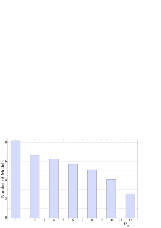
Figure 5: Number of exophobic models versus number of generations in $SU(5)\times U(1)$ string models.

	Constraints	Total models in sample	Probability
	No Constraints	$1000000000$	$1$
(1)	+ No Enhancements	$708830165$	$7.09\times 10^{-1}$
(2)	+ Complete Families	$70241057$	$7.02\times 10^{-2}$
(3)	+ No Chiral Exotics	$43660665$	$4.37\times 10^{-2}$
(4)	+ Three Generations	$1486$	$1.49\times 10^{-6}$
(5)	+ SM Light Higgs	$1$	$1.00\times 10^{-9}$
	+ & Heavy Higgs

Table 1: Statistics for the LRS models derived using fully randomised method.

	Constraints	Total models in sample	Probability
	No Constraints	9919488	$1$
(1)	+ No Observable Enhancements	8894808	$0.9$
(2)	+ No Chiral Exotics	1699104	$0.17$
(3)	+ Complete Generations	1698818	$0.17$
(4)	+ Three Generations	827333	$8.3\times 10^{-2}$
(5)	+ SM Light Higgs	732728	$7.4\times 10^{-2}$
	& Heavy Higgs

Table 2: Statistics for the LRS models derived from fertile cores

The free fermionic random classification methodology reaches its utility limit in the classification of SLM [31] and LRS models [32, 33]. In both cases the models contain two vectors that break the $SO(10)$ GUT symmetry. Resulting in the proliferation of exotic states producing sectors. The frequency of viable models is then substantially reduced compared to the PS and FSU5 models. The computation time required for extracting substantial number of phenomenologically viable models becomes excessive, rendering the approach unpractical. Adaptation of the methodology is warranted. This is achieved by dividing the process in two stages. The first consist of generating random sets of GGSO phases at the $SO(10)$ level, i.e. GGSO phases that do not involve the basis vectors that break the $SO(10)$ GUT symmetry, subject to certain fertility conditions. These conditions guarantee that the full models admit some basic phenomenological characteristics, like the existence of three generations, or the existence of electroweak Higgs doublets. The random process at the $SO(10)$ level produces fertile cores that are guaranteed to produce the phenomenological characteristics that are set a priori. Around each of these fertile cores a complete classification of the $SO(10)$ breaking phases is then performed. In this manner a space of $10^{7}$ three generation Standard–like Models with the standard light and heavy Higgs states was produced [31]. Tables 1 and 2 present a comparison of the methods in the case of the LRS models [32, 33]. It is evident from the two tables that the fertile core method [33] facilitates the extraction of phenomenologically viable models when the total space of models becomes exceedingly large. On the other hand, it allows the analysis of general properties of the space of vacua, which is not the case in the genetic algorithm method [35]. The stage is now ripe for the application of novel computational methods for the identification of the fertility conditions [36].

4 Tachyonic ten dimensional vacua

The free fermionic formalism provides the tools to classify and analyse large classes of $Z_{2}\times Z_{2}$ toroidal orbifold compactifications. We can use this formalism to construct phenomenological models that correspond to compactifications of the ten dimensional tachyonic vacua. A good starting point for our discussion is the $E_{8}\times E_{8}$ heterotic–string in ten dimensions, whose partition function is given by,

$$Z^{+}_{10d}=\frac{1}{{\tau_{2}}^{4}{(\eta\overline{\eta})}^{8}}({V}_{8}-{S}_{8})\left(\overline{O}_{16}+\overline{S}_{16}\right)\left(\overline{O}_{16}+\overline{S}_{16}\right),$$ (6)

and the level–one $SO(2n)$ characters are given by,

$$~{}~{}~{}O_{2n} = {\textstyle{1\over 2}}\left({\theta_{3}^{n}\over\eta^{n}}+{\theta_{4}^{n}\over\eta^{n}}\right)\,~{}~{}~{}~{}~{}~{}~{},~{}~{}~{}~{}~{}~{}~{}~{}V_{2n}={\textstyle{1\over 2}}\left({\theta_{3}^{n}\over\eta^{n}}-{\theta_{4}^{n}\over\eta^{n}}\right)\,,$$

$$S_{2n} = {\textstyle{1\over 2}}\left({\theta_{2}^{n}\over\eta^{n}}+i^{-n}{\theta_{1}^{n}\over\eta^{n}}\right)\,~{}~{}~{},~{}~{}~{}~{}~{}~{}~{}C_{2n}={\textstyle{1\over 2}}\left({\theta_{2}^{n}\over\eta^{n}}-i^{-n}{\theta_{1}^{n}\over\eta^{n}}\right)\,.$$

The ten dimensional $SO(16)\times SO(16)$ heterotic–string is obtained by applying the orbifold projection

$$g=(-1)^{F+F_{z_{1}}+F_{z_{2}}}$$ (7)

where $F$ is the spacetime fermion number, taking $S_{8}\rightarrow-S_{8}$ and $F_{z_{1},z_{2}}$ are the fermion numbers of the two $E_{8}$ factors, taking $S_{16}^{1,2}\rightarrow-S_{16}^{1,2}$. The partition function of the $SO(16)\times SO(16)$ heterotic–string is given by

$$Z_{10d}^{-}~{}=~{} \left[\right. V_{8}\left(\overline{O}_{16}\overline{O}_{16}+\overline{S}_{16}\overline{S}_{16}\right)~{}~{}-~{}S_{8}\left(\overline{O}_{16}\overline{S}_{16}+\overline{S}_{16}\overline{O}_{16}\right)$$ (8)

$$+ O_{8}\left(\overline{C}_{16}\overline{V}_{16}+\overline{V}_{16}\overline{C}_{16}\right)~{}-\left.~{}C_{8}\left(\overline{C}_{16}\overline{C}_{16}+\overline{V}_{16}\overline{V}_{16}\right)\right]\,,$$ (9)

where I omitted the prefactor due to the uncompactified dimensions. From the partition function in eq. (9) it is observed that the would–be tachyonic term, $O_{8}\left(\overline{C}_{16}\overline{V}_{16}+\overline{V}_{16}\overline{C}_{16}\right)$ generates only massive physical states. Upon compactifications to lower dimensions, tachyonic states will, in general, appear in the spectrum, but can be projected out in special cases. A priori, we can consider the ten dimensional tachyonic vacua and similarly project out the tachyons from the spectrum in special cases.

In the free fermion formulation, the $E_{8}\times E_{8}$ and $SO(16)\times SO(16)$ models are specified in terms of a common set of basis vectors

$$v_{1}={\bf 1} = \{\psi^{\mu},\ \chi^{1,\dots,6}|\overline{\eta}^{1,2,3},\overline{\psi}^{1,\dots,5},\overline{\phi}^{1,\dots,8}\},$$

$$v_{2}=z_{1} = \{\overline{\psi}^{1,\dots,5},\overline{\eta}^{1,2,3}\},$$

$$v_{3}=z_{2} = \{\overline{\phi}^{1,\dots,8}\}.$$ (10)

The spacetime supersymmetry generator is given by the combination

$$S={\bf 1}+z_{1}+z_{2}=\{{\psi^{\mu}},\chi^{1,\dots,6}\}.$$ (11)

The GGSO phase $C{z_{1}\atopwithdelims[ ]z_{2}}=\pm 1$ then selects between the $E_{8}\times E_{8}$ or $SO(16)\times SO(16)$ heterotic–string models in ten dimensions. The relation in eq. (11) implies that in ten dimensions the reduction pattern $E_{8}\times E_{8}\rightarrow SO(16)\times SO(16)$ is correlated with the reduction of spacetime supersymmetry. Eq. (11) does not hold in lower dimensions. Compactifications of the $SO(16)\times SO(16)$ heterotic–string model to four dimensions form the basis for the phenomenological studies of non–supersymmetric heterotic–string vacua.

To produce the ten dimensional tachyonic vacua we can start with the $E_{8}\times E_{8}$ partition function and apply the orbifold

$$g=(-1)^{F+F_{z_{1}}}\,.$$ (12)

The resulting partition function, given by

$$\left(V_{8}\overline{O}_{16}-S_{8}\overline{S}_{16}+O_{8}\overline{V}_{16}-C_{8}\overline{C}_{16}\right)\left(\overline{O}_{16}+\overline{S}_{16}\right),$$ (13)

is the partition function of the $SO(16)\times E_{8}$ non–supersymmetric and tachyonic heterotic–string vacuum. It is seen that the term $O_{8}\overline{V}_{16}\overline{O}_{16}$ in the partition function generates a tachyonic state in the vectorial $16$ representation of $SO(16)$. The non-supersymmetric tachyonic string vacua in ten dimensions were classified in refs. [19, 21].

The $SO(16)\times E_{8}$ vacuum is produced in the fermionic language by the basis vectors $\{{\bf 1},z_{1}\}$ from eq. (10), irrespective of the choices of the GGSO phases [34]. The tachyon in this model is obtained by acting on the right–moving vacuum with a single fermionic oscillator:

$$|~{}0\rangle_{L}\otimes{\bar{\phi}}^{a}|0\rangle_{R}\,,$$ (14)

where in ten dimensions $a=1,\cdots,32$. In both the supersymmetric $E_{8}\times E_{8}$ and non–supersymmetric $SO(16)\times SO(16)$ vacua, the tachyonic states in eq. (14) are projected out by the GSO projection induced by the $S$–vector, which is the spacetime supersymmetry generator. Other ten dimensional vacua are similarly generated by replacing the $z_{1}$ basis vectors with $z_{1}=\{{\bar{\phi}}^{1,\cdots,4}\}$ and additional $z_{i}$ basis vectors with four periodic worldsheet fermionic and utmost two overlapping periodic fermions. All these vacua are in principle connected by interpolations or orbifolds along the lines of ref. [20, 22], and, in general, will contain tachyons in their spectrum. Our interest here is rather in the possibility of constructing tachyon free phenomenological vacua, starting from the tachyonic ten dimensional vacua. The lesson to draw from the ten dimensional exercise is that these models can be constructed by removing the ten dimensional vector $S={\bf 1}+z_{1}+z_{2}$ from the basis of the phenomenological four dimensional models. An alternative to the removal of the $S$–vector from the basis is to augment it with periodic right–moving fermions. A convenient choice is given by

$${\tilde{S}}=\{\psi^{1,2},\chi^{1,2},\chi^{3,4},\chi^{5,6}|{\bar{\phi}}^{1,\cdots,~{}4}\}\equiv~{}1~{}.$$ (15)

In this case the spectrum does not contain massless gravitinos, and the untwisted tachyonic states

$$|0\rangle_{L}\otimes{\bar{\phi}}^{1,\cdots,~{}4}|0\rangle_{R}$$ (16)

are invariant under the ${\tilde{S}}$–vector projection. These are the tachyonic states that descend from the ten dimensional vacuum. The advantage of using the ${\tilde{S}}$–vector is that its projection on the chiral generations is retained, hence facilitating the construction of three generation models. Our aim is to construct a phenomenological tachyon free three generation model that can be interpreted as compactification of a tachyonic ten dimensional vacuum, where the ten dimensional tachyonic modes can be projected out by additional GSO projections, rather than by the $S$–vector projection. Furthermore, we would like our model to sit at a fixed point in the moduli space, which will prevent it from being interpolated to a point where tachyonic modes are generated. This can be achieved by projecting out the moduli fields from the string model.

5 A tachyon free Standard–like Model

Our tachyon free three generation Standard–like model is obtained by using a modified NAHE–set [37], with the $S$–vector replaced by the $\tilde{S}$–vector, and is referred to as the ${\overline{\rm NAHE}}$–set. In this case the untwisted tachyonic states in (16) are projected out by the projection of each of the basis vectors $b_{i}$ $i=1,2,3$. The three basis vectors that extend the ${\overline{\rm NAHE}}$–set are given by

(21)

(26)

that together with a specific choice of one–loop GGSO projection coefficients produce a tachyon free three generation Standard–like Model [37]. As a consequence of the substitution $S\rightarrow{\tilde{S}}$, the resulting spectrum possesses some novel features. First, I remark that the basis vectors defined by the NAHE–set, together with those in eq. (26), are identical to those used in ref. [38]. The basis vectors and GGSO phases that generate the non–supersymmetric model in ref. [37] are identical to those used in ref. [38], up to the substitution $S\rightarrow{\tilde{S}}$, and the corresponding adjustment of the GGSO phases. The two models therefore share some features. In particular with the respect to the untwisted spectrum and the moduli space, as the states from the untwisted sector and the corresponding moduli, only depend on the basis vectors and the corresponding spin–statistics phases. Similarly, the three chiral generations from the sectors $b_{1}$, $b_{2}$ and $b_{3}$ that produce the Standard Model spectrum and their charges under the four dimensional gauge group are the same as those of ref. [38]. On the other hand the supersymmetric spectrum in the two models differs substantially, and also with respect to the non–supersymmetric model that can be obtained from the model of ref. [38] by projecting out the $N=1$ spacetime supersymmetry generator by a GGSO projection. Basically, the substitution $S\rightarrow{\tilde{S}}$ keeps the states from the sectors $b_{i}$ $i=1,2,3$ massless, whereas the states from the sectors ${\tilde{S}}+b_{i}$ are massive. In models in which supersymmetry is broken by a GGSO phase [39], the states from the sectors $S+b_{i}$ are retained, though their charges may be modified from those in the $b_{i}$ sectors. In these models the chiral spectrum retains its underlying supersymmetric structure. This is a notable distinction between the two classes of compactifications, with important phenomenological consequences. In particular, it is relevant for the question of the role of spacetime supersymmetry in string derived GUT models, and how vital it is for the viability of the models. Supersymmetry has played an important role in maintaining computational stability between the electroweak and GUT scales, but whether it is a necessary ingredient is yet to be determined.

5.1 moduli fixing

As discussed above all the ten dimensional vacua can be connected by interpolations in a compactified dimension [20, 22], and the same is expected in the four dimensional models [40]. In that case the non–supersymmetric models are expected to be connected to points in the moduli space that are tachyonic. Hence, in general, these vacua are not expected to be stable. However, there may be exceptions to the general expectation. The free fermionic models are $Z_{2}\times Z_{2}$ orbifolds at enhanced symmetry points in the moduli space. This basic characteristic of these vacua mean that we can mod them out by more symmetries and that we can treat the internal dimensions as six real circles rather than as three complex tori. Furthermore, the enhanced symmetry point is realised with a non–trivial anti–symmetric $B$ field, which entails that the internal spaces realised in the models are not standard geometrical spaces. To investigate the moduli spaces in these constructions is instrumental to study the model generated by extending the NAHE–set with the basis vector $z_{1}=\{{{\bar{\psi}}^{1,\cdots,5},{{\bar{\eta}}^{1},{\bar{\eta}}^{2},{\bar{\eta}}^{3}}}\}=1$, which can be generated by the set $\{1,S,z_{1},z_{2},b_{1},b_{2}\}$, with $z_{2}=\{{\bar{\phi}}^{1,\cdots,8}\}$. The same model is reproduced as a $Z_{2}\times Z_{2}$ orbifold of an $SO(12)$ Narain lattice, which is obtained by setting the moduli at the self-dual point, with the metric given by the Cartan matrix of $SO(12)$ and the anti–symmetric tensor field as $b_{ij}=g_{ij}$ $i>j$. Setting the phase $C{z_{1}\atopwithdelims[ ]z_{2}}=+1$ produces a model with $SO(4)^{3}\times E_{6}\times U(1)^{2}\times E_{8}$ gauge symmetry and 24 generations in the chiral 27 representation of $E_{6}$, eight from each of the sectors $b_{1}$, $b_{2}$ and $b_{3}$. Three additional $27\oplus{\overline{27}}$ representations are obtained from the untwisted sector. The 27 representation decomposes as $27\rightarrow 16_{1/2}+10_{-1}+1_{2}$ under $E_{6}\rightarrow SO(10)\times U(1)$, where the $16$ multiplets are obtained from the sectors $b_{j}$ and the $10+1$ are obtained from the sectors $b_{j}+z_{1}$. In addition to the $10+1$ states the sectors $b_{j}+z_{1}$ produce 24 $E_{6}$ singlets that are identified as the twisted moduli, In the realistic free fermionic models the phase $C{z_{1}\atopwithdelims[ ]z_{2}}=-1$ is set. In this case the $E_{6}\times U(1)^{2}\times E_{8}$ symmetry is reduced to $SO(10)^{3}\times U(1)^{3}\times SO(16)$, and the states from the sectors $b_{j}+z_{1}$ are mapped to vectorial 16 representations of the hidden $SO(16)$ gauge group. Hence, the twisted moduli are projected out.

The untwisted moduli are given in the fermionic constructions in terms of worldsheet Thirring interactions of the form [10]

$$(R-{1\over R})J_{L}^{i}(z){\bar{J}}_{R}^{j}({\bar{z}})=(R-{1\over R})y^{i}\omega^{i}{\bar{y}}^{j}{\bar{\omega}}^{j}.$$ (27)

Thus, at the self–dual point, $R=1/R$ the worldsheet Thirring interactions vanish and the fermions are free. However, the moduli correspond to massless fields in the string spectrum and are not fixed. To identify them we need to look at terms of the form of eq. (27) that are invariant under the transformation properties defined the boundary condition basis vectors. In the case of symmetric $Z_{2}\times Z_{2}$ orbifolds the Thirring interactions that remain invariant are

$$J_{L}^{1,2}{\bar{J}}_{R}^{1,2}~{}~{}~{}~{}~{}~{}~{}~{};~{}~{}~{}~{}~{}~{}~{}~{}J_{L}^{3,4}{\bar{J}}_{R}^{3,4}~{}~{}~{}~{}~{}~{}~{}~{};~{}~{}~{}~{}~{}~{}~{}~{}J_{L}^{5,6}{\bar{J}}_{R}^{5,6}$$

$y^{1,2}\omega^{1,2}{\bar{y}}^{1,2}{\bar{\omega}}^{1,2}~{}~{}~{}~{}~{};~{}~{}~{}~{}~{}y^{3,4}\omega^{3,4}{\bar{y}}^{3,4}{\bar{\omega}}^{3,4}~{}~{}~{};~{}~{}~{}y^{5,6}\omega^{5,6}{\bar{y}}^{5,6}{\bar{\omega}}^{5,6}$,

corresponding to three Kähler and three complex structure moduli. These set of untwisted moduli are always present in symmetric $Z_{2}\times Z_{2}$ orbifold and correspond to a set of untwisted fields in these string models. The free fermion systematic method has thus far been developed solely for models with symmetric boundary conditions. Hence, all these models contain the $Z_{2}\times Z_{2}$ moduli fields that are not fixed. On the other hand, the “old school” NAHE–based models utilise both symmetric and asymmetric boundary conditions. The effect of using asymmetric boundary conditions results in the projection of untwisted moduli, with the possibility of projecting out all of internal geometrical moduli [10]. The possibility of projecting out all of the internal geometrical moduli depends on the assignment of boundary conditions for the set of internal worldsheet fermions $\{y,\omega|{\bar{y}},{\bar{\omega}}\}^{1,\cdots,6}$. In order to project all the internal geometrical moduli, it is crucial that it corresponds to separate asymmetric action on each of the $S^{1}$ circles of the six dimensional internal torus [10]. An example of a model that realises this asymmetric assignment is the model in eq. (26). Consequently, all the internal moduli in this model are fixed.

In supersymmetric vacua there may still exist moduli that correspond to flat directions of the scalar potential. However, it was argued in ref. [38] that in the model defined by eq. (26) there are no supersymmetric flat directions that are exact to all orders in the superpotential. To understand the origin of this claim we have to examine more carefully the boundary conditions in eq. (26). This model utilises both symmetric and asymmetric boundary conditions, with respect to the $b_{1}$ and $b_{2}$ twisted planes, in the two vectors $\alpha$ and $\beta$ that reduce the $SO(10)$ GUT symmetry to the Pati–Salam subgroup, which results in the projection of untwisted charged fields. It was therefore argued that this is an example of a model in which all the moduli, aside from the dilaton, are fixed perturbatively, whereas the dilaton may be fixed by hidden sector non–perturbative effects. In both cases it implies that supersymmetry is broken and the vacuum is frozen. In the ${\overline{\rm NAHE}}$–based model supersymmetry is broken at tree level by the spectrum, and a non–vanishing cosmological constant is generated at one–loop, whereas in the NAHE–based model, supersymmetry is broken at one–loop by the non–vanishing Fayet–Iliopoulos term, and a non–vanishing cosmological constant is generated at two–loops.

6 The EPOQM and the closed universe

The synthesis of quantum mechanics and gravity is the prevailing enigma of theoretical physics on the fundamental frontier. The main contemporary effort entails the quantisation of general relativity and spacetime, e.g. in the framework of string theory. The main successes of string theory are that while it provides a viable perturbative approach to quantum gravity, it unifies the gauge, gravitational and matter structures that form the bedrock of elementary particle physics. By doing that string theory provides the framework for the construction of phenomenologically realistic models, i.e. it provides a relevant framework to explore how the experimental parameters that are used to parameterise contemporary experimental observations, may be obtained in a perturbatively consistent theory of quantum gravity. The issue is not whether string theory is a “Theory of Everything”, which is an ill defined concept, but rather that string theory is the leading contemporary framework to explore the synthesis of the gauge and gravitational interactions. The state of the art in that respect is the construction of string models that reproduce the structure of the Minimal Supersymmetric Standard Model [11]. Nevertheless, string theory does not provide a satisfactory starting point for the formulation of quantum gravity from a fundamental axiomatic hypothesis á la general relativity or quantum mechanics. While general relativity emanates from the geometrical principles of equivalence and covariance, and quantum mechanics main tenet is the probability interpretation of the wave function, no such basic principle underlies string theory.

A plausible starting point for an axiomatic formulation of quantum gravity stems from a basic duality symmetry that underlies string theory and promoting it to the level of a fundamental principle. $T$–duality is a basic property of string theory. We may interpret $T$–duality on a circle as phase–space duality in compact space. A plausible assumption is then to take phase–space duality as a defining criteria of quantum gravity. We may start for that purpose with Hamilton’s equations of motion

$$\dot{q}={\partial{H}\over{\partial{p}}}~{}~{}~{}~{},~{}~{}~{}~{}\dot{p}=-{\partial{H}\over{\partial q}},~{}~{}~{}~{}~{}~{}~{}~{}~{}$$ (28)

which are invariant under the exchange $p\rightarrow-q$, that, in general breaks down once a potential function, $V(q)$, is specified. What we seek is a formalism with manifest phase–space duality. We may define the phase–space duality in the context of Legendre transformations, due to their involutive property. For that purpose we introduce a generating scalar function $p=\partial_{q}S(q)$ and a dual function $q=\partial_{p}T(p)$. The two functions are Legendre dual of each other, and each is associated with a second order differential equation. In this sense we obtain a formalism with manifest $p\leftrightarrow q$ and $S\leftrightarrow T$ duality with the dual set of equations [41]

$$~{}~{}~{}~{}~{}p~{} = ~{}{{\partial S_{0}}\over{\partial q}}~{}~{}~{}~{}~{}~{}~{}~{}~{}~{}~{}~{}~{}~{}~{}~{}~{}~{}~{}~{}~{}~{}~{}~{}~{}~{}~{}~{}~{}~{}~{}~{}~{}~{}~{}~{}~{}q~{}=~{}{{\partial T_{0}}\over{\partial p}}$$ (29)

$$~{}~{}~{}~{}~{}S_{0}~{} = ~{}p{{\partial T_{0}\over\partial p}}-T_{0}~{}~{}~{}~{}~{}~{}~{}~{}~{}~{}~{}~{}~{}~{}~{}~{}~{}~{}~{}~{}~{}~{}~{}~{}~{}~{}~{}T_{0}~{}=~{}q{{\partial S_{0}\over\partial q}}-S_{0}$$ (30)

$$\left({{\partial^{2}~{}~{}}\over\partial S_{0}^{2}}+{U(S_{0})}\right)\left({{q\sqrt{p}}\atop\sqrt{p}}\right)=0~{}~{}~{}~{}~{}~{}~{}~{}~{}~{}\left({{\partial^{2}~{}~{}}\over\partial T_{0}^{2}}+{\cal V}(T_{0})\right)\left({{p\sqrt{q}}\atop\sqrt{q}}\right)=0,$$ (31)

where, for simplicity, the stationary case is considered. There are two important points to note. The first is that the Legendre transformation is undefined for linear functions. Hence, Legendre duality restricts that the scalar function $S(q)$ satisfies

$$\frac{\partial^{2}S(q)}{\partial q^{2}}\neq 0~{}.$$ (32)

The second essential feature is the existence of self–dual states, with the property that $pq=\gamma=constant$, which are simultaneous solutions of the dual pictures. In these cases $S_{0}=-T_{0}+constant$, and

$$S_{0}(q)=\gamma\ln\gamma_{q}q~{}~{}~{}~{}~{}~{}~{}~{}~{}~{}~{}~{}~{}~{}~{}~{}~{}T_{0}(p)=\gamma\ln\gamma_{p}p$$

Hence, $S_{0}~{}+~{}T_{0}~{}=~{}pq~{}=~{}\gamma$, where $\gamma_{q}\gamma_{p}\gamma={\rm e}$ and $\gamma_{q}$, $\gamma_{p}$ are constants.

Classically, a solution of the Hamilton equations of motion is obtained by the Hamilton–Jacobi formalism, in which a transformation from a non–trivial Hamiltonian to a trivial Hamiltonian is induced by canonical transformations. A generating function is defined by the relation $p=\partial_{q}S(q)$, from the old phase space variables, $(q,p)$ to the new phase space variables $(Q,P)$, which are constants of the motion. The solution to this problem is given by the Classical Hamilton–Jacobi equation

$${1\over{2m}}\left({{\partial{S}_{0}}\over{\partial q}}\right)^{2}~{}~{}+~{}~{}V(q)~{}~{}-~{}~{}E~{}~{}\equiv~{}~{}{1\over{2m}}\left({{\partial{S}_{0}}\over{\partial q}}\right)^{2}~{}~{}+W(q)~{}~{}=~{}~{}0,$$ (33)

where the stationary case is discussed here for simplicity. The canonical transformations treat the phase space variables as independent variables and their functional dependence is extracted from the solution of the Hamilton–Jacobi equation via the relation $p=\partial_{q}S(q)$. Quantum mechanically the phase space variables are not independent, and we may therefore consider setting the problem in a reverse order. Namely, assume that a trivialising transformation always exists, but that the phase space variables are dependent in the application of the trivialising transformation. This led to the formulation of the Equivalence Postulate of Quantum Mechanics (EPOQM) [41], which posits that all physical systems that are labelled by a potential function $W(q)=V(q)-E$, can be connected by coordinate transformations. However, this cannot be implemented consistently in classical mechanics, due to the existence of the physical state $W(q)\equiv 0$, which is a fixed point under the transformations $q\rightarrow{\tilde{q}}(q)$. Considering the CSHJE in this case, it is seen that the solution is $S_{0}=Aq+B$, with constants $A$ and $B$. The equivalence postulate implies that the HJ equation is covariant under coordinate transformations. Consistent implementation of the EPOQM necessitates modification of the HJ equation by adding to it a yet to be defined function $Q(q)$. The modified HJ equation takes the form

$$~{}{1\over{2m}}\left({{\partial{S}_{0}}\over{\partial q}}\right)^{2}~{}~{}+~{}~{}W(q)~{}~{}+~{}~{}Q(q)~{}~{}=~{}~{}0.$$ (34)

Under the transformations $q\rightarrow{\tilde{q}}(q)$ the functions $W(q)$ and $Q(q)$ transform as

$${\tilde{W}}({\tilde{q}}) = \left({{\partial{\tilde{q}}}\over{\partial q}}\right)^{-2}W(q)+({\tilde{q}};q),$$

$${\tilde{Q}}({\tilde{q}}) = \left({{\partial{\tilde{q}}}\over{\partial q}}\right)^{-2}Q(q)-({\tilde{q}};q),$$

with ${\tilde{S}}_{0}({\tilde{q}})~{}=~{}S_{0}(q)$. The functions $W(q)$ and $Q(q)$ transform as quadratic differentials, up to an additive term, and the combination $(W(q)+Q(q))$ transforms as a quadratic differential. Considering the transformations $q^{a}\rightarrow q^{b}\rightarrow q^{c}$ and $q^{a}\rightarrow q^{c}$ and the induced transformations $W^{a}(q^{a})\rightarrow W^{b}(q^{b})\rightarrow W^{c}(q^{c})$ and $W^{a}(q^{a})\rightarrow W^{c}(q^{c})$ results in a cocycle condition on the inhomogeneous term given by

$$(q^{a};q^{c})~{}=~{}\left({{\partial q^{b}}\over{\partial q^{c}}}\right)^{2}\left[~{}(q^{a};q^{b})~{}-~{}(q^{c};q^{b})\right].$$ (35)

It is proven that the cocycle condition is invariant under Möbius transformations [41],

$$(\gamma(q^{a});q^{b})=(q^{a};q^{b}),$$ (36)

where

$$~{}~{}~{}~{}~{}~{}~{}~{}~{}~{}~{}~{}~{}~{}~{}~{}~{}~{}~{}~{}~{}\gamma(q)={{Aq+B}\over{Cq+D}}~{}~{}~{}~{}~{}\hbox{and}~{}~{}~{}~{}~{}\left(\begin{array}[]{c}A\\ C\end{array}\begin{array}[]{cc}B\\ D\end{array}\right)\in GL(2,{C}).$$ (37)

In the one dimensional case the Möbius symmetry uniquely fixes the functional form of the inhomogeneous term to be given by the Schwarzian derivative, i.e. $(q^{a};q^{c})~{}~{}\sim~{}~{}\left\{q^{a};q^{c}\right\},$ where the Schwarzian derivative is defined by $\{f(q),q\}={f^{\prime\prime\prime}/{f^{\prime}}}-{3/2}\left({f^{\prime\prime}/{f^{\prime}}}\right)^{2}.$ The modified HJ equation becomes the Quantum HJ Equation (QHJE)

$${1\over{2m}}\left({{\partial S_{0}}\over{\partial q}}\right)^{2}+V(q)-E+{\hbar^{2}\over{4m}}\left\{S_{0},q\right\}=0,$$ (38)

which is equivalent to the Schrödinger equation [41]. It is seen that in the case $W(q)=0$, which corresponds to the self–dual state under the phase–space duality, the QHJE admits the non–trivial solutions $S_{0}(q)\sim\ln(q)$ that coincide with the solution of the self–dual states. It is noted that the quantum modification enables the consistency of the equivalence postulate as well as that of the phase–space duality for all physical states. The key property of the EPOQM formalism is its invariance under global Möbius transformations, revealed, for instance by the condition eq. (35), and the invariance of the Legendre transformation, eq. (30), under Möbius transformations [41]. The basic structure that is exhibited in the one dimensional case generalises to any number of dimensions, in Euclidean or Minkowski spaces. In particular the cocycle condition eq. (35) generalises to any number of dimensions, in Euclidean or Minkowski spacetimes. For example, in Euclidean space, with the $D$–dimensional transformation, $q\rightarrow q^{v}=v(q)$; $S_{0}^{v}(q^{v})=S_{0}(q)$; and $p_{k}={\partial_{q}S_{0}}$, we have

$$(p^{v}|p)={{\sum_{k}(p_{k}^{v})^{2}}\over{\sum_{k}p_{k}^{2}}}={{p^{t}J^{t}Jp}\over{p^{t}p}}.$$ (39)

and

$$J_{ki}={{\partial q_{i}}\over{\partial q_{j}^{v}}}.$$ (40)

is the Jacobian of the $D$–dimensional transformation. In this case the cocycle condition

$$(q^{a};q^{c})=(p^{c}|p^{b})\left[(q^{a};q^{b})-(q^{c};q^{b})\right],$$ (41)

is invariant under $D$–dimensional Möbius transformations that include translations, rotations, dilatations and inversions with respect to the unit sphere [41]. The invariance of quantum mechanics under global Möbius transformations in the EPOQM formulation has profound implications. In Euclidean space it can only be implemented consistently if space is compact, as it exchanges the origin and infinity. This is the key difference between conventional quantum mechanics and quantum mechanics in the EPOQM approach. It is a question of the boundary conditions. In conventional quantum mechanics it is assumed that spatial space is infinite. This assumption allows to discard the non–normalisable solutions in the case of bounding potentials. However, if space is compact this is not possible. The EPOQM implies that both solutions must be included in the formalism and play a role. Nevertheless, the key phenomenological features of quantum mechanics are reproduced [41]. Furthermore, the Möbius symmetry that underlies quantum mechanics in the EPOQM approach implies that spatial space is finite and closed. We may consider the Schrödinger equation with $W(q)=0$

$${{\partial^{2}\Psi}\over{\partial q^{2}}}~{}=~{}0~{},$$

and its two solutions $\psi_{1}=q$ and $\psi_{2}=constant$, which by the Möbius symmetry must both be included in the formalism. The duality, manifested by the invariance under the Möbius transformations, therefore implies the existence of a length scale in the formalism. It is shown that consistency with the classical limit implies that this nonvanishing length parameter can be identified with the Planck length [41],

$${\rm Re}\,\ell_{0}=\lambda_{p}=\sqrt{{\hbar G}\over c^{3}},$$ (42)

The reason being that this identification has the correct scaling properties to reproduce the classical limit. Consistency of the equivalence postulate formalism with the underlying Möbius symmetry, implies the existence of an intrinsic regularisation scale in quantum mechanics [41]. Furthermore, the existence of an intrinsic minimal length scale and the Möbius symmetry imply that spatial space is finite and closed. Evidence for the compactness of space may be sought in the Cosmic Microwave Background (CMB) radiation. It was recently argued that evidence for a closed universe already exists in the CMB [1, 2].

7 Conclusions

The synthesis of the mathematical descriptions of the small and the large physical worlds continues to attract wide interest, with string theory representing the leading contemporary attempt. String phenomenology aims to explore this synthesis while maintaining contact with experimental observations. String theory is a vast domain and understanding whether or not it is relevant in the real physical world may require the efforts of generations in the millennia to come. One should not despair. Aristarchus of Samos proposed the heliocentric model of the solar system, and it took nearly two millennia before Galileo’s observations provided the conclusive evidence. The Möbius symmetry may turn out to play a central role in the synthesis of quantum mechanics and gravity. In its local version it plays a central role in string theory. In its global version it is the fundamental tenet in the Equivalence Postulate of Quantum Mechanics formalism. The global Möbius symmetry that underlies the EPOQM implies that spatial space is compact and evidence for this prediction may exist in the CMB. The phenomenological string models provide the arena to explore how the local Möbius symmetry manifest itself in the sub–atomic world. How and whether the Möbius symmetry will be manifested in the experimental data is the perspective of string phenomenology.

References

- [1] E. Di Valentino, A. Malchiorri and J. Silk, Nat. Astron. (2019), arXiv:1911.02087.
- [2] W. Handley, arXiv:1908.09139.
- [3] A.E. Faraggi, Phys. Lett. B274 (1992) 47; Phys. Lett. B377 (1996) 43.
-
[4]
F. Abe et al [CDF Collaboration], Phys. Rev. Lett. 74 (1995) 2626;
S. Abachi et al [D0 Collaboration], Phys. Rev. Lett. 74 (1995) 2422. -
[5]
A.E. Faraggi, Nucl. Phys. B403 (1993) 101; Nucl. Phys. B407 (1993) 57;
A.E. Faraggi and E. Halyo, Phys. Lett. B307 (1993) 305; Nucl. Phys. B416 (1994) 63. -
[6]
A.E. Faraggi and E. Halyo, Phys. Lett. B307 (1993) 311;
C. Coriano and A.E. Faraggi, Phys. Lett. B581 (2004) 99;
A.E. Faraggi, Eur. Phys. Jour. C78 (2018) 867; arXiv:1812.10562. -
[7]
A.E. Faraggi; Phys. Lett. B302 (1993) 202;
K.R. Dienes and A.E. Faraggi, Phys. Rev. Lett. 75 (1995) 2646; Nucl. Phys. B457 (1995) 409. - [8] A.E. Faraggi, Nucl. Phys. B428 (1994) 111; Phys. Lett. B520 (2001) 337.
- [9] A.E. Faraggi and J. Pati, Nucl. Phys. B526 (1998) 21.
- [10] A.E. Faraggi, Nucl. Phys. B728 (2005) 83.
-
[11]
A.E. Faraggi, D.V. Nanopoulos and K. Yuan,
Nucl. Phys. B335 (1990) 347;
A.E. Faraggi, Phys. Lett. B278 (1992) 131; Nucl. Phys. B387 (1992) 239;
G.B. Cleaver, A.E. Faraggi and D.V. Nanopoulos, Phys. Lett. B455 (1999) 135;
A.E. Faraggi, E. Manno and C.M. Timirgaziu, Eur. Phys. Jour. C50 (2007) 701. -
[12]
A.E. Faraggi, Phys. Lett. B326 (1994) 62; Phys. Lett. B544 (2002) 207;
E. Kiritsis and C. Kounnas, Nucl. Phys. B503 (1997) 117;
A.E. Faraggi, S. Forste and C. Timirgaziu, JHEP 0608 (2006) 057;
P. Athanasopoulos et al, JHEP 1604 (2016) 038. - [13] M. Blaszczyk et al, Phys. Lett. B683 (2010) 340.
- [14] A. Taormina and K. Wendland, arXiv:1908.03148.
- [15] A.E. Faraggi, Int. J. Mod. Phys. A19 (2004) 5523.
-
[16]
A.E. Faraggi and J. Rizos, Nucl. Phys. B895 (2015) 233;
arXiv:1510.02633;
P. Athanasopoulos and A.E. Faraggi, Adv. Math. Phys. 2017 (2017) 3572469;
A.E. Faraggi, Eur. Phys. Jour. C78 (2018) 867; arXiv:1812.10562. -
[17]
A.E. Faraggi, C. Kounnas and J. Rizos, Phys. Lett. B648 (2007) 84;
Nucl. Phys. B774 (2007) 208;
C. Angelantonj, A.E. Faraggi and M. Tsulaia, JHEP 1007 (2010) 004;
A.E. Faraggi, I. Florakis, T. Mohaupt and M. Tsulaia, Nucl. Phys. B848 (2011) 332;
P. Athanasopoulos, A.E. Faraggi and D. Gepner, Phys. Lett. B2014 (735) 357. - [18] For review and references see e.g.: L. E. Ibanez and A.M. Uranga, String theory and particle physics: An introduction to string phenomenology, Cambridge University Press 2012.
-
[19]
L.J. Dixon, J.A. Harvey, Nucl. Phys. B274 (1986) 93;
L. Alvarez–Gaume, P.H. Ginsparg, G.W. Moore and C. Vafa, Phys. Lett. B171 (1986) 155. - [20] P.H. Ginsparg and C. Vafa, Nucl. Phys. B289 (1986) 414.
- [21] H. Kawai, D.C. Lewellen and S.H.H. Tye, Phys. Rev. D34 (1986) 3794.
- [22] H. Itoyama and T.R. Taylor, Phys. Lett. B186 (1987) 129.
-
[23]
I. Antoniadis, C. Bachas and C. Kounnas, Nucl. Phys. B289 (1987) 87;
H. Kawai, D.C. Lewellen and S.H.H. Tye, Nucl. Phys. B288 (1987) 1. - [24] I. Antoniadis, J. Ellis, J. Hagelin and D.V. Nanopolous, Phys. Lett. B231 (1989) 65.
- [25] Antoniadis I, Rizos J and Leontaris G Phys. Lett. B245 (1990) 161.
- [26] G. Cleaver, A.E. Faraggi and C. Savage, Phys. Rev. D63 (2001) 066001.
-
[27]
A.E. Faraggi and Nanopoulos D V Phys. Rev. D48 (1993) 3288;
A.E. Faraggi Int. J. Mod. Phys. A14 (1999) 1663. - [28] A.E. Faraggi, C. Kounnas, S.E.M Nooij and J. Rizos, Nucl. Phys. B695 (2004) 41.
- [29] B. Assel et al Phys. Lett. B683 (2010) 306; Nucl. Phys. B844 (2011) 365.
- [30] A.E. Faraggi, Rizos J and Sonmez H Nucl. Phys. B886 (2014) 202.
- [31] A.E. Faraggi, Rizos J and Sonmez H Nucl. Phys. B927 (2018) 1.
- [32] A.E. Faraggi, Harries G and Rizos J Nucl. Phys. B936 (2018) 472.
- [33] A.E. Faraggi, G. Harries, B. Percival and J .Rizos, arXiv:1912.04768.
- [34] A.E. Faraggi, Eur. Phys. Jour. C79 (2019) 703.
- [35] S. Abel and J. Rizos, JHEP 1408 (2014) 10.
- [36] A.E. Faraggi, G. Harries, B. Percival and J. Rizos, arXiv:1901.04448.
- [37] A.E. Faraggi, V.G. Matyas and B. Percival, arXiv:1912.00061.
- [38] G. Cleaver, A.E. Faraggi, E. Manno and C. Timirgaziu, Phys. Rev. D78 (2008) 046009.
- [39] J. Ashfaque et al, Eur. Phys. Jour. C76 (2016) 208.
-
[40]
A.E. Faraggi and M. Tsulaia, Phys. Lett. B683 (2010) 314;
B. Aaronson, A. Abel and E. Mavroudi, Phys. Rev. D95 (2017) 106001. -
[41]
A.E. Faraggi and M. Matone, Phys. Lett. B450 (1999) 34;
Phys. Lett. B437 (1998) 369;
Phys. Lett. A249 (1998) 180;
Phys. Lett. B445 (1998) 77;
Phys. Lett. B445 (1998) 357;
Int. J. Mod. Phys. A15 (2000) 1869;
Eur. Phys. Jour. C74 (2014) 2694;
arXiv:1502.04456;
G. Betoldi, A.E. Faraggi and M. Matone, Class. Quan. Grav. 17 (2000) 3965.