A Discontinuous Galerkin method for three-dimensional elastic and poroelastic wave propagation: forward and adjoint problems

Abstract

We develop a numerical solver for three-dimensional wave propagation in coupled poroelastic-elastic media, based on a high-order discontinuous Galerkin (DG) method, with the Biot poroelastic wave equation formulated as a first order conservative velocity/strain hyperbolic system. To derive an upwind numerical flux, we find an exact solution to the Riemann problem, including the poroelastic-elastic interface; we also consider attenuation mechanisms both in Biot’s low- and high-frequency regimes. Using either a low-storage explicit or implicit-explicit (IMEX) Runge-Kutta scheme, according to the stiffness of the problem, we study the convergence properties of the proposed DG scheme and verify its numerical accuracy. In the Biot low frequency case, the wave can be highly dissipative for small permeabilities; here, numerical errors associated with the dissipation terms appear to dominate those arising from discretisation of the main hyperbolic system.

We then implement the adjoint method for this formulation of Biot’s equation. In contrast with the usual second order formulation of the Biot equation, we are not dealing with a self-adjoint system but, with an appropriate inner product, the adjoint may be identified with a non-conservative velocity/stress formulation of the Biot equation. We derive dual fluxes for the adjoint and present a simple but illuminating example of the application of the adjoint method.

Keywords: Discontinuous Galerkin method, Poroelastic waves, Adjoint method

1 Introduction

In [12] we solved the exact Riemann problem for coupled poroelastic/elastic wave propagation in two dimensions and implemented a solver in the discontinuous Galerkin (DG) framework developed in [15]. For the poroelastic case, we showed that the usual convergence tests for an explicit time-marching scheme were satisfied for a plane wave propagating through a square domain provided the wave was not too dissipative (i.e. convergence order $\sim$ order of polynomial basis plus 1 provided permeability is not too small). In the case that the wave is too stiff (which corresponds to a very small permeability and hence a very slow secondary P-wave) the low storage Runge-Kutta scheme used in the explicit time-marching scheme performed poorly, while a fourth order IMEX scheme developed in [17] gave satisfactory results although proved sub-optimal (i.e. convergence order $\sim$ order of polynomial basis minus 1). We also showed that for a range of numerical examples our solver gave accurate results and, in particular, resolved material discontinuities. In this paper we extend the method to three-dimensional coupled poroelastic/elastic wave propagation.

Background information and references on numerical approaches to solving the poroelastic wave equation are given in [12] and are not repeated here. More recent work on numerical approaches to the poroelastic wave equation in the DF framework in three dimensions can be found in [25, 30, 31]. We also provided background on our motivation for studying poroelatic wave problems and the application to delineating aquifers from ground motion data.

Apart from considering three-dimensional poroelastic wavefields the current paper differs from our earlier paper [12] in one major respect, since we develop the adjoint method for the poroelastic wave equation using a first order formulation. The adjoint method is an extensively explored area, particularly in computational seismology, since it is an approach to estimating derivatives of an objective functional in a more economical fashion than simply running multiple perturbations of the forward mapping, see for example [27] and [13]. A second order formulation of a wave equation is self-adjoint and therfore presents little difficulty. For a first order formulation this is no longer the case and more care has to be taken to obtain the adjoint wavefield as well as numerical fluxes. For the elastic and other simpler wave equations this has been considered in [28]. In this paper we consider the adjoint method for coupled elastic/poroelatic problems and derive appropriate fluxes.

The structure of this paper is as follows. First, in Section 2 we present a formulation of Biot’s equations. In Section 3 we describe the DG scheme used in this study including a derivation of upwind fluxes based on a solution of the associated Riemann problem. In Section 4 we consider poroelasticity, and in Section 5 we derive upwind fluxes for coupled elastic/poroelastic models. Next in Section 6 we discuss the adjoint method for the first order hyperbolic formulation of the poroelastic wave equation and derive dual upwind numerical fluxes for the adjoint poroelastic wavefield. In section 7 we present numerical experiments including a convergence study. Finally a discussion and concluding remarks are given in Sections 8 and 9 respectively.

2 Biot’s equations of motion for poroelastic wave propagation

In this section we formulate Biot’s equations of motion for poroelastic wave propagation given in the classical papers [3] and [4]. A more detailed account can be found in [12] or [7].

Denote by $\mathbf{u}_{\rm s}$ the solid displacement, by $\mathbf{u}_{\rm f}$ the fluid displacement, and by $\mathbf{w}$ the relative displacement of fluid $\mathbf{w}=\phi(\mathbf{u}_{\rm f}-\mathbf{u}_{\rm s})$, where $\phi$ is porosity. Note that $\mathbf{w}$ is volumetric flow per unit area of the bulk medium. Then Biot’s equations of poroelastic wave propagation for the laminar case may be stated as

$$\rho_{\mathrm{a}}\frac{\partial^{2}\mathbf{u}_{\rm s}}{\partial t^{2}}+\rho_{\mathrm{f}}\frac{\partial^{2}\mathbf{w}}{\partial t^{2}} =\nabla\cdot{\bf T},$$ (1)

$$\rho_{\mathrm{f}}\frac{\partial^{2}\mathbf{u}_{\rm s}}{\partial t^{2}}+m\frac{\partial^{2}\mathbf{w}}{\partial t^{2}}+\frac{\eta}{k}\frac{\partial\mathbf{w}}{\partial t} =\nabla\cdot\mathbf{T}_{\rm f},$$ (2)

where $\rho_{\mathrm{s}}$ is the solid density, $\rho_{\mathrm{f}}$ the fluid density, $\rho_{\mathrm{a}}$ is the average density

$$\rho_{\mathrm{a}}=(1-\phi)\rho_{\mathrm{s}}+\phi\rho_{\mathrm{f}}$$

and

$$m=\rho_{\mathrm{f}}\tau/\phi$$ (3)

where $\tau$ is the fluid tortuosity and $\phi$ the porosity. The coefficient of the dissipative term $\displaystyle{\frac{\partial\mathbf{w}}{\partial t}}$ is the ratio of the viscosity $\eta$ to the permeability $k$ of the porous medium. The stress tensors ${\bf T}$ and $\mathbf{T}_{\rm f}$ are isotropic Hooke’s laws and are discussed in the next section. For a detailed derivation see [7].

The most distinctive feature of Biot’s early papers [3, 4] is the existence of a characteristic frequency $f_{c}$, below which the Pouiselle assumption is valid and inertial forces are negligible to viscous forces:

$$f_{c}=\frac{\eta\phi}{2\pi\tau\rho_{\mathrm{f}}k}.$$ (4)

See [7], Section 7.6.1. At higher frequencies, inertial forces are no longer negligible, and the viscous resistance to fluid flow given by the coefficient of the dissipative term is frequency-dependent. In [5] Biot introduced a viscodynamic operator to model the high frequency regime.

2.1 Poroelastic Hooke’s laws

In [3] Biot proposed generalised Hooke’s laws to describe the stress-strain coupling between solid and fluid. Letting $\mathbf{E}$ denote the solid strain tensor

$$\mathbf{E}=\frac{1}{2}(\nabla\mathbf{u}_{\rm s}+(\nabla\mathbf{u}_{\rm s})^{\mathsf{T}})$$ (5)

and $\epsilon=\nabla\cdot\mathbf{u}_{\rm f}$ the strain in the fluid, these may be stated in the form:

$$(1-\phi){\bf T}_{\rm s} = 2\mu{\bf E}+\lambda\operatorname{trace}({\bf E}){\bf I}+Q\epsilon{\bf I}$$ (6)

$$\phi\mathbf{T}_{\rm f} = Q\operatorname{trace}({\bf E}){\bf I}+M\epsilon{\bf I}$$ (7)

where $\mu$ and $\lambda$ correspond to the usual Lamé coefficients, and ${\bf I}$ denotes the identity tensor. As usual, under the assumption that the fluid does not support shear stress, one may interpret $\mu$ as the dry matrix shear modulus $\mu_{\mathrm{fr}}$.

Biot and Willis [6] showed that the elasticity coefficients postulated above may be written in terms of bulk moduli defined by idealised experiments, viz. the frame bulk modulus of the frame $\kappa_{\mathrm{fr}}$, the bulk modulus of the solid $\kappa_{\mathrm{s}}$ and the bulk modulus of the fluid $\kappa_{\mathrm{f}}$. Carcione gives a detailed account in [7]. Since we are interested in the system (1)–(2), we may write

$${\bf T} = 2\mu_{\mathrm{fr}}{\bf E}+\left(B-\frac{2}{3}\mu_{\mathrm{fr}}\right)\operatorname{trace}({\bf E}){\bf I}-C\zeta{\bf I}$$ (8)

$$\mathbf{T}_{\rm f} = C\operatorname{trace}({\bf E}){\bf I}-M\zeta{\bf I}$$ (9)

where ${\bf T}=(1-\phi){\bf T}_{s}+\phi\mathbf{T}_{\rm f}$ is total stress and $\zeta=-\nabla\cdot\mathbf{w}$ is the variation of fluid content. The moduli $B,C,$ and $M$ can be written as

$$B =\frac{\kappa_{\mathrm{s}}-(1+\phi)\kappa_{\mathrm{fr}}+\phi\kappa_{\mathrm{s}}\kappa_{\mathrm{fr}}/\kappa_{\mathrm{f}}}{(1-\kappa_{\mathrm{fr}}/\kappa_{\mathrm{s}})-\phi(1-\kappa_{\mathrm{s}}/\kappa_{\mathrm{f}})},$$ (10)

$$C =\frac{(1-\kappa_{\mathrm{fr}}/\kappa_{\mathrm{s}})\kappa_{\mathrm{s}}}{(1-\kappa_{\mathrm{fr}}/\kappa_{\mathrm{s}})-\phi(1-\kappa_{\mathrm{s}}/\kappa_{\mathrm{f}})},$$ (11)

and

$$M=\frac{\kappa_{\mathrm{s}}}{(1-\kappa_{\mathrm{fr}}/\kappa_{\mathrm{s}})-\phi(1-\kappa_{\mathrm{s}}/\kappa_{\mathrm{f}})}.$$ (12)

One of the less desirable aspects of poroelastic theory is the proliferation of constants. A neater formulation that is possibly better suited to estimation is to introduce the Biot effective stress constant $\alpha$ given by

$$\alpha=1-\frac{\kappa_{\mathrm{fr}}}{\kappa_{\mathrm{s}}}.$$

Then we can write the solid and fluid stress tensors as

$${\bf T} = 2\mu_{\mathrm{fr}}{\bf E}+\left(\kappa_{\mathrm{fr}}+\alpha^{2}M-\frac{2}{3}\mu_{\mathrm{fr}}\right)\operatorname{trace}({\bf E}){\bf I}-\alpha M\zeta{\bf I}$$ (13)

$$\mathbf{T}_{\rm f} = M(\alpha\operatorname{trace}({\bf E})-\zeta){\bf I}.$$ (14)

3 Numerical scheme for the inviscid case

3.1 Hyperbolic system

We use a velocity-strain formulation to express (1)–(2) as a first-order conservative hyperbolic system. Introducing the variable

$$\mathbf{q}=(\epsilon_{11},\epsilon_{22},\epsilon_{33},\epsilon_{12},\epsilon_{23},\epsilon_{13},\zeta,u_{\rm s},v_{\rm s},w_{\rm s},u_{\rm f},v_{\rm f},w_{\rm f})^{\mathsf{T}}$$ (15)

where the $\epsilon_{ij}$ are components of the solid strain tensor, $\zeta$ is the variation of fluid content, $\mathbf{v}_{\rm s}=(u_{\rm s},v_{\rm s},w_{\rm s})$ are the $x$, $y$ and $z$ components of the solid velocity $\displaystyle{\frac{\partial\mathbf{u}_{\rm s}}{\partial t}}$ and $\mathbf{v}_{\rm f}=(u_{\rm f},v_{\rm f},w_{\rm f})$ are the components of the relative fluid velocity $\displaystyle{\frac{\partial\mathbf{w}}{\partial t}}$, viz.

$$\mathbf{E}=\begin{pmatrix}\epsilon_{11}&\epsilon_{12}&\epsilon_{13}\\ \epsilon_{12}&\epsilon_{22}&\epsilon_{23}\\ \epsilon_{13}&\epsilon_{23}&\epsilon_{33}\\ \end{pmatrix}$$ (16)

and

$$\zeta =-\nabla\cdot\mathbf{w}$$ (17)

$$(u_{\rm s},v_{\rm s},w_{\rm s})^{\mathsf{T}} =\frac{\partial\mathbf{u}_{\rm s}}{\partial t}$$ (18)

$$(u_{\rm f},v_{\rm f},w_{\rm f})^{\mathsf{T}} =\frac{\partial\mathbf{w}}{\partial t}$$ (19)

we obtain, using the Einstein summation convention

$$Q\frac{\partial\mathbf{q}}{\partial t}+\nabla\cdot\mathcal{F}=Q\frac{\partial\mathbf{q}}{\partial t}+\frac{\partial(A^{i}\mathbf{q})}{\partial x_{i}}=\mathbf{g}+\mathbf{g}_{V}$$ (21)

Here $\mathcal{F}$, $Q$, $A^{i}$, $\mathbf{g}$ and $\mathbf{g}_{V}$ are as follows:

$$\mathcal{F}=[F_{1},F_{2},F_{3}]=[A^{1}\mathbf{q},A^{2}\mathbf{q},A^{3}\mathbf{q}]$$

$$Q=\left(\begin{array}[]{c|c}Q_{1}&0\\ \hline\cr 0&Q_{2}\\ \end{array}\right)$$ (22)

where $Q_{1}$ is the $7\times 7$ identity matrix and

$$Q_{2}=\begin{pmatrix}\rho_{\mathrm{a}}&0&0&\rho_{\mathrm{f}}&0&0\\ 0&\rho_{\mathrm{a}}&0&0&\rho_{\mathrm{f}}&0\\ 0&0&\rho_{\mathrm{a}}&0&0&\rho_{\mathrm{f}}\\ \rho_{\mathrm{f}}&0&0&m&0&0\\ 0&\rho_{\mathrm{f}}&0&0&m&0\\ 0&0&\rho_{\mathrm{f}}&0&0&m\\ \end{pmatrix}.$$ (23)

The Jacobian matrices $A^{i}$, $i=1,2,3,$ may similarly be given in block form

$$A^{i}=\left(\begin{array}[]{c|c}0&A_{2}^{i}\\ \hline\cr A_{1}^{i}&0\\ \end{array}\right)$$ (24)

where the matrices $A^{i}_{1}$ and $A^{i}_{2}$ are in Table 1.

Table 1: The off-diagonal blocks of the Jacobian matrices $A^{i}$. Here $\lambda=\kappa_{\mathrm{fr}}+\alpha^{2}M-\frac{2}{3}\mu_{\mathrm{fr}}$.

$$A_{1}^{1} =-\begin{pmatrix}2\mu_{\mathrm{fr}}+\lambda&\lambda&\lambda&0&0&0&-\alpha M\\ 0&0&0&2\mu_{\mathrm{fr}}&0&0&0\\ 0&0&0&0&0&2\mu_{\mathrm{fr}}&0\\ \alpha M&\alpha M&\alpha M&0&0&0&-M\\ 0&0&0&0&0&0&0\\ 0&0&0&0&0&0&0\\ \end{pmatrix} A_{2}^{1}=-\begin{pmatrix}1&0&0&0&0&0\\ 0&0&0&0&0&0\\ 0&0&0&0&0&0\\ 0&1/2&0&0&0&0\\ 0&0&0&0&0&0\\ 0&0&1/2&0&0&0\\ 0&0&0&-1&0&0\\ \end{pmatrix}$$

$$A_{1}^{2} =-\begin{pmatrix}0&0&0&2\mu_{\mathrm{fr}}&0&0&0\\ \lambda&2\mu_{\mathrm{fr}}+\lambda&\lambda&0&0&0&-\alpha M\\ 0&0&0&0&2\mu_{\mathrm{fr}}&0&0\\ 0&0&0&0&0&0&0\\ \alpha M&\alpha M&\alpha M&0&0&0&-M&\\ 0&0&0&0&0&0&0\\ \end{pmatrix} A_{2}^{2}=-\begin{pmatrix}0&0&0&0&0&0\\ 0&1&0&0&0&0\\ 0&0&0&0&0&0\\ 1/2&0&0&0&0&0\\ 0&0&1/2&0&0&0\\ 0&0&0&0&0&0\\ 0&0&0&0&-1&0\\ \end{pmatrix}$$

$$A_{1}^{3} =-\begin{pmatrix}0&0&0&0&0&2\mu_{\mathrm{fr}}&0\\ 0&0&0&0&2\mu_{\mathrm{fr}}&0&0\\ \lambda&\lambda&2\mu_{\mathrm{fr}}+\lambda&0&0&0&-\alpha M\\ 0&0&0&0&0&0&0\\ 0&0&0&0&0&0&0\\ \alpha M&\alpha M&\alpha M&0&0&0&-M\\ \end{pmatrix} A_{2}^{3}=-\begin{pmatrix}0&0&0&0&0&0\\ 0&0&0&0&0&0\\ 0&0&1&0&0&0\\ 0&0&0&0&0&0\\ 0&1/2&0&0&0&0\\ 1/2&0&0&0&0&0\\ 0&0&0&0&0&-1\\ \end{pmatrix}$$

For the low-frequency dissipative regime considered in Section 4 the source term $\mathbf{g}$ is given by

$$\mathbf{g}=(\mathbf{0}_{10},-\frac{\eta}{k}u_{\rm f},-\frac{\eta}{k}v_{\rm f},-\frac{\eta}{k}w_{\rm f})^{\mathsf{T}}$$ (25)

where $\mathbf{0}_{10}$ is a $1\times 10$ zero row vector and $\mathbf{g}_{V}$ is a volume source defined in Section 7.

The eigenstructure of $Q^{-1}A^{1}$ is derived in detail in the appendix of [12] and summarised below. Introducing the quantities

$$Z_{1} =m\rho_{\mathrm{a}}-\rho_{\mathrm{f}}^{2}$$ (26)

$$Z_{2} =-2\rho_{\mathrm{f}}\alpha M+\rho_{\mathrm{a}}M+m\lambda+2m\mu_{\mathrm{fr}}$$ (27)

$$Z_{3} =\rho_{\mathrm{a}}(4\alpha^{2}m-4\alpha\rho_{\mathrm{f}}+\rho_{\mathrm{a}})M^{2}-2(2\alpha m\rho_{\mathrm{f}}+m\rho_{\mathrm{a}}-2\rho_{\mathrm{f}}^{2})M(2\mu_{\mathrm{fr}}+\lambda)+m^{2}(2\mu_{\mathrm{fr}}+\lambda)^{2}$$ (28)

$$Z_{4} =\rho_{\mathrm{a}}M-m\lambda-2m\mu_{\mathrm{fr}}$$ (29)

$$Z_{5} =2(\alpha m-\rho_{\mathrm{f}})M$$ (30)

we have the following expressions for the wave speeds for the non-dissipative case:

$$c_{p}^{\mathrm{I}} =\pm\sqrt{\frac{Z_{2}+\sqrt{Z_{3}}}{2Z_{1}}}$$ (31)

$$c_{p}^{\mathrm{II}} =\pm\sqrt{\frac{Z_{2}-\sqrt{Z_{3}}}{2Z_{1}}}$$ (32)

$$c_{s} =\pm\sqrt{\frac{m\mu_{\mathrm{fr}}}{Z_{1}}}.$$ (33)

Here $c_{p}^{\mathrm{I}}$ is the speed of the fast P-wave corresponding to the P-wave of ordinary elasticity, $c_{p}^{\mathrm{II}}$ is Biot’s slow P-wave, and $c_{s}$ is the speed of the shear wave, where usually $c_{p}^{\mathrm{I}}>c_{s}>c_{p}^{\mathrm{II}}$. Writing $\displaystyle{\Lambda=\operatorname{diag}(-c_{p}^{\mathrm{I}},-c_{s},-c_{s},-c_{p}^{\mathrm{II}},c_{p}^{\mathrm{II}},c_{s},c_{s},c_{p}^{\mathrm{I}})}$ for the non-zero eigenvalues of $Q^{-1}A^{1}$ corresponding representative eigenvectors are given by the columns of

$$R=\begin{pmatrix}1&0&0&1&1&0&0&1\\ 0&0&0&0&0&0&0&0\\ 0&0&0&0&0&0&0&0\\ 0&1/2&0&0&0&0&1/2&0\\ 0&0&0&0&0&0&0&0\\ 0&0&1/2&0&0&1/2&0&0\\ -\gamma_{1}&0&0&-\gamma_{2}&-\gamma_{2}&0&0&-\gamma_{1}\\ c_{p}^{\mathrm{I}}&0&0&c_{p}^{\mathrm{II}}&-c_{p}^{\mathrm{II}}&0&0&-c_{p}^{\mathrm{I}}\\ 0&c_{s}&0&0&0&0&-c_{s}&0\\ 0&0&c_{s}&0&0&-c_{s}&0&0\\ \gamma_{1}c_{p}^{\mathrm{I}}&0&0&\gamma_{2}c_{p}^{\mathrm{II}}&-\gamma_{2}c_{p}^{\mathrm{II}}&0&0&-\gamma_{1}c_{p}^{\mathrm{I}}\\ 0&-c_{s}\rho_{f}/m&0&0&0&0&c_{s}\rho_{f}/m&0\\ 0&0&-c_{s}\rho_{f}/m&0&0&c_{s}\rho_{f}/m&0&0\\ \end{pmatrix}$$ (34)

where $\gamma_{1}=(Z_{4}+\sqrt{Z_{3}})/Z_{5}$ and $\gamma_{2}=(Z_{4}-\sqrt{Z_{3}})/Z_{5}$.

3.2 Discontinuous Galerkin method

In this section we outline the DG method. Our formulation follows Hesthaven and Warburton [15], where a detailed account of the DG method can be found. We first suppose that the computational domain $\Omega\subset\mathbb{R}^{3}$ is devided into tetrahedra using $K$ elements

$$\Omega=\bigcup_{k=1}^{K}D^{k}.$$

The boundary of element $D^{k}$ is denoted by $\partial D^{k}$. We assume that the elements are aligned with material discontinuities. Furthermore, for any element $D^{k}$ the superscript ‘$-$’ refers to interior information while ‘$+$’ refers to exterior information.

To obtain the strong form we multiply (21) by a local test function $p^{k}$ and integrate by parts twice to obtain an elementwise variational formulation

$$\int_{D^{k}}\left(Q\frac{\partial\mathbf{q}^{k}}{\partial t}+\nabla\cdot\mathcal{F}-\mathbf{g}-\mathbf{g}_{V}\right)p^{k}dx=\oint_{\partial D^{k}}\hat{\mathbf{n}}\cdot(\mathcal{F}^{-}-\mathcal{F}^{*})p^{k}d\Gamma,$$ (35)

where $\hat{\mathbf{n}}$ is an outward pointing unit normal, $\mathbf{q}^{k}$ is the restriction of $\mathbf{q}$ to the element $D^{k}$ and $\mathcal{F}^{*}$ is the numerical flux across neighbouring element interfaces. To discretise (35) the elementwise solutions $\mathbf{q}^{k}$ and the test functions $p^{k}$ are approximated using the same polynomial basis functions [15].

To approximate the numerical flux $\mathcal{F}^{*}$ along the normal $\hat{\mathbf{n}}$ we solve the Riemann problem at an interface. With this in mind we define

$$\Pi=\hat{n}_{x}A^{1}+\hat{n}_{y}A^{2}+\hat{n}_{z}A^{3}$$

so that

$$\hat{\mathbf{n}}\cdot\mathcal{F}=\Pi\mathbf{q}$$

3.3 Boundary conditions

The ground surface of the porous medium is modelled as as traction-free surface, viz. ${\bf T}\hat{\mathbf{n}}=\mathbf{T}_{\rm f}\hat{\mathbf{n}}=\mathbf{0}$ while other boundaries are modelled as Dirichlet or absorbing boundaries. The latter are implemented as outflows by setting the flux equal to zero. This is only exact for one-dimensional problems and may introduce boundary artefacts.

3.4 Riemann problem

Now that the eigenstructure of $Q^{-1}A^{1}$ has been established we proceed to solve the Riemann problem for (21) using the same calculations carried out in [12].

In the following calculations it is convenient to work with a local interface basis $\{\hat{\mathbf{n}},\hat{\mathbf{s}},\hat{\mathbf{t}}\}$ where $\hat{\mathbf{s}}$, $\hat{\mathbf{t}}$ are orthogonal unit tangent vectors. Using a prime to denote vectors with respect to the interface basis, we write $\mathbf{q}=L\mathbf{q}^{\prime}$ where $L$ is the change of basis map from $\{\hat{\mathbf{n}},\hat{\mathbf{s}},\hat{\mathbf{t}}\}$ to the physical Euclidean basis $\{\hat{\mathbf{e}}_{1},\hat{\mathbf{e}}_{2},\hat{\mathbf{e}}_{3}\}$. It is straightforward to show that

$$\mathbf{q}^{\prime}=L^{-1}\mathbf{q}=(\hat{\mathbf{n}}^{\mathsf{T}}\mathbf{E}\hat{\mathbf{n}},\hat{\mathbf{s}}^{\mathsf{T}}\mathbf{E}\hat{\mathbf{s}},\hat{\mathbf{t}}^{\mathsf{T}}\mathbf{E}\hat{\mathbf{t}},\hat{\mathbf{s}}^{\mathsf{T}}\mathbf{E}\hat{\mathbf{n}},\hat{\mathbf{t}}^{\mathsf{T}}\mathbf{E}\hat{\mathbf{s}},\hat{\mathbf{t}}^{\mathsf{T}}\mathbf{E}\hat{\mathbf{n}},\zeta,\hat{\mathbf{n}}\cdot\mathbf{v}_{\rm s},\hat{\mathbf{s}}\cdot\mathbf{v}_{\rm s},\hat{\mathbf{t}}\cdot\mathbf{v}_{\rm s},\hat{\mathbf{n}}\cdot\mathbf{v}_{\rm f},\hat{\mathbf{s}}\cdot\mathbf{v}_{\rm f},\hat{\mathbf{t}}\cdot\mathbf{v}_{\rm f})^{\mathsf{T}}.$$ (36)

Letting $P=[\hat{\mathbf{n}}\,\,\hat{\mathbf{s}}\,\,\hat{\mathbf{t}}]$ the first three terms follow from the change of basis formula for a matrix $\mathbf{E}^{\prime}=P^{\mathsf{T}}\mathbf{E}P$, and the last four terms follow from $\mathbf{v}^{\prime}=P^{\mathsf{T}}\mathbf{v}$.

We also have

$$L^{-1}\Pi L=A^{1}\text{ and }L^{-1}Q^{-1}\Pi L=Q^{-1}A^{1}$$ (37)

To compute an upwind numerical flux across an interface for the two-dimensional locally isotropic poroelastic system (15) we solve a Riemann problem at an interface. This consists of solving the system (15) with initial data

$$\mathbf{q}_{0}(\mathbf{x})=\begin{cases}\mathbf{q}^{-}&\text{if }\hat{\mathbf{n}}\cdot(\mathbf{x}-\mathbf{x}_{0})<0\\ \mathbf{q}^{+}&\text{if }\hat{\mathbf{n}}\cdot(\mathbf{x}-\mathbf{x}_{0})>0\end{cases}$$

where $\mathbf{x}_{0}$ is a point on the interface.

For each wave speed $c$, the Rankine-Hugoniot jump condition, [15, 23]

$$-cQ[\mathbf{q}^{-}-\mathbf{q}^{+}]+[(\Pi\mathbf{q})^{-}-(\Pi\mathbf{q})^{+}]=0$$

holds across each wave, where the superscripts $-$ and $+$ refer respectively to the interior and exterior information on an element. We have six unknown states $(\mathbf{q}^{a},\mathbf{q}^{b},\mathbf{q}^{c},\mathbf{q}^{d},\mathbf{q}^{e},\mathbf{q}^{f})$ shown in Figure 1, with the following jump conditions:

$$(c_{p}^{\mathrm{I}})^{-}Q^{-}(\mathbf{q}^{-}-\mathbf{q}^{a})+\Pi^{-}(\mathbf{q}^{-}-\mathbf{q}^{a}) =0$$ (38)

$$(c_{s})^{-}Q^{-}(\mathbf{q}^{a}-\mathbf{q}^{b})+\Pi^{-}(\mathbf{q}^{a}-\mathbf{q}^{b}) =0$$ (39)

$$(c_{p}^{\mathrm{II}})^{-}Q^{-}(\mathbf{q}^{b}-\mathbf{q}^{c})+\Pi^{-}(\mathbf{q}^{b}-\mathbf{q}^{c}) =0$$ (40)

$$\Pi^{-}\mathbf{q}^{c}-\Pi^{+}\mathbf{q}^{d} =0$$ (41)

$$-(c_{p}^{\mathrm{II}})^{+}Q^{+}(\mathbf{q}^{d}-\mathbf{q}^{e})+\Pi^{+}(\mathbf{q}^{d}-\mathbf{q}^{e}) =0$$ (42)

$$-(c_{s})^{+}Q^{+}(\mathbf{q}^{e}-\mathbf{q}^{f})+\Pi^{+}(\mathbf{q}^{e}-\mathbf{q}^{f}) =0$$ (43)

$$-(c_{p}^{\mathrm{I}})^{+}Q^{+}(\mathbf{q}^{f}-\mathbf{q}^{+})+\Pi^{+}(\mathbf{q}^{f}-\mathbf{q}^{+}) =0$$ (44)

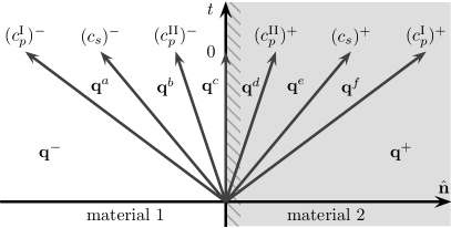
Figure 1: Schematic showing characteristic wave speeds at a poroelastic interface between two states $\mathbf{q}^{-}$ and $\mathbf{q}^{+}$. $\mathbf{q}^{a}$– $\mathbf{q}^{f}$ denote the intermediate states.

Thus:

$$\mathbf{q}^{-}-\mathbf{q}^{a} =\beta_{1}\mathbf{r}_{1}^{-}$$ (45)

$$\mathbf{q}^{a}-\mathbf{q}^{b} =\beta_{2}\mathbf{r}_{2}^{-}+\beta_{3}\mathbf{r}_{3}^{-}$$ (46)

$$\mathbf{q}^{b}-\mathbf{q}^{c} =\beta_{4}\mathbf{r}_{4}^{-}$$ (47)

$$\mathbf{q}^{d}-\mathbf{q}^{e} =\beta_{10}\mathbf{r}_{10}^{+}$$ (48)

$$\mathbf{q}^{e}-\mathbf{q}^{f} =\beta_{11}\mathbf{r}_{11}^{+}+\beta_{12}\mathbf{r}_{12}^{+}$$ (49)

$$\mathbf{q}^{f}-\mathbf{q}^{-} =\beta_{13}\mathbf{r}_{13}^{+}$$ (50)

where $\mathbf{r}_{j}^{\pm}$ is an eigenvector corresponding to wave speed $c_{j}^{\pm}$ and hence

$$\mathbf{q}^{-}-\mathbf{q}^{c} =\beta_{1}\mathbf{r}_{1}^{-}+\beta_{2}\mathbf{r}_{2}^{-}+\beta_{3}\mathbf{r}_{3}^{-}+\beta_{4}\mathbf{r}_{4}^{+}$$ (51)

$$\mathbf{q}^{d}-\mathbf{q}^{+} =\beta_{10}\mathbf{r}_{10}^{+}+\beta_{11}\mathbf{r}_{11}^{+}+\beta_{12}\mathbf{r}_{12}^{+}+\beta_{13}\mathbf{r}_{13}^{+}$$ (52)

Note that $\mathbf{r}_{4},\ldots,\mathbf{r}_{9}$ correspond to wavespeed zero and are not referenced in the following derivations.

We now make use of the orthogonality of the P-wave and the S-wave eigenvectors to uncouple the system (51) and (52). Recall that the eigenvectors $\mathbf{r}_{1}^{-},\mathbf{r}_{13}^{+}$ correspond to fast P-waves, $\mathbf{r}_{4}^{-},\mathbf{r}_{10}^{+}$ to slow P-waves, and $\mathbf{r}_{2}^{-},\mathbf{r}_{3}^{+}$, $\mathbf{r}_{11}^{+}$, $\mathbf{r}_{12}^{+}$ to S-waves. First we deal with the P-wave coefficients $\beta_{1},\beta_{3},\beta_{10},\beta_{13}$.

From the interface condition (41) we have

$$\Pi^{-}\mathbf{q}^{c}=\Pi^{+}\mathbf{q}^{d}$$

and so

$$L^{-1}\Pi^{-}\mathbf{q}^{c}=L^{-1}\Pi^{+}\mathbf{q}^{d}.$$

Using the first equality in (37) this gives

$$A^{-}(L^{-1}\mathbf{q}^{c})=A^{+}(L^{-1}\mathbf{q}^{d}),$$

that is

$$A^{-}(\mathbf{q}^{c})^{\prime}=A^{+}(\mathbf{q}^{d})^{\prime}.$$ (53)

Recalling that

$${\bf T}^{\pm}=2\mu_{\mathrm{fr}}^{\pm}{\bf E}+\lambda^{\pm}\operatorname{trace}({\bf E}){\bf I}-\alpha^{\pm}M^{\pm}\zeta{\bf I}$$

where $\displaystyle{\lambda^{\pm}=\kappa_{\mathrm{fr}}^{\pm}+\alpha^{2\pm}M^{\pm}-\frac{2}{3}\mu_{\mathrm{fr}}^{\pm}}$ and the $\pm$ indicates whether $\mathbf{T}$ is evaluated on the interior or exterior of the interface, it follows that

$$\hat{\mathbf{n}}^{\mathsf{T}}\mathbf{T}^{\pm}\hat{\mathbf{n}} =2\mu_{\mathrm{fr}}^{\pm}\hat{\mathbf{n}}^{\mathsf{T}}\mathbf{E}^{\pm}\hat{\mathbf{n}}+\lambda^{\pm}\operatorname{trace}(\mathbf{E}^{\pm})\hat{\mathbf{n}}^{\mathsf{T}}\mathbf{I}\hat{\mathbf{n}}-\alpha^{\pm}M^{\pm}\zeta^{\pm}\hat{\mathbf{n}}^{\mathsf{T}}\mathbf{I}\hat{\mathbf{n}}$$

$$=2\mu_{\mathrm{fr}}^{\pm}\hat{\mathbf{n}}^{\mathsf{T}}\mathbf{E}^{\pm}\hat{\mathbf{n}}+\lambda^{\pm}\operatorname{trace}(\mathbf{E}^{\pm})-\alpha^{\pm}M^{\pm}\zeta^{\pm}$$

$$=2\mu_{\mathrm{fr}}^{\pm}\hat{\mathbf{n}}^{\mathsf{T}}\mathbf{E}^{\pm}\hat{\mathbf{n}}+\lambda^{\pm}(\hat{\mathbf{n}}^{\mathsf{T}}\mathbf{E}^{\pm}\hat{\mathbf{n}}+\hat{\mathbf{s}}^{\mathsf{T}}\mathbf{E}^{\pm}\hat{\mathbf{s}}+\hat{\mathbf{t}}^{\mathsf{T}}\mathbf{E}^{\pm}\hat{\mathbf{t}})-\alpha^{\pm}M^{\pm}\zeta^{\pm}$$ (54)

since the trace is invariant under orthogonal transformations. We also have

$$\hat{\mathbf{s}}^{\mathsf{T}}\mathbf{T}^{\pm}\hat{\mathbf{n}}=2\mu_{\mathrm{fr}}\hat{\mathbf{s}}^{\mathsf{T}}\mathbf{E}^{\pm}\hat{\mathbf{n}},\quad\hat{\mathbf{t}}^{\mathsf{T}}\mathbf{T}^{\pm}\hat{\mathbf{s}}=2\mu_{\mathrm{fr}}\hat{\mathbf{t}}^{\mathsf{T}}\mathbf{E}^{\pm}\hat{\mathbf{s}},\quad\hat{\mathbf{t}}^{\mathsf{T}}\mathbf{T}^{\pm}\hat{\mathbf{n}}=2\mu_{\mathrm{fr}}\hat{\mathbf{t}}^{\mathsf{T}}\mathbf{E}^{\pm}\hat{\mathbf{n}}.$$ (55)

We obtain similarly for

$$\mathbf{T}_{\rm f}^{\pm}=M^{\pm}(\alpha^{\pm}\operatorname{trace}({\bf E}^{\pm})-\zeta^{\pm}){\bf I}$$

the following identity:

$$\hat{\mathbf{n}}^{\mathsf{T}}\mathbf{T}_{\rm f}^{\pm}\hat{\mathbf{n}} =M^{\pm}\alpha^{\pm}\operatorname{trace}(\mathbf{E}^{\pm})-M^{\pm}\zeta^{\pm}$$

$$=M^{\pm}\alpha^{\pm}(\hat{\mathbf{n}}^{\mathsf{T}}\mathbf{E}^{\pm}\hat{\mathbf{n}}+\hat{\mathbf{s}}^{\mathsf{T}}\mathbf{E}^{\pm}\hat{\mathbf{s}}+\hat{\mathbf{t}}^{\mathsf{T}}\mathbf{E}^{\pm}\hat{\mathbf{t}})-M^{\pm}\zeta^{\pm}.$$ (56)

Also

$$\hat{\mathbf{s}}^{\mathsf{T}}\mathbf{T}^{\pm}_{\rm f}\hat{\mathbf{n}}=\hat{\mathbf{t}}^{\mathsf{T}}\mathbf{T}^{\pm}_{\rm f}\hat{\mathbf{s}}=\hat{\mathbf{t}}^{\mathsf{T}}\mathbf{T}^{\pm}_{\rm f}\hat{\mathbf{n}}=0.$$ (57)

From (53) we obtain the following flux continuity relations

$$\hat{\mathbf{n}}\cdot\mathbf{v}_{\rm s}^{c} =\hat{\mathbf{n}}\cdot\mathbf{v}_{\rm s}^{d}$$ (58)

$$\hat{\mathbf{s}}\cdot\mathbf{v}_{\rm s}^{c} =\hat{\mathbf{s}}\cdot\mathbf{v}_{\rm s}^{d}$$ (59)

$$\hat{\mathbf{t}}\cdot\mathbf{v}_{\rm s}^{c} =\hat{\mathbf{t}}\cdot\mathbf{v}_{\rm s}^{d}$$ (60)

$$\hat{\mathbf{n}}\cdot\mathbf{v}_{\rm f}^{c} =\hat{\mathbf{n}}\cdot\mathbf{v}_{\rm f}^{d}$$ (61)

$$\hat{\mathbf{n}}^{\mathsf{T}}\mathbf{T}^{c}\hat{\mathbf{n}} =\hat{\mathbf{n}}^{\mathsf{T}}\mathbf{T}^{d}\hat{\mathbf{n}}$$ (62)

$$\hat{\mathbf{s}}^{\mathsf{T}}\mathbf{T}^{c}\hat{\mathbf{n}} =\hat{\mathbf{s}}^{\mathsf{T}}\mathbf{T}^{d}\hat{\mathbf{n}}$$ (63)

$$\hat{\mathbf{t}}^{\mathsf{T}}\mathbf{T}^{c}\hat{\mathbf{n}} =\hat{\mathbf{t}}^{\mathsf{T}}\mathbf{T}^{d}\hat{\mathbf{n}}$$ (64)

$$\hat{\mathbf{n}}^{\mathsf{T}}\mathbf{T}_{\rm f}^{c}\hat{\mathbf{n}} =\hat{\mathbf{n}}^{\mathsf{T}}\mathbf{T}_{\rm f}^{d}\hat{\mathbf{n}}$$ (65)

where we have used (54), (55) and (56).

We now proceed with the evaluation of the $\beta$ terms. From (51) we have

$$L^{-1}\mathbf{q}^{-}-L^{-1}\mathbf{q}^{c}=\beta_{1}(\mathbf{r}_{1}^{\prime})^{-}+\beta_{2}(\mathbf{r}_{2}^{\prime})^{-}+\beta_{3}(\mathbf{r}_{3}^{\prime})^{-}+\beta_{4}(\mathbf{r}_{4}^{\prime})^{-}$$

where the $(\mathbf{r}_{j}^{\prime})^{-}$ are the $j$’th columns of the eigenvector matrix $R$ given by equation (34) evaluated in the interior of an element. Unwrapping, and using (36), we obtain the relationships

$$\hat{\mathbf{n}}^{\mathsf{T}}\mathbf{E}^{-}\hat{\mathbf{n}}-\hat{\mathbf{n}}^{\mathsf{T}}\mathbf{E}^{c}\hat{\mathbf{n}} =\beta_{1}+\beta_{4}$$ (66)

$$\hat{\mathbf{s}}^{\mathsf{T}}\mathbf{E}^{-}\hat{\mathbf{s}} =\hat{\mathbf{s}}^{\mathsf{T}}\mathbf{E}^{c}\hat{\mathbf{s}}$$ (67)

$$\hat{\mathbf{t}}^{\mathsf{T}}\mathbf{E}^{-}\hat{\mathbf{t}} =\hat{\mathbf{t}}^{\mathsf{T}}\mathbf{E}^{c}\hat{\mathbf{t}}$$ (68)

$$\hat{\mathbf{s}}^{\mathsf{T}}\mathbf{E}^{-}\hat{\mathbf{n}}-\hat{\mathbf{s}}^{\mathsf{T}}\mathbf{E}^{c}\hat{\mathbf{n}} =\beta_{2}/2$$ (69)

$$\hat{\mathbf{t}}^{\mathsf{T}}\mathbf{E}^{-}\hat{\mathbf{s}} =\hat{\mathbf{t}}^{\mathsf{T}}\mathbf{E}^{c}\hat{\mathbf{s}}$$ (70)

$$\hat{\mathbf{t}}^{\mathsf{T}}\mathbf{E}^{-}\hat{\mathbf{n}}-\hat{\mathbf{t}}^{\mathsf{T}}\mathbf{E}^{c}\hat{\mathbf{n}} =\beta_{3}/2$$ (71)

$$\zeta^{-}-\zeta^{c} =-\gamma_{1}^{-}\beta_{1}-\gamma_{2}^{-}\beta_{4}$$ (72)

$$\hat{\mathbf{n}}\cdot\mathbf{v}_{\rm s}^{-}-\hat{\mathbf{n}}\cdot\mathbf{v}_{\rm s}^{c} =(c_{p}^{\mathrm{I}})^{-}\beta_{1}+(c_{p}^{\mathrm{II}})^{-}\beta_{4}$$ (73)

$$\hat{\mathbf{s}}\cdot\mathbf{v}_{\rm s}^{-}-\hat{\mathbf{s}}\cdot\mathbf{v}_{\rm s}^{c} =(c_{s})^{-}\beta_{2}$$ (74)

$$\hat{\mathbf{t}}\cdot\mathbf{v}_{\rm s}^{-}-\hat{\mathbf{t}}\cdot\mathbf{v}_{\rm s}^{c} =(c_{s})^{-}\beta_{3}$$ (75)

$$\hat{\mathbf{n}}\cdot\mathbf{v}_{\rm f}^{-}-\hat{\mathbf{n}}\cdot\mathbf{v}_{\rm f}^{c} =(\gamma_{1}c_{p}^{\mathrm{I}})^{-}\beta_{1}+(\gamma_{2}c_{p}^{\mathrm{II}})^{-}\beta_{4}$$ (76)

$$\hat{\mathbf{s}}\cdot\mathbf{v}_{\rm f}^{-}-\hat{\mathbf{s}}\cdot\mathbf{v}_{\rm f}^{c} =-(c_{s}\rho_{\mathrm{f}}/m)^{-}\beta_{2}$$ (77)

$$\hat{\mathbf{t}}\cdot\mathbf{v}_{\rm f}^{-}-\hat{\mathbf{t}}\cdot\mathbf{v}_{\rm f}^{c} =-(c_{s}\rho_{\mathrm{f}}/m)^{-}\beta_{3}$$ (78)

We derive similar relations on the right-hand side. From (52) we have

$$L^{-1}\mathbf{q}^{d}-L^{-1}\mathbf{q}^{+}=\beta_{10}(\mathbf{r}_{10}^{\prime})^{+}+\beta_{11}(\mathbf{r}_{11}^{\prime})^{+}+\beta_{12}(\mathbf{r}_{12}^{\prime})^{+}+\beta_{13}(\mathbf{r}_{13}^{\prime})^{+}$$

Thus:

$$\hat{\mathbf{n}}^{\mathsf{T}}\mathbf{E}^{d}\hat{\mathbf{n}}-\hat{\mathbf{n}}^{\mathsf{T}}\mathbf{E}^{+}\hat{\mathbf{n}} =\beta_{5}+\beta_{8}$$ (79)

$$\hat{\mathbf{s}}^{\mathsf{T}}\mathbf{E}^{d}\hat{\mathbf{s}} =\hat{\mathbf{s}}^{\mathsf{T}}\mathbf{E}^{+}\hat{\mathbf{s}}$$ (80)

$$\hat{\mathbf{t}}^{\mathsf{T}}\mathbf{E}^{d}\hat{\mathbf{t}} =\hat{\mathbf{t}}^{\mathsf{T}}\mathbf{E}^{+}\hat{\mathbf{t}}$$ (81)

$$\hat{\mathbf{s}}^{\mathsf{T}}\mathbf{E}^{d}\hat{\mathbf{n}}-\hat{\mathbf{s}}^{\mathsf{T}}\mathbf{E}^{+}\hat{\mathbf{n}} =\beta_{12}/2$$ (82)

$$\hat{\mathbf{t}}^{\mathsf{T}}\mathbf{E}^{d}\hat{\mathbf{s}} =\hat{\mathbf{t}}^{\mathsf{T}}\mathbf{E}^{+}\hat{\mathbf{s}}$$ (83)

$$\hat{\mathbf{t}}^{\mathsf{T}}\mathbf{E}^{d}\hat{\mathbf{n}}-\hat{\mathbf{t}}^{\mathsf{T}}\mathbf{E}^{+}\hat{\mathbf{n}} =\beta_{11}/2$$ (84)

$$\zeta^{d}-\zeta^{+} =-\gamma_{2}^{+}\beta_{10}-\gamma_{1}^{+}\beta_{13}$$ (85)

$$\hat{\mathbf{n}}\cdot\mathbf{v}_{\rm s}^{d}-\hat{\mathbf{n}}\cdot\mathbf{v}_{\rm s}^{+} =-(c_{p}^{\mathrm{II}})^{+}\beta_{10}-(c_{p}^{\mathrm{I}})^{+}\beta_{13}$$ (86)

$$\hat{\mathbf{s}}\cdot\mathbf{v}_{\rm s}^{d}-\hat{\mathbf{s}}\cdot\mathbf{v}_{\rm s}^{+} =-c_{s}^{+}\beta_{12}$$ (87)

$$\hat{\mathbf{t}}\cdot\mathbf{v}_{\rm s}^{d}-\hat{\mathbf{t}}\cdot\mathbf{v}_{\rm s}^{+} =-c_{s}^{+}\beta_{11}$$ (88)

$$\hat{\mathbf{n}}\cdot\mathbf{v}_{\rm f}^{d}-\hat{\mathbf{n}}\cdot\mathbf{v}_{\rm f}^{+} =-(\gamma_{2}c_{p}^{\mathrm{II}})^{+}\beta_{10}-(\gamma_{1}c_{p}^{\mathrm{I}})^{+}\beta_{13}$$ (89)

$$\hat{\mathbf{s}}\cdot\mathbf{v}_{\rm f}^{d}-\hat{\mathbf{s}}\cdot\mathbf{v}_{\rm f}^{+} =(c_{s}\rho_{\mathrm{f}}/m)^{+}\beta_{12}$$ (90)

$$\hat{\mathbf{t}}\cdot\mathbf{v}_{\rm f}^{d}-\hat{\mathbf{t}}\cdot\mathbf{v}_{\rm f}^{+} =(c_{s}\rho_{\mathrm{f}}/m)^{+}\beta_{11}.$$ (91)

Using the continuity condition (58), (73) and (86) we obtain

$$(c_{p}^{\mathrm{I}})^{-}\beta_{1}+(c_{p}^{\mathrm{II}})^{-}\beta_{4}-(c_{p}^{\mathrm{II}})^{+}\beta_{10}-(c_{p}^{\mathrm{I}})^{+}\beta_{13}=\hat{\mathbf{n}}\cdot(\mathbf{v}_{\rm s}^{-}-\mathbf{v}_{\rm s}^{+}).$$ (92)

Next from (61), (76) and (89) we obtain

$$(\gamma_{1}c_{p}^{\mathrm{I}})^{-}\beta_{1}+(\gamma_{2}c_{p}^{\mathrm{II}})^{-}\beta_{4}-(\gamma_{2}c_{p}^{\mathrm{II}})^{+}\beta_{10}-(\gamma_{1}c_{p}^{\mathrm{I}})^{+}\beta_{13}=\hat{\mathbf{n}}\cdot(\mathbf{v}_{\rm f}^{-}-\mathbf{v}_{\rm f}^{+}).$$ (93)

Using the continuity condition (62) and the identity (54) we obtain

$$2\mu_{\mathrm{fr}}^{-}\hat{\mathbf{n}}^{\mathsf{T}}\mathbf{E}^{c}\hat{\mathbf{n}}+\lambda^{-}(\hat{\mathbf{n}}^{\mathsf{T}}\mathbf{E}^{c}\hat{\mathbf{n}}+\hat{\mathbf{s}}^{\mathsf{T}}\mathbf{E}^{c}\hat{\mathbf{s}}+\hat{\mathbf{t}}^{\mathsf{T}}\mathbf{E}^{c}\hat{\mathbf{t}})-\alpha^{-}M^{-}\zeta^{c}=2\mu_{\mathrm{fr}}^{+}\hat{\mathbf{n}}^{\mathsf{T}}\mathbf{E}^{d}\hat{\mathbf{n}}+\lambda^{+}(\hat{\mathbf{n}}^{\mathsf{T}}\mathbf{E}^{d}\hat{\mathbf{n}}+\hat{\mathbf{s}}^{\mathsf{T}}\mathbf{E}^{d}\hat{\mathbf{s}}+\hat{\mathbf{t}}^{\mathsf{T}}\mathbf{E}^{c}\hat{\mathbf{t}})-\alpha^{+}M^{+}\zeta^{d}$$ (94)

We now substitute for $\mathbf{E}^{c}$ and $\mathbf{E}^{d}$ using (66), (67), (72), (79), (80) and (85)

$$(2\mu_{\mathrm{fr}}^{-}+\lambda^{-}+\alpha^{-}M^{-}\gamma_{1}^{-})\beta_{1}+(2\mu_{\mathrm{fr}}^{-}+\lambda^{-}+\alpha^{-}M^{-}\gamma_{2}^{-})\beta_{4}+(2\mu_{\mathrm{fr}}^{+}+\lambda^{+}+\alpha^{+}M^{+}\gamma_{2}^{+})\beta_{10}\\ +(2\mu_{\mathrm{fr}}^{+}+\lambda^{+}+\alpha^{+}M^{+}\gamma_{1}^{+})\beta_{13}=\hat{\mathbf{n}}^{\mathsf{T}}(\mathbf{T}^{-}-\mathbf{T}^{+})\hat{\mathbf{n}}.$$ (95)

Finally using the continuity condition (65) and the identity (56) we obtain

$$M^{-}\alpha^{-}(\hat{\mathbf{n}}^{\mathsf{T}}\mathbf{E}^{c}\hat{\mathbf{n}}+\hat{\mathbf{s}}^{\mathsf{T}}\mathbf{E}^{c}\hat{\mathbf{s}})-M^{-}\zeta^{c}=M^{+}\alpha^{+}(\hat{\mathbf{n}}^{\mathsf{T}}\mathbf{E}^{d}\hat{\mathbf{n}}+\hat{\mathbf{s}}^{\mathsf{T}}\mathbf{E}^{d}\hat{\mathbf{s}})-M^{+}\zeta^{d}.$$

Substituting again for $\mathbf{E}^{c}$ and $\mathbf{E}^{d}$ gives

$$M^{-}(\alpha^{-}+\gamma_{1}^{-})\beta_{1}+M^{-}(\alpha^{-}+\gamma_{2}^{-})\beta_{4}+M^{+}(\alpha^{+}+\gamma_{2}^{+})\beta_{10}+M^{+}(\alpha^{+}+\gamma_{1}^{+})\beta_{13}=\hat{\mathbf{n}}^{\mathsf{T}}(\mathbf{T}_{\rm f}^{-}-\mathbf{T}_{\rm f}^{+})\hat{\mathbf{n}}.$$ (96)

There is no straightforward solution to the system (92)–(96). Inverting the coefficient matrix

$$\begin{pmatrix}2\mu_{\mathrm{fr}}^{-}+\lambda^{-}+\alpha^{-}M^{-}\gamma_{1}^{-}&2\mu_{\mathrm{fr}}^{-}+\lambda^{-}+\alpha^{-}M^{-}\gamma_{2}^{-}&2\mu_{\mathrm{fr}}^{+}+\lambda^{+}+\alpha^{+}M^{+}\gamma_{2}^{+}&2\mu_{\mathrm{fr}}^{+}+\lambda^{+}+\alpha^{+}M^{+}\gamma_{1}^{+}\\ M^{-}(\alpha^{-}+\gamma_{1}^{-})&M^{-}(\alpha^{-}+\gamma_{2}^{-})&M^{+}(\alpha^{+}+\gamma_{2}^{+})&M^{+}(\alpha^{+}+\gamma_{1}^{+})\\ (c_{p}^{\mathrm{I}})^{-}&(c_{p}^{\mathrm{II}})^{-}&-(c_{p}^{\mathrm{II}})^{+}&-(c_{p}^{\mathrm{I}})^{+}\\ (\gamma_{1}c_{p}^{\mathrm{I}})^{-}&(\gamma_{2}c_{p}^{\mathrm{II}})^{-}&-(\gamma_{2}c_{p}^{\mathrm{II}})^{+}&-(\gamma_{1}c_{p}^{\mathrm{I}})^{+}\end{pmatrix}$$

we obtain the following expressions:

$$\beta_{1} =d_{11}\hat{\mathbf{n}}^{\mathsf{T}}(\mathbf{T}^{-}-\mathbf{T}^{+})\hat{\mathbf{n}}+d_{12}\hat{\mathbf{n}}^{\mathsf{T}}(\mathbf{T}_{\rm f}^{-}-\mathbf{T}_{\rm f}^{+})\hat{\mathbf{n}}+d_{13}\hat{\mathbf{n}}\cdot(\mathbf{v}_{\rm s}^{-}-\mathbf{v}_{\rm s}^{+})+d_{14}\hat{\mathbf{n}}\cdot(\mathbf{v}_{\rm f}^{-}-\mathbf{v}_{\rm f}^{+})$$ (97)

$$\beta_{4} =d_{21}\hat{\mathbf{n}}^{\mathsf{T}}(\mathbf{T}^{-}-\mathbf{T}^{+})\hat{\mathbf{n}}+d_{22}\hat{\mathbf{n}}^{\mathsf{T}}(\mathbf{T}_{\rm f}^{-}-\mathbf{T}_{\rm f}^{+})\hat{\mathbf{n}}+d_{23}\hat{\mathbf{n}}\cdot(\mathbf{v}_{\rm s}^{-}-\mathbf{v}_{\rm s}^{+})+d_{24}\hat{\mathbf{n}}\cdot(\mathbf{v}_{\rm f}^{-}-\mathbf{v}_{\rm f}^{+})$$ (98)

$$\beta_{5} =d_{31}\hat{\mathbf{n}}^{\mathsf{T}}(\mathbf{T}^{-}-\mathbf{T}^{+})\hat{\mathbf{n}}+d_{32}\hat{\mathbf{n}}^{\mathsf{T}}(\mathbf{T}_{\rm f}^{-}-\mathbf{T}_{\rm f}^{+})\hat{\mathbf{n}}+d_{33}\hat{\mathbf{n}}\cdot(\mathbf{v}_{\rm s}^{-}-\mathbf{v}_{\rm s}^{+})+d_{34}\hat{\mathbf{n}}\cdot(\mathbf{v}_{\rm f}^{-}-\mathbf{v}_{\rm f}^{+})$$ (99)

$$\beta_{8} =d_{41}\hat{\mathbf{n}}^{\mathsf{T}}(\mathbf{T}^{-}-\mathbf{T}^{+})\hat{\mathbf{n}}+d_{42}\hat{\mathbf{n}}^{\mathsf{T}}(\mathbf{T}_{\rm f}^{-}-\mathbf{T}_{\rm f}^{+})\hat{\mathbf{n}}+d_{43}\hat{\mathbf{n}}\cdot(\mathbf{v}_{\rm s}^{-}-\mathbf{v}_{\rm s}^{+})+d_{44}\hat{\mathbf{n}}\cdot(\mathbf{v}_{\rm f}^{-}-\mathbf{v}_{\rm f}^{+})$$ (100)

Here the $d_{ij}$ are the entries of the inverse of the coefficient matrix above.

Now we deal with the shear waves. Using the continuity condition (63) with the identity (55)

$$2\mu_{\mathrm{fr}}^{-}\hat{\mathbf{s}}^{\mathsf{T}}\mathbf{E}^{c}\hat{\mathbf{n}}=2\mu_{\mathrm{fr}}^{+}\hat{\mathbf{s}}^{\mathsf{T}}\mathbf{E}^{d}\hat{\mathbf{n}}.$$ (101)

Substituting for $\mathbf{E}^{c}$ and $\mathbf{E}^{d}$ using (69) and (82)

$$(\mu_{\mathrm{fr}})^{-}\beta_{2}+(\mu_{\mathrm{fr}})^{+}\beta_{12}=\hat{\mathbf{s}}^{\mathsf{T}}(\mathbf{T}^{-}-\mathbf{T}^{+})\hat{\mathbf{n}}.$$ (102)

Finally using (59), (74) and (87) gives

$$(c_{s})^{-}\beta_{2}-(c_{s})^{+}\beta_{12}=\hat{\mathbf{s}}\cdot(\mathbf{v}_{\rm s}^{-}-\mathbf{v}_{\rm s}^{+}).$$ (103)

Therefore,

$$\beta_{2} =\frac{(c_{s})^{+}\hat{\mathbf{s}}^{\mathsf{T}}(\mathbf{T}^{-}-\mathbf{T}^{+})\hat{\mathbf{n}}+\mu_{\mathrm{fr}}^{+}\hat{\mathbf{s}}\cdot(\mathbf{v}_{\rm s}^{-}-\mathbf{v}_{\rm s}^{+})}{(c_{s})^{+}(\mu_{\mathrm{fr}})^{-}+(c_{s})^{-}(\mu_{\mathrm{fr}})^{+}}$$ (104)

$$\beta_{12} =\frac{(c_{s})^{-}\hat{\mathbf{s}}^{\mathsf{T}}(\mathbf{T}^{-}-\mathbf{T}^{+})\hat{\mathbf{n}}-\mu_{\mathrm{fr}}^{-}\hat{\mathbf{s}}\cdot(\mathbf{v}_{\rm s}^{-}-\mathbf{v}_{\rm s}^{+})}{(c_{s})^{+}(\mu_{\mathrm{fr}})^{-}+(c_{s})^{-}(\mu_{\mathrm{fr}})^{+}}.$$ (105)

In a similar manner using the continuity relationships (63) we obtain

$$\beta_{3} =\frac{(c_{s})^{+}\hat{\mathbf{t}}^{\mathsf{T}}(\mathbf{T}^{-}-\mathbf{T}^{+})\hat{\mathbf{n}}+\mu_{\mathrm{fr}}^{+}\hat{\mathbf{t}}\cdot(\mathbf{v}_{\rm s}^{-}-\mathbf{v}_{\rm s}^{+})}{(c_{s})^{+}(\mu_{\mathrm{fr}})^{-}+(c_{s})^{-}(\mu_{\mathrm{fr}})^{+}}$$ (106)

$$\beta_{11} =\frac{(c_{s})^{-}\hat{\mathbf{t}}^{\mathsf{T}}(\mathbf{T}^{-}-\mathbf{T}^{+})\hat{\mathbf{n}}-\mu_{\mathrm{fr}}^{-}\hat{\mathbf{t}}\cdot(\mathbf{v}_{\rm s}^{-}-\mathbf{v}_{\rm s}^{+})}{(c_{s})^{+}(\mu_{\mathrm{fr}})^{-}+(c_{s})^{-}(\mu_{\mathrm{fr}})^{+}}.$$ (107)

3.5 Upwind numerical flux

We define an upwind numerical flux $(\Pi\mathbf{q})^{*}$ along $\hat{\mathbf{n}}$ by

$$(\Pi\mathbf{q})^{*}=\Pi^{-}\mathbf{q}^{-}+Q^{-}(\beta_{1}(c_{p}^{\mathrm{I}})^{-}\mathbf{r}_{1}^{-}+\beta_{2}(c_{s})^{-}\mathbf{r}_{2}^{-}+\beta_{3}(c_{s})^{-}\mathbf{r}_{3}^{-}+\beta_{4}(c_{p}^{\mathrm{II}})^{-}\mathbf{r}_{4}^{-}).$$ (108)

We now compute the $\beta_{i}\mathbf{r}_{i}$ terms. First, noting that $\mathbf{r}_{i}=L\mathbf{r}_{i}^{\prime}$, a simple computation gives

$$\mathbf{r}_{1}^{-}=\begin{pmatrix}\overline{\hat{\mathbf{n}}\otimes\hat{\mathbf{n}}}\\ -\gamma_{1}^{-}\\ (c_{p}^{\mathrm{I}})^{-}\hat{\mathbf{n}}\\ \gamma_{1}^{-}(c_{p}^{\mathrm{I}})^{-}\hat{\mathbf{n}}\end{pmatrix},\quad\mathbf{r}_{2}^{-}=\begin{pmatrix}\overline{\hat{\mathbf{n}}\otimes\hat{\mathbf{s}}}\\ 0\\ (c_{s})^{-}\hat{\mathbf{s}}\\ -\frac{(c_{s})^{-}\rho_{\mathrm{f}}^{-}}{m^{-}}\hat{\mathbf{s}}\end{pmatrix},\quad\mathbf{r}_{3}^{-}=\begin{pmatrix}\overline{\hat{\mathbf{n}}\otimes\hat{\mathbf{t}}}\\ 0\\ (c_{s})^{-}\hat{\mathbf{t}}\\ -\frac{(c_{s})^{-}\rho_{\mathrm{f}}^{-}}{m^{-}}\hat{\mathbf{t}}\end{pmatrix},\quad\mathbf{r}_{4}^{-}=\begin{pmatrix}\overline{\hat{\mathbf{n}}\otimes\hat{\mathbf{n}}}\\ -\gamma_{2}^{-}\\ (c_{p}^{\mathrm{II}})^{-}\hat{\mathbf{n}}\\ \gamma_{2}^{-}(c_{p}^{\mathrm{II}})^{-}\hat{\mathbf{n}}\end{pmatrix},$$

where $\overline{\hat{\mathbf{n}}\otimes\hat{\mathbf{n}}}=(n_{1}^{2},n_{2}^{2},n_{3}^{2},n_{1}n_{2},n_{2}n_{3},n_{1}n_{3})^{\mathsf{T}}$ is a flattened representation of the tensor $\hat{\mathbf{n}}\otimes\hat{\mathbf{n}}$, etc.

In what follows, we make multiple use of the vector/tensor identities

$$(\hat{\mathbf{s}}\cdot\mathbf{a})\hat{\mathbf{s}}+(\hat{\mathbf{t}}\cdot\mathbf{a})\hat{\mathbf{t}} =-\hat{\mathbf{n}}\times(\hat{\mathbf{n}}\times\mathbf{a})$$ (109)

$$(\hat{\mathbf{s}}\cdot\mathbf{a})\operatorname{sym}(\hat{\mathbf{s}}\otimes\hat{\mathbf{n}})+(\hat{\mathbf{t}}\cdot\mathbf{a})\operatorname{sym}(\hat{\mathbf{t}}\otimes\hat{\mathbf{n}}) =-\operatorname{sym}(\hat{\mathbf{n}}\otimes(\hat{\mathbf{n}}\times(\hat{\mathbf{n}}\times\mathbf{a})))$$ (110)

We define

$$[\![\mathbf{T}]\!] =\mathbf{T}^{-}\hat{\mathbf{n}}^{-}+\mathbf{T}^{+}\hat{\mathbf{n}}^{+}$$

$$[\![\mathbf{T}_{\rm f}]\!] =\mathbf{T}_{\rm f}^{-}\hat{\mathbf{n}}^{-}+\mathbf{T}_{\rm f}^{+}\hat{\mathbf{n}}^{+}$$

$$[\![\mathbf{v}]\!] =\hat{\mathbf{n}}^{-}{}^{\mathsf{T}}\mathbf{v}^{-}+\hat{\mathbf{n}}^{+}{}^{\mathsf{T}}\mathbf{v}^{+}$$

$$[\mathbf{v}] =\mathbf{v}^{-}-\mathbf{v}^{+}$$

For the fast P-wave term we have

$$\beta_{1}(c_{p}^{\mathrm{I}})^{-}\mathbf{r}_{1}^{-}=(c_{p}^{\mathrm{I}})^{-}(d_{11}\hat{\mathbf{n}}^{\mathsf{T}}[\![\mathbf{T}]\!]+d_{12}\hat{\mathbf{n}}^{\mathsf{T}}[\![\mathbf{T}_{\rm f}]\!]+d_{13}[\![\mathbf{v}_{\rm s}]\!]+d_{14}[\![\mathbf{v}_{\rm f}]\!])\times\\ \begin{pmatrix}\overline{\hat{\mathbf{n}}\otimes\hat{\mathbf{n}}}\\ -\gamma_{1}^{-}\\ (c_{p}^{\mathrm{I}})^{-}\hat{\mathbf{n}}\\ \gamma_{1}^{-}(c_{p}^{\mathrm{I}})^{-}\hat{\mathbf{n}}\end{pmatrix},$$ (111)

For the S-wave term we have

$$\beta_{2}c_{s}^{-}\mathbf{r}_{2}^{-}+\beta_{3}c_{s}^{-}\mathbf{r}_{3}^{-}=\frac{-(c_{s})^{-}(c_{s})^{+}}{(c_{s})^{+}(\mu_{\mathrm{fr}})^{-}+(c_{s})^{-}(\mu_{\mathrm{fr}})^{+}}\begin{pmatrix}\overline{\operatorname{sym}(\hat{\mathbf{n}}\otimes(\hat{\mathbf{n}}\times(\hat{\mathbf{n}}\times[\![\mathbf{T}]\!])))}\\ 0\\ (c_{s})^{-}\hat{\mathbf{n}}\times(\hat{\mathbf{n}}\times[\![\mathbf{T}]\!])\\ \frac{-(c_{s})^{-}\rho_{f}^{-}}{m^{-}}\hat{\mathbf{n}}\times(\hat{\mathbf{n}}\times[\![\mathbf{T}]\!])\end{pmatrix}\\ -\frac{(c_{s})^{-}(\mu_{\mathrm{fr}})^{+}}{(c_{s})^{+}(\mu_{\mathrm{fr}})^{-}+(c_{s})^{-}(\mu_{\mathrm{fr}})^{+}}\begin{pmatrix}\overline{\operatorname{sym}(\hat{\mathbf{n}}\otimes(\hat{\mathbf{n}}\times(\hat{\mathbf{n}}\times[\![\mathbf{v}_{\rm s}]\!])))}\\ 0\\ (c_{s})^{-}\hat{\mathbf{n}}\times(\hat{\mathbf{n}}\times[\mathbf{v}_{\rm s}])\\ \frac{-(c_{s})^{-}\rho_{f}^{-}}{m^{-}}\hat{\mathbf{n}}\times(\hat{\mathbf{n}}\times[\mathbf{v}_{\rm s}])\end{pmatrix}$$ (112)

Finally for the slow P-wave we have

$$\beta_{3}(c_{p}^{\mathrm{II}})^{-}\mathbf{r}_{1}^{-}=(c_{p}^{\mathrm{II}})^{-}(d_{21}\hat{\mathbf{n}}^{\mathsf{T}}[\![\mathbf{T}]\!]+d_{22}\hat{\mathbf{n}}^{\mathsf{T}}[\![\mathbf{T}_{\rm f}]\!]+d_{23}[\![\mathbf{v}_{\rm s}]\!]+d_{24}[\![\mathbf{v}_{\rm f}]\!])\times\\ \begin{pmatrix}\overline{\hat{\mathbf{n}}\otimes\hat{\mathbf{n}}}\\ -\gamma_{2}^{-}\\ (c_{p}^{\mathrm{II}})^{-}\hat{\mathbf{n}}\\ \gamma_{2}^{-}(c_{p}^{\mathrm{II}})^{-}\hat{\mathbf{n}}\end{pmatrix}$$ (113)

4 Consideration of poro-viscoelasticity

4.1 Introduction

The low-frequency regime is straightforward and follows Biot’s 1956 paper [3]. Using the conventions of equations (1) and (2), the low-frequency dissipative regime is modelled by the term $\displaystyle{\frac{\eta}{k}\frac{\partial\mathbf{w}}{\partial t}}$. For the hyperbolic system (21) we simply add the source term (25). We note that in certain physical situations (when the permeability of the solid matrix is very small and the frequency content of the propagating wave very low) the second P-wave can be essentially static and highly diffusive (so has a characteristic timescale much smaller than the time step of the non-dissipative hyperbolic system), rendering the system stiff and requiring extremely small time steps in an explicit scheme to capture the dissipative effects. This is considered by Carcione and Quiroga-Goode in [8] who used an operator splitting approach to avoid this issue and treated the viscous dissipation term analytically. In a more recent paper Lemoine et al. [22] work in a finite volume setting and again implement an operator splitting on the dissipative part, while an IMEX scheme is implemented in [12]. Here we consider both operator-splitting and IMEX techniques; see Section 7 below.

4.2 High-frequency case

In the high-frequency case the term $\displaystyle{\frac{\eta}{k}\frac{\partial\mathbf{w}}{\partial t}}$ in equation (2) is replaced by a convolution $\displaystyle{b*\frac{\partial^{2}\mathbf{w}}{\partial t^{2}}}$ where $b(t)=\frac{\eta}{k}\Psi(t)H(t)$, $\Psi(t)$ is a relaxation function of the form

$$\Psi(t)=1+\sum_{l=1}^{L}\left(\frac{\tau_{\epsilon}^{l}}{\tau_{\sigma}^{l}}-1\right)e^{-t/\tau_{\sigma}^{l}}$$ (114)

with relaxation times $\tau_{\epsilon}$ and $\tau_{\sigma}$, and $H(t)$ is a Heaviside function. Thus the relaxation mechanism corresponds to a generalised Zener model; see [7]. In practice it is common to deal with a single Zener model, which is the case we deal with here. We have

$$b*\frac{\partial\mathbf{v}_{\rm f}}{\partial t} =\frac{\eta}{k}\int_{-\infty}^{t}\Psi(t-\tau)\frac{\partial\mathbf{v}_{\rm f}}{\partial\tau}d\tau$$ (115)

$$=\frac{\eta}{k}\int_{-\infty}^{t}\frac{\partial\mathbf{v}_{\rm f}}{\partial\tau}d\tau+\frac{\eta}{k}\sum_{l=1}^{L}\left(\frac{\tau_{\epsilon}^{l}}{\tau_{\sigma}^{l}}-1\right)\int_{-\infty}^{t}e^{-(t-\tau)/\tau_{\sigma}^{l}}\frac{\partial\mathbf{v}_{\rm f}}{\partial\tau}d\tau$$ (116)

$$=\frac{\eta}{k}\mathbf{v}_{\rm f}+\frac{\eta}{k}\sum_{l=1}^{L}\left(\frac{\tau_{\epsilon}^{l}}{\tau_{\sigma}^{l}}-1\right)\int_{-\infty}^{t}e^{-(t-\tau)/\tau_{\sigma}^{l}}\frac{\partial\mathbf{v}_{\rm f}}{\partial\tau}d\tau$$ (117)

Introducing memory variables

$$\mathbf{e}^{l}=\left(\frac{\tau_{\epsilon}^{l}}{\tau_{\sigma}^{l}}-1\right)\int_{-\infty}^{t}e^{-(t-\tau)/\tau_{\sigma}^{l}}\frac{\partial\mathbf{v}_{\rm f}}{\partial\tau}d\tau$$ (118)

we obtain $3L$ additional differential equations:

$$\frac{\partial\mathbf{e}^{l}}{\partial t} =\left(\frac{\tau_{\epsilon}^{l}}{\tau_{\sigma}^{l}}-1\right)\frac{\partial\mathbf{v}_{\rm f}}{\partial t}-\frac{\mathbf{e}^{l}}{\tau_{\sigma}^{l}}$$ (119)

and

$$b*\frac{\partial\mathbf{v}_{\rm f}}{\partial t}=\frac{\eta}{k}\mathbf{v}_{\rm f}+\frac{\eta}{k}\sum_{l=1}^{L}\mathbf{e}^{l}.$$ (120)

It is customary to express the relaxation times in terms of a quality factor $Q_{0}$ and a reference frequency $f_{0}$ as

$$\tau_{\epsilon} =(\sqrt{Q_{0}^{2}+1}+1)/(2\pi f_{0}Q_{0})$$ (121)

$$\tau_{\sigma} =(\sqrt{Q_{0}^{2}+1}-1)/(2\pi f_{0}Q_{0}).$$ (122)

For $L=1$ the variable $\mathbf{q}$ defined in (15) must now be augmented with three additional variables $e^{1}_{x},e^{1}_{y},e^{1}_{z}$:

$$\mathbf{q}=(\epsilon_{11},\epsilon_{22},\epsilon_{33},\epsilon_{12},\epsilon_{23},\epsilon_{13},\zeta,u_{\rm s},v_{\rm s},w_{\rm s},u_{\rm f},v_{\rm f},w_{\rm f},e^{1}_{x},e^{1}_{y},e^{1}_{z})^{\mathsf{T}}$$ (123)

and the various coefficient matrices inflated in an obvious manner.

As noted in [12] implementation of the high-frequency case needs to be carried out with some care. Solving the sixteen-variable system as an inflated hyperbolic system results in a memory variable that converges to zero very quickly. An accurate scheme is obtained by treating the memory equations (119) as an uncoupled system of ordinary differential equations and evaluating $\displaystyle{\frac{\partial\mathbf{v}_{\rm f}}{\partial t}}$ from its gradient and flux terms.

5 Elastic/poroelastic coupling

In many applications to geophysics, one is interested in coupling elastic and poroelastic wave propagation; see [19, 20, 21]. In this section we outline the DG discretisation for three-dimensional elastic waves for an isotropic medium, again for a velocity/strain formulation. This results for the elastic case were given in [29], and are simply summarised below for convenience and consistency with the conventions of this paper. We then derive numerical fluxes for the interface between elastic and poroelastic elements.

Expressed as a second-order system the elastic wave equation takes the form

$$\rho_{\mathrm{e}}\frac{\partial^{2}\mathbf{u}_{\rm e}}{\partial t^{2}}=\nabla\cdot\mathbf{S}$$ (124)

where $\rho_{\mathrm{e}}$ is density and $\mathbf{S}$ is a stress tensor. In the isotropic case we consider here $\mathbf{S}$ may be written in the usual form

$$\mathbf{S}=2\mu_{\mathrm{e}}{\bf E}+\lambda_{\mathrm{e}}\operatorname{trace}({\bf E}){\bf I}$$ (125)

where ${\bf E}$ is the solid strain tensor and $\mu_{\mathrm{e}}$ and $\lambda_{\mathrm{e}}$ are Lamé coefficients. Expressed as a first-order hyperbolic system with variable

$$\mathbf{q}_{e}=(\epsilon_{11},\epsilon_{22},\epsilon_{33},\epsilon_{12},\epsilon_{23},\epsilon_{13},u_{\rm e},v_{\rm e},w_{\rm e})^{\mathsf{T}}$$ (126)

where $\mathbf{v}_{\rm e}=(u_{\rm e},v_{\rm e},w_{\rm e})$ are the $x$, $y$ and $z$ components of the velocity $\displaystyle{\frac{\partial\mathbf{u}_{\rm e}}{\partial t}}$ gives

$$Q_{e}\frac{\partial\mathbf{q}}{\partial t}+\nabla\cdot\mathcal{F}_{e}=Q_{e}\frac{\partial\mathbf{q}}{\partial t}+\frac{\partial(A_{e}^{i}\mathbf{q})}{\partial x_{i}}=0$$ (127)

where

$$\mathcal{F}_{e}=[F_{1},F_{2},F_{3}]=[A_{e}^{1}\mathbf{q},A_{e}^{2}\mathbf{q},A_{e}^{3}\mathbf{q}],$$

and

$$Q_{e}=\left(\begin{array}[]{c|c}I&0\\ \hline\cr 0&Q_{e,2}\\ \end{array}\right)$$ (128)

(here $I$ is the $6\times 6$ identity matrix) and

$$Q_{e,2}=\begin{pmatrix}\rho_{\mathrm{e}}&0&0\\ 0&\rho_{\mathrm{e}}&0\\ 0&0&\rho_{\mathrm{e}}\end{pmatrix}.$$ (129)

As in equation (24) the off-diagonal blocks of the Jacobian matrices $A_{e}^{i}$, $i=1,2,3$ are given in Table 2.

Table 2: The off-diagonal blocks of the Jacobian matrices $A_{e}^{i}$.

$$A_{e,1}^{1} =-\begin{pmatrix}2\mu_{\mathrm{e}}+\lambda_{\mathrm{e}}&\lambda_{\mathrm{e}}&\lambda_{\mathrm{e}}&0&0&0\\ 0&0&0&2\mu_{\mathrm{e}}&0&0\\ 0&0&0&0&0&2\mu_{\mathrm{e}}\end{pmatrix}, A_{e,2}^{1}=-\begin{pmatrix}1&0&0\\ 0&0&0\\ 0&0&0\\ 0&1/2&0\\ 0&0&0\\ 0&0&1/2\\ \end{pmatrix}$$

$$A_{e,1}^{2} =-\begin{pmatrix}0&0&0&2\mu_{\mathrm{e}}&0&0\\ \lambda_{\mathrm{e}}&2\mu_{\mathrm{e}}+\lambda_{\mathrm{e}}&\lambda_{\mathrm{e}}&0&0&0\\ 0&0&0&0&2\mu_{\mathrm{e}}&0\\ \end{pmatrix} A_{e,2}^{2}=-\begin{pmatrix}0&0&0\\ 0&1&0\\ 0&0&0\\ 1/2&0&0\\ 0&0&1/2\\ 0&0&0\\ \end{pmatrix}$$

$$A_{e,1}^{3} =-\begin{pmatrix}0&0&0&0&0&2\mu_{\mathrm{e}}\\ 0&0&0&0&2\mu_{\mathrm{e}}&0\\ \lambda_{\mathrm{e}}&\lambda_{\mathrm{e}}&2\mu_{\mathrm{e}}+\lambda_{\mathrm{e}}&0&0&0\\ \end{pmatrix} A_{e,2}^{2}=-\begin{pmatrix}0&0&0\\ 0&0&0\\ 0&0&1\\ 0&0&0\\ 0&1/2&0\\ 1/2&0&0\\ \end{pmatrix}$$

We have the well-known expressions for elastic wave speeds

$$c_{p}=\pm\sqrt{\frac{\lambda_{\mathrm{e}}+2\mu_{\mathrm{e}}}{\rho_{\mathrm{e}}}}\quad\text{and}\quad c_{s}=\pm\sqrt{\frac{\mu_{\mathrm{e}}}{\rho_{\mathrm{e}}}}.$$ (130)

Solving the Riemann problem as before we obtain the following coefficients corresponding to the non-zero wave speeds

$$\beta_{1} =\frac{(c_{p})^{+}\hat{\mathbf{n}}^{\mathsf{T}}(\mathbf{S}^{-}-\mathbf{S}^{+})\hat{\mathbf{n}}+(\lambda_{\mathrm{e}}^{+}+2\mu_{\mathrm{e}}^{+})\hat{\mathbf{n}}\cdot(\mathbf{v}_{\rm e}^{-}-\mathbf{v}_{\rm e}^{+})}{(c_{p})^{+}(\lambda_{\mathrm{e}}^{-}+2\mu_{\mathrm{e}}^{-})+(c_{p})^{-}(\lambda_{\mathrm{e}}^{+}+2\mu_{\mathrm{e}}^{+})}$$ (131)

$$\beta_{2} =\frac{(c_{s})^{+}\hat{\mathbf{s}}^{\mathsf{T}}(\mathbf{S}^{-}-\mathbf{S}^{+})\hat{\mathbf{n}}+\mu_{\mathrm{e}}^{+}\hat{\mathbf{s}}\cdot(\mathbf{v}_{\rm e}^{-}-\mathbf{v}_{\rm e}^{+})}{(c_{s})^{+}(\mu_{\mathrm{e}})^{-}+(c_{s})^{-}(\mu_{\mathrm{e}})^{+}}$$ (132)

$$\beta_{3} =\frac{(c_{s})^{-}\hat{\mathbf{t}}^{\mathsf{T}}(\mathbf{S}^{-}-\mathbf{S}^{+})\hat{\mathbf{n}}+\mu_{\mathrm{e}}^{-}\hat{\mathbf{t}}\cdot(\mathbf{v}_{\rm e}^{-}-\mathbf{v}_{\rm e}^{+})}{(c_{s})^{+}(\mu_{\mathrm{e}})^{-}+(c_{s})^{-}(\mu_{\mathrm{e}})^{+}}$$ (133)

Defining an upwind numerical flux $(\Pi\mathbf{q})^{*}$ along $\hat{\mathbf{n}}$ by

$$(\Pi\mathbf{q})^{*}=\Pi^{-}\mathbf{q}^{-}+Q^{-}(\beta_{1}(c_{p})^{-}\mathbf{r}_{1}^{-}+\beta_{2}(c_{s})^{-}\mathbf{r}_{2}^{-}+\beta_{3}(c_{s})^{-}\mathbf{r}_{3}^{-})$$ (135)

where

$$\mathbf{r}_{1}^{-}=\begin{pmatrix}\overline{\hat{\mathbf{n}}\otimes\hat{\mathbf{n}}}\\ (c_{p})^{-}\hat{\mathbf{n}}\end{pmatrix},\quad\mathbf{r}_{2}^{-}=\begin{pmatrix}\overline{\hat{\mathbf{n}}\otimes\hat{\mathbf{s}}}\\ (c_{s})^{-}\hat{\mathbf{s}}\end{pmatrix},\quad\mathbf{r}_{3}^{-}=\begin{pmatrix}\overline{\hat{\mathbf{n}}\otimes\hat{\mathbf{t}}}\\ (c_{s})^{-}\hat{\mathbf{t}}\end{pmatrix},$$

where $\hat{\mathbf{n}}=(\hat{n}_{1},\hat{n}_{2},\hat{n}_{3})^{\mathsf{T}}$, $\hat{\mathbf{s}}=(\hat{s}_{1},\hat{s}_{2},\hat{s}_{3})^{\mathsf{T}}$ and $\hat{\mathbf{t}}=(\hat{t}_{1},\hat{t}_{2},\hat{t}_{3})^{\mathsf{T}}$.

We define

$$[\![\mathbf{S}]\!] =\mathbf{S}^{-}\hat{\mathbf{n}}^{-}+\mathbf{S}^{+}\hat{\mathbf{n}}^{+}$$

$$[\![\mathbf{v}_{\rm e}]\!] =\hat{\mathbf{n}}^{-}{}^{\mathsf{T}}\mathbf{v}_{\rm e}^{-}+\hat{\mathbf{n}}^{+}{}^{\mathsf{T}}\mathbf{v}_{\rm e}^{+}$$

$$[\mathbf{v}_{\rm e}] =\mathbf{v}_{\rm e}^{-}-\mathbf{v}_{\rm e}^{+},$$

and obtain an upwind flux

$$\beta_{1}(c_{p})^{-}\mathbf{r}_{1}^{-}+\beta_{2}c_{s}^{-}\mathbf{r}_{2}^{-}+\beta_{3}c_{s}^{-}\mathbf{r}_{3}^{-}=\\ \frac{(c_{p})^{-}c_{p}^{+}\hat{\mathbf{n}}^{\mathsf{T}}[\![\mathbf{S}]\!]+(c_{p})^{-}(\lambda_{\mathrm{e}}^{+}+2\mu_{\mathrm{e}}^{+})[\![\mathbf{v}_{\rm e}]\!]}{c_{p}^{+}(\lambda_{\mathrm{e}}^{-}+2\mu_{\mathrm{e}}^{-})+c_{p}^{-}(\lambda_{\mathrm{e}}^{+}+2\mu_{\mathrm{e}}^{+})}\begin{pmatrix}\overline{\hat{\mathbf{n}}\otimes\hat{\mathbf{n}}}\\ (c_{p})^{-}\hat{\mathbf{n}}\end{pmatrix}\\ -\frac{(c_{s})^{-}(c_{s})^{+}}{(c_{s})^{+}(\mu_{\mathrm{e}})^{-}+(c_{s})^{-}(\mu_{\mathrm{e}})^{+}}\begin{pmatrix}\overline{\operatorname{sym}(\hat{\mathbf{n}}\otimes(\hat{\mathbf{n}}\times(\hat{\mathbf{n}}\times[\![\mathbf{T}]\!])))}\\ (c_{s})^{-}\hat{\mathbf{n}}\times(\hat{\mathbf{n}}\times[\![\mathbf{T}]\!])\end{pmatrix}\\ -\frac{(c_{s})^{-}(\mu_{\mathrm{e}})^{+}}{(c_{s})^{+}(\mu_{\mathrm{e}})^{-}+(c_{s})^{-}(\mu_{\mathrm{e}})^{+}}\begin{pmatrix}\overline{\operatorname{sym}(\hat{\mathbf{n}}\otimes(\hat{\mathbf{n}}\times(\hat{\mathbf{n}}\times[\![\mathbf{v}_{\rm e}]\!])))}\\ (c_{s})^{-}\hat{\mathbf{n}}\times(\hat{\mathbf{n}}\times[\mathbf{v}_{\rm s}])\end{pmatrix}$$ (136)

5.1 Elastic/poroelastic interface

As in [12] we solve a Riemann problem at the interface subject to the following flux continuity conditions at the interface:

$$\hat{\mathbf{n}}\cdot\mathbf{v}_{\rm e}^{b} =\hat{\mathbf{n}}\cdot\mathbf{v}_{\rm s}^{c}$$ (137)

$$\hat{\mathbf{s}}\cdot\mathbf{v}_{\rm e}^{b} =\hat{\mathbf{s}}\cdot\mathbf{v}_{\rm s}^{c}$$ (138)

$$\hat{\mathbf{t}}\cdot\mathbf{v}_{\rm e}^{b} =\hat{\mathbf{t}}\cdot\mathbf{v}_{\rm s}^{c}$$ (139)

$$0 =\hat{\mathbf{n}}\cdot\mathbf{v}_{\rm f}^{c}$$ (140)

$$\hat{\mathbf{n}}^{\mathsf{T}}\mathbf{S}^{b}\hat{\mathbf{n}} =\hat{\mathbf{n}}^{\mathsf{T}}\mathbf{T}^{c}\hat{\mathbf{n}}$$ (141)

$$\hat{\mathbf{s}}^{\mathsf{T}}\mathbf{S}^{b}\hat{\mathbf{n}} =\hat{\mathbf{s}}^{\mathsf{T}}\mathbf{T}^{c}\hat{\mathbf{n}}$$ (142)

$$\hat{\mathbf{t}}^{\mathsf{T}}\mathbf{T}^{c}\hat{\mathbf{n}} =\hat{\mathbf{t}}^{\mathsf{T}}\mathbf{T}^{d}\hat{\mathbf{n}}$$ (143)

where we now have 7 unknown states shown in Figure 2.

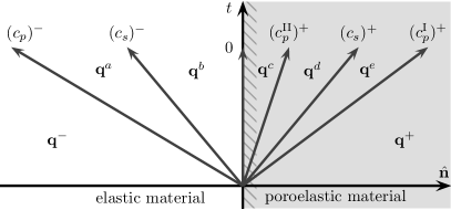
Figure 2: Schematic showing characteristic wave speeds at an elastic/poroelastic interface between two states $\mathbf{q}^{-}$ (elastic) and $\mathbf{q}^{+}$ (poroelastic). $\mathbf{q}^{a}$– $\mathbf{q}^{e}$ denote the intermediate states.

Note that the normal fluid and solid velocities in the poroelastic medium are assumed to be the same as the solid velocity in the elastic medium at the interface. From the Rankine-Hugoniot conditions we obtain

$$\mathbf{q}^{-}-\mathbf{q}^{a} =\beta_{1}^{e}\mathbf{r}_{1}^{e}$$ (144)

$$\mathbf{q}^{a}-\mathbf{q}^{b} =\beta_{2}^{e}\mathbf{r}_{2}^{e}+\beta_{3}^{e}\mathbf{r}_{3}^{e}$$ (145)

$$\mathbf{q}^{c}-\mathbf{q}^{d} =\beta_{10}^{p}\mathbf{r}_{10}^{p}$$ (146)

$$\mathbf{q}^{d}-\mathbf{q}^{e} =\beta_{11}^{p}\mathbf{r}_{11}^{p}+\beta_{12}^{p}\mathbf{r}_{12}^{p}$$ (147)

$$\mathbf{q}^{e}-\mathbf{q}^{-} =\beta_{13}^{p}\mathbf{r}_{13}^{p}$$ (148)

where $\mathbf{r}_{j}^{e}$ is an eigenvector for the elastic domain and $\mathbf{r}_{j}^{p}$ is an eigenvector for the poroelastic domain corresponding to wave speeds $c_{j}^{\pm}$ and hence

$$\mathbf{q}^{-}-\mathbf{q}^{b} =\beta_{1}^{e}\mathbf{r}_{1}^{e}+\beta_{2}^{e}\mathbf{r}_{2}^{e}$$ (149)

$$\mathbf{q}^{c}-\mathbf{q}^{+} =\beta_{10}^{p}\mathbf{r}_{10}^{p}+\beta_{11}^{p}\mathbf{r}_{11}^{p}+\beta_{12}^{p}\mathbf{r}_{12}^{p}+\beta_{13}^{p}\mathbf{r}_{13}^{p}.$$ (150)

Using (137), (140) and (141) we obtain

$$(c_{p}^{e})^{-}\beta_{1}^{e}-(c_{p}^{\mathrm{II}})^{+}\beta_{10}^{p}-(c_{p}^{\mathrm{I}})^{+}\beta_{13}^{p} =\hat{\mathbf{n}}\cdot(\mathbf{v}_{\rm e}^{-}-\mathbf{v}_{\rm s}^{+})$$ (151)

$$(\gamma_{2}c_{p}^{\mathrm{II}})^{+}\beta_{10}^{p}+(\gamma_{1}c_{p}^{\mathrm{I}})^{+}\beta_{13}^{p} =\hat{\mathbf{n}}\cdot\mathbf{v}_{\rm f}^{+}$$ (152)

$$(2\mu_{\mathrm{e}}^{-}+\lambda_{\mathrm{e}}^{-})\beta_{1}^{e}+(2\mu_{\mathrm{fr}}^{+}+\lambda^{+}+\alpha^{+}M^{+}\gamma_{2}^{+})\beta_{10}+(2\mu_{\mathrm{fr}}^{+}+\lambda^{+}+\alpha^{+}M^{+}\gamma_{1}^{+})\beta_{13} =\hat{\mathbf{n}}^{\mathsf{T}}(\mathbf{S}^{-}-\mathbf{T}^{+})\hat{\mathbf{n}}.$$ (153)

As in the poroelastic case, we invert the coefficient matrix

$$\begin{pmatrix}2\mu_{\mathrm{e}}^{-}+\lambda_{\mathrm{e}}^{-}&2\mu_{\mathrm{fr}}^{+}+\lambda^{+}+\alpha^{+}M^{+}\gamma_{2}^{+}&2\mu_{\mathrm{fr}}^{+}+\lambda^{+}+\alpha^{+}M^{+}\gamma_{1}^{+}\\ (c_{p}^{e})^{-}&-(c_{p}^{\mathrm{II}})^{+}&-(c_{p}^{\mathrm{I}})^{+}\\ 0&(\gamma_{2}c_{p}^{\mathrm{II}})^{+}&(\gamma_{1}c_{p}^{\mathrm{I}})^{+}\end{pmatrix}$$

to solve for $\beta_{1}^{e}$, $\beta_{10}^{p}$ and $\beta_{13}^{p}$ and obtain coefficients $\tilde{d}_{ij}$ such that

$$\beta_{1}^{e} =\tilde{d}_{11}\hat{\mathbf{n}}^{\mathsf{T}}(\mathbf{S}^{-}-\mathbf{T}^{+})\hat{\mathbf{n}}+\tilde{d}_{12}\hat{\mathbf{n}}\cdot(\mathbf{v}_{\rm e}^{-}-\mathbf{v}_{\rm s}^{+})\ +\tilde{d}_{13}\hat{\mathbf{n}}\cdot\mathbf{v}_{\rm f}^{+}$$ (154)

$$\beta_{10}^{p} =\tilde{d}_{21}\hat{\mathbf{n}}^{\mathsf{T}}(\mathbf{S}^{-}-\mathbf{T}^{+})\hat{\mathbf{n}}+\tilde{d}_{22}\hat{\mathbf{n}}\cdot(\mathbf{v}_{\rm e}^{-}-\mathbf{v}_{\rm s}^{+})\ +\tilde{d}_{23}\hat{\mathbf{n}}\cdot\mathbf{v}_{\rm f}^{+}$$ (155)

$$\beta_{13}^{p} =\tilde{d}_{31}\hat{\mathbf{n}}^{\mathsf{T}}(\mathbf{S}^{-}-\mathbf{T}^{+})\hat{\mathbf{n}}+\tilde{d}_{32}\hat{\mathbf{n}}\cdot(\mathbf{v}_{\rm e}^{-}-\mathbf{v}_{\rm s}^{+})\ +\tilde{d}_{33}\hat{\mathbf{n}}\cdot\mathbf{v}_{\rm f}^{+}.$$ (156)

Finally, we deal with the shear waves. Using (138) and (142) we obtain

$$\mu_{\mathrm{e}}\beta_{2}^{e}+\mu_{\mathrm{fr}}^{p}\beta_{12}^{p} =\hat{\mathbf{s}}^{\mathsf{T}}(\mathbf{S}^{-}-\mathbf{T}^{+})\hat{\mathbf{n}}$$ (157)

$$(c_{s}^{e})^{-}\beta_{2}^{e}-(c_{s}^{p})^{+}\beta_{12}^{p} =\hat{\mathbf{s}}\cdot(\mathbf{v}_{\rm e}^{-}-\mathbf{v}_{\rm s}^{+}).$$ (158)

Therefore,

$$\beta_{2}^{e} =\frac{(c_{s}^{p})^{+}\hat{\mathbf{s}}^{\mathsf{T}}(\mathbf{S}^{-}-\mathbf{T}^{+})\hat{\mathbf{n}}+\mu_{\mathrm{fr}}^{+}\hat{\mathbf{s}}\cdot(\mathbf{v}_{\rm e}^{-}-\mathbf{v}_{\rm f}^{+})}{(c_{s}^{p})^{+}(\mu_{\mathrm{e}})^{-}+(c_{s}^{e})^{-}(\mu_{\mathrm{fr}})^{+}}$$ (159)

$$\beta_{12}^{p} =\frac{(c_{s}^{e})^{-}\hat{\mathbf{s}}^{\mathsf{T}}(\mathbf{S}^{-}-\mathbf{T}^{+})\hat{\mathbf{n}}-\mu_{\mathrm{e}}^{-}\hat{\mathbf{s}}\cdot(\mathbf{v}_{\rm e}^{-}-\mathbf{v}_{\rm s}^{+})}{(c_{s}^{p})^{+}(\mu_{\mathrm{e}})^{-}+(c_{s}^{e})^{-}(\mu_{\mathrm{fr}})^{+}}.$$ (160)

Similarly we obtain

$$\beta_{3}^{e} =\frac{(c_{s}^{p})^{+}\hat{\mathbf{t}}^{\mathsf{T}}(\mathbf{S}^{-}-\mathbf{T}^{+})\hat{\mathbf{n}}+\mu_{\mathrm{fr}}^{+}\hat{\mathbf{t}}\cdot(\mathbf{v}_{\rm e}^{-}-\mathbf{v}_{\rm f}^{+})}{(c_{s}^{p})^{+}(\mu_{\mathrm{e}})^{-}+(c_{s}^{e})^{-}(\mu_{\mathrm{fr}})^{+}}$$ (161)

$$\beta_{11}^{p} =\frac{(c_{s}^{e})^{-}\hat{\mathbf{t}}^{\mathsf{T}}(\mathbf{S}^{-}-\mathbf{T}^{+})\hat{\mathbf{n}}-\mu_{\mathrm{e}}^{-}\hat{\mathbf{t}}\cdot(\mathbf{v}_{\rm e}^{-}-\mathbf{v}_{\rm s}^{+})}{(c_{s}^{p})^{+}(\mu_{\mathrm{e}})^{-}+(c_{s}^{e})^{-}(\mu_{\mathrm{fr}})^{+}}.$$ (162)

5.2 Upwind numerical flux

For the interface element on the elastic domain, we define an upwind numerical flux $(\Pi\mathbf{q})^{*}$ along $\hat{\mathbf{n}}$ by

$$(\Pi\mathbf{q}^{e})^{*}=\Pi^{-}\mathbf{q}^{-}+Q^{-}(\beta_{1}^{e}(c_{p}^{e})^{-}\mathbf{r}_{1}^{-}+\beta_{2}^{e}(c_{s}^{e})^{-}\mathbf{r}_{2}^{-}+\beta_{3}^{e}(c_{s}^{e})^{-}\mathbf{r}_{3}^{-})$$ (163)

while, for the poroelastic domain, we define an upwind numerical flux $(\Pi\mathbf{q})^{*}$ along $\hat{\mathbf{n}}$ by

$$(\Pi\mathbf{q}^{p})^{*}=\Pi^{+}\mathbf{q}^{+}-Q^{+}(\beta_{10}^{p}(c_{p}^{\mathrm{II}})^{+}\mathbf{r}_{10}^{+}+\beta_{11}^{p}(c_{s})^{+}\mathbf{r}_{11}^{+}+\beta_{12}^{p}(c_{s})^{+}\mathbf{r}_{12}^{+}+\beta_{13}^{p}(c_{p}^{\mathrm{I}})^{+}\mathbf{r}_{13}^{+}).$$ (164)

We define

$$[\![\mathbf{S},\mathbf{T}]\!] =\mathbf{S}^{-}\hat{\mathbf{n}}^{-}+\mathbf{T}^{+}\hat{\mathbf{n}}^{+}$$

$$[\![\mathbf{v}_{\rm e},\mathbf{v}_{\rm s}]\!] =\hat{\mathbf{n}}^{-}{}^{\mathsf{T}}\mathbf{v}_{\rm e}^{-}+\hat{\mathbf{n}}^{+}{}^{\mathsf{T}}\mathbf{v}_{\rm s}^{+}$$

$$[\![\mathbf{v}_{\rm f}]\!] =\hat{\mathbf{n}}^{+}{}^{\mathsf{T}}\mathbf{v}_{\rm f}^{+}$$

$$[\mathbf{v}_{\rm e},\mathbf{v}_{\rm s}] =\mathbf{v}_{\rm e}^{-}-\mathbf{v}_{\rm s}^{+}$$

We now assemble the flux terms for the elastic element:

$$\beta_{1}^{e}(c_{p}^{e})^{-}\mathbf{r}_{1}^{-,e}+\beta_{2}c_{s}^{-}\mathbf{r}_{2}^{-}+\beta_{3}c_{s}^{-}\mathbf{r}_{3}^{-}=\\ (c_{p}^{e})^{-}(d_{11}\hat{\mathbf{n}}^{\mathsf{T}}[\![\mathbf{S},\mathbf{T}]\!]+d_{12}[\![\mathbf{v}_{\rm e},\mathbf{v}_{\rm s}]\!]+d_{13}[\![\mathbf{v}_{\rm f}]\!])\times\begin{pmatrix}\overline{\hat{\mathbf{n}}\otimes\hat{\mathbf{n}}}\\ (c_{p})^{-}\hat{\mathbf{n}}\end{pmatrix}\\ -\frac{(c_{s}^{e})^{-}(c_{s})^{+}}{(c_{s})^{+}(\mu_{\mathrm{e}})^{-}+(c_{s}^{e})^{-}(\mu_{\mathrm{fr}})^{+}}\begin{pmatrix}\overline{\operatorname{sym}(\hat{\mathbf{n}}\otimes(\hat{\mathbf{n}}\times(\hat{\mathbf{n}}\times[\![\mathbf{S},\mathbf{T}]\!])))}\\ (c_{s})^{-}\hat{\mathbf{n}}\times(\hat{\mathbf{n}}\times[\![\mathbf{S},\mathbf{T}]\!])\end{pmatrix}\\ -\frac{(c_{s}^{e})^{-}(\mu_{\mathrm{fr}})^{+}}{(c_{s})^{+}(\mu_{\mathrm{e}})^{-}+(c_{s})^{-}(\mu_{\mathrm{fr}})^{+}}\begin{pmatrix}\overline{\operatorname{sym}(\hat{\mathbf{n}}\otimes(\hat{\mathbf{n}}\times(\hat{\mathbf{n}}\times[\mathbf{v}_{\rm e},\mathbf{v}_{\rm s}])))}\\ (c_{s})^{-}\hat{\mathbf{n}}\times(\hat{\mathbf{n}}\times[\mathbf{v}_{\rm e},\mathbf{v}_{\rm s}])\end{pmatrix}$$ (165)

Finally, we assemble the flux terms for the poroelastic element:

$$\beta_{10}^{p}(c_{p}^{\mathrm{II}})^{+}\mathbf{r}_{10}^{+}+\beta_{11}^{p}(c_{s}^{p})^{+}\mathbf{r}_{11}^{+}+\beta_{12}^{p}(c_{s}^{p})^{+}\mathbf{r}_{12}^{+}+\beta_{13}^{p}(c_{p}^{\mathrm{I}})^{+}\mathbf{r}_{13}^{+}=\\ (c_{p}^{\mathrm{II}})^{+}(\tilde{d}_{21}\hat{\mathbf{n}}^{\mathsf{T}}[\![\mathbf{S},\mathbf{T}]\!]+\tilde{d}_{22}[\![\mathbf{v}_{\rm e},\mathbf{v}_{\rm s}]\!]+\tilde{d}_{23}[\![\mathbf{v}_{\rm f}]\!])\begin{pmatrix}\overline{\hat{\mathbf{n}}\otimes\hat{\mathbf{n}}}\\ -\gamma_{2}^{+}\\ -(c_{p}^{\mathrm{II}})^{+}\hat{\mathbf{n}}\\ -\gamma_{2}^{+}(c_{p}^{\mathrm{II}})^{+}\hat{\mathbf{n}}\end{pmatrix}\\ \frac{-1}{(c_{s}^{p})^{+}(\mu_{\mathrm{e}})^{-}+(c_{s}^{e})^{-}(\mu_{\mathrm{fr}})^{+}}\times\left\{(c_{s}^{e})^{-}(c_{s}^{p})^{+}\begin{pmatrix}\overline{\operatorname{sym}(\hat{\mathbf{n}}\otimes(\hat{\mathbf{n}}\times(\hat{\mathbf{n}}\times[\![\mathbf{S},\mathbf{T}]\!])))}\\ 0\\ -(c_{s})^{-}\hat{\mathbf{n}}\times(\hat{\mathbf{n}}\times[\![\mathbf{S},\mathbf{T}]\!])\\ \frac{(c_{s})^{-}\rho_{f}^{-}}{m^{-}}\hat{\mathbf{n}}\times(\hat{\mathbf{n}}\times[\![\mathbf{S},\mathbf{T}]\!])\end{pmatrix}\right.\\ \left.-\mu_{\mathrm{e}}^{-}(c_{s}^{p})^{+}\begin{pmatrix}\overline{\operatorname{sym}(\hat{\mathbf{n}}\otimes(\hat{\mathbf{n}}\times(\hat{\mathbf{n}}\times[\mathbf{v}_{\rm e},\mathbf{v}_{\rm s}])))}\\ 0\\ -(c_{s})^{-}\hat{\mathbf{n}}\times(\hat{\mathbf{n}}\times[\mathbf{v}_{\rm e},\mathbf{v}_{\rm s}])\\ \frac{(c_{s})^{-}\rho_{f}^{-}}{m^{-}}\hat{\mathbf{n}}\times(\hat{\mathbf{n}}\times[\mathbf{v}_{\rm e},\mathbf{v}_{\rm s}])\end{pmatrix}\right\}.\\ (c_{p}^{\mathrm{I}})^{+}(\tilde{d}_{31}\hat{\mathbf{n}}^{\mathsf{T}}[\![\mathbf{S},\mathbf{T}]\!]+\tilde{d}_{32}[\![\mathbf{v}_{\rm e},\mathbf{v}_{\rm s}]\!]+\tilde{d}_{33}[\![\mathbf{v}_{\rm f}]\!])\times\begin{pmatrix}\overline{\hat{\mathbf{n}}\otimes\hat{\mathbf{n}}}\\ -\gamma_{1}^{+}\\ -(c_{p}^{\mathrm{I}})^{+}\hat{\mathbf{n}}\\ -\gamma_{1}^{+}(c_{p}^{\mathrm{I}})^{+}\hat{\mathbf{n}}\end{pmatrix}$$ (166)

6 Adjoint method

In applications to inverse problems, we wish to quantify a model’s fit to observed data. In seismic problems data normally consists of ground motion measurements following a seismic event due to a passive or active source. Here we are interested in fitting full waveform ground acceleration or velocity data, which requires simulating a forward model many times. Poroelastic wave inverse problems are particularly challenging since most nontrivial problems require multiparameter estimation and the computational cost of the forward problem is expensive and often prohibitive [19, 20]. In both frequentist and Bayesian approaches to inverse problems, a least squares estimate is a good starting point to solving an inverse problem. This requires the solution of a PDE-constrained optimisation problem.

We introduce the following notation

$$L(\mathbf{q})=Q\frac{\partial\mathbf{q}}{\partial t}+\frac{\partial}{\partial x_{i}}(A^{i}\mathbf{q})$$ (167)

where $\mathbf{q}=(\epsilon_{11},\epsilon_{22},\epsilon_{33},\epsilon_{12},\epsilon_{23},\epsilon_{13},\zeta,u_{\rm s},v_{\rm s},w_{\rm s},u_{\rm f},v_{\rm f},w_{\rm f})^{\mathsf{T}}$ and we assume the Einstein summation convention over repeated indices. We consider the hyperbolic system $L(\mathbf{q})=\mathbf{g}+\mathbf{g}_{V}$.

Given time-varying data $\mathbf{d}(x_{r},t)$ define the misfit functional

$$\chi(\bm{\theta})=\frac{1}{2}\sum_{i\in\mathcal{I},r\in\mathcal{R}}\int_{0}^{T}\int_{\Omega}[q_{i}(\bm{\theta},x,t)-d_{i}(x_{r},t)]^{2}\delta(x-x_{r})dxdt$$ (168)

where $\mathbf{q}(\bm{\theta},x,t)$ is the forward map evaluated on the parameter set $\bm{\theta}$, $\mathcal{I}$ is an index set over the observed measurements (i.e. which components of $\mathbf{q}$ are measured, usually velocities), and $\mathcal{R}$ is an index set over the receiver locations $x_{r}$. Gradient-based approaches to minimising (168) require estimation of the Jacobian of (168) with respect to the parameter space $\bm{\theta}$ which usually requires many evaluations of the forward map; this is an expensive calculation as noted above. The adjoint method is a standard approach for computing derivatives of a misfit functional in computational seismology which reduces the number of evaluations of the forward map to one together with one evaluation of a dual, or adjoint, map. Fichtner gives an interesting history of the adjoint method in seismology [13]. When the elastic or poroelastic wave equation is written as a second order system in time, the adjoint map is self-adjoint, although time-reversed, which means the forward solver can be used to solve the adjoint problem, and hence estimate the Jacobian of the least squares misfit functional, [27], [13]. With a first order system this is no longer the case, and more care must be taken to both derive and solve an adjoint equation. Since adjoints are not unique being specified relative to an inner product, the actual choice of the inner product turns out to be crucial to obtain an adjoint equation that is physically meaningful. This was considered in [28] for the elastic wave equation.

We therefore replace (168) by

$$\chi(\bm{\theta})=\frac{1}{2}\sum_{i\in\mathcal{I},r\in\mathcal{R}}\int_{0}^{T}\int_{\Omega}[q_{i}(\bm{\theta},x,t)-d_{i}(x,t)]^{2}w_{i}\delta(x-x_{r})dxdt$$ (169)

where $w_{i}$ are positive weights. We can then define an inner product $\langle\cdot,\cdot\rangle_{W}$ and write (169) as

$$\chi(\bm{\theta})=\frac{1}{2}\langle\mathbf{q}-\mathbf{d},(\mathbf{q}-\mathbf{d})\delta(x-x_{r})\chi_{\mathcal{I}}\rangle_{W}$$ (170)

where $\chi_{\mathcal{I}}$ is an indicator function on the measurement set (=1 if $q_{i}$ is measured, otherwise 0) and for simplicity we have assumed just one receiver location. In the following we take $w_{i}=1$ except for $i=4,5,6$ where we set $w_{i}=2$. The reason for this is that we may write $\mathbf{q}$ in block form

$$\mathbf{q}=\left(\begin{array}[]{c}\mathbf{q}_{1}\\ \hline\cr\mathbf{q}_{2}\end{array}\right)$$ (171)

where $\mathbf{q}_{1}$ contains the 7 strain components $\mathbf{q}_{1}=(\epsilon_{11},\epsilon_{22},\epsilon_{33},\epsilon_{12},\epsilon_{23},\epsilon_{13},\zeta)^{\mathsf{T}}$, while $\mathbf{q}_{2}$ contains the 6 velocity components $\mathbf{q}_{2}=(u_{\rm s},v_{\rm s},w_{\rm s},u_{\rm f},v_{\rm f},w_{\rm f})^{\mathsf{T}}$. Note that the first six entries of $\mathbf{q}_{1}$ is a flattened representation of the strain tensor (5), and the natural inner product is given by the double dot product $\colon$, and the off-diagonal (shear) terms are counted twice. Hence the specification of weights above. In practice the inner product $\langle\cdot,\cdot\rangle_{W}$ defined above makes no difference to the estimation problem since ground motion data is measured and not strain data.

In the following derivations we assume, for simplicity, that the source parameters are known. We define the directional derivative

$$D_{\delta\bm{\theta}}\chi(\bm{\theta})=\lim_{h\rightarrow 0}\frac{1}{h}[\chi(\bm{\theta}+h\delta\bm{\theta})-\chi(\bm{\theta})]$$ (172)

Then

$$D_{\delta\bm{\theta}}\chi=\left\langle(\mathbf{q}-\mathbf{d})\delta(x-x_{r})\chi_{\mathcal{I}},D_{\delta\bm{\theta}}\mathbf{q}\right\rangle_{W}$$ (173)

and

$$D_{\delta\bm{\theta}}L(\mathbf{q}) =(D_{\delta\bm{\theta}}Q)\frac{\partial\mathbf{q}}{\partial t}+Q(D_{\delta\bm{\theta}}\frac{\partial\mathbf{q}}{\partial t})+\frac{\partial}{\partial x_{i}}(D_{\delta\bm{\theta}}(A^{i}\mathbf{q}))$$

$$=Q(\delta\bm{\theta})\frac{\partial\mathbf{q}}{\partial t}+Q\frac{\partial}{\partial t}(D_{\delta\bm{\theta}}(\mathbf{q}))+\frac{\partial}{\partial x_{i}}(A^{i}(\delta\bm{\theta})\mathbf{q}+A^{i}D_{\delta\bm{\theta}}(\mathbf{q}))$$

$$=0$$ (174)

We now take the inner product of (6) with a dual vector $\mathbf{q}^{*}$

$$\left\langle\mathbf{q}^{*},Q(\delta\bm{\theta})\frac{\partial\mathbf{q}}{\partial t}+\frac{\partial}{\partial x_{i}}(A^{i}(\delta\bm{\theta})\mathbf{q})\right\rangle_{W}+\left\langle\mathbf{q}^{*},Q\frac{\partial}{\partial t}(D_{\delta\bm{\theta}}(\mathbf{q}))+\frac{\partial}{\partial x_{i}}(A^{i}D_{\delta\bm{\theta}}(\mathbf{q}))\right\rangle_{W}=0$$ (175)

We have

$$Q\frac{\partial}{\partial t}(D_{\delta\bm{\theta}}(\mathbf{q}))+\frac{\partial}{\partial x_{i}}(A^{i}D_{\delta\bm{\theta}}(\mathbf{q}))=L(D_{\delta\bm{\theta}}\mathbf{q})$$ (176)

Using the definition of the adjoint map on the second term in (175) gives

$$\left\langle\mathbf{q}^{*},L_{\delta\bm{\theta}}(\mathbf{q})\right\rangle_{W}+\left\langle L^{*}\mathbf{q}^{*},D_{\delta\bm{\theta}}(\mathbf{q})\right\rangle_{W}=0$$ (177)

where

$$L_{\delta\bm{\theta}}(\mathbf{q})=Q(\delta\bm{\theta})\frac{\partial\mathbf{q}}{\partial t}+\frac{\partial}{\partial x^{i}}(A^{i}(\delta\bm{\theta})\mathbf{q})$$ (178)

Adding (177) to (173) gives

$$D_{\delta\bm{\theta}}\chi =\left\langle(\mathbf{q}-\mathbf{d})\delta(x-x_{r})\chi_{\mathcal{I}},D_{\delta\bm{\theta}}\mathbf{q}\right\rangle_{W}+\left\langle\mathbf{q}^{*},L_{\delta\bm{\theta}}(\mathbf{q})\right\rangle_{W}+\left\langle L^{*}\mathbf{q}^{*},D_{\delta\bm{\theta}}(\mathbf{q})\right\rangle_{W}$$

$$=\left\langle(\mathbf{q}-\mathbf{d})\delta(x-x_{r})\chi_{\mathcal{I}}+L^{*}\mathbf{q}^{*},D_{\delta\bm{\theta}}\mathbf{q}\right\rangle_{W}+\left\langle\mathbf{q}^{*},L_{\delta\bm{\theta}}(\mathbf{q})\right\rangle_{W}$$ (179)

$D_{\delta\bm{\theta}}\mathbf{q}$ is an expensive calculation so we define $\mathbf{q}^{*}$ to be the solution of the adjoint equation defined by

$$L^{*}\mathbf{q}^{*}=-(\mathbf{q}-\mathbf{d})\delta(x-x_{r})\chi_{\mathcal{I}}$$ (180)

with appropriate initial and boundary conditions given in the next section. Therefore, the derivatives of the misfit functional may be calculated by

$$D_{\delta\bm{\theta}}\chi=\left\langle\mathbf{q}^{*},L_{\delta\bm{\theta}}(\mathbf{q})\right\rangle_{W}$$ (181)

6.1 The formal adjoint

We now derive the formal adjoint of $L(\mathbf{q})$ with respect to the inner product $\langle\cdot,\cdot\rangle_{W}$. First we note that

$$\left\langle\mathbf{q}^{*},Q\frac{\partial\mathbf{q}}{\partial t}\right\rangle_{W}=\int_{\Omega}\left(\left.\bigg{(}Q^{*}\mathbf{q}^{*},\mathbf{q}\bigg{)}_{\mathbb{R}^{13}}\right|_{0}^{T}-\int_{0}^{T}\left(Q^{*}\frac{\partial\mathbf{q}^{*}}{\partial t},\mathbf{q}\right)_{\mathbb{R}^{13}}dt\right)dx$$ (182)

where $(\cdot,\cdot)_{\mathbb{R}^{13}}$ is the Euclidean inner product on $\mathbb{R}^{13}$ with weights $w_{i}$ and $Q^{*}$ is the adjoint of $Q$ in the weighted inner product; in this instance, $Q^{*}=Q^{\mathsf{T}}$. Typically in applications we assume that $\mathbf{q}(x,0)=\mathbf{0}$, while the other boundary term vanishes if we assume $\mathbf{q}^{*}(x,T)=\mathbf{0}$, thus the adjoint field $\mathbf{q}^{*}$ satisfies a final value problem. Next we deal with the spatial terms which again are integrated by parts using Gauss’ theorem.

It is convenient to write $\mathbf{q}$ in block form as in (171)

$$\mathbf{q}=\left(\begin{array}[]{c}\mathbf{q}_{1}\\ \hline\cr\mathbf{q}_{2}\end{array}\right)$$

Similarly we write $A^{i}$ in block form

$$A^{i}=\left(\begin{array}[]{c|c}0&A_{2}^{i}\\ \hline\cr A_{1}^{i}&0\\ \end{array}\right)$$ (183)

Then

$$\left\langle\mathbf{q}^{*},\frac{\partial}{\partial x_{i}}(A^{i}\mathbf{q})\right\rangle_{W} =-\left\langle\frac{\partial}{\partial x_{i}}\left(\begin{array}[]{c}\mathbf{q}_{1}^{*}\\ \hline\cr\mathbf{q}_{2}^{*}\end{array}\right),\left(\begin{array}[]{c}A_{2}^{i}\mathbf{q}_{2}\\ \hline\cr A_{1}^{i}\mathbf{q}_{1}\end{array}\right)\right\rangle_{W}+\text{surface terms}$$ (188)

$$=-\left\langle\left(\begin{array}[]{c|c}0&A_{2}^{i,*}\\ \hline\cr A_{1}^{i,*}&0\\ \end{array}\right)\frac{\partial}{\partial x_{i}}\left(\begin{array}[]{c}\mathbf{q}_{1}^{*}\\ \hline\cr\mathbf{q}_{2}^{*}\end{array}\right),\left(\begin{array}[]{c}\mathbf{q}_{1}\\ \hline\cr\mathbf{q}_{2}\end{array}\right)\right\rangle_{W}+\text{surface terms}$$ (195)

where, for $i=1$,

$$A_{1}^{1,*}=-\begin{pmatrix}1&0&0&0&0&0&0\\ 0&0&0&1&0&0&0\\ 0&0&0&0&0&1&0\\ 0&0&0&0&0&0&-1\\ 0&0&0&0&0&0&0\\ 0&0&0&0&0&0&0\\ \end{pmatrix}$$ (196)

and

$$A_{2}^{1,*}=-\begin{pmatrix}2\mu_{\mathrm{fr}}+\lambda&0&0&\alpha M&0&0\\ \lambda&0&0&\alpha M&0&0\\ \lambda&0&0&\alpha M&0&0\\ 0&\mu_{\mathrm{fr}}&0&0&0&0\\ 0&0&0&0&0&0\\ 0&0&\mu_{\mathrm{fr}}&0&0&0\\ -\alpha M&0&0&-M&0&0\\ \end{pmatrix}$$ (197)

We now dispose of the surface terms: we may write the boundary term as

$$\int_{\partial\Omega}q^{*}_{j}(A_{j,k}^{i}q_{k}n_{i})w_{j}dS$$ (198)

We recall that the first 7 elements of $\mathbf{q}$ are the strain components $(\epsilon_{11},\epsilon_{22},\epsilon_{33},\epsilon_{12},\epsilon_{23},\epsilon_{13},\zeta)^{\mathsf{T}}$. Assuming the traction-free boundary condition in section 3.3 it follows that the last 6 components of $A_{j,k}^{i}q_{k}n_{i}$ vanish. As we will see below, the first 7 elements of $q^{*}$ may be identified as the components of the stress tensors ${\bf\mathbf{T}}$ and $\mathbf{T}_{\rm f}$, and so the traction-free condition also implies that the first 6 components of $q^{*}_{j}(A_{j,k}^{i}n_{i})w_{j}$ vanish. In the case of absorbing boundary conditions at artificial boundaries more care needs to be taken with implementation to ensure that the boundary terms above vanish.

In a similar fashion we obtain

$$A^{i,*}=\left(\begin{array}[]{c|c}0&A_{2}^{i,*}\\ \hline\cr A_{1}^{i,*}&0\\ \end{array}\right)$$

for $i=2,3$ where

$$A_{1}^{2,*} =-\begin{pmatrix}0&0&0&1&0&0&0\\ 0&1&0&0&0&0&0\\ 0&0&0&0&1&0&0\\ 0&0&0&0&0&0&0\\ 0&0&0&0&0&0&-1\\ 0&0&0&0&0&0&0\\ \end{pmatrix} A_{2}^{2,*}=-\begin{pmatrix}0&\lambda&0&0&\alpha M&0\\ 0&2\mu_{\mathrm{fr}}+\lambda&0&0&\alpha M&0\\ 0&\lambda&0&0&\alpha M&0\\ \mu_{\mathrm{fr}}&0&0&0&0&0\\ 0&0&\mu_{\mathrm{fr}}&0&0&0\\ 0&0&0&0&0&0\\ 0&-\alpha M&0&0&-M&0\\ \end{pmatrix}$$ (199)

$$A_{1}^{3,*} =-\begin{pmatrix}0&0&0&0&0&1&0\\ 0&0&0&0&1&0&0\\ 0&0&1&0&0&0&0\\ 0&0&0&0&0&0&0\\ 0&0&0&0&0&0&0\\ 0&0&0&0&0&0&-1\\ \end{pmatrix} A_{2}^{3,*}=-\begin{pmatrix}0&0&\lambda&0&0&\alpha M\\ 0&0&\lambda&0&0&\alpha M\\ 0&0&2\mu_{\mathrm{fr}}+\lambda&0&0&\alpha M\\ 0&0&0&0&0&0\\ 0&\mu_{\mathrm{fr}}&0&0&0&0\\ \mu_{\mathrm{fr}}&0&0&0&0&0\\ 0&0&-\alpha M&0&0&-M\\ \end{pmatrix}$$ (200)

This gives

$$L^{*}\mathbf{q}^{*}=-Q^{*}\frac{\partial\mathbf{q}^{*}}{\partial t}-A^{i,*}\frac{\partial\mathbf{q}}{\partial x_{i}}$$ (201)

Therefore, under the inner product $\langle\cdot,\cdot\rangle_{W}$ the adjoint or dual map $L^{*}$ of $L$ is simply the non-conservative velocity/stress formulation of the poroelastic wave equation, see [23] for the elastic wave case. This permits straightforward derivation of dual flux conditions for the adjoint equation, as well as giving physical meaning to the adjoint.

6.2 Dual numerical fluxes for the adjoint problem

To derive numerical fluxes we again write $\mathbf{q}$ in block form

$$\mathbf{q}=\left(\begin{array}[]{c}\mathbf{q}_{1}\\ \hline\cr\mathbf{q}_{2}\end{array}\right)$$

where $\mathbf{q}_{1}$ is an element of $\mathbb{R}^{7}$ and $\mathbf{q}_{2}$ of $\mathbb{R}^{6}$. The weighted inner product on $\mathbb{R}^{13}$ naturally decomposes to a weighted inner product on $\mathbb{R}^{7}$ and an unweighted inner product on $\mathbb{R}^{6}$. Define a dual vector $\mathbf{q}^{*}$ by setting

$$\left(\begin{array}[]{c}\mathbf{q}_{1}^{*}\\ \hline\cr\mathbf{q}_{2}^{*}\end{array}\right)=\left(\begin{array}[]{c}C\mathbf{q}_{1}\\ \hline\cr\mathbf{q}_{2}\end{array}\right)$$

where

$$C=\begin{pmatrix}2\mu_{\mathrm{fr}}+\lambda&\lambda&\lambda&0&0&0&-\alpha M\\ \lambda&2\mu_{\mathrm{fr}}+\lambda&\lambda&0&0&0&-\alpha M\\ \lambda&\lambda&2\mu_{\mathrm{fr}}+\lambda&0&0&0&-\alpha M\\ 0&0&0&2\mu_{\mathrm{fr}}&0&0&0\\ 0&0&0&0&2\mu_{\mathrm{fr}}&0&0\\ 0&0&0&0&0&2\mu_{\mathrm{fr}}&0\\ -\alpha M&-\alpha M&-\alpha M&0&0&0&M\\ \end{pmatrix}$$ (202)

Note that $C^{*}=C$, i.e. $C$ is self-adjoint in the weighted inner product on $\mathbb{R}^{7}$. Let $D^{k}$ be an element, then (recalling equation (22)) we have

$$\int_{D^{k}}\left(Q_{1}\frac{\partial\mathbf{q}_{1}^{k}}{\partial t}+\frac{\partial}{\partial x_{i}}(A^{i}_{2}\mathbf{q}_{2}^{k}),C\mathbf{p}_{1}\right)_{\mathbb{R}^{7}}+\left(Q_{2}\frac{\partial\mathbf{q}_{2}^{k}}{\partial t}+\frac{\partial}{\partial x_{i}}(A^{i}_{1}\mathbf{q}_{1}^{k}),\mathbf{p}_{2}\right)_{\mathbb{R}^{6}}dx\\ =\int_{D^{k}}\left(Q_{1}\frac{\partial(C\mathbf{q}_{1}^{k})}{\partial t}+C\frac{\partial}{\partial x_{i}}(A^{i}_{2}\mathbf{q}_{2}^{k}),\mathbf{p}_{1}\right)_{\mathbb{R}^{7}}+\left(Q_{2}\frac{\partial\mathbf{q}_{2}^{k}}{\partial t}+\frac{\partial}{\partial x_{i}}(A^{i}_{1}\mathbf{q}_{1}^{k}),\mathbf{p}_{2}\right)_{\mathbb{R}^{6}}dx$$ (203)

Using $CA^{i}_{2}=A_{2}^{i,*}$ and $A_{1}^{i}=A_{1}^{i,*}C$, the following identities are easily derived:

$$C\frac{\partial}{\partial x_{i}}(A^{i}_{2}\mathbf{q}_{2}) =A_{2}^{i,*}\frac{\partial\mathbf{q}_{2}^{*}}{\partial x_{i}}$$ (204)

$$\frac{\partial}{\partial x_{i}}(A_{1}^{i}\mathbf{q}_{1}) =A_{1}^{i,*}\frac{\partial\mathbf{q}_{1}^{*}}{\partial x_{i}}$$ (205)

where for notational convenience we have suppressed the dependency on the element $D^{k}$. This gives

$$\int_{D^{k}}\left(Q_{1}\frac{\partial\mathbf{q}_{1}^{k}}{\partial t}+\frac{\partial}{\partial x_{i}}(A^{i}_{2}\mathbf{q}_{2}^{k}),C\mathbf{p}_{1}\right)_{\mathbb{R}^{7}}+\left(Q_{2}\frac{\partial\mathbf{q}_{2}^{k}}{\partial t}+\frac{\partial}{\partial x_{i}}(A^{i}_{1}\mathbf{q}_{1}^{k}),\mathbf{p}_{2}\right)_{\mathbb{R}^{6}}dx\\ =\int_{D^{k}}\left(Q_{1}\frac{\partial\mathbf{q}_{1}^{*}}{\partial t}+A_{2}^{i,*}\frac{\partial\mathbf{q}_{2}^{*}}{\partial x_{i}},\mathbf{p}_{1}\right)_{\mathbb{R}^{7}}+\left(Q_{2}\frac{\partial\mathbf{q}_{2}^{*}}{\partial t}+A_{1}^{i,*}\frac{\partial\mathbf{q}_{1}^{*}}{\partial x_{i}},\mathbf{p}_{2}\right)_{\mathbb{R}^{6}}dx$$ (206)

This means that a numerical scheme for the forward model automatically gives a scheme for the adjoint model by setting the fluxes as follows:

$$\mathcal{F}^{*}\left(\begin{array}[]{c}\mathbf{q}_{1}^{*}\\ \hline\cr\mathbf{q}_{2}^{*}\end{array}\right)=\mathcal{F}^{*}\left(\begin{array}[]{c}C\mathbf{q}_{1}\\ \hline\cr\mathbf{q}_{2}\end{array}\right)$$ (207)

That is we simply replace $\mathbf{q}_{1}$ by $C\mathbf{q}_{1}$ in the flux terms for the forward model in section (3.5).

We obtain the following upwind flux:

$$\beta_{1}(c_{p}^{\mathrm{I}})^{-}\mathbf{r}_{1}^{-}+\beta_{2}c_{s}^{-}\mathbf{r}_{2}^{-}+\beta_{3}c_{s}^{-}\mathbf{r}_{3}^{-}+\beta_{3}(c_{p}^{\mathrm{II}})^{-}\mathbf{r}_{4}^{-}=\\ (c_{p}^{\mathrm{I}})^{-}(d_{11}\hat{\mathbf{n}}^{\mathsf{T}}[\![\mathbf{T}]\!]+d_{12}\hat{\mathbf{n}}^{\mathsf{T}}[\![\mathbf{T}_{\rm f}]\!]+d_{13}[\![\mathbf{v}_{\rm s}]\!]+d_{14}[\![\mathbf{v}_{\rm f}]\!])\times\begin{pmatrix}\overline{2\mu_{\mathrm{fr}}^{-}\hat{\mathbf{n}}\otimes\hat{\mathbf{n}}+(\lambda^{-}+\alpha^{-}\gamma_{1}^{-}M^{-})I}\\ -(\alpha^{-}+\gamma_{1}^{-})M^{-}\\ (c_{p}^{\mathrm{I}})^{-}\hat{\mathbf{n}}\\ \gamma_{1}^{-}(c_{p}^{\mathrm{I}})^{-}\hat{\mathbf{n}}\end{pmatrix}\\ -\frac{(c_{s})^{-}(c_{s})^{+}}{(c_{s})^{+}(\mu_{\mathrm{fr}})^{-}+(c_{s})^{-}(\mu_{\mathrm{fr}})^{+}}\begin{pmatrix}\overline{2\mu_{\mathrm{fr}}^{-}\operatorname{sym}(\hat{\mathbf{n}}\otimes(\hat{\mathbf{n}}\times(\hat{\mathbf{n}}\times[\![\mathbf{T}]\!])))}\\ 0\\ (c_{s})^{-}\hat{\mathbf{n}}\times(\hat{\mathbf{n}}\times[\![\mathbf{T}]\!])\\ \frac{-(c_{s})^{-}\rho_{f}^{-}}{m^{-}}\hat{\mathbf{n}}\times(\hat{\mathbf{n}}\times[\![\mathbf{T}]\!])\end{pmatrix}\\ -\frac{(c_{s})^{-}(\mu_{\mathrm{fr}})^{+}}{(c_{s})^{+}(\mu_{\mathrm{fr}})^{-}+(c_{s})^{-}(\mu_{\mathrm{fr}})^{+}}\begin{pmatrix}\overline{2\mu_{\mathrm{fr}}^{-}\operatorname{sym}(\hat{\mathbf{n}}\otimes(\hat{\mathbf{n}}\times(\hat{\mathbf{n}}\times[\![\mathbf{v}_{\rm s}]\!])))}\\ 0\\ (c_{s})^{-}\hat{\mathbf{n}}\times(\hat{\mathbf{n}}\times[\mathbf{v}_{\rm s}])\\ \frac{-(c_{s})^{-}\rho_{f}^{-}}{m^{-}}\hat{\mathbf{n}}\times(\hat{\mathbf{n}}\times[\mathbf{v}_{\rm s}])\end{pmatrix}\\ +(c_{p}^{\mathrm{II}})^{-}(d_{21}\hat{\mathbf{n}}^{\mathsf{T}}[\![\mathbf{T}]\!]+d_{22}\hat{\mathbf{n}}^{\mathsf{T}}[\![\mathbf{T}_{\rm f}]\!]+d_{23}[\![\mathbf{v}_{\rm s}]\!]+d_{24}[\![\mathbf{v}_{\rm f}]\!])\times\\ \begin{pmatrix}\overline{2\mu_{\mathrm{fr}}^{-}\hat{\mathbf{n}}\otimes\hat{\mathbf{n}}+(\lambda^{-}+\alpha^{-}\gamma_{2}^{-}M^{-})I}\\ -(\alpha^{-}+\gamma_{2}^{-})M^{-}\\ (c_{p}^{\mathrm{II}})^{-}\hat{\mathbf{n}}\\ \gamma_{2}^{-}(c_{p}^{\mathrm{II}})^{-}\hat{\mathbf{n}}\end{pmatrix}$$ (208)

6.3 Dual numerical fluxes for coupled elastic/poroelastic problems

In a similar manner one can derive dual numerical fluxes for elastic and coupled elastic and poroelastic problems, which we state below for convenience. The elastic case can be found in [29] and is repeated here for completeness and notational consistency.

For the elastic case we have:

$$\beta_{1}(c_{p})^{-}\mathbf{r}_{1}^{-}+\beta_{2}c_{s}^{-}\mathbf{r}_{2}^{-}+\beta_{3}c_{s}^{-}\mathbf{r}_{3}^{-}=\\ \frac{(c_{p})^{-}c_{p}^{+}\hat{\mathbf{n}}^{\mathsf{T}}[\![\mathbf{S}]\!]+(c_{p})^{-}(\lambda_{\mathrm{e}}^{+}+2\mu_{\mathrm{e}}^{+})[\![\mathbf{v}_{\rm e}]\!]}{c_{p}^{+}(\lambda_{\mathrm{e}}^{-}+2\mu_{\mathrm{e}}^{-})+c_{p}^{-}(\lambda_{\mathrm{e}}^{+}+2\mu_{\mathrm{e}}^{+})}\begin{pmatrix}\overline{2\mu_{\mathrm{e}}^{-}\hat{\mathbf{n}}\otimes\hat{\mathbf{n}}+\lambda_{e}^{-}I}\\ (c_{p})^{-}\hat{\mathbf{n}}\end{pmatrix}\\ -\frac{(c_{s})^{-}(c_{s})^{+}}{(c_{s})^{+}(\mu_{\mathrm{e}})^{-}+(c_{s})^{-}(\mu_{\mathrm{e}})^{+}}\begin{pmatrix}\overline{2\mu_{\mathrm{e}}^{-}\operatorname{sym}(\hat{\mathbf{n}}\otimes(\hat{\mathbf{n}}\times(\hat{\mathbf{n}}\times[\![\mathbf{T}]\!])))}\\ (c_{s})^{-}\hat{\mathbf{n}}\times(\hat{\mathbf{n}}\times[\![\mathbf{T}]\!])\end{pmatrix}\\ -\frac{(c_{s})^{-}(\mu_{\mathrm{e}})^{+}}{(c_{s})^{+}(\mu_{\mathrm{e}})^{-}+(c_{s})^{-}(\mu_{\mathrm{e}})^{+}}\begin{pmatrix}\overline{2\mu_{\mathrm{e}}^{-}\operatorname{sym}(\hat{\mathbf{n}}\otimes(\hat{\mathbf{n}}\times(\hat{\mathbf{n}}\times[\![\mathbf{v}_{\rm e}]\!])))}\\ (c_{s})^{-}\hat{\mathbf{n}}\times(\hat{\mathbf{n}}\times[\mathbf{v}_{\rm s}])\end{pmatrix}$$ (209)

For an interface element on the elastic domain we define an upwind flux by:

$$\beta_{1}^{e}(c_{p}^{e})^{-}\mathbf{r}_{1}^{-,e}+\beta_{2}c_{s}^{-}\mathbf{r}_{2}^{-}+\beta_{3}c_{s}^{-}\mathbf{r}_{3}^{-}=\\ (c_{p}^{e})^{-}(d_{11}\hat{\mathbf{n}}^{\mathsf{T}}[\![\mathbf{S},\mathbf{T}]\!]+d_{12}[\![\mathbf{v}_{\rm e},\mathbf{v}_{\rm s}]\!]+d_{13}[\![\mathbf{v}_{\rm f}]\!])\times\begin{pmatrix}\overline{2\mu_{\mathrm{e}}^{-}\hat{\mathbf{n}}\otimes\hat{\mathbf{n}}+\lambda_{\mathrm{e}}^{-}I}\\ (c_{p})^{-}\hat{\mathbf{n}}\end{pmatrix}\\ -\frac{(c_{s}^{e})^{-}(c_{s})^{+}}{(c_{s})^{+}(\mu_{\mathrm{e}})^{-}+(c_{s}^{e})^{-}(\mu_{\mathrm{fr}})^{+}}\begin{pmatrix}\overline{2\mu_{\mathrm{e}}^{-}\operatorname{sym}(\hat{\mathbf{n}}\otimes(\hat{\mathbf{n}}\times(\hat{\mathbf{n}}\times[\![\mathbf{S},\mathbf{T}]\!])))}\\ (c_{s})^{-}\hat{\mathbf{n}}\times(\hat{\mathbf{n}}\times[\![\mathbf{S},\mathbf{T}]\!])\end{pmatrix}\\ -\frac{(c_{s}^{e})^{-}(\mu_{\mathrm{fr}})^{+}}{(c_{s})^{+}(\mu_{\mathrm{e}})^{-}+(c_{s})^{-}(\mu_{\mathrm{fr}})^{+}}\begin{pmatrix}\overline{2\mu_{\mathrm{e}}^{-}\operatorname{sym}(\hat{\mathbf{n}}\otimes(\hat{\mathbf{n}}\times(\hat{\mathbf{n}}\times[\mathbf{v}_{\rm e},\mathbf{v}_{\rm s}])))}\\ (c_{s})^{-}\hat{\mathbf{n}}\times(\hat{\mathbf{n}}\times[\mathbf{v}_{\rm e},\mathbf{v}_{\rm s}])\end{pmatrix}$$ (210)

Finally, for an interface element on the poroelastic domain we have

$$\beta_{10}^{p}(c_{p}^{\mathrm{II}})^{+}\mathbf{r}_{10}^{+}+\beta_{11}^{p}(c_{s}^{p})^{+}\mathbf{r}_{11}^{+}+\beta_{12}^{p}(c_{s}^{p})^{+}\mathbf{r}_{12}^{+}+\beta_{13}^{p}(c_{p}^{\mathrm{I}})^{+}\mathbf{r}_{13}^{+}=\\ (c_{p}^{\mathrm{II}})^{+}(\tilde{d}_{21}\hat{\mathbf{n}}^{\mathsf{T}}[\![\mathbf{S},\mathbf{T}]\!]+\tilde{d}_{22}[\![\mathbf{v}_{\rm e},\mathbf{v}_{\rm s}]\!]+\tilde{d}_{23}[\![\mathbf{v}_{\rm f}]\!])\times\begin{pmatrix}\overline{2\mu_{\mathrm{fr}}^{+}\hat{\mathbf{n}}\otimes\hat{\mathbf{n}}+(\lambda^{+}+\alpha^{+}\gamma_{2}^{+}M^{+})I}\\ -(\alpha^{+}+\gamma_{2}^{+})M^{+}\\ -(c_{p}^{\mathrm{II}})^{+}\hat{\mathbf{n}}\\ -\gamma_{2}^{+}(c_{p}^{\mathrm{II}})^{+}\hat{\mathbf{n}}\end{pmatrix}\\ -\frac{1}{(c_{s}^{p})^{+}(\mu_{\mathrm{e}})^{-}+(c_{s}^{e})^{-}(\mu_{\mathrm{fr}})^{+}}\times\left\{(c_{s}^{e})^{-}(c_{s}^{p})^{+}\begin{pmatrix}\overline{2\mu_{\mathrm{fr}}^{+}\operatorname{sym}(\hat{\mathbf{n}}\otimes(\hat{\mathbf{n}}\times(\hat{\mathbf{n}}\times[\![\mathbf{S},\mathbf{T}]\!])))}\\ 0\\ -(c_{s})^{+}\hat{\mathbf{n}}\times(\hat{\mathbf{n}}\times[\![\mathbf{S},\mathbf{T}]\!])\\ \frac{(c_{s})^{+}\rho_{f}^{+}}{m^{+}}\hat{\mathbf{n}}\times(\hat{\mathbf{n}}\times[\![\mathbf{S},\mathbf{T}]\!])\end{pmatrix}\right.\\ \left.-\mu_{\mathrm{e}}^{-}(c_{s}^{p})^{+}\begin{pmatrix}\overline{2\mu_{\mathrm{fr}}^{+}\operatorname{sym}(\hat{\mathbf{n}}\otimes(\hat{\mathbf{n}}\times(\hat{\mathbf{n}}\times[\mathbf{v}_{\rm e},\mathbf{v}_{\rm s}])))}\\ 0\\ -(c_{s})^{+}\hat{\mathbf{n}}\times(\hat{\mathbf{n}}\times[\mathbf{v}_{\rm e},\mathbf{v}_{\rm s}])\\ \frac{(c_{s})^{+}\rho_{f}^{+}}{m^{+}}\hat{\mathbf{n}}\times(\hat{\mathbf{n}}\times[\mathbf{v}_{\rm e},\mathbf{v}_{\rm s}])\end{pmatrix}\right\}\\ +(c_{p}^{\mathrm{I}})^{+}(\tilde{d}_{31}\hat{\mathbf{n}}^{\mathsf{T}}[\![\mathbf{S},\mathbf{T}]\!]+\tilde{d}_{32}[\![\mathbf{v}_{\rm e},\mathbf{v}_{\rm s}]\!]+\tilde{d}_{33}[\![\mathbf{v}_{\rm f}]\!])\times\begin{pmatrix}\overline{2\mu_{\mathrm{fr}}^{+}\hat{\mathbf{n}}\otimes\hat{\mathbf{n}}+(\lambda^{+}+\alpha^{+}\gamma_{1}^{+}M^{+})I}\\ -(\alpha^{+}+\gamma_{1}^{+})M^{+}\\ -(c_{p}^{\mathrm{I}})^{+}\hat{\mathbf{n}}\\ -\gamma_{1}^{+}(c_{p}^{\mathrm{I}})^{+}\hat{\mathbf{n}}\end{pmatrix}$$ (211)

6.4 Discussion

6.4.1 Implementation

It turns out that implementation of the adjoint method to estimating derivatives of an objective functional is quite straightforward as we now show. Once again it is convenient to write $\mathbf{q}$ and $\mathbf{q}^{*}$ in block form:

$$\mathbf{q}=\left(\begin{array}[]{c}\mathbf{q}_{1}\\ \hline\cr\mathbf{q}_{2}\end{array}\right),\quad\mathbf{q}^{*}=\left(\begin{array}[]{c}\mathbf{q}_{1}^{*}\\ \hline\cr\mathbf{q}_{2}^{*}\end{array}\right)$$

Then

$$L_{\delta\theta}(\mathbf{q}) =\left(\begin{array}[]{c|c}I&0\\ \hline\cr 0&Q_{2}(\delta\theta)\\ \end{array}\right)\frac{\partial}{\partial t}\left(\begin{array}[]{c}\mathbf{q}_{1}\\ \hline\cr\mathbf{q}_{2}\end{array}\right)+\frac{\partial}{\partial x}\left(\begin{array}[]{c|c}0&A_{2}^{i}\\ \hline\cr A_{1}^{i}(\delta\theta)&0\\ \end{array}\right)\left(\begin{array}[]{c}\mathbf{q}_{1}\\ \hline\cr\mathbf{q}_{2}\end{array}\right)$$ (220)

$$=Q_{2}(\delta\theta)\frac{\partial\mathbf{q}_{2}}{\partial t}+\frac{\partial}{\partial x}(A_{1}^{i}(\delta\theta)\mathbf{q}_{1})$$ (221)

since from equation (21) we have

$$\frac{\partial\mathbf{q}_{1}}{\partial t}+\frac{\partial}{\partial x}(A_{2}^{i}\mathbf{q}_{2})=0$$

This means that (181) reduces to computing

$$D_{\delta\bm{\theta}}\chi=\left\langle\mathbf{q}_{2}^{*},L_{\delta\bm{\theta}}^{2}(\mathbf{q})\right\rangle_{W_{2}}$$ (222)

where

$$L_{\delta\bm{\theta}}^{2}(\mathbf{q})=Q_{2}(\delta\theta)\frac{\partial\mathbf{q}_{2}}{\partial t}+\frac{\partial}{\partial x}(A_{2}^{i}(\delta\theta)\mathbf{q}_{1})$$

and $W_{2}$ is the restriction of $W$ to $\mathbf{q}_{2}$, the velocity components of $\mathbf{q}$. This means that to compute $D_{\delta\bm{\theta}}\chi$ we only need the velocity components $\mathbf{q}_{2}$ and $\mathbf{q}_{2}^{*}$ of $\mathbf{q}$ and $\mathbf{q}^{*}$. Thus for implementation it is immaterial whether we use a conservative velocity/strain or non-conservative velocity/stress (adjoint) formulation to compute $\mathbf{q}^{*}$ since we only need $\mathbf{q}^{*}_{2}$.

6.4.2 Time reversal

Implementation of a time-reversed adjoint solver needs some care since the downwind fluxes given above are with respect to forward time integration. Integrating backwards from the final time $t=T$ to $t=0$ they become upwind fluxes and result in a divergent scheme. To obtain a downwind scheme one simply has to map the wavespeeds $c\rightarrow-c$.

6.4.3 Fréchet kernels of poroelastic parameters

Sensitivity or Fréchet kernels obtained from (181) by taking the integral with respect to time are a useful tool in computational seismology; we refer to [13], Chapter 9, and [27] for the elastic case. Due to the nonlinear relationships between the constitutive parameters in the Hooke’s laws (8)-(9) and the physical parameters in equation (10)-(12), Fréchet kernels corresponding to the primary physical constants like porosity would be unwieldy. Therefore, in the following, we use the derived model parameters $\rho_{\mathrm{a}},\rho_{\mathrm{f}}$ and $m$ for densities, $\kappa_{\mathrm{fr}}$ and $\mu_{\mathrm{fr}}$ for stiffness parameters and $\alpha$ and $M$ for coupling parameters.

For the density parameters we obtain kernels $k_{\rho_{\mathrm{a}}}$, $k_{\rho_{\mathrm{f}}}$ and $k_{m}$ given by

$$k_{\rho_{\mathrm{a}}} =\int_{0}^{T}\left(\mathbf{u}^{*},\frac{\partial\mathbf{u}}{\partial t}\right)_{\mathbb{R}^{3}}dt$$ (223)

$$k_{\rho_{\mathrm{f}}} =\int_{0}^{T}\left(\mathbf{u}^{*},\frac{\partial\mathbf{u}_{\rm f}}{\partial t}\right)_{\mathbb{R}^{3}}+\left(\mathbf{u}_{\rm f}^{*},\frac{\partial\mathbf{u}}{\partial t}\right)_{\mathbb{R}^{3}}dt$$ (224)

$$k_{m} =\int_{0}^{T}\left(\mathbf{u}_{\rm f}^{*},\frac{\partial\mathbf{u}_{\rm f}}{\partial t}\right)_{\mathbb{R}^{3}}dt\$$ (225)

For the stiffness parameters we obtain kernels $k_{\kappa_{\mathrm{fr}}}$ and $k_{\mu_{\mathrm{fr}}}$ where

$$k_{\kappa_{\mathrm{fr}}} =-\int_{0}^{T}\left(\mathbf{u}^{*},\nabla\operatorname{trace}(E)\right)_{\mathbb{R}^{3}}dt$$ (226)

$$k_{\mu_{\mathrm{fr}}} =-\int_{0}^{T}\left(\mathbf{u}^{*},\nabla\cdot E-\frac{1}{3}\nabla\operatorname{trace}(E)\right)_{\mathbb{R}^{3}}dt$$ (227)

For the coupling coefficients we first define an auxiliary kernel $k_{\alpha,M}$ by

$$k_{\alpha,M}=\int_{0}^{T}\left(\mathbf{u},\nabla\zeta\right)_{\mathbb{R}^{3}}-\left(\mathbf{u}_{\rm f},\nabla\operatorname{trace}(E)\right)_{\mathbb{R}^{3}}dt$$ (228)

This gives kernels $k_{\alpha}$ and $k_{M}$ defined by

$$k_{\alpha} =Mk_{\alpha,M}$$ (229)

$$k_{M} =\alpha k_{\alpha,M}+\int_{0}^{T}\left(\mathbf{u}_{\rm f},\nabla\zeta\right)_{\mathbb{R}^{3}}dt$$ (230)

We may then write

$$D_{\delta\bm{\theta}}\chi=\int_{\Omega}(\delta\rho_{\mathrm{a}})k_{\rho_{\mathrm{a}}}+(\delta\rho_{\mathrm{f}})k_{\rho_{\mathrm{f}}}+(\delta m)k_{m}+(\delta\kappa_{\mathrm{fr}})k_{\kappa_{\mathrm{fr}}}+(\delta\mu_{\mathrm{fr}})k_{\mu_{\mathrm{fr}}}+(\delta\alpha)k_{\alpha}+(\delta M)k_{M}dx$$ (231)

7 Numerical experiments

In this section, we consider several numerical experiments. First, we consider the convergence properties of the numerical scheme in the inviscid and low- and high-frequency viscous regimes; we verify that, except in some cases of very small permeability, our code approaches the optimal convergence behaviour of the DG method (see discussion in [15, Chapter 4] and references therein). We then give an example of heterogeneous poroelastic material to show that our code naturally handles material discontinuities, a necessary feature in applications to groundwater tomography. Finally we give an example of the adjoint method.

In the simulations described below, the length of the time step $\Delta t$ is computed from

$$\Delta t=C\frac{h_{\min}}{c_{\max}p^{2}}$$ (232)

where $C$ is a constant, $c_{\max}$ is the maximum wave speed over all elements, $p$ is the basis order and $h_{\min}$ is the smallest distance between two vertices in any element. In the simulations, we set $C=0.4$ unless otherwise stated.

7.1 Convergence analysis

Convergence tests were carried out on a cubical domain $\Omega=[0,5]\times[0,5]\times[0,5]$ m with four regular grids of different side lengths (formed by dividing the domain into subcubes and dividing each subcube into tetrahedra) and inhomogeneous Dirichlet boundary conditions. For time-stepping, in this section we used the five-stage, fourth-order accurate low-storage explicit Runge-Kutta (LSERK) method originated in [9] and used in [15]. With three-dimensional meshes, the advantages of low-storage methods, storing fewer intermediate results than general Runge-Kutta methods, become particularly apparent.

The material parameters are given in Table 3. We consider three cases. In the first case we consider wave propagation in an inviscid setting, while the other two involve viscous flow in Biot’s low- and high-frequency settings respectively. In Table 4, we list the assumed frequencies, viscosities, permeabilities, and the derived wave velocities. The frequency was set at 2,000 Hz so that the test domain captured around three wavelengths of the fast P-wave. Note that with the high-frequency case we also need to define the quality factor (see Section 4.2).

Analytic plane wave solutions consisting of fast and slow P-waves and S-waves were constructed from plane wave solutions of the form

$$\mathbf{q}=\mathbf{q}_{0}e^{\mathrm{i}(k_{x}x+k_{y}y+k_{z}z-\omega t)}$$

where $\mathrm{i}=\sqrt{-1}$, $\omega$ is an angular frequency, and $k_{x}$, $k_{y}$ and $k_{z}$ are complex wave numbers in the $x$-, $y$- and $z$-directions, respectively. In the inviscid case, we consider dissipating waves of the form

$$\mathbf{q}=\operatorname{Re}\left(\sum_{j=1}^{13}\alpha_{j}\mathbf{r}_{j}e^{\mathrm{i}(k_{x,j}+k_{y,j}+k_{z,j}-\omega t)}\right)$$

where $\mathbf{r}_{j}$ is an eigenvector of the $13\times 13$ matrix

$$\Pi=Q^{-1}(\hat{n}_{x}A^{1}+\hat{n}_{y}A^{2}+\hat{n}_{z}A^{3})$$

where $n_{x}$, $n_{y}$ and $n_{z}$ are direction cosines. In the reported examples, we set $[k_{x},k_{y},k_{z}]$ to be a vector parallel to $[0.9,1.0,1.1]$, so as not to align with the geometry of the regular grid in use. For the viscous low- and high-frequency cases the wave speeds and dissipation are frequency-dependent.

Table 3: Material parameters used in the convergence analysis.

variable name	symbol
solid density	$\rho_{\mathrm{s}}$ (kg/m3)	2650
fluid density	$\rho_{\mathrm{f}}$ (kg/m3)	900
fluid bulk modulus	$\kappa_{\mathrm{f}}$ (GPa)	2.0
frame bulk modulus	$\kappa_{\mathrm{fr}}$ (GPa)	10.0
solid bulk modulus	$\kappa_{\mathrm{s}}$ (GPa)	12.0
frame shear modulus	$\mu_{\mathrm{fr}}$ (GPa)	5.0
tortuosity	$\tau$	1.2
porosity	$\phi$	0.3

Table 4: This table lists the plane wave frequency $f_{0}$, viscosity $\eta$, permeability $k$, quality factor $Q_{0}$, Biot’s characteristic frequency $f_{c}$, and wave velocities $(c_{p}^{\mathrm{I}},c_{p}^{\mathrm{II}},c_{s})$ for the three cases studied.

case	$f_{0}$ (Hz)	$\eta$ (Pa$\cdot$s)	$k$ (m2)	$Q_{0}$	$f_{c}$ (Hz)	$c_{p}^{\mathrm{I}}$ (m/s)	$c_{p}^{\mathrm{II}}$ (m/s)	$c_{s}$ (m/s)
inviscid	2000	0	-	-	-	2967	1411	1622
low-frequency	2000	0.001	10-12	-	44209.71	2817	414	1534
high-frequency	2000	0.001	10-8	30	4.42	2967	1411	1622

The numerical solver was initialised with the analytic plane wave solution at time $t=0$, and the boundary values were set with the values of the analytic plane wave. The tests were carried out using plane waves with a fixed frequency $f_{0}$ (see Table 4). The total simulation time was taken to be $1/f_{0}$. The analytic and numerical solutions were compared at the final simulation time over the whole computational domain $\Omega$ by, on each element $D^{k}$, interpolating a polynomial of degree at most $p$ through the exact solution values, calculating the distance in $L^{2}(D^{k})$ between this polynomial and the polynomial representing the simulated solution, and combining the results over all elements to give a distance in $L^{2}(\Omega)$. Errors are reported only for the solid velocity component $u_{\rm s}$ in all cases.

The convergence rate is defined by

$$\mbox{rate}=\log{\left(\frac{\|e^{\ell}\|_{2}}{\|e^{\ell-1}\|_{2}}\right)}\bigg{/}\log{\left(\frac{h_{\min}^{\ell}}{h_{\min}^{\ell-1}}\right)}$$ (233)

where $\|e^{\ell}\|_{2}$ is the $L^{2}$ norm of the error $e^{\ell}$ as described above and $h_{\min}^{\ell}$ is the minimal distance between adjacent vertices in the $\ell$’th mesh; here the meshes are ordered in decreasing order of $h_{\min}$.

Table 5 shows the convergence rate for the inviscid, viscous (low-frequency), and viscous (high-frequency) cases. The results shows that the method is consistent with the optimal $p+1$, for order $p$.

Table 5: The convergence rate as a function of the grid parameter $h_{\min}$ for three basis orders starting from order 3 (top), order 5 (middle), and ending with order 6 (bottom). Convergence rates together with the $L^{2}$-error values are reported for the inviscid (columns 2 and 3), viscous (low-frequency, columns 4 and 5), and viscous (high-frequency, columns 6 and 7) cases.

	inviscid		low-frequency		high-frequency
$h_{\min}$ (m)	$L^{2}$ error	rate	$L^{2}$ error	rate	$L^{2}$ error	rate
0.3125	2.032e-01	—	2.020e-01	—	1.986e-01	—
0.2632	1.051e-01	3.8362	1.046e-01	3.8301	1.031e-01	3.8157
0.2083	4.059e-02	4.0728	4.042e-02	4.0695	3.977e-02	4.0780
0.1786	2.186e-02	4.0140	2.171e-02	4.0323	2.144e-02	4.0088
0.3125	6.640e-03	—	7.196e-03	—	6.476e-03	—
0.2632	2.432e-03	5.8448	2.808e-03	5.4762	2.382e-03	5.8206
0.2083	6.415e-04	5.7045	7.130e-04	5.8679	6.283e-04	5.7043
0.1786	2.446e-04	6.2553	2.594e-04	6.5585	2.397e-04	6.2500
0.3125	1.033e-03	—	1.125e-03	—	1.005e-03	—
0.2632	3.233e-04	6.7586	3.835e-04	6.2620	3.151e-04	6.7513
0.2083	6.375e-05	6.9503	8.913e-05	6.2462	6.237e-05	6.9334
0.1786	2.165e-05	7.0072	3.547e-05	5.9780	2.122e-05	6.9944

7.1.1 The low frequency case: very small permeability

As noted in the introduction to Section 4, the accuracy of the low-storage explicit Runge-Kutta (LSERK) scheme falls off as the permeability decreases to zero in the low frequency regime. In this section we give convergence results for an example in which the permeability is $k=10^{-14}$ m², which may be regarded as a fairly extreme test of a time integration scheme. On the meshes and basis orders used for Table 5, the LSERK scheme failed in every case, with all fields rapidly diverging to $\infty$.

For small $k$, stiffness is introduced into the system by the low-frequency dissipation terms $\mathbf{g}$ described by (25); having no space derivatives, these play no role in the spatial semidiscretisation of the system, and appear unchanged in the ODE system, where they are localised on individual nodes. To deal with them, we tried two techniques: operator splitting and an IMEX (implicit-explicit) Runge-Kutta scheme. In both approaches, the idea is to regard the right-hand side of the ODE system as the sum of two terms: the stiff term $\mathbf{g}$ and the remaining, non-stiff, conservation terms.

In a recent paper [26] on the Biot equation in two dimensions, it is observed that the ODE system with only the stiff terms on the right-hand side may be solved explicitly. This remains true in three dimensions: if we compute $Q^{-1}\mathbf{g}$, we find a matrix that is zero outside the lower-right $6\times 6$ block; this block, itself broken down into $3\times 3$ blocks, acts on the velocity terms as follows

$$\begin{bmatrix}\rho_{\mathrm{a}}I&\rho_{\mathrm{f}}I\\ \rho_{\mathrm{f}}I&mI\end{bmatrix}^{-1}\begin{bmatrix}0&0\\ 0&-(\eta/k)I\end{bmatrix}\begin{bmatrix}*\\ *\\ *\\ u_{\rm f}\\ v_{\rm f}\\ w_{\rm f}\end{bmatrix}=\frac{\eta}{(m\rho_{\mathrm{a}}-\rho_{\mathrm{f}}^{2})k}\begin{bmatrix}0&\rho_{\mathrm{f}}I\\ 0&\rho_{\mathrm{a}}I\end{bmatrix}\begin{bmatrix}*\\ *\\ *\\ u_{\rm f}\\ v_{\rm f}\\ w_{\rm f}\end{bmatrix}$$ (234)

Here $0$, $I$ represent the $3\times 3$ zero and identity matrices and asterisks denote terms that are multiplied by zero, so have no part to play.

Diagonalising this triangular matrix is entirely straightforward: its eigenvalues are $0$ and $\rho_{\mathrm{a}}\eta/((m\rho_{\mathrm{a}}-\rho_{\mathrm{f}}^{2})k)$ and its eigenvectors are readily obtained, leading to a simple, explicit solution to the associated ODE system.

We can now follow [26] and implement Godunov splitting [23, Section 17.3]: at each time-step, given an initial value $\mathbf{q}_{n}$ at time $t_{n}$ from the previous timestep, we begin by explicitly finding the solution to the stiff part of the system at the next time-step, $t_{n+1}$; we then feed this back as a new initial value at $t_{n}$ and from that use the LSERK scheme to find an approximate solution to the non-stiff part of the system at $t_{n+1}$. This serves as our approximate solution $\mathbf{q}_{n+1}$ of the whole system at $t_{n+1}$, and we can repeat the process.

This immediately results in a stable scheme, but the errors involved in this splitting method are rather large: first-order in the length of the time step [23, Section 17.3]. In an attempt to mitigate this, we also considered Strang splitting [23, Section 17.4]: instead of a whole time-step of the analytic stiff solution followed by a whole timestep of the LSERK non-stiff solution, this comprises half a time step of analytic stiff, a whole timestep of LSERK non-stiff, and a final half time step of analytic stiff. As in the Godunov splitting, the final values of the system at the end of each (partial) time-step are fed back as initial values to the next (partial) time-step. This has scarcely any more computational cost (compared to an LSERK step, the cost of the analytic solution is vanishingly small), and should improve the time-stepping error to second-order accuracy [23, Section 17.4].

Table 6 shows the errors and convergence rates for a few examples, using time-steps $\Delta t$ and $\Delta t/16$ (intermediate $\Delta t/2^{n}$ results were calculated but are not presented here). As expected, Strang splitting gives better results than Godunov splitting (although the difference is not huge; it is noted in [23, Section 17.5] that this is not uncommon). Both methods give noticeably better results when the time-step length is decreased; this is in marked contrast to the non-stiff results in Table 5, which remain unchanged to four or more decimal places when the time-step is halved. This suggests that, in Table 5, we are seeing almost entirely spatial discretisation errors, with little contribution from time discretisation, whereas in Table 6, time discretisation is still making a noticeable contribution to the error, even at 16 times the base number of steps. At order $3$, we can approach the optimal convergence rate of $4$, but only by significantly reducing the time-step. At order $5$, even reducing the time-step by a factor of $16$ does not give anything close to the optimal rate, but even so we do see the errors being greatly reduced. In summary, the splitting methods are an effective, but possibly sub-optimal and certainly costly, way of addressing the stiffness caused by very small permeability.

Table 6: Convergence rates for the stiff case, using Godunov splitting (top) and Strang splitting (bottom), with three meshes and time steps $\Delta t$ and $\Delta t/16$. Again, only the solid velocity component $u_{\rm s}$ is reported. Some values are highlighted for comparison with Table 7.

	Order 3				Order 5
	Time step / 1		Time step / 16		Time step / 1		Time step / 16
$h_{\min}$	$L^{2}$ error	rate	$L^{2}$ error	rate	$L^{2}$ error	rate	$L^{2}$ error	rate
0.3125	2.062e-01	—	1.779e-01	—	2.703e-02	—	7.247e-03	—
0.2632	1.192e-01	3.1881	9.289e-02	3.7802	2.200e-02	1.1981	3.491e-03	4.2502
0.2083	6.359e-02	2.6914	3.590e-02	4.0694	1.709e-02	1.0801	1.640e-03	3.2347
0.3125	2.020e-01	—	1.778e-01	—	2.340e-02	—	7.256e-03	—
0.2632	1.147e-01	3.2903	9.286e-02	3.7794	1.879e-02	1.2752	3.488e-03	4.2625
0.2083	5.839e-02	2.8920	3.589e-02	4.0696	1.448e-02	1.1165	1.611e-03	3.3057

For a less costly solution, we turned to an IMEX (implicit-explicit) Runge-Kutta scheme. As for the explicit scheme, the size of the meshes involved in three-dimensional simulation makes a low-storage scheme very attractive. Several such schemes are presented in [10]; we used the four-stage, third-order accurate scheme IMEXRKCB3e [10, equation (30)]. In an IMEX scheme, the ODE is split as above into a non-stiff and a stiff part; at each stage of each Runge-Kutta step, the non-stiff part of the equation is handled explicitly (i.e. by evaluating the non-stiff part of the right-hand side) and the stiff part is handled implicitly (i.e. by solving an equation involving the stiff part of the right-hand side). This equation-solving process can, in general, be computationally expensive, but for the low-frequency terms in Biot’s equation this turns out not to be the case. The main reason for this is that the dissipation terms are localised onto individual nodes; this immediately means that the equations to be solved decouple into at worst one $13\times 13$ linear system for each node. In fact, they are much simpler than that. As above, the dissipation terms involve only the last six of the thirteen fields in the model, so we only need a $6\times 6$ system. At each Runge-Kutta stage, we must [10, Section 1.2.1], for each node, solve one linear system by finding $(I-cA)^{-1}A$, where $c$ is some scalar depending on the IMEX coefficients and the time-step length and $A$ is the matrix given above in (234). The simple structure of this matrix leads to a simple solution: in block form,

$$(I-cA)^{-1}A=\frac{\eta}{c\eta\rho_{\mathrm{a}}+km\rho_{\mathrm{a}}-k\rho_{\mathrm{f}}^{2}}\begin{bmatrix}0&\rho_{\mathrm{f}}I\\ 0&-\rho_{\mathrm{a}}I\end{bmatrix}$$

where $0$, $I$ again represent the $3\times 3$ zero and identity matrices. For this system, then, the implicit part of the IMEX scheme becomes fully explicit and the cost of the IMEX scheme is little more than that of an LSERK scheme of the same accuracy. In fact, we used a four-stage scheme with third-order accuracy, which is adequate for these tests (this was verified by re-running tests with half the time-step, which led to changes only in the fourth or more significant figure of the error).

The results of this, on the same meshes as were used for Table 5, are shown in Table 7. As can be seen, the convergence rates are consistent with the optimal rate of $p+1$ at basis order $p$ for $p=2$ and $p=3$, marginal at $p=4$ and fall away for $p=5$ and $p=6$. Unlike in the operator-splitting methods, halving the time-step had no noticeable effect on this (the results typically agreed to three or more significant figures), so this seems to be a feature of the spatial discretisation, not of the time-stepping. This is also consistent with the way that, in the operator-splitting approach (Table 6), the optimal convergence rate is apparent at basis order $p=3$ but not at $p=5$.

Table 7: Convergence rates for the stiff case, IMEX scheme IMEXRKCB3e for basis orders 2–6 (columns) and four meshes (rows). Again, only the solid velocity component $u_{\rm s}$ is reported. Some values are highlighted for comparison with Table 6.

	Order 2		Order 3		Order 4
$h_{\min}$	$L^{2}$ error	rate	$L^{2}$ error	rate	$L^{2}$ error	rate
0.3125	7.010e-01	—	1.770e-01	—	3.092e-02	—
0.2632	5.509e-01	1.4025	9.236e-02	3.7851	1.681e-02	3.5484
0.2083	2.450e-01	3.4676	3.557e-02	4.0840	4.988e-03	5.1996
0.1786	1.526e-01	3.0709	1.917e-02	4.0107	2.616e-03	4.1875
	Order 5		Order 6
$h_{\min}$	$L^{2}$ error	rate	$L^{2}$ error	rate
0.3125	7.194e-03	—	2.907e-03	—
0.2632	3.428e-03	4.3137	1.948e-03	2.3300
0.2083	1.562e-03	3.3632	1.155e-03	2.2363
0.1786	1.052e-03	2.5655	7.939e-04	2.4342

Comparing the results for operator-splitting and IMEX, we can see that the IMEX method easily out-performs operator-splitting. As an illustration, at basis order 5, the IMEX results are closely comparable to the operator-splitting results (shown in bold in Tables 6 and 7), but only with the time-step for the operator-splitting reduced by a factor of 16.

The loss of the optimal convergence rate for larger basis orders is of some concern. It should be noted, though, that the optimal convergence rate is derived (e.g. [15, §4.5] in one space dimension) without source terms; a suggestion, for this rather extreme value of permeability, is that, as the basis order $p$ increases, the error associated with the dissipation terms $\mathbf{g}$ decreases more slowly than that associated with the conservation part of the equation, and at around $p=4$ or $p=5$ becomes dominant. From that point on, the rates are largely determined by the behaviour of $\mathbf{g}$, and we have no reason to expect a rate of $p+1$. Looking back at the non-stiff case in Table 5, we can perhaps see the beginnings of this phenomenon: at order 3, there is little difference between the inviscid, low-frequency and high-frequency regimes, but at order 6 the low-frequency rates are noticeably, although not greatly, smaller than those from other two regimes.

7.2 Heterogeneous models

In the following two examples we compare output from our code with the semi-analytic formulae given in [11] using the associated Fortran code “Gar6more3D”. We consider domains which are split into two layers through the $(x,y)$ plane. The upper layer has one set of physical properties and the lower layer another.

First we make some remarks on the semi-analytic formulae. Diaz and Ezzani derive their formula for poroelastic wavefields in the case that $x>0$ and $y=0$, and casually remark that the general case follows by rotational symmetry about the $z$ axis (Equations (17)-(19) in their paper). In particular, this symmetry would imply that the $x$ component of velocity along the $x$ axis is the same as the $y$ component of velocity along the $y$ axis which is not always the case. However, elastic wavefields that are generated from moment tensors do not possess this simple symmetry. The diagonal components of the moment tensor represent dipoles [18] and this is evident in wavefield visualisations with the ‘split corona’ phenomenon, see Figure 7. Poroelastic waves have even less symmetry due to the complex coupling between solid and fluid. This was first observed by Biot in his classic paper [3] where he showed that the amplitudes of the slow P-wave velocities for the solid and fluid components are out of phase (have opposite sign). Furthermore, the implemented code does not reliably produce a solution for $z<0$ for a layered poroelastic model but, instead, produces many untrapped LAPACK errors. For this reason, in section 7.2.1 we choose receiver locations in the upper half domain only. For elastic-elastic coupling the implementation works for all $z$. The example in section 7.2.2 therefore contains receiver locations in the upper and lower domains. We note, however, that the derivations for the elastic case are not documented but presumably follow mutatis mutandis from the poroelatic case.

7.2.1 Poroelastic-poroelastic

In this experiment, the computational domain is a cube $\Omega=[-300,300]\times[-300,300]\times[-300,300]$ m, with the plane $z=0$ forming the interface between two poroelastic subdomains. Material details and derived wave speeds are given in Table 8.

We introduce a seismic source using a seismic moment tensor $M$ [1]

$$M=\begin{pmatrix}M_{xx}&M_{xy}&M_{xz}\\ M_{xy}&M_{yy}&M_{yz}\\ M_{xz}&M_{yz}&M_{zz}\\ \end{pmatrix}$$

at a point source location

$$\mathbf{g}_{s}=\left(g_{x},g_{y},g_{z}\right)^{\mathsf{T}}=-M\cdot\nabla\delta(x_{s},y_{s},z_{s})g(t),$$ (235)

where $\delta$ is a Dirac delta function and $g$ is a time-dependent source function. The source function is a Ricker wavelet with peak frequency $f_{0}=20$ Hz and time delay $t_{0}=1.2/f_{0}$ and is located at the point $(x_{s},\ y_{s},\ z_{s})=(0,0,150)$ m. In addition, we set the off-diagonal components of the seismic tensor $M_{xy}=M_{xz}=M_{yz}=0$ and the diagonal terms $M_{xx}=M_{yy}=M_{zz}=10^{10}$ N$\cdot$m. The volume source term $\mathbf{g}_{V}$ is then introduced to the model (21) by setting

$$\mathbf{g}_{V}=(\mathbf{0}_{7},g_{x},g_{y},g_{z},g_{x},g_{y},g_{z})^{\mathsf{T}}$$ (236)

where $\mathbf{0}_{7}$ is a $1\times 7$ zero vector. Finally, absorbing boundary conditions are applied across the whole boundary.

Table 8: Material parameters and derived wave speeds used with the poroelastic-poroelastic case in Section 7.2.1.

variable name	symbol	upper	lower
solid density	$\rho_{\mathrm{s}}$ (kg/m3)	4080	2700
fluid density	$\rho_{\mathrm{f}}$ (kg/m3)	1200	600
fluid bulk modulus	$\kappa_{\mathrm{f}}$ (GPa)	5.25	2.0
frame bulk modulus	$\kappa_{\mathrm{fr}}$ (GPa)	2.0	6.1
solid bulk modulus	$\kappa_{\mathrm{s}}$ (GPa)	20.0	40.0
frame shear modulus	$\mu_{\mathrm{fr}}$ (GPa)	6.4	8.0
tortuosity	$\tau$	2.0	2.5
porosity	$\phi$	0.4	0.2
viscosity	$\eta$ (Pa$\cdot$s)	0	0
fast pressure wave speed	$c_{p}^{\mathrm{I}}$ (m/s)	2553	2990
slow pressure wave speed	$c_{p}^{\mathrm{II}}$ (m/s)	1097	844
shear wave speed	$c_{s}$ (m/s)	1452	1893

The computational domain $\Omega$ is partitioned by an irregular tetrahedral grid consisting of 148187 elements and 26778 vertices ($h_{\min}=9.6$ m and $h_{\max}=49.7$ m). For the grid, the element size is chosen to be 2 elements per shortest wavelength in both subdomains. We set the basis order to 6.

The solid velocity components $v_{\rm s},w_{\rm s}$ as functions of time are shown in Figure 3 at $(x,y,z)=(0,-100,100)$ m and $(x,y,z)=(0,-150,100)$ m. The signal responses show excellent agreement with the semi-analytic solution “Gar6more3D” [11]. We observe the separation between the fast and slow P-waves as the distance from the source increases. Note that the model setup is chosen so that we do not get any unwanted reflections from the outflow boundaries within the computed time window.

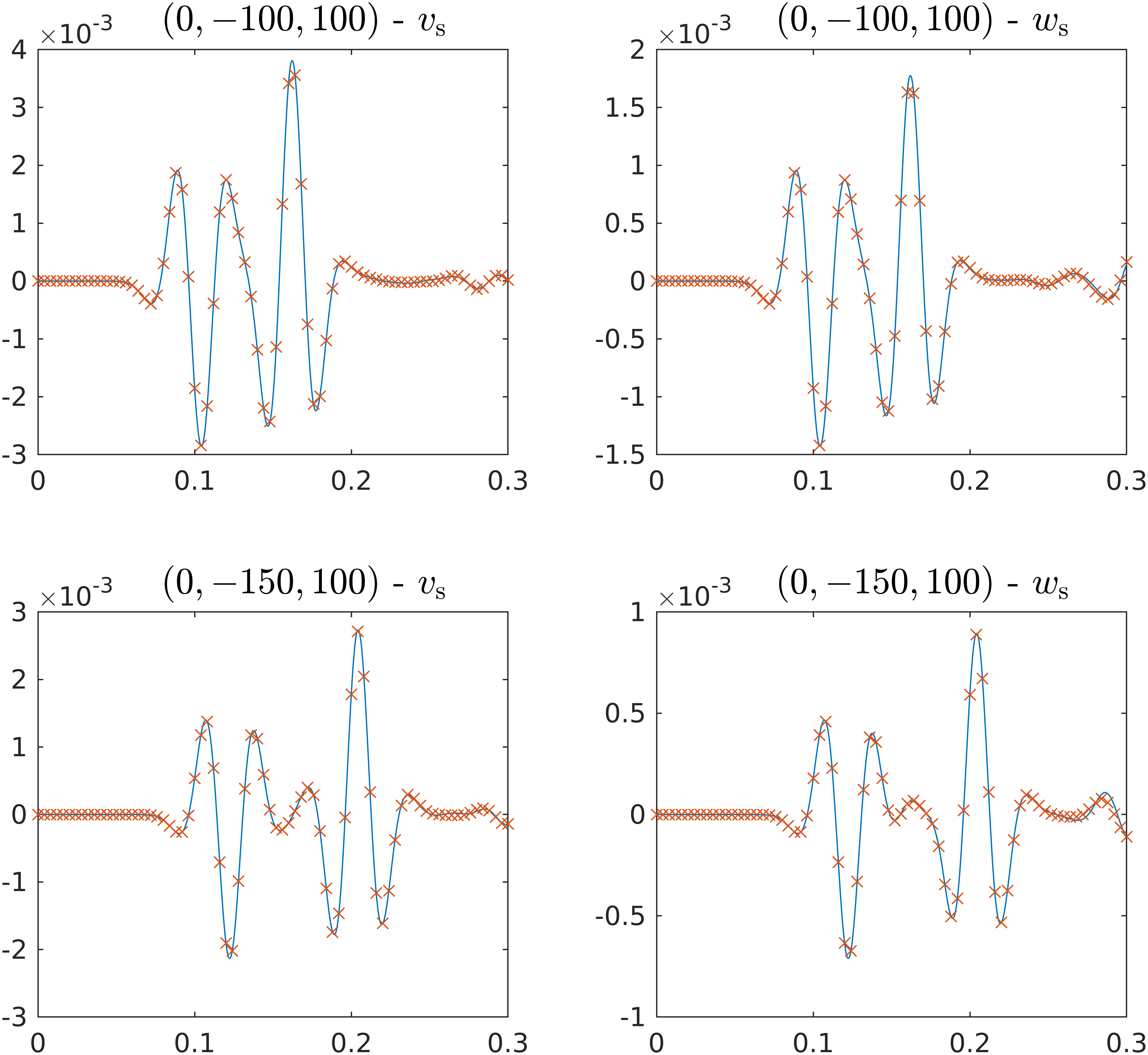
Figure 3: Simulation of the two-layered poroelastic model of Section 7.2.1, showing time histories of the velocity components $v_{\rm s}$ (left), $w_{\rm s}$ (right) at two receiver locations: DG (line) and semi-analytic (crosses). The upper row corresponds to receiver location $(x,y,z)=(0,-100,100)$  m and the lower row to $(x,y,z)=(0,-150,100)$ m.

7.2.2 Elastic-elastic

The following experiment has a similar set-up to the previous one: the computational domain is a cube $\Omega=[-2.5,2.5]\times[-2.5,2.5]\times[-2.5,2.5]$ m, with the plane $z=0$ forming the interface between elastic subdomains with the same moment tensor. The characteristic frequency of the Ricker wavelet has been increased to 2000 Hz and absorbing boundary conditions applied across the whole boundary. Material densities and wave speeds are given in Table 9.

Table 9: Densities and wave speeds for the elastic-elastic case in Section 7.2.2.

variable name	symbol	upper	lower
solid density	$\rho_{\mathrm{s}}$ (kg/m3)	2000	700
pressure wave speed	$c_{p}$ (m/s)	3500	2800
shear wave speed	$c_{s}$ (m/s)	2000	700

The computational domain $\Omega$ is partitioned by an irregular tetrahedral grid consisting of 35792 elements and 6858 vertices ($h_{\min}=0.12$ m and $h_{\max}=0.95$ m). For the grid, the element size is chosen to be 2 elements per shortest wavelength in both subdomains. We set the basis order to 4.

The solid velocity components $v_{\rm s}$ and $w_{\rm s}$ as functions of time are shown in Figure 4 for two receiver locations in the upper layer and two in the lower half layer (coordinates: (0 1 1), (0 0.68 0.5), (0 1 -1), (0 0.68 -0.5)). To achieve the fit we scaled the semi-analytic output by 0.5. The reason for this is that when applying cylinderical symmetry to the elastic wave equation the source term is scaled by 0.5 and this appears to be absent in the derivation in [11]. Apart from some minor boundary reflections for two components at the more distant locations from the source, the signal responses show excellent agreement with the semi-analytic solution “Gar6more3D”.

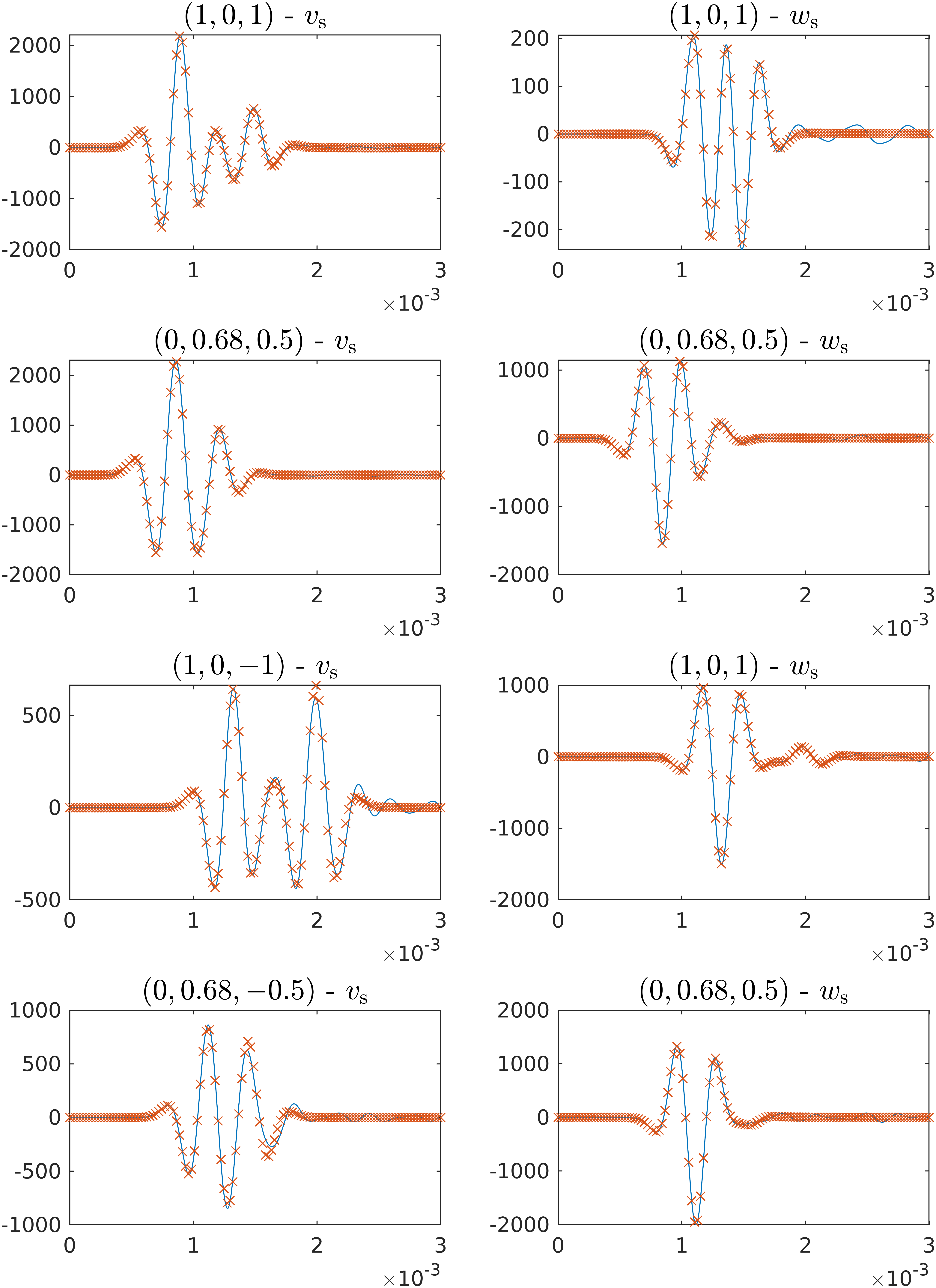
Figure 4: Simulation of the two-layered elastic model of Section 7.2.2, showing time histories of the velocity components $v_{\rm s}$ and $w_{\rm s}$ at four locations: DG (line) and semi-analytic (crosses).

7.3 Adjoint method

In this section we present a simple, but illuminating, example of the application of the adjoint method. The example was motivated by the example for the acoustic wave equation in section 3 of [14]. We consider an almost everywhere homogeneous cubical domain $\Omega=[0,5]\times[0,5]\times[0,5]$ m with one anomalous feature in a single element containing the point $[2.5,2.5,4]$ m where the solid and fluid densities are doubled. The homogeneous parameters are the same as the material parameters used in the convergence tests, Table 3. A point source is located at $[2.5,2.5,2]$ m and modelled as an explosive source with $M_{xx}=M_{yy}=M_{zz}=100$ N$\cdot$m. The central frequency of the Ricker wavelet is assumed to be 2000 Hz. Velocity data is then generated for the problem at 100 equally spaced receiver locations on the top surface $z=5$ m. Free surface boundary conditions were implemented on all 6 boundary surfaces.

On the other hand the reference model is assumed to be everywhere homogeneous with parameters given in Table 3. Letting $\bm{\theta}_{0}$ denote the parameter space for the anomalous model, and $\bm{\theta}$ denote the parameter space for the reference model, we may write the misfit functional as

$$\chi(\bm{\theta})=\frac{1}{2}\sum_{i\in\mathcal{I},r\in\mathcal{R}}\int_{0}^{T}[q_{i}(\bm{\theta},x_{r},t)-q_{i}(\bm{\theta}_{0},x_{r},t)]^{2}dt$$ (237)

The forward wavefield is propagated for $6/f_{0}=3\times 10^{-3}$ seconds and a snapshot shown in Figure 5. It is evident that considerable scattering has occurred. Examples of adjoint source wavelets $(\mathbf{q}-\mathbf{d})\delta(x-x_{r})\chi_{\mathcal{I}}$ are shown in Figure 6. Not surprisingly the central four wavelets contain the most information since they are closest to the anomaly, while the furthest two receivers contain further information due to the scattering on the sides of the wave field. Figure 7 shown snapshots of the forward wavefield and adjoint wavefield at times $.85\times 10^{-3},1.65\times 10^{-3},1\times 10^{-3}$ seconds. It is evident that the adjoint field focuses briefly on the anomalous feature, during which time the forward wavefront passes through the neighbourhood. Therefore the contribution to the Fréchet kernel $k_{\rho_{a}}$ is greatest during this non-trivial overlapping period. Figure 8 shows a snapshot of $k_{\rho_{a}}$. It is evident that the kernel’s centre contains the anomalous element, which extends into two tooth-like roots. The interference near the top surface is due to the early time overlap between the scattered forward wavefield and the initial evolution of the adjoint wavefield.

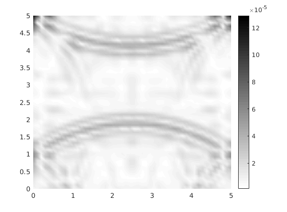
Figure 5: Snapshot of the forward wavefield at the final time $t=3\times 10^{-3}$ seconds through the plane $x=2.5$ m.

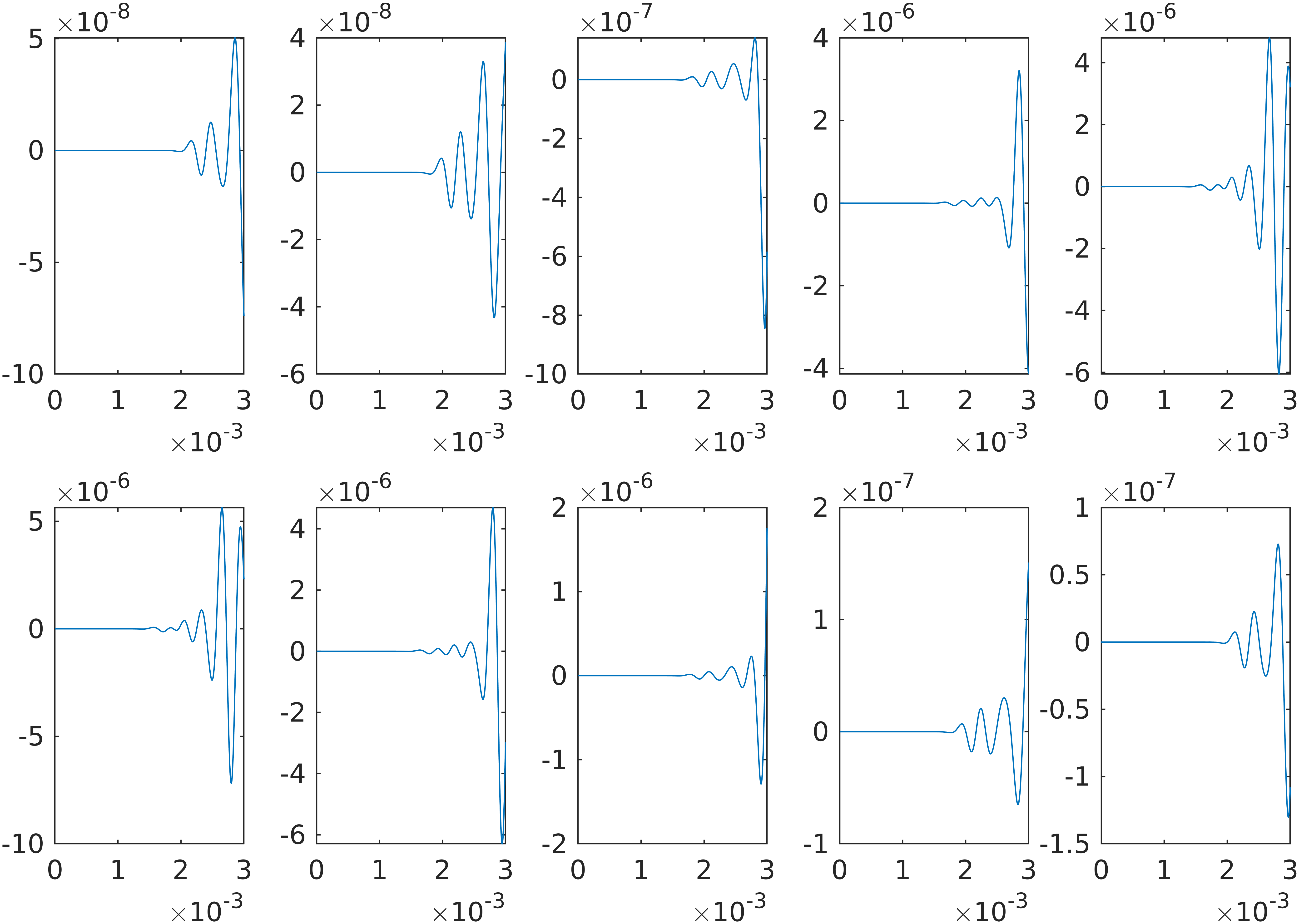
Figure 6: Examples of the $x$-component of adjoint source wavelets through the line $x=5.6$ m.

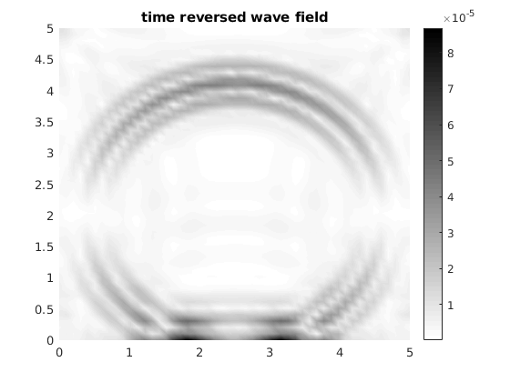
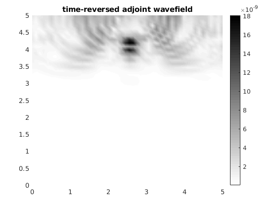
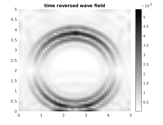
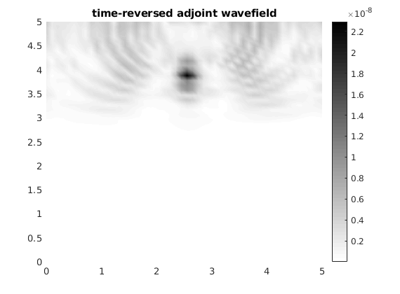
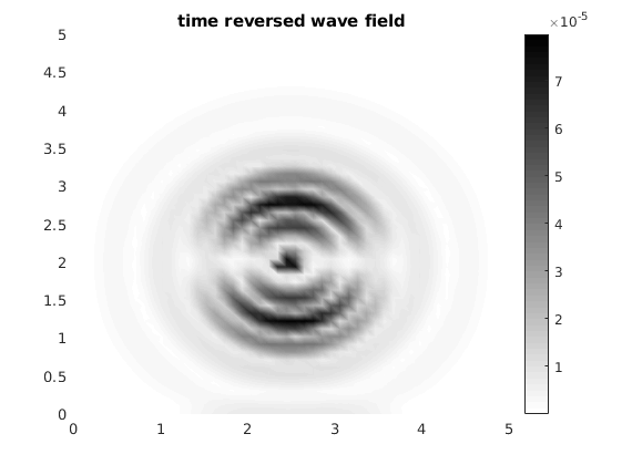
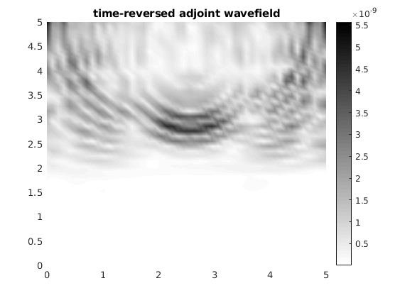
Figure 7: Snapshots of the foward (left) and adjoint (right) wavefields at times $1.85\times 10^{-3},1.65\times 10^{-3},1\times 10^{-3}$ seconds.

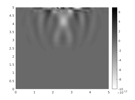
Figure 8: Snapshot of Fréchet kernel $k_{\rho_{a}}$ through the plane $x=2.5$ m.

8 Discussion

As with our previous two-dimensional work [12], our principal motivation for working in the DG framework was to obtain a forward solver for three-dimensional poroelastic wavefields that could accurately resolve material discontinuities. This is a necessary feature for groundwater tomographic applications, in which abrupt changes in porosity and permeability commonly occur between water-bearing and non-water-bearing strata. In our initial studies of related inverse problems we used the well-known SPECFEM code to simulate forward poroelastic wavefields. However, as discussed in section 6.2.1 of our previous paper, this approach does not naturally resolve discontinuities in porosity, whereas the DG approach, as we have shown in section 7.1, naturally deals with this. Furthermore, in applications to groundwater tomography, aquifer permeabilities can be quite large (up to $k\sim 10^{-7}\ \text{m}^{2}$, [2]), forcing one to operate simultaneously in high-frequency regimes (water-saturated subdomains) and low-frequency regimes (air-saturated subdomains). The elastic/poroelastic coupling is necessary since the usually much slower secondary P-wave puts a very significant computational burden on the forward solver because the mesh resolution is controlled by the shortest wavelength. One approach to model reduction in estimation problems, significantly reducing the computational burden, is to make an elastic approximation in some subdomains [19, 20] and, of course, the basement of an aquifer is plainly modelled as an elastic layer. Our implementation permits coupling between low frequency poroelastic, high frequency poroelastic and elastic subdomains.

With a certain loss of elegance, it is a simple extension to deal with non-isotropic domains and to add further attenuation mechanisms for modelling a viscoporoelastic system. However, since poroelastic inverse problems are extremely challenging, and we have been unable to find a satisfactory approach to solving even modest scale problems in two dimensions, our view is that there is still significant work to do before tackling inverse problems for non-isotropic domains.

The adjoint method is a necessary approach to reducing the computational burden of non-trivial inverse problems, especially those using gradient-based approaches to minimising a misfit functional or maximum a posteriori estimation (MAP) in the Bayesian framework. Again the equations have been derived with some generality permitting coupling between low and high frequency poroelastic and elastic domains. To our knowledge, the application of the adjoint method to poroelastic inverse problems has been little explored [24]. We prefer to work with bulk parameters like the Biot coefficient $\alpha$ and the coupling coefficient $M$ in estimation problems since it is less cumbersome, and then use sampling to estimate the real physical parameters of interest like porosity. In [24], on the other hand, Morency and Tromp have explored the adjoint method for two-dimensional poroelastic problems using the spectral element framework, and derived lengthy expressions for the Fréchet kernels for the underlying physical parameters. While they draw some parallels with the elastic case, there is much work to be done to fully explore the utility of the adjoint method for poroelastic inverse problems.

In our numerical simulations, for smaller examples, we used the well-established Matlab code of Hesthaven and Warburton [15]. As they acknowledge in their introduction, this becomes impractical for larger meshes; for these, we implemented the DG algorithm in C, using MPI for parallelism and METIS [16] to partition the mesh. Running on a standard desktop computer with four or six cores, this is typically faster than Matlab by a factor of about 4 or 5. The limiting factor seems likely to be the memory speed: in any language, the code must repeatedly traverse arrays much larger than the system’s memory caches (Cavaglieri and Bewley [10], whose low-storage IMEX schemes we used for stiff cases, mention this point in their abstract). More important than the speed is the scalability of the MPI code: for a large mesh, both the computational and the memory requirements can be distributed across many nodes of a cluster. At this point, communication costs become significant, or even dominant: the parallel processes need to synchronise by exchanging data at every Runge-Kutta stage (so, five times per time-step for the LSERK method that we used for non-stiff problems) and no computation takes place until all communication has finished. This tension between computational and communication costs leads to a not easily predicted optimal number of processes for any given problem. For example, on a mesh with about 150,000 elements and 84 nodes per element (polynomial degree 6), experimentation on the Viking cluster at the University of York suggested that execution time would be minimised by using somewhere around 50-60 cores; in the ever-changing environment of a shared cluster, more precise statements are impossible.

As permeability becomes smaller, the onset of stiffness in the low-frequency dissipative terms begins to demand unfeasibly small step lengths in any explicit Runge-Kutta method. In these cases, we used a hybrid implicit-explicit (IMEX) scheme in which the stiff terms are handled by the implicit part of the scheme and the rest of the system is handled by the explicit part. Our formulation is ideally suited to this type of scheme, because the equations in the implicit part can solved simply and explicitly, entirely eliminating the extra costs usually associated with implicit schemes. This gives convergence of the scheme but, unlike in all other regimes, we did not observe the convergence rates expected for the main hyperbolic system. Our interpretation of this is that the numerical errors associated with the dissipative terms dominate those associated with the hyperbolic system.

9 Conclusions

In this paper we developed a DG solver for a coupled three-dimensional poroelastic/elastic isotropic model incorporating Biot’s low- and high-frequency regimes in Hesthaven and Warburton’s framework [15]. Time integration was carried out using both low-storage explicit and (for the stiff case) implicit-explicit Runge-Kutta schemes. We considered free surface and absorbing boundary conditions, where the latter were modelled as outflows. Numerical experiments showed that, except for very stiff cases, the solver satisfied theoretical convergence rates. In stiff examples, IMEX time integration gave weaker convergence rates. We observed that the exact Riemann-problem-based numerical flux implementation resolves naturally all material discontinuities. We showed that the adjoint wavefield has a natural physical interpretation as a velocity/strain formulation of the Biot equation; this will be further explored in a forthcoming paper.

A MATLAB implementation of the DG schemes derived in this paper to accompany the Hesthaven-Warburton DG library is available from github:

https://github.com/nickdudleyward/dg_biot_3d_1.0

References

• [1] K. Aki and P.G. Richards. Quantitative Seismology. University Science Books, 1980.
• [2] J. Bear. Hydraulics of Groundwater. Dover, 1979.
• [3] M.A. Biot. Theory of propagation of elastic waves in a fluid saturated porous solid. I. Low frequency range. J. Acoust. Soc. Am., 28(2):168–178, 1956.
• [4] M.A. Biot. Theory of propagation of elastic waves in a fluid saturated porous solid. II. Higher frequency range. J. Acoust. Soc. Am., 28(2):179–191, 1956.
• [5] M.A. Biot. Mechanics of deformation and acoustic propagation in porous media. J. Appl. Phys., 33(4):1482–1498, 1962.
• [6] M.A. Biot and D.G. Willis. The elastic coefficients of the theory of consolidation. J. Appl. Mech., 24:594–601, 1957.
• [7] J.M. Carcione. Wave Fields in Real Media: Wave propagation in anisotropic, anelastic and porous media. Elsevier, 2015.
• [8] J.M. Carcione and G. Quiroga-Goode. Some aspects of the physics and numerical modeling of Biot compressional waves. J. Comput. Acoust., 3:261–280, 1995.
• [9] M.H. Carpenter and C.A. Kennedy. Fourth-order 2N-storage Runge-Kutta schemes. Technical report, NASA-TM-109112, 1994.
• [10] D. Cavaglieri and T. Bewley. Low-storage implicit/explicit Runge-Kutta schemes for the simulation of stiff high-dimensional ODE systems. J. Comput. Phys., 286:172–193, 2015.
• [11] J. Diaz and A. Ezziani. Analytical solution for wave propagation in stratified poroelastic medium. Part II: the 3D Case. eprint in arXiv, https://arxiv.org/abs/0807.4067, 2008. http://www.spice-rtn.org/library/software/Gar6more3D.
• [12] N.F. Dudley Ward, T. Lähivaara, and S. Eveson. A discontinuous Galerkin method for poroelastic wave propagation: The two-dimensional case. J. Comput. Phys., 350:690–727, 2017.
• [13] A. Fichtner. Full Seismic Waveform Modelling and Inversion. Springer, 2011.
• [14] A. Fichtner, H.-P. Bunge, and H. Igel. The adjoint method in seismology I. Theory. Phys. Earth Planet. In., 157:86–104, 2006.
• [15] J.S. Hesthaven and T. Warburton. Nodal Discontinuous Galerkin Methods: Algorithms, Analysis, and Applications. Springer, 2007.
• [16] George Karypis and Vipin Kumar. A fast and high quality multilevel scheme for partitioning irregular graphs. SIAM J. Sci. Comput., 20(1):359–392, 1998.
• [17] C.A. Kennedy and M.H. Carpenter. Additive Runge-Kutta schemes for convection-diffusion-reaction equations. Appl. Numer. Math., 44(1-2):139–181, 2003.
• [18] B. L. N. Kennett. The Seismic Wavefield. Volume I: Introduction and Theoretical Development. Cambridge University Press, 2001.
• [19] T. Lähivaara, N.F. Dudley Ward, T. Huttunen, J. Koponen, and J.P. Kaipio. Estimation of aquifer dimensions from passive seismic signals with approximate wave propagation models. Inverse Probl., 30(1):015003, 2014.
• [20] T. Lähivaara, N.F. Dudley Ward, T. Huttunen, Z. Rawlinson, and J.P. Kaipio. Estimation of aquifer dimensions from passive seismic signals in the presence of material and source uncertainties. Geophys. J. Int., 200:1662–1675, 2015.
• [21] T. Lähivaara, A. Malehmir, A. Pasanen, L. Kärkkäinen, J.M.J. Huttunen, and J.S. Hesthaven. Estimation of groundwater storage from seismic data using deep learning. Geophys. Prospect., 2019.
• [22] G.I. Lemoine, M. Yvonne Ou, and R.J. LeVeque. High-resolution finite volume modeling of wave propagation in orthotropic poroelastic media. SIAM J. Sci. Comput, 35(1):B176–B206, 2013.
• [23] R.J. LeVeque. Finite Volume Methods for Hyperbolic Problems. Cambridge University Press, 2002.
• [24] C. Morency, Y. Luo, and J. Tromp. Finite-frequency kernels for wave propagation in porous media based upon adjoint methods. Geophys. J. Int., 179(2):1148–1168, 2009.
• [25] K. Shukla, J. Chan, M. V. de Hoop, and P. Jaiswal. A weight-adjusted discontinuous Galerkin method for the poroelastic wave equation: Penalty fluxes and micro-heterogeneities. J. Comput. Phys., 403, 2020.
• [26] K. Shukla, J. S. Hesthaven, J. M. Carcione, R. Ye, J. de la Puente, and P. Jaiswal. A nodal discontinuous Galerkin finite element method for the poroelastic wave equation. Computat. Geosci., 2018.
• [27] J. Tromp, D. Komatitsch, and Q. Liu. Spectral-element and adjoint methods in seismology. Commun. Comput. Phys., 3(1):1–32, 2008.
• [28] L.C. Wilcox, G. Stadler, T. Bui-Thanh, and O. Ghattas. Discretely exact derivatives for hyperbolic PDE-constrained optimization problems dicretized by the discontinuous Galerkin method. J. Sci. Comput., 63:138–162, 2015.
• [29] L.C. Wilcox, G. Stadler, C. Burstedde, and O. Ghattas. A high-order discontinuous Galerkin method for wave propagation through coupled elastic-acoustic media. J. Comput. Phys., 229:9373–9396, 2010.
• [30] Q. Zhan, M. Zhuang, and Q. H. Liu. A compact upwind flux with more physical insight for wave propagation in 3-d poroelastic media. IEEE Transactions on Geoscience and Remote Sensing, 56(10):5794–5801, 2018.
• [31] Q. Zhan, M. Zhuang, Y. Mao, and Q. H. Liu. Unified Riemann solution for multi-physics coupling: Anisotropic poroelastic/elastic/fluid interfaces. J. Comput. Phys., 402, 2020.