Improved mixing time for $k$-subgraph sampling

Abstract

Understanding the local structure of a graph provides valuable insights about the underlying phenomena from which the graph has originated. Sampling and examining $k$-subgraphs is a widely used approach to understand the local structure of a graph. In this paper, we study the problem of sampling uniformly $k$-subgraphs from a given graph. We analyse a few different Markov chain Monte Carlo (MCMC) approaches, and obtain analytical results on their mixing times, which improve significantly the state of the art. In particular, we improve the bound on the mixing times of the standard MCMC approach, and the state-of-the-art MCMC sampling method PSRW, using the canonical-paths argument. In addition, we propose a novel sampling method, which we call recursive subgraph sampling RSS, and its optimized variant RSS+. The proposed methods, RSS and RSS+, are provably faster than the existing approaches. We conduct experiments and verify the uniformity of samples and the time efficiency of RSS and RSS+.

1 Introduction

Graphs are used to model complex real-world data in a wide range of domains, such as, sociology, biology, ecology, transportation, telecommunications, and more. Understanding the structural properties of graphs, at different levels of granularity, provides valuable insights about the underlying phenomena and processes that generate the corresponding graph data. A compelling approach to explore the structural properties of a graph, or a collection of graphs, at a fine scale, is to extract information about small-size subgraphs related to their connectivity patterns, interactions, and other features of interest [9, 21, 17, 24, 29]. For instance, the high ratio of closed triangles observed in social networks has been considered a manifestation of social affinity observed in human society and which leads to forming tightly-knit groups. As a concrete example, it has been found that the ratio of closed triangles is higher in facebook, which is primarily an online social network, than in twitter, which is used as a platform for news dissemination [18].

More interesting structural properties and hidden patterns in the graph data can be revealed by examining larger subgraphs, e.g., subgraphs of size $k$, or $k$-subgraphs. Unfortunately, the number of $k$-subgraphs in a given graph increases exponentially with $k$, and enumerating all possible $k$-subgraphs becomes prohibitive. To address this challenge one usually resorts to sampling. To make the sampling idea viable requires obtaining a representative subset of the set of all $k$-subgraphs, or equivalently, sampling $k$-subgraphs uniformly at random, which is a challenge by itself. As a result, the problem of uniform sampling $k$-subgraphs, has been extensively studied in data mining, statistics, and theoretical computer science [1, 4, 6, 7, 10, 14, 22, 25, 27].

In this paper, we study the problem of sampling uniformly at random $k$-subgraphs from a given input graph. Among the different methodologies that have been proposed, we focus on the Markov chain Monte Carlo (MCMC) approach [20], and in particular on the Metropolis-Hastings algorithm (MH) [11]. The high-level idea is to sample from the stationary distribution of a Markov chain, whose set of states is the set of $k$-subgraphs, by performing a random walk. The MH algorithm [11] is used to ensure that the stationary distribution, and thus, the sampling, is uniform. An important theoretical question is to upper bound the mixing time of the random walk, which is the time needed for the empirical sampling distribution to be close enough to the stationary distribution.

We present improved results for the mixing time of Markov chains designed for uniform sampling of $k$-subgraphs. Our starting point is the recent work of Bressan et al. [7], who analyze a MCMC method and show that it mixes in time $\tilde{\mathcal{O}}((k!)^{2}\Delta^{2k}|V|^{2})$, where $|V|$ is the number of nodes in the input graph, $\Delta$ is a maximum node degree, and $\tilde{\mathcal{O}}(\cdot)$ is used to suppress logarithmic and other lower-term factors.

Our first result is to analyze the Markov chain with the MH algorithm using the technique of canonical paths [23] and obtain an upper bound on the mixing time of $\tilde{\mathcal{O}}(k!\Delta^{k}(D+k)|V|)$, where $D$ is a diameter of the graph. Our bound is a significant improvement of the bound of Bressan et al. [7].

Next, we proceed to improve this bound even further, by introducing a novel Markov chain to perform the random walk. In particular, we propose a technique based on recursive subgraph sampling (RSS), and a further improvement called RSS+, which exploits the fact that we can easily sample $2$-subgraph uniformly at random in time $\mathcal{O}(1)$: sampling a $2$-subgraph is just sampling an edge on the input graph. In turn, this gives us a way to sample a $3$-subgraph uniformly at random by applying the MH approach. The idea can be applied recursively for all $k$. The complexity of the RSS scheme is $\tilde{\mathcal{O}}(c^{k-3}(k!)^{2}((k-1)!)^{2}\Delta^{k-3})$, where $c$ is a constant. Although this bound is still large, assymptotically is a big improvement compared to the previous work, and to our MCMC bound. Furthermore, in practice, $k$ is typically taken to be a small constant, i.e., $|V|\gg k$.

We experimentally evaluate our methods for $k=3,4,5$ and we verify the superiority of the RSS scheme against the MCMC method, and the state-of-the-art PSRW algorithm [26]. We also evaluate RSS and RSS+ for values of $k$ up to 10; we present this in the Appendix. As it has been observed by other researchers, we confirm that the theoretical bounds are overly pessimistic, and in practice it suffices to run the random walk for a significantly smaller number of steps.

Our key contributions are as follows:

• We apply the technique of canonical paths [23] to obtain a bound on the mixing time of the standard MCMC method, which is a significant improvement over the state of the art.

• We propose novel $k$-subgraph sampling algorithms, RSS and RSS+, whose computational costs further improve the mixing time of MCMC sampling.

• We obtain a bound on the mixing time of the PSRW method [26], which was left open by the authors.

• We conduct an experimental evaluation and show that RSS and RSS+ are significantly faster compared to MCMC sampling and PSRW.

The rest of this paper is organized as follows. We start by reviewing the related work in Section 2. Our algorithms, analysis, and main results are presented in Section 3. In Section 4 we discuss our experimental evaluation, and finally, Section 5 is a short conclusion.

The proofs of our lemmas and claims can be found in Appendix A, while additional experimental results are presented in Appendix B.

2 Related work

Sampling $k$-subgraphs uniformly at random is computationally expensive. The number of possible $k$-subgraphs of $G=(V,E)$ is $\binom{|V|}{k}=\mathcal{O}(|V|^{k})$. Enumerating all of them is intractable. Hence, the approximation of sampling has been studied [19, 26, 7, 5].

A standard approach is to apply Markov chain Monte Carlo (MCMC) sampling with the Metropolis-Hastings (MH) technique [19, 26, 7, 5]. This approach performs a random walk on a graph whose nodes are all $k$-subgraphs of an input graph $G=(V,E)$, and two $k$-subgraphs are adjacent if they differ by one node. The graph of $k$-subgraphs is defined as the $k$-state graph in the next section. By performing random walk on the $k$-state graph we can obtain a uniform sample of $k$-subgraphs. Bressan et al. [7] study the conductance of the $k$-state graph and show that it increases exponentially, which directly implies that the mixing time of a simple random walks on it also increases exponentially; the upper bound of the mixing time is $\tilde{\mathcal{O}}((k!)^{2}|V|^{2}\Delta^{2k})$, where $|V|$ is the number of nodes and $\Delta$ is the maximum degree of the given graph $G$. They also show that even when the given graph has low conductance, the mixing time can be exponential.

Wang et al. [26] notice that a $k$-subgraph sample can be obtained by sampling an edge from the graph of $(k-1)$-subgraphs, i.e., the $(k-1)$-state graph. This method is named pairwise subgraph random walk (PSRW). They prove that PSRW samples a $k$-subgraph uniformly at random. Since a random walk on the $(k-1)$-state graph has faster mixing time than on the $k$-state graph, PSRW is more efficient than the standard MCMC approach. It is, however, still exponential.

As another approach, Bressan et al. [7] propose a sampling algorithm that uses the color-coding technique [3]. The computational cost of their method is $\mathcal{O}(c^{k}|E|)$. In this paper, we focus on Markov chain approaches, and we analyse the mixing time of $k$-state graphs. Thus, we exclude this approach from our comparisons for the sake of consistency.

3 Subgraph sampling

3.1 Terminology and problem definition

We start with an undirected graph $G=(V,E)$. Let $H=(V_{H},E_{H})$ be a connected $k$-subgraph of $G$, that is, $H$ is a connected vertex-induced subgraph of $G$ containing exactly $k$ nodes. More precisely, $V_{H}\subseteq V$, $|V_{H}|=k$, $E_{H}=\{(u,v)\in E\mid u,v\in V_{H}\}$, and $H$ is connected. We use the notation $H\subseteq_{k}G$ to denote that $H$ is a connected $k$-subgraph of $G$.

Let $V^{(k)}$ be a set of all connected $k$-subgraphs of $G$, i.e., $V^{(k)}=\{H\subseteq_{k}G\}$. We construct a graph $G^{(k)}$ whose node set is $V^{(k)}$. In the graph $G^{(k)}$, two nodes $H=(V_{H},E_{H})$ and $F=(V_{F},E_{F})$ are adjacent if and only if the sets $V_{H}$ and $V_{F}$ differ by exactly one node. Hence, the edge set $E^{(k)}$ of the constructed graph $G^{(k)}$ is:

$$\small E^{(k)}=\{(H,F)\mid H,F\in V^{(k)}\text{ and }|V_{H}\cap V_{F}|=k-1\}.$$

The graph $G^{(k)}=(V^{(k)},E^{(k)})$ defined above is called the $k$-state graph of $G$. Note that $G=(V,E)$ can also be seen as $G^{(1)}=(V^{(1)},E^{(1)})$ for the case of $k=1$.

We denote by $\Delta$ the maximum degree of a node in $G$, and by $\Delta_{k}$ the maximum degree of a node in $G^{(k)}$. We denote by $d(u)$ the degree of node $u$ in the graph that $u$ belongs; e.g., if $H\subseteq_{k}G$, then $d(H)$ denotes the degree of $H$ in the $k$-state graph $G^{(k)}$. Note that Bressan et al. [7] study $k$-state graphs and upper bound the maximum degree of $k$-subgraph by $\Delta_{k}\leq k\Delta$. They also give an upper bound of the number $|V^{(k)}|$ of $k$-subgraphs by $|V^{(k)}|\leq(k-1)!\Delta^{k-1}|V|$.

The problem we consider in this paper is to sample uniformly at random a node from the graph $G^{(k)}$, given a graph $G$ and an integer $k$. More formally:

Problem 3.1 (Uniform $k$-subgraph sampling).

Given a graph $G=(V,E)$ and a number $k\in\mathbb{N}$, with $1<k<|V|$, sample a connected $k$-subgraph $H\subseteq_{k}G$ uniformly at random.

3.2 Overview

Before presenting the proposed solution for Problem 3.1, we review the standard Markov Chain Monte Carlo (MCMC) approach, and introduce concepts needed in our analysis.

MCMC method. The MCMC method is used to obtain a sample from a desired distribution by designing a Markov chain whose stationary distribution corresponds to the desired distribution. Let $\Omega=\{0,\ldots,m-1\}$ be a state space, and $p(u,v)$ be the transition probability between states $u,v\in\Omega$, also represented as a matrix of transition probabilities $\mathbf{P}\in[0,1]^{m\times m}$, with $\mathbf{P}_{u,v}=p(u,v)$. Starting from $x\in\Omega$, the probability that a random walk visits $y\in\Omega$ in exactly $t$ steps is given by $(\mathrm{e_{x}}\mathbf{P}^{t})_{y}$, where $\mathrm{e_{x}}$ is a unit row vector having 1 in $x$-th coordinate. An ergodic Markov chain has a stationary distribution $\pi\in[0,1]^{m}$, given by $\pi=\pi\mathbf{P}$. Hence, by conducting a sufficiently long random walk on the chain we can obtain a sample from the distribution $\pi$.

Metropolis-Hastings algorithm. The Metropolis-Hastings algorithm (MH) [11] is a standard technique to convert a stationary distribution $\pi$ of a Markov chain to a desired stationary distribution $\pi^{\prime}$. It adds one step in MCMC sampling: a transition from $x\in\Omega$ to $y\in\Omega$ is accepted with probability $\min\left\{1,\frac{\pi^{\prime}_{y}/\pi_{y}}{\pi^{\prime}_{x}/\pi_{x}}\right\}$, otherwise, the walk stays at $x$. The resulting random walk has stationary distribution $\pi^{\prime}$.

Mixing time of MCMC. Mixing time provides a measure of efficiency of the sampling method by quantifying how fast the sampling distribution $\mathrm{e_{x}}\mathbf{P}^{t}$, starting at state $x$, approaches the stationary distribution $\pi$ [23, 13]. The mixing time $\tau(\varepsilon)$ is defined as the minimum number of random-walk steps required to achieve quality of approximation $\varepsilon$. In particular,

$$\tau_{x}(\varepsilon)=\arg \min_{t\in\mathbb{N}}\left\{\frac{1}{2}\sum_{y\in\Omega}|(\mathrm{e_{x}}\mathbf{P}^{\ell})_{y}-\pi_{y}|\leq\varepsilon,\text{ for all }\ell\geq t\right\},$$

$$\text{and }~{}\tau(\varepsilon)= \max_{x\in\Omega}\tau_{x}(\varepsilon).$$

Canonical paths [23]. This term refers to a proof technique used to upper bound the mixing time of a Markov chain. Given a Markov chain with state space $\Omega$, we define an underlying directed graph $(\Omega,E_{M})$, where $E_{M}$ is a set of directed edges between states in $\Omega$ with positive transition probability, i.e., $E_{M}=\{(u,v)\in\Omega\times\Omega\mid p(u,v)>0\}$. A canonical path $\gamma_{xy}$ is a path from $x\in\Omega$ to $y\in\Omega$ on the graph $(\Omega,E_{M})$. A set of canonical paths $\Gamma$ consists of canonical paths for each ordered pair of distinct states $x,y\in\Omega$. An upper bound on the mixing time can be calculated as follows [13, Proposition 12.1]:

(1) $$\tau_{x}(\varepsilon)\leq\overline{\rho}\,(\ln{\pi_{x}}^{-1}+\ln\varepsilon^{-1}),$$

where $$\overline{\rho}=\max_{(u,v)\in E_{M}}\frac{1}{Q(u,v)}\sum_{\gamma_{xy}\in\Gamma\wedge\gamma_{xy}\ni(u,v)}\pi_{x}\pi_{y}|\gamma_{xy}|,$$

$Q(u,v)=\pi_{u}p(u,v)=\pi_{v}p(v,u)$, and $|\gamma_{xy}|$ is the length of the path $\gamma_{xy}$. The tightness of the upper bound depends on the choice of canonical paths. Intuitively, we want to select canonical paths so that no single edge is used by too many paths. More details can be found in the excellent book of Jerrum and Sinclair [13].

3.3 Markov Chain Monte Carlo (MCMC) approach

A simple solution to $k$-subgraph sampling (Problem 3.1) is to apply the MCMC and MH methods discussed above. The method is shown in Algorithm 1, and we refer to it as MCMCSampling. The main observation is that the stationary distribution of a random walk in an undirected graph is proportional to the node degrees, thus, adding the acceptance probability step in line 9, according to MH, leads to uniform sampling. Note that the condition in line 6 adds a $\frac{1}{2}$-probability self-loop to ensure non-periodicity.

Algorithm 1 MCMCSampling

1:Graph $G=(V,E)$, subgraph size $k$, error $\varepsilon>0$

2:$H\subseteq_{k}G$ sampled from $V^{(k)}$ uniformly at random

3:$v_{c}\leftarrow$ arbitrary node in $G^{(k)}$

4:$N_{c}\leftarrow$ neighbor nodes of $v_{c}$ in $G^{(k)}$

5:for $\lceil t_{k}^{\mathrm{MCMC}}(\varepsilon)\rceil$ times do

6:    if $\mathit{random}(0,1)<\frac{1}{2}$ then

7:         $v_{n}\leftarrow$ randomly selected node from $N_{c}$

8:         $N_{n}\leftarrow$ neighbor nodes of $v_{n}$ in $G^{(k)}$

9:         if $\mathit{random}(0,1)<\min\left\{1,\frac{d(v_{c})}{d(v_{n})}\right\}$ then

10:             $v_{c}\leftarrow v_{n},N_{c}\leftarrow N_{n}$

11:         end if

12:    end if

13:end for

14:return $v_{c}$

To bound the mixing time of MCMCSampling, we apply the canonical-paths technique. First note that the Markov chain of MCMCSampling is on $G^{(k)}=(V^{(k)},E^{(k)})$. We choose a canonical path $\gamma_{xy}$ to be one of the shortest paths from $x$ to $y$ on $G^{(k)}$. The length of the path $|\gamma_{xy}|$ is bounded by the diameter of $G^{(k)}$, which in turn can be bounded using the following Lemma.

Lemma 3.1 (Diameter of $k$-state graph $G^{(k)}$).

The diameter of $k$-state graph $G^{(k)}$ is at most $(D+k-1)$, where $D$ is a diameter of $G$.

On the other hand, it is possible to construct problem instances in which the graph $G^{(k)}$ has a bottleneck edge, i.e., $V^{(k)}$ consists of two parts which are connected by just one edge. Then,

$$\overline{\rho} = \max_{(u,v)\in E_{M}}\frac{1}{Q(u,v)}\sum_{\gamma_{xy}\in\Gamma\wedge\gamma_{xy}\ni(u,v)}\pi_{x}\pi_{y}|\gamma_{xy}|$$

$$\leq \max_{(u,v)\in E_{M}}2\Delta_{k}|V^{(k)}|\sum_{\gamma_{xy}\in\Gamma\wedge\gamma_{xy}\ni(u,v)}\frac{1}{|V^{(k)}|^{2}}(D+k-1)$$

$$\leq 2k\Delta\frac{1}{|V^{(k)}|}(D+k-1)\max_{(u,v)\in E_{M}}|\{\gamma\in\Gamma\mid\gamma\ni(u,v)\}|$$

$$\leq 2k\Delta\frac{1}{|V^{(k)}|}(D+k-1)\left(\frac{|V^{(k)}|}{2}\right)^{2}$$

$$\leq \frac{1}{2}k!\Delta^{k}(D+k-1)|V|,$$

where $\pi_{x}=\frac{1}{|V^{(k)}|}$ for all $x\in V^{(k)}$, $p(u,v)\geq\frac{1}{2\Delta_{k}}$ for all $(u,v)$, $\Delta_{k}$ is the maximum degree in $G^{(k)}$, and $\Delta_{k}\leq k\Delta$ [7]. The largest value for $\max_{(u,v)\in E_{M}}|\{\gamma\in\Gamma\mid\gamma\ni(u,v)\}|$ on a graph with $|V^{(k)}|$ nodes is achieved when $G^{(k)}$ consists of two parts, each of which contains $\frac{|V^{(k)}|}{2}$ nodes, and they are connected by a single edge $(u,v)$. Since any path from a state in the one part to a state in the other part goes through $(u,v)$, we can bound $|\{\gamma\in\Gamma\mid\gamma\ni(u,v)\}|$ by $\left(\frac{|V^{(k)}|}{2}\right)^{2}$. Following Bressan et al., we use the bound $|V^{(k)}|\leq(k-1)!\Delta^{k-1}|V|$. An upper bound on the mixing time can now be obtained using Inequality (1):

$$t_{k}^{\mathrm{MCMC}}(\varepsilon) \leq \max_{x\in V^{(k)}}\overline{\rho}(\ln{\pi_{x}}^{-1}+\ln\varepsilon^{-1})$$

$$\leq \frac{1}{2}k!\Delta^{k}(D+k-1)|V|(k\ln|V|+\ln\varepsilon^{-1})$$

$$= \mathcal{O}(k!k\Delta^{k}(D+k)|V|\ln|V|).$$

The mixing time gives a bound on the number of random-walk steps required to obtain one sample. For the total computational cost of MCMCSampling, we also need to consider the cost per random-walk step. The number of neighbor nodes from a node in $G^{(k)}$ is $\mathcal{O}(k^{2}\Delta)$, and it takes $\mathcal{O}(k^{2})$ to check whether such a neighbor is connected, giving a cost of $\mathcal{O}(k^{4}\Delta)$ per random-walk step. The total cost of MCMCSampling is $\mathcal{O}(k!k^{5}\Delta^{k+1}(D+k)|V|\ln|V|)$.

Based on the analysis so far, we obtain the following results regarding the mixing time and the computational cost of MCMCSampling.

Lemma 3.2 (Mixing time).

The mixing time of the MCMCSampling algorithm is upper-bounded by $\frac{1}{2}k!\Delta^{k}(D+k-1)|V|(k\ln|V|+\ln\varepsilon^{-1})$ $=\mathcal{O}(k!k\Delta^{k}(D+k)|V|\ln|V|)$.

Theorem 3.3 (Computational cost).

The running time of the MCMCSampling algorithm is $\mathcal{O}(k!k^{5}\Delta^{k+1}(D+k)|V|\ln|V|)$.

3.4 Recursive subgraph sampling

MCMCSampling has provable guarantee on the mixing time, however, its complexity is prohibitive. Thus, we would like to develop an improved sampler with lower complexity. Next, we develop a recursive subgraph sampling (RSS) algorithm, which also samples a connected $k$-subgraph from a given graph with uniform probability. RSS is shown in Algorithms 2 and 3. The main function $\textsc{Uniform\-Sampling}(G,k,\varepsilon)$ and the subroutine $\textsc{Degree\-Prop\-Sampling}(G,k,\varepsilon)$ call each other $(k-3)$ times in a recursive manner.

Algorithm 2 Recursive subgraph sampling (RSS)

1:Graph $G=(V,E)$, subgraph size $k$, error $\varepsilon>0$

2:$H\subseteq_{k}G$ sampled from $V^{(k)}$ uniformly at random

3:function UniformSampling($G,k,\varepsilon$)

4:    if $k=2$ then

5:         return a uniformly-sampled edge from $E$

6:    end if

7:    while TRUE do

8:         $v\leftarrow$DegreePropSampling($G,k-1,\varepsilon$)

9:         $u\leftarrow$ uniformly-sampled neighbor of $v$ in $G^{(k-1)}$

10:         $H\leftarrow$ $k$-subgraph with nodes in $v$ and $u$

11:         $m\leftarrow$ number of $(k-1)$-subgraphs in $H$

12:         if $\mathit{random}(0,1)<\frac{1}{\binom{m}{2}}$  then

13:             return $H$

14:         end if

15:    end while

16:end function

Algorithm 3 Sampling $k$-subgraph prop. to its degree in $G^{(k)}$

1:Graph $G=(V,E)$, subgraph size $k$, error $\varepsilon>0$

2:$v\subseteq_{k}G$ sampled from $V^{(k)}$ with probability proportional to its degree

3:function DegreePropSampling($G,k,\varepsilon$)

4:    if k = 2 then

5:         return an edge $(u,v)\in E$ with probability proportional to $(d(u)+d(v)-2)$

6:    end if

7:    $v_{c}\leftarrow$ UniformSampling($G,k,\varepsilon$)

8:    $d_{c}\leftarrow$ degree of $v_{c}$

9:    for $\lceil t_{k}(\varepsilon)\rceil$ times do

10:         if $\mathit{random}(0,1)<\frac{1}{2}$ then

11:             $v_{n}\leftarrow$ UniformSampling($G,k,\varepsilon$)

12:             $d_{n}\leftarrow$ degree of $v_{n}$

13:             if $\mathit{random}(0,1)<\frac{d_{n}}{d_{c}}$ then

14:                 $v_{c}\leftarrow v_{n}$, $d_{c}\leftarrow d_{n}$

15:             end if

16:         end if

17:    end for

18:    return $v_{c}$

19:end function

The key observation is that sampling a 2-subgraph (edge) can be done in 2 steps: (1) sampling a node in $G$ with probability proportional to its degree; and (2) sampling uniformly an adjacent edge. This approach can be generalized to any $k>2$ as follows:

• sample a node $v$ in $G^{(k-1)}$ with probability proportional to its degree;

• sample uniformly at random an edge adjacent to $v$; denote this edge by $(v,u)\in E^{(k-1)}$.

• output a $k$-subgraph $H$ whose node set is the union of nodes of $v$ and $u$ with appropriate probability.

In the proposed RSS approach, step (1) is performed in $\textsc{Degree\-Prop\-Sampl\-ing}(G,k-1,\varepsilon)$, while steps (2) and (3) are performed in $\textsc{Uniform\-Sampl\-ing}(G,k,\varepsilon)$. We now discuss these two functions in more detail.

DegreePropSampling. To sample a node $v$ in $V^{(k)}$ with probability proportional to its degree in the state graph $G^{(k)}$, we apply the MH algorithm on a complete graph. Let us assume we can sample $v_{c}$ in $V^{(k)}$ uniformly at random, which is done by $\text{\sc Uniform}\-\textsc{Sampl\-ing}(G,k,\varepsilon)$ as explained later. Starting from $v_{c}$ we then sample a next state $v_{n}\in V^{(k)}$ uniformly at random. This is regarded as a random walk on the complete graph with nodes $V^{(k)}$. Since those samples are uniform, the stationary distribution is uniform, $\pi_{x}\sim 1$, and needs to be converted into $\pi_{x}\sim d(x)$ for any $x\in V^{(k)}$. Hence, we calculate the degrees $d(v_{c})$ and $d(v_{n})$, and accept $v_{n}$ as a new node $v_{c}$ with probability $\min\left\{1,\frac{d(v_{n})}{d(v_{c})}\right\}$. If we continue this walk for more than $t_{k}(\varepsilon)$ steps, $v_{c}$ becomes an approximate sample of $V^{(k)}$ with probability proportional to its degree.

We calculate an upper bound on the mixing time $t_{k}(\varepsilon)$ of $\textsc{Degree\-Prop\-Sampling}(G,k,\varepsilon)$ by applying again the canonical-paths argument. A crucial element of the construction is that the underlying graph of the Markov chain is the complete graph with $|V^{(k)}|$ nodes. The target stationary distribution is $\pi_{v}=\frac{d(v)}{Z}$, where $Z=\sum_{v\in V^{(k)}}d(v)=2|E^{(k)}|\leq k\Delta|V^{(k)}|$, and $Z\geq|V^{(k)}|$. The transition probability from a node $u$ to $v$ is $p(u,v)=\frac{1}{2|V^{(k)}|}\min\left\{1,\frac{d(v)}{d(u)}\right\}$, and $Q(u,v)=\pi_{u}p(u,v)=\frac{d(u)}{Z}\frac{1}{2|V^{(k)}|}\min\left\{1,\frac{d(v)}{d(u)}\right\}=\frac{\min\{d(v),d(u)\}}{2Z|V^{(k)}|}$. The quantity $\overline{\rho}$ is calculated as follows:

$$\overline{\rho} = \max_{(u,v)\in V^{(k)}\times V^{(k)}}\frac{1}{Q(u,v)}\sum_{\gamma_{xy}\in\Gamma\wedge\gamma\ni(u,v)}\pi_{x}\pi_{y}|\gamma_{xy}|$$

$$= \max_{(u,v)\in V^{(k)}\times V^{(k)}}\frac{2Z|V^{(k)}|}{\min\{d(v),d(u)\}}\frac{d(u)}{Z}\frac{d(v)}{Z}$$

$$= 2\frac{|V^{(k)}|}{2|E^{(k)}|}\max_{u\in V^{(k)}}d(u)$$

$$\leq 2k\Delta.$$

A bound on mixing time $t_{k}(\varepsilon)$ is obtained by

$$t_{k}(\varepsilon) \leq \max_{x\in V^{(k)}}\overline{\rho}\left(\ln\left(\frac{Z}{d(x)}\right)+\ln\varepsilon^{-1}\right)$$

$$\leq \overline{\rho}(\ln(k\Delta|V^{(k)}|)+\ln\varepsilon^{-1})$$

$$\leq 2k\Delta(\ln k+\ln\Delta+k\ln|V|+\ln\varepsilon^{-1})$$

$$= \mathcal{O}(k^{2}\Delta\ln|V|).$$

The total cost of $\textsc{Degree\-Prop\-Sampling}(G,k,\varepsilon)$ is $D_{k}=\mathcal{O}(k^{2}\Delta\ln|V|U_{k})$, where $U_{k}$ is the total computational cost of $\textsc{Uniform\-Sampling}(G,k,\varepsilon)$.

Note that $\textsc{Degree\-Prop\-Sampling}(G,2,\varepsilon)$ runs in constant time $\mathcal{O}(1)$, by pre-computing $(d(u)+d(v)-2)$ for each edge $(u,v)\in E$, which is the degree of 2-subgraph with nodes $\{u,v\}$, on $G^{(2)}$.

UniformSampling. We now discuss how to sample a $k$-subgraph uniformly at random. We first call $\text{\sc Degree\-Prop}\-\textsc{Sampling}(G,k-1,\varepsilon)$ and obtain $v$ in $V^{(k-1)}$ with probability proportional to its degree. Then we sample a neighbor state $u$ of $v$, uniformly at random, and then we obtain the subgraph $H$ whose nodes are the union of nodes in $v$ and $u$. When $k=2$, the subgraph $H$ is an uniform sample among all 2-subgraphs (edges). When $k>2$, however, the number of edges in $E^{(k-1)}$ that outputs this same $H$ is equal to the number of edges among $\{F\subseteq_{k-1}H\}$; let $m$ be the number of such $F$. The subgraph $H$ is accepted with probability $1/\binom{m}{2}$. If accepted, $H$ is the output subgraph. If rejected, we repeat until some subgraph is accepted. Note that $m$ is at most $k$. Hence, on expectation we have to repeat the process $\binom{m}{2}\leq\binom{k}{2}=\mathcal{O}(k^{2})$ times.

Thus, the computational complexity of $\text{\sc Uniform}\-\textsc{Sampling}(G,k,\varepsilon)$ subroutine is $U_{k}=\mathcal{O}(k^{2}D_{k-1})$, where $D_{k-1}$ is the computational cost of $\text{\sc Degree\-Prop}\-\textsc{Sampling}(G,k-1,\varepsilon)$. Unrolling the recurrences we obtain the overall complexity of RSS,

$$U_{k} = \mathcal{O}(c^{k-3}(k!)^{2}((k-1)!)^{2}\Delta^{k-3}(\ln|V|)^{k-3})\,,$$

where $c$ is a constant independent of $k$, $\Delta$, $|V|$ and the other variables. We obtain the following theorem.

Theorem 3.4 (Computational cost of RSS).

RSS takes time $\mathcal{O}(c^{k-3}(k!)^{2}((k-1)!)^{2}\Delta^{k-3}(\ln|V|)^{k-3})$.

We note that RSS is significantly more efficient than MCMCSampling. Considering $k$ to be small, and ignoring exponentials and factorials in $k$, the prohibitive factor $\Delta^{k+1}D|V|\ln|V|$ in MCMCSampling has given its place to the mild factor $(\Delta\ln|V|)^{k-3}$ in RSS.

Algorithm 4 Sampling $k$-subgraph prop. to its degree in $G^{(k)}$

1:Graph $G=(V,E)$, subgraph size $k$, error $\varepsilon>0$

2:$H\subseteq_{k}G$ sampled from $V^{(k)}$ with probability proportional to its degree

3:function DegreePropSampling+($G,k,\varepsilon$)

4:    if k = 2 then

5:         return an edge $(u,v)\in E$ with probability proportional to $(d(u)+d(v)-2)$

6:    end if

7:    $v_{c}\leftarrow$ DegreePropSampling+($G,k-1,\varepsilon$)

8:    $u_{c}\leftarrow$ uniformly sampled neighbor of $v_{c}$

9:    $H_{c}\leftarrow$ $k$-subgraph with nodes in $v_{c}$ and $u_{c}$

10:    $d_{c}\leftarrow$ degree of $H_{c}$ on $G^{(k)}$

11:    $m_{c}\leftarrow$ number of $(k-1)$-subgraphs of $H_{c}$

12:    $f_{c}\leftarrow d_{c}/\binom{m_{c}}{2}$

13:    for $\lceil t^{\prime}_{k}(\varepsilon)\rceil$ times do

14:         if $\mathit{random}(0,1)<\frac{1}{2}$ then

15:             continue

16:         end if

17:         $v_{n}\leftarrow$ DegreePropSampling+($G,k-1,\varepsilon$)

18:         $u_{n}\leftarrow$ uniformly sampled neighbor of $v$

19:         $H_{n}\leftarrow$ $k$-subgraph with nodes in $v_{n}$ and $u_{n}$

20:         $d_{n}\leftarrow$ degree of $H_{n}$ on $G^{(k)}$

21:         $m_{n}\leftarrow$ number of $(k-1)$-subgraphs of $H_{n}$

22:         $f_{n}\leftarrow d_{n}/\binom{m_{n}}{2}$

23:         if $\mathit{random}(0,1)<\frac{f_{n}}{f_{c}}$ then

24:             $H_{c}\leftarrow H_{n}$, $f_{c}\leftarrow f_{n}$

25:         end if

26:    end for

27:    return $H_{c}$

28:end function

3.5 RSS+: an improved variant of RSS

A source of computational inefficinecy for the RSS scheme is that UniformSampling may reject a large number of samples. To address this issue, we can incorporate the rejection probability into the proposal step of the MH algorithm in DegreePropSampling. The revised DegreePropSampling is shown in Algorithm 4 as DegreePropSampling+. Note that there are no recursive calls to UniformSampling anymore.

DegreePropSampling+($G,k,\varepsilon$) performs the edge-sampling process that is done in UniformSampling($G,k,\varepsilon$) without rejection. First, it samples an edge $(v_{c},u_{c})\in E^{(k-1)}$ uniformly at random using DegreePropSampling+($G,k-1,\varepsilon$). Let $H_{c}\in V^{(k)}$ be $k$-subgraph whose node set is the union of nodes in $v_{c}$ and $u_{c}$. Since, $(v_{c},u_{c})$ is sampled uniformly, this particular $H_{c}$ appears with probability proportional to $\binom{m_{c}}{2}$, where $m_{c}$ is the number of $(k-1)$-subgraphs of $H_{c}$. We need to convert this probability into the one proportional to $d(H_{c})$, which is the degree of $H_{c}$ in $G^{(k)}$. Again, we apply the MH technique. Let $f(H)$ be ${d(H)}/{\binom{m(H)}{2}}$, $m(H)$ is the number of $(k-1)$-subgraphs of $H\in V^{(k)}$. Starting with an edge $(v_{c},u_{c})\in E^{(k-1)}$ and the corresponding $k$-subgraph $H_{c}\in V^{(k)}$, DegreePropSampling+($G,k,\varepsilon$) samples another $(v_{n},u_{n})\in E^{(k-1)}$, and corresponding $H_{n}\in V^{(k)}$. It accepts $H_{n}$ as new $H_{c}$ with probability $\min(1,{f(H_{n})}/{f(H_{c})})$. After repeating this walk at least $t^{\prime}_{k}(\varepsilon)$ times, $H_{c}$ becomes an approximate sample of $k$-subgraph proportional to its degree.

The mixing time of DegreePropSampling+($G,k,\varepsilon$) is given by the following lemma.

Lemma 3.5 (Mixing time of RSS+).

The mixing time $t^{\prime}_{k}(\varepsilon)$ of DegreePropSampling+($G,k,\varepsilon$) is $2k\Delta(k\ln|V|+3\ln k+\ln\Delta+\ln\varepsilon^{-1})=\mathcal{O}(k^{2}\Delta\ln|V|)$.

The overall complexity is obtained by the following theorem based on the lemma above.

Theorem 3.6 (Computational cost of RSS+).

RSS+ takes time $\mathcal{O}(c^{k-3}k^{2}((k-1)!)^{2}\Delta^{k-3}(\ln|V|)^{k-3})$.

3.6 Analysis of PSRW

Another sampling method is PSRW [26]. The idea of PSRW is similar to RSS but instead of $\textsc{Degree\-Prop\-Sampling}(G,k,\varepsilon)$, it adopts a standard random walk on the $(k-1)$-state graph, $G^{(k-1)}$ and obtains a node of $V^{(k-1)}$ with probability proportional to its degree. The authors of PSRW do not provide the mixing time of its random walk, and overall computational costs. To compare the computational cost with MCMCSampling, RSS, and RSS+, we obtain the following bound of the mixing time and the computational cost.

Lemma 3.7 (Mixing time of PSRW).

The mixing time of PSRW is $\frac{1}{2}(k-1)!(k-1)\Delta^{k}(D+k-2)|V|((k-1)\ln|V|+\ln(k-1)+\ln\Delta+\ln\varepsilon^{-1})=\mathcal{O}((k-1)!(k-1)^{2}\Delta^{k}(D+k)|V|\ln|V|)$.

Table 1: Computational cost comparison.

Method	Time complexity	Suppressing $k$ and logarithmic terms
MCMCSampling	$\mathcal{O}(k!k^{5}\Delta^{k+1}(D+k)|V|\ln|V|)$	$\tilde{\mathcal{O}}(\Delta^{k+1}D|V|)$
PSRW	$\mathcal{O}(k!k(k-1)^{6}\Delta^{k+1}(D+k)|V|\ln|V|)$	$\tilde{\mathcal{O}}(\Delta^{k+1}D|V|)$
RSS	$\mathcal{O}(c^{k-3}(k!)^{2}((k-1)!)^{2}\Delta^{k-3}(\ln|V|)^{k-3})$	$\tilde{\mathcal{O}}(\Delta^{k-3})$
RSS+	$\mathcal{O}(c^{k-3}k^{2}((k-1)!)^{2}\Delta^{k-3}(\ln|V|)^{k-3})$	$\tilde{\mathcal{O}}(\Delta^{k-3})$

Theorem 3.8 (Computational cost of PSRW).

PSRW takes time $\mathcal{O}(k!k(k-1)^{6}\Delta^{k+1}(D+k)|V|\ln|V|)$.

3.7 Computational cost comparison

The computational costs of the methods considered in this paper are shown in Table 1. The variables $\Delta$ and $D$ are the maximum node degree, and the diameter of the input graph, respectively. On the right-most column we show the computational costs, considering $k$ as a fixed small constant, and suppressing logarithmic terms by $\tilde{\mathcal{O}}(\cdot)$. Methods MCMCSampling and PSRW contain terms $|V|$ and $\Delta^{k+1}$ in their computational cost, which make them inefficient. On the other hand, methods RSS and RSS+ are not directly affected by $|V|$, and costs are only proportional to $\tilde{\mathcal{O}}(\Delta^{k-3})$, considering $k$ fixed. Thus, RSS and RSS+ are superior to MCMCSampling and PSRW.

Note that these theoretical computational costs are derived based on the worst-case bounds for each Markov chain. The actual and practical costs might be smaller.

4 Experimental evaluation

We conduct experiments to evaluate and compare all methods, MCMCSampling, PSRW, RSS and RSS+. We implement each algorithm in Python 3.5 with libraries NetworkX 2.3 and NumPy 1.16.4. The basic implementations of RSS and RSS+ are available online. The experiments are conducted on a workstation with 16 Intel Xeon CPU E5-2670 2.60GHz processors and 256 GB RAM memory.

It should be noted that we choose very small graphs for the experiments, as (i) we materialize $G^{(k)}$ for validation purposes, and (ii) we run the methods to their theoretical limits. We observe, however, that in practice, the methods converge much faster than the theoretical bounds, and thus, one could run the methods for a smaller number of steps, and obtain high-quality samples.

In Appendix B we present an experiment with a graph of 1 million nodes. We also present two additional experiments: the sampling times of RSS and RSS+ with higher $k$, and a use case with a real-world graph.

4.1 Uniformity of RSS and RSS+

We check whether RSS and RSS+ give truly uniform samples. We also check how fast the chain mixes in practice.

Setting. Given a graph $G=(V,E)$, we enumerate all possible $k$-subgraphs. Then we obtain $N_{s}=1000|V^{(k)}|$ samples using RSS and RSS+. We calculate the error of the output distribution among the obtained samples. The evaluation is based on the loss used in the definition of the mixing time [23],

(2) $$\small\mathit{Loss}=\frac{1}{2}\sum_{v\in V^{(k)}}\left|\frac{N_{v}}{N_{s}}-\frac{1}{|V^{(k)}|}\right|,$$

where $N_{s}$ is the total number of samples, $N_{v}$ is the number of samples of a subgraph $v$ obtained by each algorithm. The term $\frac{1}{|V^{(k)}|}$ represents the uniform probability for all subgraphs. From the definition of the mixing time, $\mathit{Loss}$ is smaller or equal than the error $\varepsilon$.

We set $\varepsilon$ to $0.05$, and set $k$ to 3 and 4. We run this experiment 10 times for each $k$, and report the averages and the standard deviations.

Dataset. We use Zachary’s karate club [28] as the input graph $G=(V,E)$. The number of nodes, $|V|$, and edges, $|E|$, are 34 and 78, respectively. The number of $3$-subgraphs is $|V^{(3)}|=438$, and the number of 4-subgraphs is $|V^{(4)}|=2\,363$.

Results. The results, shown in Table 2, show the average loss and standard deviation over 10 runs. Loss is smaller than $\varepsilon$ (0.05) and standard deviation is small, which shows that RSS and RSS+ give uniform samples as theoretically shown in the previous sections.

Table 2: Result of uniformity experiment of RSS and RSS+.

	Loss
$k$	RSS	RSS+
3	0.0130$\pm$0.0003	0.0128$\pm$0.0005
4	0.0126$\pm$0.0001	0.0126$\pm$0.0001

Next, we vary the number of steps that we perform before sampling. We set the number of steps of RSS and RSS+ to smaller values than the theoretical bound. The ratio of the number of steps to the theoretical bound is varied from $0,10^{-3}$ to $10^{0}=1$.

The result is shown in Figure 1. It shows the loss as a function of the ratio of the number of steps to the theoretical bound. The dashed black line indicates when $Loss=\varepsilon=0.05$; when loss becomes smaller than $\varepsilon$ we regard the output as uniform. Without any random-walk steps, i.e., ratio $0$, the outputs of RSS and RSS+ are not uniform, as expected. The loss converges to 0.0126 at around ratio $10^{-2}$. These results show that, in practice, we may perform a much smaller number of random-walk steps than the theoretical mixing-time bounds, and still get useful results.

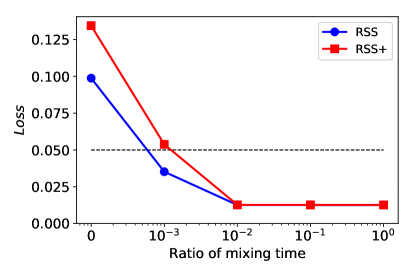
Figure 1: Loss of RSS and RSS+ as a function of the ratio of the theoretical mixing time.

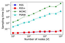
(a) $k=3$

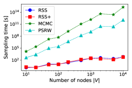
(b) $k=4$

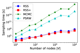
(c) $k=5$

Figure 2: Sampling Time (seconds) of MCMCSampling, PSRW, RSS and RSS+ for different size of BA graphs. Solid line shows actual sampling time, and dashed lines represents estimated time.

4.2 Sampling time comparison with BA graphs

We compare the sampling time, i.e., time to obtain one $k$-subgraph from the input graph, for MCMCSampling, PSRW, RSS, and RSS+.

Setting. We compare sampling times of each method for different size of graphs and different $k$. We fix the error $\varepsilon$ to $0.05$ and vary the size of the input graphs from $10^{1}$ to $10^{4}$. We also vary $k$ from 3 to 5. We measure the time to obtain one $k$-subgraph for each method for each setting 10 times, and report the averages. For small graphs and small $k$, we measure the actual time. For big graphs and for big $k$, we report the estimated time, based on the time taken to make 100 steps.

Dataset. We use Barabási-Albert (BA) model [2], which is a well-studied graph generating model of random scale-free networks using preferential attachment. The BA model parameter $m$ is set to 2. We vary $|V|$ from $10,20,50,...$ up to $10\,000$.

Results. The results are shown in Figure 2. Solid lines represent actual times and dashed lines represent estimated times. MCMCSampling and PSRW run slowly, e.g., for $|V|=100,k=5$ MCMCSampling takes $10^{10}$ seconds and PSRW takes $10^{7}$ seconds on the estimation.

RSS and RSS+ are both quite fast. For $k=3$, they run in almost constant time no matter how the size of the graph is big. Indeed, the theoretical running time of both RSS and RSS+ is $\mathcal{O}(1)$. For $k=4$ and $k=5$, the sampling time increases with $|V|$, however, compared to MCMCSampling and PSRW, the speed of the increase is mild. In addition, we confirm that RSS+ is faster than RSS, validating our theoretical results. The detailed comparison between RSS and RSS+ with higher $k$ can be found in Appendix B

5 Conclusion

In this paper, we have studied the problem of sampling $k$-subgraphs from a given graph. We have analyzed MCMCSampling, the standard MCMC approach for this problem, and PSRW, a state-of-the-art MCMC method. We improved the upper bounds for the mixing times for both methods, using the canonical-paths technique. In addition, we have proposed novel MCMC methods, RSS and RSS+, which sample $k$-subgraphs by sampling $(k-1)$-subgraphs in a recursive manner. We have derived the theoretical mixing time and the computational costs for the proposed methods. We performed experiments to compare RSS and RSS+ with the existing methods. We validated that RSS and RSS+ give uniform samples, and they are significantly faster than the existing methods.

Appendix

Appendix A Proofs

A.1 Lemma 3.1: Diameter of $k$-state graph $G^{(k)}$

The diameter of the $k$-state graph $G^{(k)}$ is at most $(D+k-1)$, where $D$ is the diameter of $G$.

Proof.

Consider distinct $x$ and $y$ in $G^{(k)}$, with $x=(V_{x},E_{x})$ and $y=(V_{y},E_{y})$.

If $V_{x}\cap V_{y}\neq\emptyset$, starting with $V_{x}$ as a current node set, we add one node in $V_{y}$ that is adjacent to the current node set, and remove one node from the current node set except for the nodes that have been added, so that the induced subgraph of $G$ with the current node set remains connected. This step corresponds to a one-step walk on $G^{(k)}$. After $(k-|V_{x}\cap V_{y}|)$ such steps we obtain a path from $x$ to $y$ on $G^{(k)}$. Thus, the length of the shortest path from $x$ to $y$ is at most $(k-|V_{x}\cap V_{y}|)\leq k$.

If $V_{x}\cap V_{y}=\emptyset$, we consider a shortest path from a node in $V_{x}$ to a node in $V_{y}$. The length of such a path is at most $D$. We add and remove nodes in the same manner as above; starting with $V_{x}$ as a current node set, we add one node from the path that is adjacent to the current node set, and remove one node from the set. Once we add all nodes in the path, i.e., after at most $D$ steps, the current node set contains one node in $V_{y}$. Then we add nodes from $V_{y}$ and remove one node from the set, as above. It takes $k-1$ steps until the set becomes equal to $V_{y}$. The total number of steps is at most $(D+k-1)$, which shows that the length of the corresponding walk from $x$ to $y$ is at most $(D+k-1)$.

Hence, for any choice of $x$ and $y$ in $V^{(k)}$, their distance on $G^{(k)}$ is at most $(D+k-1)$, and thus, the diameter of $G^{(k)}$ is at most $(D+k-1)$. ∎

A.2 Lemma 3.5: Mixing time of RSS+

The mixing time $t^{\prime}_{k}(\varepsilon)$ of the algorithm DegreePropSampling+($G,k,\varepsilon$) is $2k\Delta(k\ln|V|+3\ln k+\ln\Delta+\ln\varepsilon^{-1})=\mathcal{O}(k^{2}\Delta\ln|V|)$.

Proof.

We apply the canonical-paths argument to obtain a bound on the quantity $\overline{\rho}$, used in Inequality (1), for bounding the mixing time of the Markov chain. The set of states of this Markov chain is $\Omega=E^{(k-1)}$. The underlying graph is a complete graph with nodes $E^{(k-1)}$. The desired stationary distribution is $\pi_{x}=\frac{1}{Z}f(x)$, where $f(x)=d(v(x))/\binom{m(v(x))}{2}$, $v(x)$ is the corresponding node in $V^{(k)}$ whose node set is the union of nodes in $x$, $d(u)$ is the degree of $u$, and $m(u)$ is the number of $(k-1)$-subgraphs in $u$. We have

$$Z=\sum_{x\in\mathbb{E}^{(k-1)}}f(x)=\sum_{v\in V^{(k)}}d(v)=2|E^{(k)}|\leq k\Delta|V^{(k)}|.$$

Thus,

$$p(x,y)=\frac{1}{2|E_{k-1}|}\min\left\{1,\frac{f(y)}{f(x)}\right\},$$

and

$$Q(x,y) = \pi_{x}p(x,y)$$

$$= \frac{f(x)}{Z}\frac{1}{2|E_{k-1}|}\min\left\{1,\frac{f(y)}{f(x)}\right\}$$

$$= \frac{\min\{f(x),{f(y)}\}}{2Z|E_{k-1}|}.$$

We can now bound $\overline{\rho}$ as follows:

$$\overline{\rho} = \max_{(u,v)\in E_{k-1}\times E_{k-1}}\frac{1}{Q(u,v)}\sum_{\gamma_{xy}\ni(u,v)}\pi_{x}\pi_{y}|\gamma_{xy}|$$

$$= \max_{(u,v)\in E_{k-1}\times E_{k-1}}\frac{2Z|E_{k-1}|}{\min\{f(u),f(v)\}}\frac{f(u)}{Z}\frac{f(v)}{Z}$$

$$= 2\frac{|E_{k-1}|}{Z}\max_{(u,v)\in E_{k-1}\times E_{k-1}}\max\{f(u),f(v)\}$$

$$= 2\frac{|E_{k-1}|}{2|E_{k}|}\max_{u\in E_{k-1}}f(u)$$

$$\leq 2\max_{u\in V^{(k)}}d(u)$$

$$\leq 2k\Delta,$$

where we use the fact that $\frac{|E_{k-1}|}{2|E^{(k)}|}\leq 1$, when $k\ll|V|$. Hence, by Inequality (1), a bound on the mixing time $t^{\prime}_{k}(\varepsilon)$ can be obtained as follows:

$$t^{\prime}_{k}(\varepsilon) = \max_{x\in V^{(k)}}\tau_{x}(\varepsilon)$$

$$= \max_{x\in V^{(k)}}\overline{\rho}(\ln{\pi_{x}}^{-1}+\ln\varepsilon^{-1})$$

$$\leq 2k\Delta\max_{x\in V^{(k)}}(\ln\frac{Z}{f(x)}+\ln\varepsilon^{-1})$$

$$\leq 2k\Delta\max_{x\in V^{(k)}}(\ln\frac{k\Delta|V^{(k)}|\binom{m(v(x))}{2}}{d(v(x))}+\ln\varepsilon^{-1})$$

$$\leq 2k\Delta(\ln(k^{3}\Delta|V^{(k)}|)+\ln\varepsilon^{-1})$$

$$\leq 2k\Delta(3\ln k+\ln\Delta+k\ln|V|+\ln\varepsilon^{-1})$$

$$= \mathcal{O}(k^{2}\Delta\ln|V|).$$

∎

A.3 Lemma 3.7: Mixing time of PSRW

The mixing time of the algorithm PSRW is $\frac{1}{2}(k-1)!(k-1)\Delta^{k}(D+k-2)|V|((k-1)\ln|V|+\ln(k-1)+\ln\Delta+\ln\varepsilon^{-1})=\mathcal{O}((k-1)!(k-1)^{2}\Delta^{k}(D+k)|V|\ln|V|)$.

Proof.

We apply the canonical-paths technique to upper bound the mixing time. We consider a random walk on $G^{(k-1)}$. Note that we add a self-loop to each node with probability $\frac{1}{2}$ to avoid periodicity. The state space of the corresponding Markov chain is $V^{(k-1)}$. The stationary distribution is $\pi(x)=\frac{1}{Z}d(x)$, where $Z=\sum_{x\in V^{(k-1)}}d(x)=2|E^{(k-1)}|.$ The transition probability is $p(u,v)=\frac{1}{2d(u)}\geq\frac{1}{2\Delta_{k-1}},$ and $Q(u,v)=\pi(u)p(u,v)=\frac{1}{2Z}$. We choose as canonical path for $x$ to $y$ to be one of the shortest paths on $G^{(k-1)}$, hence $\gamma_{xy}\leq(D+k-2)$. The quality $\overline{\rho}$ is calculated as follows:

$$\overline{\rho} = \max_{(u,v)\in E^{(k-1)}}\frac{1}{Q(u,v)}\sum_{\gamma_{xy}\in\Gamma\wedge\gamma_{xy}\ni(u,v)}\pi(x)\pi(y)|\gamma_{xy}|$$

$$\leq \max_{(u,v)\in E^{(k-1)}}2Z\sum_{\gamma_{xy}\in\Gamma\wedge\gamma_{xy}\ni(u,v)}\frac{d(x)}{Z}\frac{d(x)}{Z}(D+k-2)$$

$$\leq 2\frac{{\Delta_{k-1}}^{2}}{Z}(D+k-2)\max_{(u,v)\in E^{(k-1)}}|\{\gamma_{xy}\in\Gamma\wedge\gamma_{xy}\ni(u,v)\}|$$

$$\leq 2\frac{(k-1)^{2}\Delta^{2}}{2|E^{(k-1)}|}(D+k-2)\left(\frac{|V^{(k-1)}|}{2}\right)^{2}$$

$$\leq \frac{1}{2}(k-1)^{2}\Delta^{2}(D+k-2)\frac{|V^{(k-1)}|}{2|E^{(k-1)}|}|V^{(k-1)}|$$

$$\leq \frac{1}{2}(k-1)!(k-1)\Delta^{k}(D+k-2)|V|.$$

Hence the mixing time $t_{k}^{\mathrm{PSRW}}$ of PSRW is bounded as follows:

$$t_{k}^{\mathrm{PSRW}} = \max_{x\in V^{(k-1)}}\tau_{x}(\varepsilon)$$

$$\leq \max_{x\in V^{(k-1)}}\overline{\rho}(\ln\pi(x)^{-1}+\varepsilon^{-1})$$

$$\leq \overline{\rho}(\ln(k-1)\Delta|V^{(k-1)}|+\varepsilon^{-1})$$

$$\leq \frac{1}{2}(k-1)!(k-1)\Delta^{k}(D+k-2)|V|(\ln(k-1)+\ln\Delta+(k-1)\ln|V|+\ln\varepsilon^{-1})$$

$$= \mathcal{O}((k-1)!(k-1)^{2}\Delta^{k}(D+k)|V|\ln|V|)$$

∎

A.4 Theorem 3.8: Computational cost of algorithm PSRW

The total computation cost of the algorithm PSRW is $\mathcal{O}(k!k(k-1)^{6}\Delta^{k+1}(D+k)|V|\ln|V|)$.

Proof.

As with MCMCSampling, each random-walk step of PSRW takes time $\mathcal{O}((k-1)^{4}\Delta)$. Hence, using Lemma 3.7, the computational cost of the random walk on $G^{(k-1)}$ is $\mathcal{O}((k-1)!(k-1)^{6}\Delta^{k+1}(D+k)|V|\ln|V|)$.

PSRW uses the same acceptance and rejection process as $\textsc{UniformSampling}(G,k,\varepsilon)$. PSRW takes one edge $(u,v)$ sampled from $E^{(k-1)}$ uniformly at random using the random walk on $G^{(k-1)}$. It accepts a $k$-subgraph whose node set is a union of nodes in $u$ and $v$ with probability $1/\binom{m}{2}$, where $m$ is the number of $(k-1)$-subgraphs in that $k$-subgraph, which is at most $k$. Hence, PSRW performs this step $\mathcal{O}(k^{2})$ times, in expectation, before it accepts. The computational cost of PSRW is $\mathcal{O}(k!k(k-1)^{6}\Delta^{k+1}(D+k)|V|\ln|V|)$. ∎

Appendix B Additional experiments

B.1 Sampling time difference between RSS and RSS+

We run RSS and RSS+ with higher $k$ to validate that RSS+ is faster than RSS.

Setting. We estimate the sampling times of RSS and RSS+ to obtain one subgraph from the same graph with different $k$. We set $k$ from 3 to 10 and set $\varepsilon$ to 0.05.

Dataset. We use the same BA graph with 100 nodes, which is the same graph used in the experiment 4.2. The BA model parameter $m$ is set to 2.

Results. The results are shown in Figure 3. For $k=3$ and $k=4$, the sampling time of RSS and RSS+ are almost the same. Indeed, the time complexities of RSS and RSS+ are the same, $\mathcal{O}(k^{2})$ for $k=3$ and $\mathcal{O}(k^{2}(k-1)^{2}\Delta\ln|V|)$ for $k=4$. When $k>4$, RSS+ runs faster compared to RSS, and the higher $k$ is, the larger the difference. For example, RSS+ is around 100 times faster than RSS at $k=8$, and 5000 times faster at $k=10$. Thus, we confirm that RSS+ is the fastest method among all methods we compared.

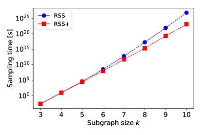
Figure 3: Sampling time of RSS and RSS+ as a function of $k$.

B.2 Mining patterns of Bitcoin Alpha web

As an application, we use RSS+ to mine local patterns in a real-world graph.

Setting. We run RSS+ to obtain 3- and 4-subgraphs and analyze the statistics to find interesting patterns. We set $\varepsilon=0.05$.

Dataset. We use the Bitcoin Alpha web of trust network [16, 15] available online from SNAP. This is a weighted signed directed graph whose nodes represent users of the Bitcoin Alpha platform. Edges represent rates of trust among users in a scale from $-10$ (total distrust) to $+10$ (total trust). The number of nodes, $|V|$, is $3\,783$, and the number of edges, $|E|$, is $24\,186$

Results. We run RSS+ on an undirected version of the graph, and after obtaining $k$-subgraphs we consider edge directions and weights. We obtain $10^{4}$ subgraphs, for $k=3$ and $4$. For memory efficiency and for speeding RSS+, we keep $G^{(3)}$ in memory.

The results are shown in Table 3. For $k=3$, we investigate the ratio of open triplets, triangles, and balanced triangles [12, 8]. A triangle is regarded as balanced if the number of negative edges among them is even. In this experiment, we consider that there exists a negative undirected edge between two nodes if there exists at least one negative directed edge, and if there are no negative directed edges and at least one positive directed edge among two nodes, we consider there exists an positive edge. For $k=4$, we calculate the ratio that the 4-subgraph is line-shaped, i.e., four nodes are connected only by one single path with three edges, and the ratio that the subgraph is a clique. The triangles in the graph are often balanced, and this shows that there exists some local mechanisms about the rating. It is also interesting that almost 93% of 4-subgraphs are line-shaped, and only 0.037% of the 4-subgraphs is a clique, showing that the local interactions among users are not active. One can also use our techniques to analyze other interesting local structures, for example, considering edge directions and edge weights, however, such an analysis is beyond the scope of this paper.

Table 3: Statistics of patterns of Bitcoin Alpha web

	Pattern	Ratio over all samples
$k=3$	open triplets	0.97190
	triangles	0.02810
	balanced triangles	0.02337
$k=4$	line-shaped	0.92798
	clique	0.00037

B.3 Motif statistics on a Barabási-Albert graph with 1 million nodes

To test the scalability of the proposed method, RSS+, we test it on a Barabási-Albert (BA) graph with one million nodes.

Setting. We run RSS+ on a graph with one million nodes, and obtain 1 000 samples. We set $k$ to 4, and $\varepsilon$ to 0.05. We count the frequency of motifs, i.e., small graphs with particular structures, and check how the frequency converges with the number of steps in the random walk.

Dataset. We generate a BA graph with 1 million nodes, setting the parameter $m$ to 2, thus the number of edges is around 2 millions.

Results. There are six 4-node motifs, however, only two motifs appear in the vast majority of our samples; the other four motifs appear very rarely. This is an effect of the specific structure of the BA graph. For instance, we see that our BA graph has very few triangles. The two motifs that appear in our samples, $M_{1}$ and $M_{2}$, are shown in Figure 4.

In Figure 5 we show the frequencies of $M_{1}$ and $M_{2}$ as a function of the length of random walk. It is interesting to observe that the motif frequencies converge with after 10 steps of the random walk, while the theoretical bound of the mixing time is $8.6\times 10^{5}$. Hence, our methods are useful for large graphs by setting appropriate length of random walks, which in practice can be much lower than the theoretical upper bounds.

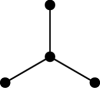
(a) motif $M_{1}$

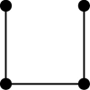
(b) motif $M_{2}$

Figure 4: The two most frequent motifs sampled in a Barabási-Albert (BA) graph. The other four motifs have very low frequencies (less than 1%).

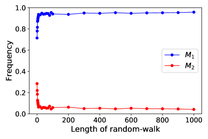
Figure 5: Motif frequencies of $M_{1}$ and $M_{2}$ as a function of the length of the random walk. The input graph is a BA graph with 1 million nodes.

References

- [1] N. K. Ahmed, J. Neville, R. A. Rossi, and N. Duffield, Efficient graphlet counting for large networks, in IEEE International Conference on Data Mining, 2015, pp. 1–10.
- [2] R. Albert and A.-L. Barabási, Statistical mechanics of complex networks, Reviews of modern physics, 74 (2002), pp. 47–97.
- [3] N. Alon, R. Yuster, and U. Zwick, Color-coding, Journal of the ACM, 42 (1995).
- [4] M. A. Bhuiyan, M. Rahman, M. Rahman, and M. Al Hasan, Guise: Uniform sampling of graphlets for large graph analysis, in IEEE International Conference on Data Mining, 2012, pp. 91–100.
- [5] M. A. Bhuiyan, M. Rahman, M. Rahman, and M. A. Hasan, Guise: Uniform sampling ofgraphlets for large graph analysis, IEEE International Conference on Data Mining, (2012).
- [6] I. Bordino, D. Donato, A. Gionis, and S. Leonardi, Mining large networks with subgraph counting, in IEEE International Conference on Data Mining, 2008, pp. 737–742.
- [7] M. Bressan, F. Chierichetti, R. Kumar, S. Leucci, and A. Panconesi, Motif counting beyond five nodes, ACM Transactions on Knowledge Discovery from Data, 12 (2018), pp. 1–25.
- [8] D. Cartwright and F. Harary, Structural balance: a generalization of heider’s theory, Psychological review, 63 (1956), p. 277.
- [9] J. Chen, W. Hsu, M. L. Lee, and S.-K. Ng, Nemofinder: Dissecting genome-wide protein-protein interactions with meso-scale network motifs, in ACM SIGKDD, 2006, pp. 106–115.
- [10] G. Han and H. Sethu, Waddling random walk: Fast and accurate mining of motif statistics in large graphs, in IEEE International Conference on Data Mining, 2016, pp. 181–190.
- [11] W. K. Hastings, Monte Carlo sampling methods using Markov chains and their applications, Biometrika, 57 (1970), pp. 97–109.
- [12] F. Heider, Attitudes and cognitive organization, The Journal of psychology, 21 (1946), pp. 107–112.
- [13] M. Jerrum and A. Sinclair, The Markov chain Monte Carlo method: an approach to approximate counting and integration, in Approximation algorithms for NP-hard problems, 1996.
- [14] M. Jha, C. Seshadhri, and A. Pinar, Path sampling: A fast and provable method for estimating 4-vertex subgraph counts, in International Conference on World Wide Web, 2015, pp. 495–505.
- [15] S. Kumar, B. Hooi, D. Makhija, M. Kumar, C. Faloutsos, and V. Subrahmanian, Rev2: Fraudulent user prediction in rating platforms, in ACM WSDM, 2018, pp. 333–341.
- [16] S. Kumar, F. Spezzano, V. Subrahmanian, and C. Faloutsos, Edge weight prediction in weighted signed networks, in IEEE International Conference on Data Mining, 2016, pp. 221–230.
- [17] J. Kunegis, A. Lommatzsch, and C. Bauckhage, The slashdot zoo: mining a social network with negative edges, in International Conference on World Wide Web, 2009, pp. 741–750.
- [18] H. Kwak, C. Lee, H. Park, and S. Moon, What is twitter, a social network or a news media?, in International Conference on World Wide Web, 2010, pp. 591–600.
- [19] X. Lu and S. Bressan, Sampling connected induced subgraphs uniformly at random, Scientific and Statistical Database Management, (2012), pp. 195–212.
- [20] N. Metropolis, A. W. Rosenbluth, M. N. Rosenbluth, A. H. Teller, and E. Teller, Equation of state calculations by fast computing machines, The journal of chemical physics, 21 (1953), pp. 1087–1092.
- [21] R. Milo, S. Shen-Orr, S. Itzkovitz, N. Kashtan, D. Chklovskii, and U. Alon, Network motifs: simple building blocks of complex networks, Science, 298 (2002), pp. 824–827.
- [22] A. Pinar, C. Seshadhri, and V. Vishal, Escape: Efficiently counting all 5-vertex subgraphs, in International Conference on World Wide Web, 2017, pp. 1431–1440.
- [23] A. Sinclair, Improved bounds for mixing rates of Markov chains and multicommodity flow, Combinatorics, Probability & Computing, (1992), pp. 351–370.
- [24] R. Toivonen, J.-P. Onnela, J. Saramäki, J. Hyvönen, and K. Kaski, A model for social networks, Physica A: Statistical Mechanics and its Applications, 371 (2006), pp. 851–860.
- [25] P. Wang, J. Lui, B. Ribeiro, D. Towsley, J. Zhao, and X. Guan, Efficiently estimating motif statistics of large networks, ACM Transactions on Knowledge Discovery from Data, 9 (2014), p. 8.
- [26] P. Wang, J. C. S. Lui, B. Ribeiro, D. Towsley, J. Zhao, and X. Guan, Efficiently estimating motif statistics of large networks, ACM Transactions on Knowledge Discovery from Data, 9 (2014).
- [27] P. Wang, J. Zhao, X. Zhang, Z. Li, J. Cheng, J. C. Lui, D. Towsley, J. Tao, and X. Guan, Moss-5: A fast method of approximating counts of 5-node graphlets in large graphs, IEEE Transactions on Knowledge and Data Engineering, 30 (2017), pp. 73–86.
- [28] W. Zachary, An information flow model for conflict and fission in small groups, Journal of Anthropological Research, 33 (1977), pp. 452–473.
- [29] J. Zhao, J. C. Lui, D. Towsley, X. Guan, and Y. Zhou, Empirical analysis of the evolution of follower network: A case study on Douban, in INFOCOM workshops, 2011, pp. 924–929.