On a Nadaraya-Watson Estimator with Two Bandwidths

Abstract

In a regression model, we write the Nadaraya-Watson estimator of the regression function as the quotient of two kernel estimators, and propose a bandwidth selection method for both the numerator and the denominator. We prove risk bounds for both data driven estimators and for the resulting ratio. The simulation study confirms that both estimators have good performances, compared to the ones obtained by cross-validation selection of the bandwidth. However, unexpectedly, the single-bandwidth cross-validation estimator is found to be much better than the ratio of the previous two good estimators, in the small noise context. However, the two methods have similar performances in models with large noise.

and

1 Introduction

Consider $n\in\mathbb{N}\backslash\{0\}$ independent random variables $X_{1},\dots,X_{n}$ having the same probability density $f$ with respect to Lebesgue’s measure. Consider also the random variables $Y_{1},\dots,Y_{n}$ defined by

$$Y_{i}=b(X_{i})+\varepsilon_{i}\textrm{ $;$ }i\in\{1,\dots,n\},$$

where $b$ is a measurable function from $\mathbb{R}$ into itself and $\varepsilon_{1},\dots,\varepsilon_{n}$ are $n$ i.i.d. centered random variables with variance $\sigma^{2}>0$ and independent of $X_{1},\dots,X_{n}$.
Since Nadaraya [15] and Watson [20], a lot of consideration has been given to the estimator of $b$ defined by

$$\widehat{b}_{n,h}(x):=\frac{\sum_{i=1}^{n}K\left(\frac{X_{i}-x}{h}\right)Y_{i}}{\sum_{i=1}^{n}K\left(\frac{X_{i}-x}{h}\right)}\textrm{ $;$ }x\in\mathbb{R},$$

where $K:\mathbb{R}\rightarrow\mathbb{R}$ is a kernel, and $h>0$ is the bandwidth. This estimator has been dealt with as a weighted estimator, for $K\geqslant 0$:

$$\widehat{b}_{n,h}(x)=\sum_{i=1}^{n}w_{n,h}^{(i)}(x)Y_{i},\quad w_{n,h}^{(i)}(x)=\frac{K\left(\frac{X_{i}-x}{h}\right)}{\sum_{i=1}^{n}K\left(\frac{X_{k}-x}{h}\right)},$$

and is often called ”local average regression”. It is studied e.g. in Jones and Wand [11], Györfi et al. [8] or defined in Tsybakov [19]. Recent papers still propose methods to improve the estimation, see Chang et al. [3]. Several strategies have been proposed to select the bandwidth in a data driven way. Cross-validation based on leave-one-out principle is one of the most standard methods to perform this choice (see Györfi et al. [8]), even if a lot of refinements have been proposed. Optimal rates depend on the regularity of the function $b$ and have been first established by Stone [18]: roughly speaking, they are of order $O(n^{-p/(2p+1)})$ for $b$ admitting $p$ derivatives. From theoretical point of view, the rates of the adaptive final estimator are not always given, nor proved.
In this paper, we re-write the Nadaraya-Watson as the quotient of two estimators, an estimator of $bf$ divided by an estimator of $f$:

$$\widehat{bf}_{n,h}(x):=\frac{1}{nh}\sum_{i=1}^{n}K\left(\frac{X_{i}-x}{h}\right)Y_{i}$$

and

$$\widehat{f}_{n,h^{\prime}}(x):=\frac{1}{nh^{\prime}}\sum_{i=1}^{n}K\left(\frac{X_{i}-x}{h^{\prime}}\right).$$

Clearly, $\widehat{f}_{n,h^{\prime}}$ is the Parzen-Rosenblatt estimator of $f$ (see Rosenblatt [17] and Parzen [16]). The question we are interested in is the following one: can we choose separately the two bandwidths in an adaptive way and obtain good performance for each, and then for the ratio? This is why we study the estimator

$$\widehat{b}_{n,h,h^{\prime}}(x):=\frac{\widehat{bf}_{n,h}(x)}{\widehat{f}_{n,h^{\prime}}(x)}\textrm{ $;$ }x\in\mathbb{R}$$

as an estimator of the regression function $b$, where $h,h^{\prime}>0$ and $K:\mathbb{R}\rightarrow\mathbb{R}$ is a (not necessarily nonnegative) kernel. Thus, $\widehat{b}_{n,h,h}=\widehat{b}_{n,h}$ is the initial Nadaraya-Watson estimator of $b$ with single bandwidth $h$. For this reason, the estimator studied in this paper is called the two bandwidths Nadaraya-Watson (2bNW) estimator.
Adaptive estimation of the density has been widely studied recently. A bandwidth selection method has been proposed by Goldenschluger and Lepski [7], and proved to reach the adequate bias-variance compromise. Implementation of this method revealed to be difficult due to the choice of two constants involved in the procedure, the intuition of which is not obvious. This is why the question was further investigated by Lacour et al. [13]: they improve and modify the strategy by using specific theoretical tools for their proofs. Precisely, thanks to a deviation inequality for U-statistics proved by Houdré and Reynaud-Bouret [10], they bound the Mean Integrated Square Error of their final estimator, which they call PCO (Penalised Comparison to Overfitting) estimator. Numerically, the good performance of their proposal has been illustrated in a naive way and for high order kernels in Comte and Marie [5], and through a systematic numerical study in Lacour et al. [14], including the multivariate case. These two methods and the associated results are dedicated to the selection of $h^{\prime}$ for $\widehat{f}_{n,h^{\prime}}(x)$, and we can use them. Unfortunately, the theoretical results do not apply to $\widehat{bf}_{n,h}(x)$, mainly because they hold under a boundedness assumption: in our context, this would lead to assume that the $Y_{i}$’s are bounded. We do not want to require such an assumption as it would exclude the case of Gaussian errors $\varepsilon_{i}$, for instance. Thus, we give moment assumptions under which the Goldenshluger and Lepski method on the one hand (see Section 3) and the PCO estimator on the other hand (see Section 4) can be applied to the estimation of $bf$. When gathering the results for the numerator and the denominator, we can bound the risk of the quotient estimator of $b$.
Concretely, we implement the PCO method for $bf$ and compare it with a cross-validation (CV) strategy: in our examples, PCO almost always performs slightly better than CV. Therefore, the PCO adaptive estimation strategies for $f$ and for $bf$ are clearly good. However, unexpectedly, for small noise ($\sigma=0.1$), the quotient fails systematically to beat the specific regression CV method. Even if we compare the classical single-bandwidth CV regression estimator to the ratio of the oracles estimators of the numerator and the denominator, the former wins, and we obtain a quotient with two bandwidths which is in mean much less good than the CV estimator with single bandwidth. In practice, the bandwidth selected by the CV algorithm in that case is very small, and associated to quite bad estimators of the numerator and of the denominator. This remark is of important interest for practitioners. In a second time, we increased the noise ($\sigma=0.7$), and finally obtained results indicating that the two methods can have similar Mean Integrated Squared Errors (MISE) in this more difficult context. This, together with the fact we establish a theoretical risk bound on the PCO adaptive 2bNW estimator, imply that the PCO method, for both numerator and denominator, remains an interesting bandwidth selection method. Moreover, we believe that both positive but also negative results are of interest, and detailed tables, explanations and discussion are given in Section 5.

Notations:

1. For every square integrable functions $f,g:\mathbb{R}\rightarrow\mathbb{R}$,

   $$(f\ast g)(x):=\int_{-\infty}^{\infty}f(x-y)g(y)dy\textrm{ $;$ }x\in\mathbb{R}.$$

2. $K_{\varepsilon}:=1/\varepsilon K(\cdot/\varepsilon)$ for every $\varepsilon>0$.

2 Bound on the MISE of the 2bNW estimator

First, we state some simple risk bound results in the case of a fixed bandwidth.

Consider $\beta>0$ and $\ell:=\lfloor\beta\rfloor$, where $\lfloor\beta\rfloor$ denotes the largest integer smaller than $\beta$. In the sequel, the kernel $K$ and the density function $f$ fulfill the following assumption.

Assumption 2.1.

 

• The map $K$ belongs to $\mathbb{L}^{2}(\mathbb{R},dy)$, $K$ is bounded and $\int_{{\mathbb{R}}}K(y)dy=1$.

• The density function $f$ is bounded.

Under this assumption, a suitable control of the MISE of $\widehat{bf}_{n,h}$ has been established in Comte [4], Proposition 4.2.1.

Proposition 2.2.

Under Assumption 2.1,

$$\mathbb{E}(\|\widehat{bf}_{n,h}-bf\|_{2}^{2})\leqslant\|bf-(bf)_{h}\|_{2}^{2}+\frac{\mathfrak{c}_{K,Y}}{nh}$$

where $(bf)_{h}:=K_{h}\ast(bf)$ and $\mathfrak{c}_{K,Y}:=\|K\|_{2}^{2}\mathbb{E}(Y_{1}^{2})$.

In order to provide a suitable control on the MISE of the 2bNW estimator, we assume that $b$ and $f$ fulfill the following assumption.

Assumption 2.3.

The function $b^{2}f$ is bounded by a constant $\mathfrak{c}_{b,f}>0$.

Note that this assumption does not require that $b$ is bounded and is satisfied in most classical examples.
Moreover, for any $\mathcal{S}\in\mathcal{B}(\mathbb{R})$, consider the norm $\|.\|_{2,f,\mathcal{S}}$ on $\mathbb{L}^{2}(\mathcal{S},f(x)dx)$ defined by

$$\|\varphi\|_{2,f,\mathcal{S}}:=\left(\int_{\mathcal{S}}\varphi(x)^{2}f(x)dx\right)^{1/2}\textrm{$;$ }\forall\varphi\in\mathbb{L}^{2}(\mathcal{S},f(x)dx).$$

Proposition 2.4.

Let $m_{n}$ be a positive real number and consider

$$\mathcal{S}_{n}:=\{x\in\mathbb{R}:f(x)\geqslant m_{n}\}.$$

Under Assumptions 2.1 and 2.3,

$$\mathbb{E}(\|\widehat{b}_{n,h,h^{\prime}}-b\|_{2,f,\mathcal{S}_{n}}^{2})\leqslant\frac{8\mathfrak{c}_{f}}{m_{n}^{2}}\left(\|bf-(bf)_{h}\|_{2}^{2}+\frac{\mathfrak{c}_{K,Y}}{nh}+2\mathfrak{c}_{b,f}\left(\|f-f_{h^{\prime}}\|_{2}^{2}+\frac{\mathfrak{c}_{K}}{nh^{\prime}}\right)\right)$$

where $(bf)_{h}:=K_{h}\ast(bf)$, $f_{h^{\prime}}=K_{h^{\prime}}\ast f$, $\mathfrak{c}_{f}:=\|f\|_{\infty}^{2}\vee 1$ and $\mathfrak{c}_{K}:=\int_{{\mathbb{R}}}K(y)^{2}dy.$

The idea behind Proposition 2.4 is that we cannot pretend to accurately estimate $b$ on domains where few $X_{i}$’s are observed. Such domains correspond to small level of the density. For small $m_{n}$, the set ${\mathcal{S}}_{n}$ excludes these cases.
Proposition 2.4 gives a decomposition of the risk of the quotient estimator as the sum of the risks of the estimators of the numerator $bf$ and of the denominator $f$, up to the multiplicative constant $8\mathfrak{c}_{f}/m_{n}^{2}$. Therefore, the rate of the quotient estimator is, in the best case, the worst rate of the two estimators used to define it (see also Remark 2.5 below). The factor $1/m_{n}^{2}$ may imply a global loss with respect to this rate. Clearly, the smaller is $m_{n}$, the larger is the loss.
For instance, if $f$ is lower bounded by a known constant $f_{0}$ on a given compact set $A$, then we can take ${\mathcal{S}}_{n}=A$ and $m_{n}=f_{0}$. In that case, no loss occurs. If $f_{0}$ is unknown, we still can bound the risk with ${\mathcal{S}}_{n}=A$ and $1/m_{n}^{2}=\log(n)$ for $n$ large enough. A log-loss occurs then in the rate.

Remark 2.5.

We consider, for $\beta,L>0$, the Nikol’ski ball ${\mathcal{H}}(\beta,L)$, defined as the set of $\ell=\lfloor\beta\rfloor$ times continuously derivable functions $\varphi:\mathbb{R}\rightarrow\mathbb{R}$ such that $\varphi^{(\ell)}$ satisfies

$$\left[\int_{-\infty}^{\infty}(\varphi^{(\ell)}(x+t)-\varphi^{(\ell)}(x))^{2}dx\right]^{1/2}\leqslant L|t|^{\beta-\ell}\textrm{ $;$ }\forall t\in\mathbb{R}.$$

For instance, for $p\in\mathbb{N}$, any function $\varphi\in C^{p+1}(\mathbb{R})$ such that ${\rm supp}(\varphi^{(p)})=[0,1]$ and $\|\varphi^{(p+1)}\|_{\infty}\leqslant L$ belongs to $\mathcal{H}(p+1,L)$. Indeed, for every $t\in\mathbb{R}_{+}$,

$$\int_{-\infty}^{\infty}(\varphi^{(p)}(x+t)-\varphi^{(p)}(x))^{2}dx \leqslant t\int_{-t}^{1}\int_{x}^{x+t}\varphi^{(p+1)}(z)^{2}\mathbf{1}_{[0,1]}(z)dzdx$$

$$\leqslant L^{2}t\int_{-t}^{1}((x+t)\wedge 1-x\vee 0)dx$$

$$= L^{2}t\left(\int_{0}^{1+t}(x\wedge 1)dx-\int_{0}^{1}xdx\right)=L^{2}t^{2}.$$

More subtly, $\psi:x\mapsto e^{-x}\mathbf{1}_{\mathbb{R}_{+}}(x)$ belongs to $\mathcal{H}(1/2,1)$. Indeed, for every $t\in\mathbb{R}_{+}$,

$$\int_{-\infty}^{\infty}(\psi(x+t)-\psi(x))^{2}dx = \int_{-t}^{\infty}e^{-2(x+t)}dx-2\int_{0}^{\infty}e^{-t-2x}dx+\int_{0}^{\infty}e^{-2x}dx$$

$$= \lim_{x\rightarrow\infty}-\frac{1}{2}[e^{-2t}(e^{-2x}-e^{2t})-2e^{-t}(e^{-2x}-1)$$

$$\hskip 85.35826pt+e^{-2x}-1]=1-e^{-t}\leqslant t.$$

Now, assume that $bf$ belongs to $\mathcal{H}(\beta_{1},L)$ and $f$ to $\mathcal{H}(\beta_{2},L)$. We also assume that the kernel $K$ satisfies Assumption 2.1 and is of order $\ell=\lfloor\max(\beta_{1},\beta_{2})\rfloor$, that is

$$\int_{-\infty}^{\infty}|u^{k}K(u)|du<\infty\quad\textrm{and}\quad\int_{-\infty}^{\infty}u^{k}K(u)du=0\textrm{ $;$ }\forall k\in\{1,\dots,\ell\}.$$

Then, it follows from Tsybakov [19], Chapter 1, that

$$\|bf-(bf)_{h}\|_{2}^{2}\leqslant C(\beta_{1},L)h^{2\beta_{1}}\quad\textrm{and}\quad\|f-f_{h^{\prime}}\|_{2}^{2}\leqslant C^{\prime}(\beta_{2},L)(h^{\prime})^{2\beta_{2}}.$$

This implies that choosing $h_{{\rm opt}}=c_{1}n^{1/(2\beta_{1}+1)}$ in Proposition 2.2 yields

$$\mathbb{E}(\|\widehat{bf}_{n,h_{\rm opt}}-bf\|_{2}^{2})\lesssim n^{-2\beta_{1}/(2\beta_{1}+1)},$$

which is a standard optimal rate of estimation on Nikol’ski balls. The same rate holds for the estimation of $f$ under our assumptions, with $\beta_{1}$ replaced by $\beta_{2}$, and $h_{\rm opt}^{\prime}=c_{2}n^{1/(2\beta_{2}+1)}$. This implies that

$$\|bf-(bf)_{h_{\rm opt}}\|_{2}^{2}+\frac{\mathfrak{c}_{K,Y}}{nh_{\rm opt}}+2\mathfrak{c}_{b,f}\left(\|f-f_{h_{\rm opt}^{\prime}}\|_{2}^{2}+\frac{\mathfrak{c}_{K}}{nh_{\rm opt}^{\prime}}\right)$$

$$\hskip 142.26378pt\lesssim\max(n^{-2\beta_{1}/(2\beta_{1}+1)},n^{-2\beta_{2}/(2\beta_{2}+1)}).$$

So, the rate is optimal if $\beta=\min(\beta_{1},\beta_{2})$ is the regularity of $b$.
However, such bandwidth choices are not possible in practice, as they depend on unknown regularity parameters. Data driven bandwidth selection methods are settled to automatically reach a squared bias-variance compromise, inducing the optimal rate if the function under estimation does belong to a regularity space.

3 A bandwidth selection procedure for the 2bNW estimator based on the GL method

The bound on the MISE of $\widehat{b}_{n,h,h^{\prime}}$ obtained in Proposition 2.4 suggests to select $h$ and $h^{\prime}$ separately, so that both bounds are minimal. The Goldenshluger-Lepski method (see Goldenshluger and Lepski [7]) allows to do this for $\widehat{f}_{n,h^{\prime}}$, but requires to be extended to the estimator of $bf$. In particular, extensions of the proof are required as we do not wish to assume that the $Y_{i}$’s are bounded.

Consider the collection of bandwidths $\mathcal{H}_{n}:=\{h_{1},\dots,h_{N(n)}\}\subset[0,1]$, where $N(n)\in\{1,\dots,n\}$ and

$$\frac{1}{n}<h_{1}<\dots<h_{N(n)}.$$

Moreover, we will need the following conditions.

Assumption 3.1.

There exists $\mathfrak{m}>0$, not depending on $n$, such that

$$\frac{1}{n}\sum_{i=1}^{N(n)}\frac{1}{h_{i}}\leqslant\mathfrak{m},$$

and for every $c>0$, there exists $\mathfrak{m}(c)>0$, not depending on $n$, such that

$$\sum_{i=1}^{N(n)}\frac{1}{\sqrt{h_{i}}}\exp\left(-\frac{c}{\sqrt{h_{i}}}\right)\leqslant\mathfrak{m}(c).$$

Example. Consider the dyadic bandwidths defined by

$$h_{i}:=2^{-i}\textrm{ $;$ }\forall i=0,1,\dots,\left[\frac{\log(n)}{\log(2)}\right].$$

Then,

$$\frac{1}{n}\sum_{i=1}^{[\log(n)/\log(2)]}2^{i}\leqslant\frac{2n-1}{n}\leqslant 2$$

and

$$\sum_{i=1}^{[\log(n)/\log(2)]}2^{i/2}\exp(-c2^{i/2})\leqslant\sum_{i=1}^{n}\sqrt{i}\exp(-c\sqrt{i})\leqslant\mathfrak{m}(c)<\infty.$$

Thus, Assumption 3.1 is fulfilled.

Consider also

$$\widehat{bf}_{n,h,\eta}(x) := (K_{\eta}\ast\widehat{bf}_{n,h})(x)$$

$$= \frac{1}{n}\sum_{i=1}^{n}Y_{i}(K_{\eta}\ast K_{h})(X_{i}-x).$$

We apply the Goldenshluger-Lepski bandwidth selection method to $\widehat{bf}_{n,h}$ by solving the minimization problem

$$\min_{h\in\mathcal{H}_{n}}\{A_{n}(h)+V_{n}(h)\}$$ (1)

where

$$A_{n}(h):=\sup_{\eta\in\mathcal{H}_{n}}(\|\widehat{bf}_{n,h,\eta}-\widehat{bf}_{n,\eta}\|_{2}^{2}-V_{n}(\eta))_{+}\quad\textrm{ and }\quad V_{n}(h):=\upsilon\frac{\mathfrak{c}_{K,Y}}{nh}\|K\|_{1}^{2},$$

with $\upsilon>0$ not depending on $n$ and $h$, and $\mathfrak{c}_{K,Y}=\|K\|_{2}^{2}\mathbb{E}(Y_{1}^{2})$. In the sequel, the solution to the minimization Problem (1) is denoted by $\widehat{h}_{n}$.
The idea behind the criterion is that $A_{n}(h)$ is an estimate of the squared bias term $\|(bf)_{h}-bf\|_{2}^{2}$ and $V_{n}(h)$ an estimate of the variance. So, $\widehat{h}_{n}$ makes the compromise. See more details about the heuristics in Chagny [2], Section 4.4.

Theorem 3.2.

Under Assumptions 2.1 and 3.1, if $\mathbb{E}(Y_{1}^{6})<\infty$, then there exist two deterministic constants $\mathfrak{c},\overline{\mathfrak{c}}>0$, not depending on $n$, such that

$$\mathbb{E}(\|\widehat{bf}_{n,\widehat{h}_{n}}-bf\|_{2}^{2})\leqslant\mathfrak{c}\cdot\inf_{h\in\mathcal{H}_{n}}\{\|(bf)_{h}-bf\|_{2}^{2}+V_{n}(h)\}+\overline{\mathfrak{c}}\frac{\log(n)^{2}}{n}.$$

Theorem 3.2 states that $\widehat{bf}_{n,\widehat{h}_{n}}$ automatically leads to a compromise between the squared bias ($\|(bf)_{h}-bf\|_{2}^{2}$) and the variance ($V_{n}(h)$) terms. The multiplicative constant $\mathfrak{c}$, which is larger than one, is the price of the method but preserves the rate. Lastly, the additive quantity $\overline{\mathfrak{c}}\log(n)^{2}/n$ is negligible with respect to the possible rate of convergence (see Remark 2.5).
We recall now a version of the result proved by Goldenshluger and Lepski [7], which is available for the estimator of $f$. See also a simplified proof in Comte [4], Section 4.2. Let us consider

$$\widehat{h}_{n}^{\prime}\in\arg\min_{h^{\prime}\in\mathcal{H}_{n}}\{A_{n}^{\prime}(h^{\prime})+V_{n}^{\prime}(h^{\prime})\},$$

where

$$A_{n}^{\prime}(h^{\prime}):=\sup_{\eta\in\mathcal{H}_{n}}(\|K_{\eta}\ast\widehat{f}_{n,h^{\prime}}-\widehat{f}_{n,\eta}\|_{2}^{2}-V_{n}^{\prime}(\eta))_{+}\quad\textrm{and}\quad V_{n}^{\prime}(h^{\prime}):=\chi\frac{\|K\|_{2}^{2}\|K\|_{1}^{2}}{nh^{\prime}}$$

with $\chi>0$ not depending on $n$ and $h^{\prime}$. Under Assumptions 2.1 and 3.1, there exist two deterministic constants $\mathfrak{c}^{\prime},\overline{\mathfrak{c}}^{\prime}>0$, not depending on $n$, such that

$$\mathbb{E}(\|\widehat{f}_{n,\widehat{h}_{n}^{\prime}}-f\|_{2}^{2})\leqslant\mathfrak{c}^{\prime}\cdot\inf_{h^{\prime}\in\mathcal{H}_{n}}\{\|f_{h^{\prime}}-f\|_{2}^{2}+V_{n}^{\prime}(h^{\prime})\}+\frac{\overline{\mathfrak{c}}^{\prime}}{n}$$ (2)

Gathering (2) and Theorem 3.2 yields a Corollary similar to Proposition 2.4.

Corollary 3.3.

Let $m_{n}$ be a positive real number and consider

$$\mathcal{S}_{n}:=\{x\in\mathbb{R}:f(x)\geqslant m_{n}\}.$$

Under Assumptions 2.1, 2.3 and 3.1, if $\mathbb{E}(Y_{1}^{6})<\infty$, then

$$\mathbb{E}(\|\widehat{b}_{n,\widehat{h}_{n},\widehat{h}_{n}^{\prime}}-b\|_{2,f,\mathcal{S}_{n}}^{2}) \leqslant \mathfrak{C}_{n}\inf_{(h,h^{\prime})\in\mathcal{H}_{n}^{2}}\{\|(bf)_{h}-bf\|_{2}^{2}+\|f_{h^{\prime}}-f\|_{2}^{2}$$

$$\hskip 56.9055pt+V_{n}(h)+V_{n}^{\prime}(h^{\prime})\}+\overline{\mathfrak{C}}_{n}\frac{\log(n)^{2}}{n},$$

where

$$\mathfrak{C}_{n}:=\frac{8\mathfrak{c}_{f}}{m_{n}^{2}}(\mathfrak{c}\vee(2\mathfrak{c}_{b,f}\mathfrak{c}^{\prime}))\quad\textrm{and}\quad\overline{\mathfrak{C}}_{n}:=\frac{8\mathfrak{c}_{f}}{m_{n}^{2}}(\overline{\mathfrak{c}}+2\mathfrak{c}_{b,f}\overline{\mathfrak{c}}^{\prime}).$$

The comments following Proposition 2.4 and in Remark 2.5 apply here.

4 A bandwidths selection procedure for the 2bNW estimator based on the PCO method

The Goldenshluger-Lepski method is mathematically very nice and provides a rigorous risk bound for the adaptive estimator with random bandwidth. However, it has been acknowledged as being difficult to implement, due to the square grid in $h,\eta$ required to compute intermediate versions of the criterion and to the lack of intuition to guide the choice of the constants $\upsilon$ and $\chi$ which should be calibrated from preliminary simulation experiments, see e.g. Comte and Rebafka [6]. This is the reason why Lacour et al. [13] investigated and proposed a simplified criterion (PCO) relying on deviation inequalities for $U$-statistics due to Houdré and Reynaud-Bouret [10]. This inequality applies in our more complicated context and Lacour-Massart-Rivoirard’s result can be extended here as follows.

Let us recall that $K_{h}(\cdot)=1/hK(\cdot/h)$ and

$$(bf)_{h}=\mathbb{E}(\widehat{bf}_{n,h})=K_{h}\ast(bf)$$

(see Lemma 6.1). Let $h_{\min}$ be the smallest bandwidth value in $\mathcal{H}_{n}$ and consider

$$\textrm{crit}(h):=\|\widehat{bf}_{n,h}-\widehat{bf}_{n,h_{\min}}\|_{2}^{2}+\textrm{pen}(h)$$

with

$$\textrm{pen}(h):=\frac{2\langle K_{h_{\min}},K_{h}\rangle_{2}}{n^{2}}\sum_{i=1}^{n}Y_{i}^{2}.$$

Then, let us define

$$\widetilde{h}_{n}\in\arg\min_{h\in\mathcal{H}_{n}}\textrm{crit}(h).$$

The idea behind the proposal of Lacour et al. (2017) is that, instead of comparing estimators $\widehat{bf}_{n,h}$ to a collection of estimators $\widehat{bf}_{n,h,\eta}$ for different bandwidths $\eta$, it is sufficient to compare them to the same single estimator, corresponding to the smallest bandwidth. See their Section 3.1 for more heuristic elements. This implies a faster and more efficient numerical procedure.
In the sequel, in addition to Assumption 2.1, the kernel $K$, the functions $b$ and $f$, the distribution of $Y_{1}$ and $h_{\min}$ fulfill the following assumption.

Assumption 4.1.

The kernel $K$ is symmetric and $K(0)>0$,

$$\frac{1}{nh_{\min}}\leqslant 1,$$

$bf$ is bounded, and there exists $\alpha>0$ such that $\mathbb{E}(\exp(\alpha|Y_{1}|))<\infty$.

As for Assumption 2.3, we can note that assuming $bf$ bounded does not require $b$ to be bounded, since most densities decrease fast at infinity. Moreover, the moment condition here is $\mathbb{E}(\exp(\alpha|Y_{1}|))<\infty$ and is stronger than for the Goldenschluger and Lepski method ($\mathbb{E}(Y_{1}^{6})<\infty$).

Theorem 4.2.

Consider $\vartheta\in(0,1)$. Under Assumptions 2.1 and 4.1, there exist two deterministic constants $\mathfrak{a},\mathfrak{b}>0$, not depending on $n$, $h_{\min}$ and $\vartheta$, such that

$$\mathbb{E}(\|\widehat{bf}_{n,\widetilde{h}_{n}}-bf\|_{2}^{2})\leqslant(1+\vartheta)\inf_{h\in\mathcal{H}_{n}}\mathbb{E}(\|\widehat{bf}_{n,h}-bf\|_{2}^{2})+\frac{\mathfrak{a}}{\vartheta}\|(bf)_{h_{\min}}-bf\|_{2}^{2}+\frac{\mathfrak{b}}{\vartheta}\cdot\frac{\log(n)^{5}}{n}.$$

Theorem 4.2 states that the estimator $\widehat{bf}_{n,\widetilde{h}_{n}}$ has performance of order of the best estimator of the collection $\inf_{h\in\mathcal{H}_{n}}\mathbb{E}(\|\widehat{bf}_{n,h}-bf\|_{2}^{2})$ up to a factor $(1+\vartheta)$. Indeed, the two other terms can be considered as negligible. If $bf$ is in the Nikol’ski ball ${\mathcal{H}}(\beta_{1},L)$ as in Remark 2.5, then the first right-hand-side term is of order $n^{-2\beta_{1}/(2\beta_{1}+1)}$. Since for $h_{\min}=1/n$, $\|(bf)_{h_{\min}}-bf\|_{2}^{2}$ is of order $n^{-2\beta_{1}}$, both this term and the last residual term $\log(n)^{5}/n$ are negligible compared to the first one.

Now, we state the result that can be deduced from Lacour et al. [13] for the estimator of $f$. Let us consider

$$\widetilde{h}_{n}^{\prime}\in\arg\min_{h^{\prime}\in\mathcal{H}_{n}}\textrm{crit}^{\prime}(h^{\prime}),$$

where

$$\textrm{crit}^{\prime}(h^{\prime}):=\|\widehat{f}_{n,h^{\prime}}-\widehat{f}_{n,h_{\min}}\|_{2}^{2}+\textrm{pen}^{\prime}(h^{\prime})\quad\textrm{and}\quad\textrm{pen}^{\prime}(h^{\prime}):=\frac{2\langle K_{h_{\min}},K_{h}\rangle_{2}}{n}.$$

By Lacour et al. [13], Theorem 2, there exists two deterministic constants $\mathfrak{a}^{\prime},\mathfrak{b}^{\prime}>0$, not depending on $n$ and $h_{\min}$, such that for every $\vartheta\in(0,1)$,

$$\mathbb{E}(\|\widehat{f}_{n,\widetilde{h}_{n}^{\prime}}-f\|_{2}^{2}) \leqslant (1+\vartheta)\inf_{h^{\prime}\in\mathcal{H}_{n}}\mathbb{E}(\|\widehat{f}_{n,h^{\prime}}-f\|_{2}^{2})+\frac{\mathfrak{a}^{\prime}}{\vartheta}\|f_{h_{\min}}-f\|_{2}^{2}+\frac{\mathfrak{b}^{\prime}}{\vartheta n}.$$

Again, we can gather this last result and Theorem 4.2 to get the following Corollary.

Corollary 4.3.

Let $m_{n}$ be a positive real number and consider

$$\mathcal{S}_{n}:=\{x\in\mathbb{R}:f(x)\geqslant m_{n}\}.$$

Consider also $\vartheta\in(0,1)$. Under Assumptions 2.1, 2.3 and 4.1,

$$\mathbb{E}(\|\widehat{bf}_{n,\widetilde{h}_{n},\widetilde{h}_{n}^{\prime}}-bf\|_{2,f,\mathcal{S}_{n}}^{2}) \leqslant (1+\vartheta)\mathfrak{C}_{n}(1,1)\inf_{(h,h^{\prime})\in\mathcal{H}_{n}^{2}}\{\mathbb{E}(\|\widehat{bf}_{n,h}-bf\|_{2}^{2})$$

$$\hskip 113.81102pt+\mathbb{E}(\|\widehat{f}_{n,h^{\prime}}-f\|_{2}^{2})\}$$

$$+\frac{\mathfrak{C}_{n}(\mathfrak{a},\mathfrak{a}^{\prime})}{\vartheta}(\|(bf)_{h_{\min}}-bf\|_{2}^{2}+\|f_{h_{\min}}-f\|_{2}^{2})$$

$$+\frac{\mathfrak{C}_{n}(\mathfrak{b},\mathfrak{b}^{\prime})}{\vartheta}\cdot\frac{\log(n)^{5}}{n},$$

where

$$\mathfrak{C}_{n}(u,v):=\frac{8\mathfrak{c}_{f}}{m_{n}^{2}}(u\vee(2\mathfrak{c}_{b,f}v))\textrm{ $;$ }\forall u,v\in\mathbb{R}.$$

The proof of Corollary 4.3 relies to the same arguments as the proof of Corollary 3.3 provided in Section 3.3, and is therefore omitted.

5 Simulation study

For the noise, we consider $\varepsilon\sim\sigma\mathcal{N}(0,1)$, with $\sigma=0.1$ and $\sigma=0.7$. For the signal, we take either $X\sim\mathcal{N}(0,1)$ or $X\sim\gamma(3,2)/5$ (where the factor $5$ is set to keep the variance of $X$ of order $1$, as in the first case). For the function $b$, we took functions with different features and regularities:

• $b_{1}(x)=\exp(-x^{2}/2)$,

• $b_{2}(x)=x^{2}/4-1$,

• $b_{3}(x)=\sin(\pi x)$,

• $b_{4}(x)=\exp(-|x|)$.

We illustrate in Figures 1 and 2 the difference between a sample generated with $\sigma=0.1$ (small noise) and with $\sigma=0.7$ (large noise), compared with the functions to estimate. We can see that the first case is easy and that the second one is very difficult. Notice that the vertical scales are different.

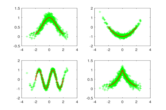
Figure 1: Observations $(X_{i},Y_{i})_{1\leqslant i\leqslant n}$ for $n=1000$ in the four cases of functions $b_{1}$ to $b_{4}$, with small noise $\sigma=0.1$, and true regression function in bold red.

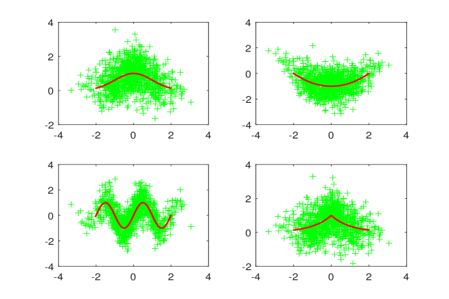
Figure 2: Observations $(X_{i},Y_{i})_{1\leqslant i\leqslant n}$ for $n=1000$ in the four cases of functions $b_{1}$ to $b_{4}$, with large noise $\sigma=0.7$, and true regression function in bold red.

5.1 Estimation of $bf$

The PCO method is implemented for $f$ and $bf$ with a kernel of order $7$ (i.e. $\int x^{k}K(x)dx=0$ for $k=1$ to $7$), defined by $K(x)=4n_{1}(x)-6n_{2}(x)+4n_{3}(x)-n_{4}(x)$, where $n_{j}(.)$ is a Gaussian density with mean $0$ and variance $j$. Note that, for $n_{j,h}(x):=1/hn_{j}(x/h)$, it holds that

$$\langle n_{i,h_{1}},n_{j,h_{2}}\rangle_{2}=\int_{-\infty}^{\infty}n_{i,h_{1}}(x)n_{j,h_{2}}(x)dx=\frac{1}{\sqrt{2\pi}}\times\frac{1}{\sqrt{ih_{1}^{2}+jh_{2}^{2}}}$$ (3)

The bandwidth is selected among $M=75$ equispaced values in between $0.01$ and $1$. All functions (true or estimated) are computed at 100 equispaced points in the interquantile interval corresponding to the $2\%$ and $98\%$ quantiles of $X$. The bandwidth is selected via the PCO criterion, where $h_{\rm min}=0.01$, and

$$\textrm{crit}(h):=\|\widehat{bf}_{n,h}-\widehat{bf}_{n,h_{\min}}\|_{2}^{2}+\textrm{pen}(h)\quad\textrm{with}\quad\textrm{pen}(h):=\frac{2\langle K_{h_{\min}},K_{h}\rangle_{2}}{n^{2}}\sum_{i=1}^{n}Y_{i}^{2}.$$

Note that the bandwidth of the density estimator is selected as in Comte and Marie [5], by minimizing

$$\textrm{crit}^{\prime}(h):=\|\widehat{f}_{n,h}-\widehat{f}_{n,h_{\min}}\|_{2}^{2}+2\textrm{pen}^{\prime}(h)\quad\textrm{with}\quad\textrm{pen}^{\prime}(h):=\frac{2\langle K_{h_{\min}},K_{h}\rangle_{2}}{n}.$$

The $\mathbb{L}^{2}$-norm is computed as a Riemann sum on the interquantile interval, while the penalty is explicit and exact, thanks to Formula (3).
The cross-validation (CV) criterion for selecting the bandwidth of $\widehat{bf}_{n,h}$ is computed as follows:

$$CV(h):=\int\widehat{bf}_{h}(x)^{2}dx-\frac{2}{n(n-1)h}\sum_{i=1}^{n}\sum_{j=1,j\neq i}^{n}Y_{i}Y_{j}N\left(\frac{X_{i}-X_{j}}{h}\right),$$

where $N(.)$ is the Gaussian kernel, also used to compute the estimator $\widehat{bf}_{n,h}$ in this case. It provides an estimation of $\|\widehat{bf}_{h}\|_{2}^{2}-2\langle\widehat{bf}_{h},bf\rangle_{2}$ relying on the idea that the empirical for $\langle t,bf\rangle_{2}$ is $1/n\sum_{i=1}^{n}Y_{i}t(X_{i})$. The chosen bandwidth is the minimizer of $CV(h)$ in the same collection as previously.

	$b_{1}f$			$b_{2}f$
$n$	PCO	CV	Or	PCO	CV	Or
$250$	0.33	0.37	0.16	0.32	0.38	0.15
	(0.28)	(0.82)	(0.14)	(0.28)	(1.01)	(0.14)
$500$	0.17	0.29	0.08	0.17	0.26	0.07
	(0.13)	(0.86)	(0.07)	(0.14)	(1.10)	(0.07)
$1000$	0.09	0.21	0.05	0.09	0.21	0.04
	(0.07)	(0.57)	(0.04)	(0.07)	(0.60)	(0.03)

	$b_{3}f$			$b_{4}f$
$n$	PCO	CV	Or	PCO	CV	Or
$250$	0.45	0.42	0.31	0.35	0.40	0.17
	(0.25)	(0.32)	(0.17)	(0.24)	(0.81)	(0.17)
$500$	0.23	0.35	0.15	0.20	0.39	0.11
	(0.14)	(0.88)	(0.08)	(0.13)	(0.84)	(0.06)
$1000$	0.12	0.24	0.09	0.11	0.19	0.07
	(0.07)	(0.55)	(0.05)	(0.07)	(0.40)	(0.04)

Table 1: 100*MISE (with 100*std in parenthesis below) for the estimation of $bf$ corresponding to the four examples $b_{1},\dots,b_{4}$, 200 repetitions, $X\sim{\mathcal{N}}(0,1)$ and $\sigma=0.1$. Columns PCO and CV correspond to the two competing methods. ”Or” is for ”oracle” and gives the average error of the best possible estimator of the collection, computed for each sample.

	$b_{1}f$			$b_{2}f$
$n$	PCO	CV	Or	PCO	CV	Or
$250$	0.56	0.70	0.30	0.51	0.92	0.28
	(0.40)	(1.44)	(0.22)	(0.33)	(2.83)	(0.22)
$500$	0.30	0.32	0.16	0.29	0.33	0.16
	(0.23)	(0.68)	(0.13)	(0.23)	(0.60)	(0.13)
$1000$	0.14	0.29	0.08	0.15	0.30	0.08
	(0.10)	(0.91)	(0.06)	(0.15)	(1.14)	(0.07)

	$b_{3}f$			$b_{4}f$
$n$	PCO	CV	Or	PCO	CV	Or
$250$	0.91	0.85	0.61	0.67	0.71	0.39
	(0.60)	(0.72)	(0.37)	(0.37)	(1.09)	(0.21)
$500$	0.45	0.47	0.32	0.38	0.33	0.22
	(0.27)	(0.77)	(0.19)	(0.21)	(0.21)	(0.13)
$1000$	0.21	0.30	0.16	0.21	0.27	0.12
	(0.11)	(0.63)	(0.08)	(0.12)	(0.58)	(0.06)

Table 2: 100*MISE (with 100*std in parenthesis below) for the estimation of $bf$ corresponding to the four examples $b_{1},\dots,b_{4}$, 200 repetitions, $X\sim{\mathcal{N}}(0,1)$ and $\sigma=0.7$. Columns PCO and CV correspond to the two competing methods. ”Or” is for ”oracle” and gives the average error of the best possible estimator of the collection, computed for each sample.

	$b_{1}f$			$b_{2}f$
$n$	PCO	CV	Or	PCO	CV	Or
$250$	0.71	0.54	0.54	0.78	0.62	0.62
	(0.14)	(0.15)	(0.08)	(0.15)	(0.17)	(0.09)
$500$	0.62	0.47	0.51	0.70	0.54	0.28
	(0.13)	(0.14)	(0.08)	(0.15)	(0.18)	(0.08)
$1000$	0.55	0.41	0.47	0.63	0.50	0.54
	(0.11)	(0.14)	(0.07)	(0.12)	(0.17)	(0.07)

	$b_{3}f$			$b_{4}f$
$n$	PCO	CV	Or	PCO	CV	Or
$250$	0.35	0.28	0.31	0.57	0.39	0.37
	(0.04)	(0.05)	(0.03)	(0.17)	(0.14)	(0.07)
$500$	0.32	0.26	0.28	0.48	0.32	0.33
	(0.04)	(0.06)	(0.03)	(0.13)	(0.14)	(0.07)
$1000$	0.30	0.24	0.26	0.39	0.28	0.28
	(0.03)	(0.07)	(0.03)	(0.11)	(0.11)	(0.06)

Table 3: Means of selected bandwidths (with std in parenthesis below) for the estimation of $bf$, 200 repetitions, $X\sim{\mathcal{N}}(0,1)$, $\sigma=0.1$.

Tables 1 and 2 give the MISE obtained for 200 repetitions and sample sizes $250$, $500$ and $1000$, for the estimation of $bf$ with PCO and CV methods, for $\sigma=0.1$ (Table 1) and $\sigma=0.7$ (Table 2). The column ”Or” gives the mean of the minimal squared errors for each sample, which requires to use the unknown true function and represents what could be obtained at best (that is if the best possible bandwidth was chosen for each sample). We postpone results with $X\sim\gamma(3,2)/5$ in Appendix A since they are similar. We can see that the PCO method is globally better than the CV, with no important difference, and the oracle shows that we are in the right orders even if not at best.
Table 3 presents the mean of the selected bandwidths in each case PCO and CV, and allows to compare it with the oracle bandwidth, for the same paths and configurations as previously. The conclusion here is that, in mean, the PCO method over-estimates the oracle bandwidth, while the CV method slightly under-evaluates it. Clearly, the too-large choice gives better results.

5.2 Estimation of $b$

Now, we present the results for the estimation of the regression function $b$, obtained either with a single-bandwidth estimator, or with the ratio of two adaptive PCO estimators of $bf$ and $f$.
The PCO estimators are the ones studied above, which proved to be good estimators (see also the study for the estimation of $f$ in Comte and Marie [5]). We simply take a point by point ratio of the two adaptive PCO estimators. The oracle we refer to is computed with the estimator of $b$ obtained as a quotient of the two oracles of $bf$ and $f$ for each path. It is the best performance we can expect with a PCO-ratio strategy.
For the one-bandwidth Nadaraya-Watson estimator $\widehat{b}_{n,h}$, it is computed with the Gaussian kernel $N(.)$. The leave-one-out cross-validation criterion which is minimized for the bandwidth selection is

$$CV_{\rm NW}(h):=\sum_{i=1}^{n}(Y_{i}-b_{n,h}^{(-i)}(X_{i}))^{2}$$

with

$$b_{n,h}^{(-i)}(x):=\sum_{j=1,j\neq i}^{n}\frac{N((X_{j}-x)/h)}{\sum_{k=1,k\neq i}^{n}N((X_{k}-x)/h)}Y_{j}.$$

5.2.1 Small noise case

We’ve started the study with $\sigma=0.1$, which in our mind was an easy case (see Figure 1).

	$b_{1}$			$b_{2}$
$n$	CV	PCO	Or	CV	PCO	Or
$250$	0.34	2.80	1.15	0.43	3.41	1.37
	(0.19)	(2.80)	(1.04)	(0.24)	(3.98)	(2.77)
$500$	0.19	1.44	0.61	0.23	1.49	0.58
	(0.08)	(1.05)	(0.53)	(0.12)	(1.83)	(1.28)
$1000$	0.10	0.74	0.37	0.13	0.53	0.26
	(0.05)	(0.51)	(0.31)	(0.05)	(0.58)	(0.28)

	$b_{3}$			$b_{4}$
$n$	CV	PCO	Or	CV	PCO	Or
$250$	1.34	7.93	6.30	0.39	2.87	1.22
	(0.75)	(5.09)	(4.72)	(0.18)	(2.07)	(0.69)
$500$	0.66	4.42	2.96	0.22	1.72	0.81
	(0.31)	(2.58)	(2.09)	(0.09)	(0.94)	(0.45)
$1000$	0.30	2.30	1.65	0.12	0.92	0.48
	(0.08)	(1.24)	(1.01)	(0.04)	(0.55)	(0.21)

Table 4: 100*MISE (with 100*std in parenthesis below) for the estimation of $b_{i}$, $i=1,\dots,4$, 200 repetitions, $X\sim{\mathcal{N}}(0,1)$, $\sigma=0.1$. CV and PCO are the two competing methods. Column ”Or” gives the average of ISE for the ratio of the two best estimators of $bf$ and $f$ in the collection.

$n$	$b_{1}$	$b_{2}$	$b_{3}$	$b_{4}$
$250$	0.13	0.13	0.06	0.10
	(0.02)	(0.03)	(0.01)	(0.02)
$500$	0.12	0.11	0.05	0.09
	(0.02)	(0.02)	(0.01)	(0.01)
$1000$	0.11	0.09	0.05	0.08
	(0.01)	(0.02)	(0.01)	(0.01)

Table 5: Mean of selected bandwidth (with std in parenthesis below) with the CV method for NW-single bandwidth estimator of $b$, $\sigma=0.1$.

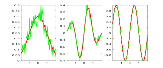
Figure 3: Small bandwidth effect, the ratio of two bad estimators is a good estimator. For bandwidth $h=0.01$ and $n=1000$, true (bold) and estimated $f$ (left), $b_{1}f$ (middle), and $b_{1}$ (right).

Table 4 presents the results for the estimation of $b$, either with the $CV_{{\rm NW}}$ criterion, with ratio of PCO of $bf$ and $f$, or with the ratio of the best estimators of $bf$ and $f$ in the collection. More precisely, the column ”Or” gives here the MISE computed with the estimator of $b$ obtained as a quotient of the two oracles of $bf$ and $f$ in each example and for each sample path. Clearly, the performance of the Nadaraya-Watson cross-validation criterion is much better, within a multiplicative factor from 2 and up to 6. The variance of the quotient estimators (oracle and PCO) are large, which shows that the mean performance is probably deteriorated by a few very bad results. However, the result is puzzling: even the ratio of the two best estimators of the numerator and denominator does not reach the good performance of the single-bandwidth CV method. Table 5 shows in addition that the selected bandwidths are in mean very small. We can check that the ratio of this bad numerator divided by a bad denominator fits well to the $b$ quotient function: this is illustrated by Figure 3. It is likely that both imply a compensation resulting in a locally, and thus also globally, better estimate. We can notice that the selected bandwidth also decrease more slowly when $n$ increases (see Table 5) than for the estimator of $bf$ (see Table 3). Our explanation (see the heuristic Remark 5.1 below) is that the risk of the Nadaraya-Watson estimator behaves as $C(h^{2\alpha}+\sigma^{2}/(nh))$, for some $\alpha>0$ related to the regularity of $b$, like in the projection least-squares method (see e.g. Baraud [1]). In the small noise case, $\sigma^{2}$ makes the variance term negligible, so that the bandwidth selection method aims at having small bias term $h^{2\alpha}$. On the other hand, the risk decomposition of the estimator of $bf$ involves a variance term of order $\|K\|_{2}^{2}\mathbb{E}(Y_{1}^{2})/(nh)$, and in all our examples, empirical evaluations of $\mathbb{E}(Y^{2})$ is in the range $[0.34,0.70]$, making the ratio with $\sigma^{2}$ between 34 and 70. In other words, the variance term for this estimator is 34 to 70 times larger. This is why it is important to investigate large noise case and a less favorable signal to noise ratio.

5.2.2 Large noise case

When setting $\sigma=0.7$, the empirical order of ${\mathbb{E}}(Y^{2})$ for the four models is between 0.91 and 1.31, which divided by $\sigma^{2}$ gives now a value between 1.85 and 2.67. This is much smaller than previously. This corresponds to a more difficult estimation problem, as can be seen from Figure 2.

	$b_{1}$			$b_{2}$
$n$	CV	PCO	Or	CV	PCO	Or
$250$	7.81	9.02	6.54	8.32	8.61	5.18
	(5.32)	(5.86)	(5.13)	(6.02)	(6.67)	(4.87)
$500$	4.33	4.34	3.25	4.57	4.83	3.02
	(3.09)	(2.71)	(2.15)	(2.86)	(4.07)	(2.58)
$1000$	2.26	2.19	1.72	2.38	2.13	1.40
	(1.37)	(1.30)	(1.16)	(1.39)	(2.04)	(1.15)

	$b_{3}$			$b_{4}$
$n$	CV	PCO	Or	CV	PCO	Or
$250$	16.2	18.5	14.8	7.84	9.36	7.89
	(8.47)	(10.3)	(9.06)	(4.94)	(4.62)	(4.94)
$500$	8.54	9.28	7.58	4.41	5.01	4.23
	(3.58)	(5.26)	(4.41)	(2.83)	(2.31)	(2.27)
$1000$	4.54	4.62	3.87	2.40	2.85	2.35
	(1.81)	(2.35)	(2.18)	(1.28)	(1.42)	(1.20)

Table 6: 100*MISE (with 100*std in parenthesis below) for the estimation of $b_{i}$, $i=1,\dots,4$, 200 repetitions, $X\sim{\mathcal{N}}(0,1)$, $\sigma=0.7$. CV and PCO are the two competing methods. Column ”Or” gives the average of ISE for the ratio of the two best estimators of $bf$ and $f$ in the collection.

We now comment the results given in Table 6. The MISE are quite larger, but in Figure 4, we show examples of estimated curves in this case, and the associated orders of MISEs, computed for 25 repetitions; they are not as good as for small noise, but still reasonable. The results in Table 6 show that the MISE have now the same orders, and the oracles can be much better than the results of the Nadarya-Watson estimator. The selected bandwidths are larger and decreasing with $n$ (see Table 7 in Appendix).

The conclusion of this study is that adaptive estimation of functions with kernel estimators and bandwidth selection relying on the PCO method proposed by Lacour et al. [13] gives very good results in theory and practice, not only for density estimation. However, for regression function estimation, one bandwidth selected with a criterion directly suited to the regression function is safer than the two different bandwidths selected when considering the Nadaraya-Watson estimator as a quotient of two functions that may be estimated separately. The results are not bad, but the strategy must be devoted to more complicated contexts where direct estimators of $b$ are not feasible.

Remark 5.1.

Note that if $h=h^{\prime}$, which means that $\widehat{b}_{n,h,h^{\prime}}$ is the usual Nadaraya-Watson estimator $\widehat{b}_{n,h}$,

$$\widehat{b}_{n,h}(x)=\sum_{i=1}^{n}w_{n,h}^{(i)}(x)\varepsilon_{i}\quad{\rm with}\quad w_{n,h}^{(i)}(x):=\frac{K((X_{i}-x)/h)}{\sum_{j=1}^{n}K((X_{j}-x)/h)}.$$

Then,

$$\widehat{b}_{n,h}(x)-b(x)=\sum_{i=1}^{n}w_{n,h}^{(i)}(x)(b(X_{i})-b(x))+\sum_{i=1}^{n}w_{n,h}^{(i)}(x)\varepsilon_{i},$$

and for a nonnegative kernel with compact support $[-1,1]$, if the regression function $b$ is Lispchitz continuous, then

$$\mathbb{E}[(\widehat{b}_{n,h}(x)-b(x))^{2}]\leqslant Ch^{2}+\sigma^{2}\mathbb{E}\left(\sum_{i=1}^{n}w_{n,h}^{(i)}(x)^{2}\right).$$

Moreover,

$$\mathbb{E}\left(\sum_{i=1}^{n}w_{n,h}^{(i)}(x)^{2}\right)=\frac{1}{nh}\mathbb{E}\left(\frac{\frac{1}{nh}\sum_{i=1}^{n}K((X_{i}-x)/h)^{2}}{[\frac{1}{nh}\sum_{i=1}^{n}K((X_{i}-x)/h)]^{2}}\right),$$

and for a fixed $h>0$, by the law of large numbers,

$$\frac{1}{nh}\sum_{i=1}^{n}K\left(\frac{X_{i}-x}{h}\right)^{2}\xrightarrow[n\rightarrow\infty]{{\rm a.s.}}\frac{1}{h}\mathbb{E}\left[K\left(\frac{X_{1}-x}{h}\right)^{2}\right]=\int_{-\infty}^{\infty}K(u)^{2}f(x+uh)du$$

and

$$\left[\frac{1}{nh}\sum_{i=1}^{n}K\left(\frac{X_{i}-x}{h}\right)\right]^{2} \xrightarrow[n\rightarrow\infty]{{\rm a.s.}} \mathbb{E}\left[\frac{1}{h}K\left(\frac{X_{1}-x}{h}\right)\right]^{2}$$

$$\hskip 56.9055pt=\left[\int_{-\infty}^{\infty}K(u)f(x+uh)du\right]^{2}.$$

Then, for small $h$, the first limit has order $\|K\|_{2}^{2}f(x)$ and the second one has order $f^{2}(x)$. To sum up, the risk of $\widehat{b}_{n,h}(x)$ is heuristically of order $Ch^{2}+\sigma^{2}\|K\|_{2}^{2}f(x)/(nh)$. This explains why, for small $\sigma^{2}$, the variance term gets small and the estimator can choose small bandwidth to make the bias as small as possible.

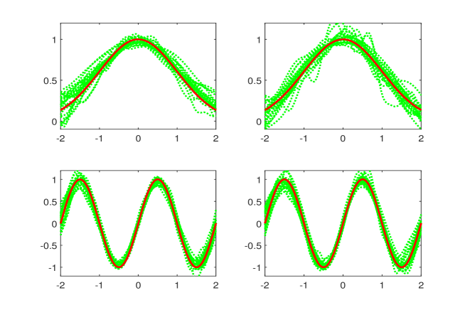
Figure 4: Example of 25 estimated $b$ with large noise $\sigma=0.7$, $n=1000$, true $b$ in bold red, estimated $b$ with sign-bandwidth CV selection (dotted green, left) and with ratio of PCO (dotted green, right) for functions 1 and 3. 100*MSE${}_{(100\;std)}$ are $2.62_{(1.64)}$ and $2.87_{(2.41)}$ (top) ; $4.71_{(1.74)}$ and $5.49_{(2.85)}$.

6 Proofs

6.1 Proof of Proposition 2.4

On the one hand, by Comte [4], Proposition 3.3.1,

$$\mathbb{E}(\|\widehat{f}_{n,h^{\prime}}-f\|_{2}^{2})\leqslant\|f-f_{h^{\prime}}\|_{2}^{2}+\frac{\mathfrak{c}_{K}}{nh^{\prime}}$$ (4)

and, by Proposition 2.2,

$$\mathbb{E}(\|\widehat{bf}_{n,h}-bf\|_{2}^{2})\leqslant\|bf-(bf)_{h}\|_{2}^{2}+\frac{\mathfrak{c}_{K,Y}}{nh}$$ (5)

For the proof of Inequality (4), the reader can also refer to Tsybakov [19]. On the other hand,

$$\widehat{b}_{n,h,h^{\prime}}-b=\left(\frac{\widehat{bf}_{n,h}-bf}{\widehat{f}_{n,h^{\prime}}}+bf\left(\frac{1}{\widehat{f}_{n,h^{\prime}}}-\frac{1}{f}\right)\right)\mathbf{1}_{\widehat{f}_{n,h^{\prime}}(.)>m_{n}/2}-b\mathbf{1}_{\widehat{f}_{n,h^{\prime}}(.)\leqslant m_{n}/2}.$$

Then,

$$\|\widehat{b}_{n,h,h^{\prime}}-b\|_{2,f,\mathcal{S}_{n}}^{2}$$

$$\hskip 28.45274pt\leqslant\frac{8\mathfrak{c}_{1}}{m_{n}^{2}}\left(\|\widehat{bf}_{n,h}-bf\|_{2}^{2}+\int_{-\infty}^{\infty}b(x)^{2}f(x)|\widehat{f}_{n,h^{\prime}}(x)-f(x)|^{2}dx\right)$$

$$\hskip 56.9055pt+2\int_{\mathcal{S}_{n}}b(x)^{2}f(x)\mathbf{1}_{|\widehat{f}_{n,h^{\prime}}(x)-f(x)|>m_{n}/2}dx$$

with $\mathfrak{c}_{1}:=\|f\|_{\infty}\vee\|f\|_{\infty}^{2}$.

By Markov’s inequality,

$$\mathbb{E}(\|\widehat{b}_{n,h,h^{\prime}}-b\|_{2,f,\mathcal{S}_{n}}^{2}) \leqslant \frac{8\mathfrak{c}_{1}}{m_{n}^{2}}(\mathbb{E}(\|\widehat{bf}_{n,h}-bf\|_{2}^{2})+\mathfrak{c}_{b,f}\mathbb{E}(\|\widehat{f}_{n,h^{\prime}}-f\|_{2}^{2}))$$

$$+2\mathfrak{c}_{b,f}\int_{\mathcal{S}_{n}}\mathbb{P}\left(|\widehat{f}_{n,h^{\prime}}(x)-f(x)|>\frac{m_{n}}{2}\right)dx$$

$$\leqslant \frac{8(\mathfrak{c}_{1}\vee 1)}{m_{n}^{2}}(\mathbb{E}(\|\widehat{bf}_{n,h}-bf\|_{2}^{2})+2\mathfrak{c}_{b,f}\mathbb{E}(\|\widehat{f}_{n,h^{\prime}}-f\|_{2}^{2})).$$

Inequalities (4) and (5) allow to conclude.

6.2 Proof of Theorem 3.2

First, let us prove the following lemma.

Lemma 6.1.

Consider

$$(bf)_{h}:=K_{h}\ast(bf)\quad\textrm{and}\quad(bf)_{h,\eta}:=K_{\eta}\ast K_{h}\ast(bf).$$

Then,

$$\mathbb{E}(\widehat{bf}_{n,h}(x))=(bf)_{h}(x)\quad\textrm{and}\quad\mathbb{E}(\widehat{bf}_{n,h,\eta}(x))=(bf)_{h,\eta}(x).$$

Proof.

Since $\mathbb{E}(\varepsilon_{k})=0$ and $X_{k}$ and $\varepsilon_{k}$ are independent for every $k\in\{1,\dots,n\}$,

$$\mathbb{E}(\widehat{bf}_{n,h}(x)) = \frac{1}{n}\sum_{k=1}^{n}\mathbb{E}(b(X_{k})K_{h}(X_{k}-x))+\frac{1}{n}\sum_{k=1}^{n}\mathbb{E}(\varepsilon_{k})\mathbb{E}(K_{h}(X_{k}-x))$$

$$= \int_{-\infty}^{\infty}K_{h}(y-x)b(y)f(y)dy=(bf)_{h}(x)$$

and

$$\mathbb{E}(\widehat{bf}_{n,h,\eta}(x)) = \frac{1}{n}\sum_{k=1}^{n}\mathbb{E}(b(X_{k})(K_{\eta}\ast K_{h})(X_{k}-x))$$

$$+\frac{1}{n}\sum_{k=1}^{n}\mathbb{E}(\varepsilon_{k})\mathbb{E}((K_{\eta}\ast K_{h})(X_{k}-x))$$

$$= \int_{-\infty}^{\infty}(K_{\eta}\ast K_{h})(y-x)b(y)f(y)dy=(bf)_{h,\eta}(x).$$

∎

Since

$$\widehat{h}_{n}\in\arg\min_{h\in\mathcal{H}_{n}}\{A_{n}(h)+V_{n}(h)\},$$

for every $h\in\mathcal{H}_{n}$,

$$\mathbb{E}(\|\widehat{bf}_{n,\widehat{h}_{n}}-bf\|_{2}^{2})\leqslant 3\mathbb{E}(\|\widehat{bf}_{n,h}-bf\|_{2}^{2})+6V_{n}(h)+6\mathbb{E}(A_{n}(h))$$ (6)

Let us find a suitable control of $\mathbb{E}(A_{n}(h))$. First of all, for any $h,\eta\in\mathcal{H}_{n}$,

$$\|\widehat{bf}_{n,h,\eta}-\widehat{bf}_{n,\eta}\|_{2}^{2} \leqslant 3(\|\widehat{bf}_{n,h,\eta}-(bf)_{h,\eta}\|_{2}^{2}$$

$$+\|\widehat{bf}_{n,\eta}-(bf)_{\eta}\|_{2}^{2}+\|(bf)_{h,\eta}-(bf)_{\eta}\|_{2}^{2}).$$

Then,

$$A_{n}(h) \leqslant 3\left[\sup_{\eta\in\mathcal{H}_{n}}\left(\|\widehat{bf}_{n,h,\eta}-(bf)_{h,\eta}\|_{2}^{2}-\frac{V_{n}(\eta)}{6}\right)_{+}\right.$$

$$\left.+\sup_{\eta\in\mathcal{H}_{n}}\left(\|\widehat{bf}_{n,\eta}-(bf)_{\eta}\|_{2}^{2}-\frac{V_{n}(\eta)}{6}\right)_{+}+\|(bf)_{h,\eta}-(bf)_{\eta}\|_{2}^{2}\right].$$

On the one hand,

$$\|(bf)_{h,\eta}-(bf)_{\eta}\|_{2}=\|K_{\eta}\ast(K_{h}\ast(bf)-bf)\|_{2}\leqslant\|K\|_{1}\|bf-(bf)_{h}\|_{2}.$$

On the other hand, let $\mathcal{C}$ be a countable and dense subset of the unit sphere of $\mathbb{L}^{2}(\mathbb{R},dx)$ and consider $\mathfrak{m}(n)>0$. Then, by Lemma 6.1,

$$\mathbb{E}\left[\sup_{\eta\in\mathcal{H}_{n}}\left(\|\widehat{bf}_{n,\eta}-(bf)_{\eta}\|_{2}^{2}-\frac{V_{n}(\eta)}{6}\right)_{+}\right]$$

$$\hskip 56.9055pt\leqslant\sum_{\eta\in\mathcal{H}_{n}}\mathbb{E}\left(\left(\sup_{\psi\in\mathcal{C}}2\mathbf{V}_{n,\eta}(\psi)^{2}-\frac{V_{n}(\eta)}{6}\right)_{+}\right)+2\sum_{\eta\in\mathcal{H}_{n}}\mathbb{E}(\mathbf{W}_{n,\eta})$$

where, for any $\psi\in\mathcal{C}$,

$$\mathbf{V}_{n,\eta}(\psi):=\frac{1}{n}\sum_{k=1}^{n}(v_{\psi,n,\eta}(X_{k},Y_{k})-\mathbb{E}(v_{\psi,n,\eta}(X_{k},Y_{k})))$$

with

$$v_{\psi,n,\eta}(x,y):=y\mathbf{1}_{|y|\leqslant\mathfrak{m}(n)}\int_{-\infty}^{\infty}\psi(u)K_{\eta}(x-u)du\textrm{ $;$ }\forall(x,y)\in\mathbb{R}^{2},$$

and

$$\mathbf{W}_{n,\eta}:=\frac{1}{n}\sum_{k=1}^{n}\int_{-\infty}^{\infty}|Y_{k}\mathbf{1}_{|Y_{k}|>\mathfrak{m}(n)}K_{\eta}(X_{k}-u)-\mathbb{E}(Y_{k}\mathbf{1}_{|Y_{k}|>\mathfrak{m}(n)}K_{\eta}(X_{k}-u))|^{2}du.$$

In order to apply Talagrand’s inequality (see Klein and Rio [12]), we compute bounds.

• For every $\psi\in\mathcal{C}$, $x\in\mathbb{R}$ and $y\in[-\mathfrak{m}(n),\mathfrak{m}(n)]$,

  $$|v_{\psi,n,\eta}(x,y)| \leqslant |y|\int_{-\infty}^{\infty}|\psi(u)|\cdot|K_{\eta}(u-x)|du$$

  $$\leqslant |y|\cdot\|K_{\eta}(\cdot-x)\|_{2}\leqslant\frac{\mathfrak{m}(n)\|K\|_{2}}{\sqrt{\eta}}.$$

  Then,

  $$\sup_{\psi\in\mathcal{C}}\|v_{\psi,n,\eta}\|_{\infty}\leqslant\mathfrak{m}_{1}(n,\eta):=\frac{\mathfrak{m}(n)\|K\|_{2}}{\sqrt{\eta}}.$$

• By Proposition 2.4 and Lemma 6.1,

  $$\mathbb{E}\left(\sup_{\psi\in\mathcal{C}}\mathbf{V}_{n,\eta}(\psi)^{2}\right) \leqslant \int_{-\infty}^{\infty}\textrm{var}(\widehat{bf}_{n,\eta}(u))du$$

  $$\leqslant \mathfrak{m}_{2}(n,\eta):=\frac{\mathfrak{c}_{K,Y}}{n\eta}.$$

• For any $\psi\in\mathcal{C}$ and $k\in\{1,\dots,n\}$,

  $$\textrm{var}(v_{\psi,n,\eta}(X_{k},Y_{k}))$$

  $$\hskip 28.45274pt\leqslant\mathbb{E}\left(\left|Y_{k}\int_{-\infty}^{\infty}\psi(u)K_{\eta}(X_{k}-u)du\right|^{2}\right)$$

  $$\hskip 28.45274pt\leqslant\mathbb{E}((K_{\eta}\ast\psi)(X_{1})^{4})^{1/2}\mathbb{E}(Y_{1}^{4})^{1/2}\leqslant\|f\|_{\infty}^{1/2}\|K_{\eta}\ast\psi\|_{4}^{2}\mathbb{E}(Y_{1}^{4})^{1/2}.$$

  By Young’s inequality, $\|K_{\eta}\ast\psi\|_{4}\leqslant\|\psi\|_{2}\|K_{\eta}\|_{4/3}$. So,

  $$\textrm{var}(v_{\psi,n,\eta}(X_{k},Y_{k}))\leqslant\mathfrak{m}_{3}:=\frac{\mathfrak{m}_{f,K}}{\sqrt{\eta}}$$

  with $\mathfrak{m}_{f,K}:=\|f\|_{\infty}^{1/2}\|K\|_{4/3}^{2}\mathbb{E}(Y_{1}^{4})^{1/2}$.

By applying Talagrand’s inequality to $(v_{\psi,n,\eta})_{\psi\in\mathcal{C}}$ and to the independent random variables $(X_{1},Y_{1}),\dots,(X_{n},Y_{n})$, there exist three constants $\mathfrak{c}_{1},\mathfrak{c}_{2},\mathfrak{c}_{3}>0$, not depending on $n$ and $\eta$, such that

$$\mathbb{E}\left(\left(\sup_{\psi\in\mathcal{C}}\mathbf{V}_{n,\eta}(\psi)^{2}-4\mathfrak{m}_{2}(n,\eta)\right)_{+}\right)$$

$$\hskip 21.33955pt\leqslant\mathfrak{c}_{1}\left(\frac{\mathfrak{m}_{3}}{n}\exp\left(-\mathfrak{c}_{2}\frac{n\mathfrak{m}_{2}(n,\eta)}{\mathfrak{m}_{3}}\right)+\frac{\mathfrak{m}_{1}(n,\eta)^{2}}{n^{2}}\exp\left(-\mathfrak{c}_{3}\frac{n\mathfrak{m}_{2}(n,\eta)^{1/2}}{\mathfrak{m}_{1}(n,\eta)}\right)\right)$$

$$\hskip 21.33955pt=\mathfrak{c}_{1}\left[\frac{\mathfrak{m}_{f,K}}{n\sqrt{\eta}}\exp\left(-\frac{\mathfrak{c}_{2}\mathfrak{c}_{K,Y}}{\mathfrak{m}_{f,K}\sqrt{\eta}}\right)+\frac{1}{n^{2}\eta}\mathfrak{m}(n)^{2}\|K\|_{2}^{2}\exp\left(-\sqrt{n}\frac{\mathfrak{c}_{3}\mathbb{E}(Y_{1}^{2})^{1/2}}{\mathfrak{m}(n)}\right)\right].$$

By taking $\mathfrak{m}(n):=\mathfrak{c}_{3}\mathbb{E}(Y_{1}^{2})^{1/2}n^{1/2}/\log(n)^{1/2}$,

$$\mathbb{E}\left(\left(\sup_{\psi\in\mathcal{C}}\mathbf{V}_{n,\eta}(\psi)^{2}-4\mathfrak{m}_{2}(n,\eta)\right)_{+}\right)$$

$$\hskip 56.9055pt\leqslant\frac{\mathfrak{c}_{1}}{n}\left[\frac{\mathfrak{m}_{f,K}}{\sqrt{\eta}}\exp\left(-\frac{\mathfrak{c}_{2}\mathfrak{c}_{K,Y}}{\mathfrak{m}_{f,K}\sqrt{\eta}}\right)\right.\left.+\frac{\mathfrak{c}_{3}^{2}\mathbb{E}(Y_{1}^{2})\|K\|_{2}^{2}}{\eta n\log(n)}\right].$$

By the conditional Markov inequality,

$$\mathbb{E}(\mathbf{W}_{n,\eta}) \leqslant \int_{-\infty}^{\infty}\mathbb{E}(Y_{1}^{2}\mathbf{1}_{|Y_{1}|>\mathfrak{m}(n)}K_{\eta}(X_{1}-z)^{2})dz$$

$$= \frac{\|K\|_{2}^{2}}{\eta}\cdot\mathbb{E}(Y_{1}^{2}\mathbb{E}(\mathbf{1}_{|Y_{1}|>\mathfrak{m}(n)}|Y_{1}))$$

$$\leqslant \frac{\|K\|_{2}^{2}}{\eta\mathfrak{m}(n)^{4}}\mathbb{E}(Y_{1}^{6})=\mathfrak{c}_{3}^{-4}\mathbb{E}(Y_{1}^{2})^{-2}\mathbb{E}(Y_{1}^{6})\|K\|_{2}^{2}\frac{\log(n)^{2}}{n^{2}\eta}.$$

Finally, for $\upsilon\geqslant 48$,

$$\frac{V_{n}(\eta)}{12}\geqslant 4\mathfrak{m}_{2}(n,\eta).$$

Then, since

$$\frac{1}{n}\sum_{\eta\in\mathcal{H}_{n}}\frac{1}{\eta}\leqslant\mathfrak{m},\quad\textrm{and}\quad\sum_{\eta\in\mathcal{H}_{n}}\frac{1}{\sqrt{\eta}}\exp\left(-\frac{c}{\sqrt{\eta}}\right)\leqslant\mathfrak{m}(c)\textrm{ $;$ }\forall c>0,$$

there exists a constant $\mathfrak{c}_{4}>0$, not depending on $n$, such that

$$\mathbb{E}\left[\sup_{\eta\in\mathcal{H}_{n}}\left(\|\widehat{bf}_{n,\eta}-(bf)_{\eta}\|_{2}^{2}-\frac{V_{n}(\eta)}{6}\right)_{+}\right]$$

$$\hskip 28.45274pt\leqslant 2\sum_{\eta\in\mathcal{H}_{n}}\mathbb{E}\left[\left(\sup_{\psi\in\mathcal{C}}\mathbf{V}_{n,\eta}(\psi)^{2}-4\mathfrak{m}_{2}(n,\eta)\right)_{+}\right]+2\sum_{\eta\in\mathcal{H}_{n}}\mathbb{E}(\mathbf{W}_{n,\eta})$$

$$\hskip 28.45274pt\leqslant\mathfrak{c}_{4}\frac{\log(n)^{2}}{n}$$ (8)

The same ideas give that there exists a constant $\mathfrak{c}_{5}>0$, not depending on $n$ and $h$, such that

$$\mathbb{E}\left[\sup_{\eta\in\mathcal{H}_{n}}\left(\|\widehat{bf}_{n,h,\eta}-(bf)_{h,\eta}\|_{2}^{2}-\frac{V_{n}(\eta)}{6}\right)_{+}\right]\leqslant\mathfrak{c}_{5}\frac{\log(n)^{2}}{n}$$ (9)

Therefore, by Inequalities (6)–(9), there exist two deterministic constants $\mathfrak{c},\overline{\mathfrak{c}}>0$, not depending on $n$, such that

$$\mathbb{E}(\|\widehat{bf}_{n,\widehat{h}_{n}}-bf\|_{2}^{2})\leqslant\mathfrak{c}\cdot\inf_{h\in\mathcal{H}_{n}}\{\|(bf)_{h}-bf\|_{2}^{2}+V_{n}(h)\}+\overline{\mathfrak{c}}\frac{\log(n)^{2}}{n}.$$

6.3 Proof of Corollary 3.3

As established in the proof of Proposition 2.4,

$$\|\widehat{b}_{n,\widehat{h}_{n},\widehat{h}_{n}^{\prime}}-b\|_{2,f,\mathcal{S}_{n}}^{2}$$

$$\hskip 28.45274pt\leqslant\frac{8\mathfrak{c}_{1}}{m_{n}^{2}}\left(\|\widehat{bf}_{n,\widehat{h}_{n}}-bf\|_{2}^{2}+\mathfrak{c}_{b,f}\int_{-\infty}^{\infty}|\widehat{f}_{n,\widehat{h}_{n}^{\prime}}(x)-f(x)|^{2}dx\right)$$

$$\hskip 56.9055pt+2\mathfrak{c}_{b,f}\int_{\mathcal{S}_{n}}\mathbf{1}_{|\widehat{f}_{n,\widehat{h}_{n}^{\prime}}(x)-f(x)|>m_{n}/2}dx$$

with $\mathfrak{c}_{1}:=\|f\|_{\infty}\vee\|f\|_{\infty}^{2}$. By Markov’s inequality,

$$\mathbb{E}(\|\widehat{b}_{n,\widehat{h}_{n},\widehat{h}_{n}^{\prime}}-b\|_{2,f,\mathcal{S}_{n}}^{2}) \leqslant \frac{8\mathfrak{c}_{1}}{m_{n}^{2}}(\mathbb{E}(\|\widehat{bf}_{n,\widehat{h}_{n}}-bf\|_{2}^{2})+\mathfrak{c}_{b,f}\mathbb{E}(\|\widehat{f}_{n,\widehat{h}_{n}^{\prime}}-f\|_{2}^{2}))$$

$$+2\mathfrak{c}_{b,f}\int_{\mathcal{S}_{n}}\mathbb{P}\left(|\widehat{f}_{n,\widehat{h}_{n}^{\prime}}(x)-f(x)|>\frac{m_{n}}{2}\right)dx$$

$$\leqslant \frac{8(\mathfrak{c}_{1}\vee 1)}{m_{n}^{2}}(\mathbb{E}(\|\widehat{bf}_{n,\widehat{h}_{n}}-bf\|_{2}^{2})$$

$$\hskip 85.35826pt+2\mathfrak{c}_{b,f}\mathbb{E}(\|\widehat{f}_{n,\widehat{h}_{n}^{\prime}}-f\|_{2}^{2})).$$

Theorem 3.2 and Inequality (2) allow to conclude.

6.4 Proof of Theorem 4.2

The proof relies on three lemmas, which are stated first.

Lemma 6.2.

Consider the $U$-statistic

$$U_{n}(h,h_{\min}):=\sum_{k\not=l}\langle Y_{k}K_{h}(X_{k}-\cdot)-(bf)_{h},Y_{l}K_{h_{\min}}(X_{l}-\cdot)-(bf)_{h_{\min}}\rangle_{2}.$$

Under Assumption 2.1, if there exists $\alpha>0$ such that $\mathbb{E}(\exp(\alpha|Y_{1}|))<\infty$, then there exists a deterministic constant $\mathfrak{c}_{U}>0$, not depending on $n$ and $h_{\min}$, such that for every $\vartheta\in(0,1)$,

$$\mathbb{E}\left(\sup_{h\in\mathcal{H}_{n}}\left\{\frac{|U_{n}(h,h_{\min})|}{n^{2}}-\frac{\vartheta\|K\|_{2}^{2}}{nh}\mathbb{E}(Y_{1}^{2})\right\}\right)\leqslant\mathfrak{c}_{U}\frac{\log(n)^{5}}{\vartheta n}.$$

Lemma 6.3.

For every $\eta,\eta^{\prime}\in\mathcal{H}_{n}$, consider

$$V_{n}(\eta,\eta^{\prime}):=\langle\widehat{bf}_{n,\eta}-(bf)_{\eta^{\prime}},(bf)_{\eta^{\prime}}-bf\rangle_{2}.$$

Under Assumption 2.1, if there exists $\alpha>0$ such that $\mathbb{E}(\exp(\alpha|Y_{1}|))<\infty$ and $bf$ is bounded, then there exists a deterministic constant $\mathfrak{c}_{V}>0$, not depending on $n$ and $h_{\min}$, such that for every $\vartheta\in(0,1)$,

$$\mathbb{E}\left(\sup_{\eta,\eta^{\prime}\in\mathcal{H}_{n}}\{|V_{n}(\eta,\eta^{\prime})|-\vartheta\|(bf)_{\eta^{\prime}}-bf\|_{2}^{2}\}\right)\leqslant\mathfrak{c}_{V}\frac{\log(n)^{3}}{\vartheta n}.$$

Lemma 6.4.

Under Assumption 2.1, if $bf$ is bounded and if there exists $\alpha>0$ such that $\mathbb{E}(\exp(\alpha|Y_{1}|))<\infty$, then there exists a deterministic constant $\mathfrak{c}_{L}>0$, not depending on $n$ and $h_{\min}$, such that for every $\vartheta\in(0,1)$,

$$\mathbb{E}\left(\sup_{h\in\mathcal{H}_{n}}\left\{\|(bf)_{h}-bf\|_{2}^{2}+\frac{\mathfrak{c}_{K,Y}}{nh}-\frac{1}{1-\vartheta}\|\widehat{bf}_{n,h}-bf\|_{2}^{2}\right\}\right)\leqslant\frac{\mathfrak{c}_{L}}{\vartheta(1-\vartheta)}\cdot\frac{\log(n)^{5}}{n}.$$

6.4.1 Steps of the proof.

The proof of Theorem 4.2 is dissected in three steps.

Step 1. In this step, a suitable decomposition of

$$\|\widehat{bf}_{n,\widetilde{h}_{n}}-bf\|_{2}^{2}$$

is provided. On the one hand,

$$\|\widehat{bf}_{n,\widetilde{h}_{n}}-bf\|_{2}^{2}+\textrm{pen}(\widetilde{h}_{n})$$

$$\hskip 28.45274pt=\|\widehat{bf}_{n,\widetilde{h}_{n}}-\widehat{bf}_{n,h_{\min}}\|_{2}^{2}+\textrm{pen}(\widetilde{h}_{n})$$

$$\hskip 56.9055pt+\|\widehat{bf}_{n,h_{\min}}-bf\|_{2}^{2}-2\langle\widehat{bf}_{n,h_{\min}}-\widehat{bf}_{n,\widetilde{h}_{n}},\widehat{bf}_{n,h_{\min}}-bf\rangle_{2}.$$

Since

$$\widetilde{h}_{n}\in\arg\min_{h\in\mathcal{H}_{n}}\textrm{crit}(h)\quad{\rm with}\quad\textrm{crit}(h)=\|\widehat{bf}_{n,h}-\widehat{bf}_{n,h_{\min}}\|_{2}^{2}+\textrm{pen}(h),$$

for any $h\in\mathcal{H}_{n}$,

$$\|\widehat{bf}_{n,\widetilde{h}_{n}}-bf\|_{2}^{2}\leqslant\|\widehat{bf}_{n,h}-bf\|_{2}^{2}+\textrm{pen}(h)-2\psi_{n}(h)-(\textrm{pen}(\widetilde{h}_{n})-2\psi_{n}(\widetilde{h}_{n}))$$ (10)

with

$$\psi_{n}(h):=\langle\widehat{bf}_{n,h_{\min}}-bf,\widehat{bf}_{n,h}-bf\rangle_{2}.$$

On the other hand,

$$\psi_{n}(h)=\psi_{1,n}(h)+\psi_{2,n}(h)+\psi_{3,n}(h)$$

where

$$\psi_{1,n}(h) := \frac{\langle K_{h_{\min}},K_{h}\rangle_{2}}{n^{2}}\sum_{k=1}^{n}Y_{k}^{2}+\frac{U_{n}(h,h_{\min})}{n^{2}},$$

$$\psi_{2,n}(h) := -\frac{1}{n^{2}}\left(\sum_{k=1}^{n}Y_{k}\langle K_{h_{\min}}(X_{k}-\cdot),(bf)_{h}\rangle_{2}\right.$$

$$\left.+\sum_{k=1}^{n}Y_{k}\langle K_{h}(X_{k}-\cdot),(bf)_{h_{\min}}\rangle_{2}\right)+\frac{1}{n}\langle(bf)_{h_{\min}},(bf)_{h}\rangle_{2}\textrm{ and}$$

$$\psi_{3,n}(h) := V_{n}(h,h_{\min})+V_{n}(h_{\min},h)+\langle(bf)_{h}-bf,(bf)_{h_{\min}}-bf\rangle_{2}.$$

Step 2. In this step, let us provide some suitable controls of

$$\mathbb{E}(\psi_{i,n}(h))\textrm{ and }\mathbb{E}(\psi_{i,n}(\widetilde{h}_{n}))\textrm{ $;$ }i=1,2,3.$$

1. Consider

   $$\widetilde{\psi}_{1,n}(h):=\psi_{1,n}(h)-\frac{\langle K_{h_{\min}},K_{h}\rangle_{2}}{n^{2}}\sum_{k=1}^{n}Y_{k}^{2}=\frac{U(h,h_{\min})}{n^{2}}.$$

   By Lemma 6.2,

   $$\mathbb{E}(|\widetilde{\psi}_{1,n}(h)|)\leqslant\frac{\theta\|K\|_{2}^{2}}{nh}\mathbb{E}(Y_{1}^{2})+\frac{2\mathfrak{c}_{U}}{\theta}\cdot\frac{\log(n)^{5}}{n}$$

   and

   $$\mathbb{E}(|\widetilde{\psi}_{1,n}(\widetilde{h}_{n})|)\leqslant\mathbb{E}\left(\frac{\theta\|K\|_{2}^{2}}{n\widetilde{h}_{n}}\right)\mathbb{E}(Y_{1}^{2})+\frac{2\mathfrak{c}_{U}}{\theta}\cdot\frac{\log(n)^{5}}{n}.$$

2. On the one hand, for every $\eta,\eta^{\prime}\in\mathcal{H}_{n}$, consider

   $$\Psi_{2,n}(\eta,\eta^{\prime}):=\frac{1}{n}\sum_{k=1}^{n}Y_{k}\langle K_{\eta}(X_{k}-\cdot),(bf)_{\eta^{\prime}}\rangle_{2}.$$

   Then,

   $$\mathbb{E}\left(\sup_{\eta,\eta^{\prime}\in\mathcal{H}_{n}}|\Psi_{2,n}(\eta,\eta^{\prime})|\right)$$

   $$\hskip 28.45274pt\leqslant\mathbb{E}\left(|Y_{1}|\sup_{\eta,\eta^{\prime}\in\mathcal{H}_{n}}\int_{-\infty}^{\infty}|K_{\eta}(X_{1}-u)(bf)_{\eta^{\prime}}(u)|du\right)$$

   $$\hskip 28.45274pt\leqslant\mathbb{E}(Y_{1}^{2})^{1/2}\|K\|_{1}^{2}\|bf\|_{\infty}.$$

   On the other hand,

   $$\sup_{\eta,\eta^{\prime}\in\mathcal{H}_{n}}|\langle(bf)_{\eta},(bf)_{\eta^{\prime}}\rangle_{2}| \leqslant \sup_{\eta,\eta^{\prime}\in\mathcal{H}_{n}}\|K_{\eta}\ast(bf)\|_{2}\|K_{\eta^{\prime}}\ast(bf)\|_{2}$$

   $$\leqslant \|K\|_{1}^{2}\|bf\|_{2}^{2}\leqslant\mathbb{E}(Y_{1}^{2})^{1/2}\|K\|_{1}^{2}\|bf\|_{\infty}.$$

   Then,

   $$\mathbb{E}(|\psi_{2,n}(h)|)\leqslant\frac{3}{n}\mathbb{E}(Y_{1}^{2})^{1/2}\|K\|_{1}^{2}\|bf\|_{\infty}$$

   and

   $$\mathbb{E}(|\psi_{2,n}(\widetilde{h}_{n})|)\leqslant\frac{3}{n}\mathbb{E}(Y_{1}^{2})^{1/2}\|K\|_{1}^{2}\|bf\|_{\infty}.$$

3. By Lemma 6.3,

   $$\mathbb{E}(|\psi_{n,3}(h)|) \leqslant \frac{\theta}{2}(\|(bf)_{h}-bf\|_{2}^{2}+\|(bf)_{h_{\min}}-bf\|_{2}^{2})+4\mathfrak{c}_{V}\frac{\log(n)^{3}}{\theta n}$$

   $$+\left(\frac{\theta}{2}\right)^{1/2}\|(bf)_{h}-bf\|_{2}\times\left(\frac{2}{\theta}\right)^{1/2}\|(bf)_{h_{\min}}-bf\|_{2}$$

   $$\leqslant \theta\|(bf)_{h}-bf\|_{2}^{2}+\left(\frac{\theta}{2}+\frac{2}{\theta}\right)\|(bf)_{h_{\min}}-bf\|_{2}^{2}$$

   $$+4\mathfrak{c}_{V}\frac{\log(n)^{3}}{\theta n}$$

   and

   $$\mathbb{E}(|\psi_{n,3}(\widetilde{h}_{n})|) \leqslant \theta\mathbb{E}(\|(bf)_{\widetilde{h}_{n}}-bf\|_{2}^{2})$$

   $$+\left(\frac{\theta}{2}+\frac{2}{\theta}\right)\|(bf)_{h_{\min}}-bf\|_{2}^{2}+4\mathfrak{c}_{V}\frac{\log(n)^{3}}{\theta n}.$$

Step 3. Consider

$$\widetilde{\psi}_{n}(h):=\psi_{n}(h)-\frac{\langle K_{h_{\min}},K_{h}\rangle_{2}}{n^{2}}\sum_{k=1}^{n}Y_{k}^{2}.$$

By Step 2, there exists a deterministic constant $\mathfrak{c}_{U,V}>0$, not depending on $n$, $h$ and $h_{\min}$, such that

$$\mathbb{E}(|\widetilde{\psi}_{n}(h)|) \leqslant \theta\left(\|(bf)_{h}-bf\|_{2}^{2}+\frac{\mathfrak{c}_{K,Y}}{nh}\right)$$

$$+\frac{\mathfrak{c}_{U,V}}{\theta}\cdot\frac{\log(n)^{5}}{n}+\left(\frac{\theta}{2}+\frac{2}{\theta}\right)\|(bf)_{h_{\min}}-bf\|_{2}^{2}$$

and

$$\mathbb{E}(|\widetilde{\psi}_{n}(\widetilde{h}_{n})|) \leqslant \theta\left[\mathbb{E}(\|(bf)_{\widetilde{h}_{n}}-bf\|_{2}^{2})+\mathbb{E}\left(\frac{\mathfrak{c}_{K,Y}}{n\widetilde{h}_{n}}\right)\right]$$

$$+\frac{\mathfrak{c}_{U,V}}{\theta}\cdot\frac{\log(n)^{5}}{n}+\left(\frac{\theta}{2}+\frac{2}{\theta}\right)\|(bf)_{h_{\min}}-bf\|_{2}^{2}.$$

Then, by Lemma 6.4,

$$\mathbb{E}(|\widetilde{\psi}_{n}(h)|) \leqslant \frac{\theta}{1-\theta}\mathbb{E}(\|\widehat{bf}_{n,h}-bf\|_{2}^{2})+\left(\frac{\theta}{2}+\frac{2}{\theta}\right)\|(bf)_{h_{\min}}-bf\|_{2}^{2}$$

$$+\left(\frac{\mathfrak{c}_{U,V}}{\theta}+\frac{\mathfrak{c}_{L}}{1-\theta}\right)\frac{\log(n)^{5}}{n}$$

and

$$\mathbb{E}(|\widetilde{\psi}_{n}(\widetilde{h}_{n})|) \leqslant \frac{\theta}{1-\theta}\mathbb{E}(\|\widehat{bf}_{n,\widetilde{h}_{n}}-bf\|_{2}^{2})+\left(\frac{\theta}{2}+\frac{2}{\theta}\right)\|(bf)_{h_{\min}}-bf\|_{2}^{2}$$

$$+\left(\frac{\mathfrak{c}_{U,V}}{\theta}+\frac{\mathfrak{c}_{L}}{1-\theta}\right)\frac{\log(n)^{5}}{n}.$$

By Inequality (10), there exist two deterministic constant $\mathfrak{c}_{1},\mathfrak{c}_{2}>0$, not depending on $n$, $h$ and $h_{\min}$, such that

$$\mathbb{E}(\|\widehat{bf}_{n,\widetilde{h}_{n}}-bf\|_{2}^{2}) \leqslant \mathbb{E}(\|\widehat{bf}_{n,h}-bf\|_{2}^{2})+2(\mathbb{E}(|\widetilde{\psi}_{n}(h)|)+\mathbb{E}(|\widetilde{\psi}_{n}(\widetilde{h}_{n})|))$$

$$\leqslant \left(1+\frac{2\theta}{1-\theta}\right)\mathbb{E}(\|\widehat{bf}_{n,h}-bf\|_{2}^{2})$$

$$+\frac{2\theta}{1-\theta}\mathbb{E}(\|\widehat{bf}_{n,\widetilde{h}_{n}}-bf\|_{2}^{2})$$

$$+\frac{\mathfrak{c}_{1}}{\theta}\|(bf)_{h_{\min}}-bf\|_{2}^{2}+\frac{\mathfrak{c}_{2}}{\theta(1-\theta)}\cdot\frac{\log(n)^{5}}{n}.$$

This concludes the proof.

6.4.2 Proof of Lemma 6.2

Consider

$$\Delta_{n}:=\{(k,l)\in\{1,\dots,n\}:2\leqslant k\textrm{ and }l<k\}$$

and $Z_{k}:=(X_{k},Y_{k})$ for every $k\in\{1,\dots,n\}$.

On the one hand, consider $n\in\mathbb{N}$ such that $\mathfrak{m}(n):=4\log(n)/\alpha\geqslant 1$ and

$$U_{1,n}(h,h_{\min}):=\sum_{k=2}^{n}\sum_{l<k}(G_{n,h,h_{\min}}(Z_{k},Z_{l})+G_{n,h_{\min},h}(Z_{k},Z_{l}))$$

where, for every $\eta,\eta^{\prime}\in\{h,h_{\min}\}$ and $z,z^{\prime}\in\mathbb{R}^{2}$,

$$G_{n,\eta,\eta^{\prime}}(z,z^{\prime}):=$$

$$\hskip 21.33955pt\langle z_{2}\mathbf{1}_{|z_{2}|\leqslant\mathfrak{m}(n)}K_{\eta}(z_{1}-\cdot)-(bf)_{n,\eta},z_{2}^{\prime}\mathbf{1}_{|z_{2}^{\prime}|\leqslant\mathfrak{m}(n)}K_{\eta^{\prime}}(z_{1}^{\prime}-\cdot)-(bf)_{n,\eta^{\prime}}\rangle_{2}$$

and

$$(bf)_{n,\eta}:=\mathbb{E}(Y_{1}\mathbf{1}_{|Y_{1}|\leqslant\mathfrak{m}(n)}K_{\eta}(X_{1}-\cdot)).$$

For every $\eta,\eta^{\prime}\in\{h,h_{\min}\}$ and $(k,l)\in\Delta_{n}$,

$$\mathbb{E}(G_{n,\eta,\eta^{\prime}}(Z_{k},Z_{l})|Z_{k}) = \int_{-\infty}^{\infty}(Y_{k}\mathbf{1}_{|Y_{k}|\leqslant\mathfrak{m}(n)}K_{\eta}(X_{k}-z)-(bf)_{n,\eta}(z))$$

$$\times\mathbb{E}(Y_{l}\mathbf{1}_{|Y_{l}|\leqslant\mathfrak{m}(n)}K_{\eta^{\prime}}(X_{l}-z)-(bf)_{n,\eta^{\prime}}(z))dz=0.$$

So, by Houdré and Reynaud-Bouret [10], Theorem 3.4, there exists a universal constant $\mathfrak{e}>0$ such that

$$\mathbb{P}(|U_{1,n}(h,h_{\min})|\geqslant\mathfrak{e}(\mathfrak{c}_{n}\lambda^{1/2}+\mathfrak{d}_{n}\lambda+\mathfrak{b}_{n}\lambda^{3/2}+\mathfrak{a}_{n}\lambda^{2}))\leqslant 5.54e^{-\lambda}$$ (11)

where the constants $\mathfrak{a}_{n}$, $\mathfrak{b}_{n}$, $\mathfrak{c}_{n}$ and $\mathfrak{d}_{n}$ will be defined and controlled in the sequel.

• The constant $\mathfrak{a}_{n}$. Consider

  $$\mathfrak{a}_{n}:=\sup_{(z,z^{\prime})\in\mathbb{R}^{2}\times\mathbb{R}^{2}}\mathbf{A}_{n}(z,z^{\prime}),$$

  where

  $$\mathbf{A}_{n}(z,z^{\prime}):=|G_{n,h,h_{\min}}(z,z^{\prime})+G_{n,h_{\min},h}(z,z^{\prime})|\textrm{ $;$ }\forall z,z^{\prime}\in\mathbb{R}^{2}.$$

  First, note that for every $\eta\in\mathcal{H}_{n}$,

  $$\|(bf)_{n,\eta}\|_{1}\leqslant\mathbb{E}(|Y_{1}|\mathbf{1}_{|Y_{1}|\leqslant\mathfrak{m}(n)})\|K\|_{1}\leqslant\mathfrak{m}(n)\|K\|_{1}$$

  and

  $$\|(bf)_{n,\eta}\|_{\infty}\leqslant\frac{\mathfrak{m}(n)\|K\|_{\infty}}{\eta}.$$

  For any $z,z^{\prime}\in\mathbb{R}\times[-\mathfrak{m}(n),\mathfrak{m}(n)]$,

  $$\mathbf{A}_{n}(z,z^{\prime}) \leqslant \langle z_{2}K_{h}(z_{1}-\cdot)-(bf)_{n,h},z_{2}^{\prime}K_{h_{\min}}(z_{1}^{\prime}-\cdot)-(bf)_{n,h_{\min}}\rangle_{2}$$

  $$+\langle z_{2}K_{h_{\min}}(z_{1}-\cdot)-(bf)_{n,h_{\min}},z_{2}^{\prime}K_{h}(z_{1}^{\prime}-\cdot)-(bf)_{n,h}\rangle_{2}$$

  $$\leqslant 2(\mathfrak{m}(n)\|K_{h_{\min}}\|_{\infty}+\|(bf)_{n,h_{\min}}\|_{\infty})$$

  $$\times(\mathfrak{m}(n)\|K\|_{1}+\|(bf)_{n,h}\|_{1})$$

  $$\leqslant \frac{8\|K\|_{1}\|K\|_{\infty}}{h_{\min}}\mathfrak{m}(n)^{2}.$$

  Therefore,

  $$\frac{\mathfrak{a}_{n}\lambda^{2}}{n^{2}}\leqslant\frac{8\|K\|_{1}\|K\|_{\infty}}{n^{2}h_{\min}}\mathfrak{m}(n)^{2}\lambda^{2}.$$

• The constant $\mathfrak{b}_{n}$. Consider

  $$\mathfrak{b}_{n}^{2}:=n\max\left\{\sup_{z\in\mathbb{R}^{2}}\mathbb{E}(G_{n,h,h_{\min}}(z,Z_{1})^{2})\textrm{ $;$ }\sup_{z\in\mathbb{R}^{2}}\mathbb{E}(G_{n,h_{\min},h}(z,Z_{1})^{2})\right\}.$$

  First, note that for every $\eta\in\mathcal{H}_{n}$,

  $$\|(bf)_{n,\eta}\|_{2}^{2}\leqslant\frac{\mathfrak{m}(n)^{2}\|K\|_{2}^{2}}{\eta}.$$

  For any $\eta,\eta^{\prime}\in\{h,h_{\min}\}$ and $z\in\mathbb{R}\times[-\mathfrak{m}(n),\mathfrak{m}(n)]$,

  $$\mathbb{E}(G_{n,\eta,\eta^{\prime}}(z,Z_{1})^{2})$$

  $$\hskip 28.45274pt\leqslant\|z_{2}K_{\eta}(z_{1}-\cdot)-(bf)_{n,\eta}\|_{2}^{2}$$

  $$\hskip 56.9055pt\times\int_{-\infty}^{\infty}\mathbb{E}(|Y_{1}\mathbf{1}_{|Y_{1}|\leqslant\mathfrak{m}(n)}K_{\eta^{\prime}}(X_{1}-u)-(bf)_{n,\eta^{\prime}}(u)|^{2})du$$

  $$\hskip 28.45274pt\leqslant\frac{2\|K\|_{2}^{2}}{\eta}\mathfrak{m}(n)^{2}\int_{-\infty}^{\infty}\textrm{var}(Y_{1}\mathbf{1}_{|Y_{1}|\leqslant\mathfrak{m}(n)}K_{\eta^{\prime}}(X_{1}-u))du$$

  $$\hskip 28.45274pt\leqslant\frac{2\|K\|_{2}^{4}}{\eta\eta^{\prime}}\mathbb{E}(Y_{1}^{2})\mathfrak{m}(n)^{2}.$$

  Therefore, for any $\theta\in(0,1)$,

  $$\frac{\mathfrak{b}_{n}\lambda^{3/2}}{n^{2}} \leqslant \sqrt{2}\cdot\frac{\|K\|_{2}^{2}}{n^{3/2}(hh_{\min})^{1/2}}\mathbb{E}(Y_{1}^{2})^{1/2}\mathfrak{m}(n)\lambda^{3/2}$$

  $$\leqslant 2\left(\frac{3\mathfrak{e}}{\theta}\right)^{1/2}\frac{\|K\|_{2}}{nh_{\min}^{1/2}}\mathfrak{m}(n)\lambda^{3/2}\times\left(\frac{\theta}{3\mathfrak{e}}\right)^{1/2}\frac{\|K\|_{2}}{n^{1/2}h^{1/2}}\mathbb{E}(Y_{1}^{2})^{1/2}$$

  $$\leqslant \frac{3\mathfrak{e}\|K\|_{2}^{2}}{\theta n^{2}h_{\min}}\mathfrak{m}(n)^{2}\lambda^{3}+\frac{\theta\|K\|_{2}^{2}}{3\mathfrak{e}nh}\mathbb{E}(Y_{1}^{2}).$$

• The constant $\mathfrak{c}_{n}$. Consider

  $$\mathfrak{c}_{n}^{2}:=\sum_{(k,l)\in\Delta_{n}}\mathbb{E}(|G_{n,h,h_{\min}}(Z_{k},Z_{l})+G_{n,h_{\min},h}(Z_{k},Z_{l})|^{2}).$$

  First, note that for every $\eta\in\mathcal{H}_{n}$,

  $$\|(bf)_{n,\eta}\|_{\infty}\leqslant\mathfrak{m}(n)\|f\|_{\infty}\|K\|_{1}.$$

  For any $\eta,\eta^{\prime}\in\{h,h_{\min}\}$ and $(k,l)\in\Delta_{n}$,

  $$\mathbb{E}(G_{n,\eta,\eta^{\prime}}(Z_{k},Z_{l})^{2}) \leqslant 4(\mathfrak{m}(n)^{2}\mathbb{E}(\langle K_{\eta}(X_{k}-\cdot),K_{\eta^{\prime}}(X_{l}-\cdot)\rangle_{2}^{2}Y_{l}^{2})$$

  $$+\|(bf)_{n,\eta}\|_{\infty}^{2}\mathbb{E}(Y_{l}^{2}\|K_{\eta^{\prime}}(X_{l}-\cdot)\|_{1}^{2})$$

  $$+\|(bf)_{n,\eta^{\prime}}\|_{\infty}^{2}\mathbb{E}(Y_{k}^{2}\|K_{\eta}(X_{k}-\cdot)\|_{1}^{2})$$

  $$+\|(bf)_{n,\eta}\|_{\infty}^{2}\|(bf)_{n,\eta^{\prime}}\|_{1}^{2})$$

  $$\leqslant 4\mathfrak{m}(n)^{2}(\mathbb{E}(\langle K_{\eta}(X_{k}-\cdot),K_{\eta^{\prime}}(X_{l}-\cdot)\rangle_{2}^{2}Y_{l}^{2})$$

  $$+3\|f\|_{\infty}^{2}\|K\|_{1}^{4}\mathbb{E}(Y_{1}^{2})).$$

  Moreover,

  $$\mathbb{E}(\langle K_{\eta}(X_{k}-\cdot),K_{\eta^{\prime}}(X_{l}-\cdot)\rangle_{2}^{2}Y_{l}^{2}) = \sigma^{2}\mathbb{E}((K_{\eta}\ast K_{\eta^{\prime}})(X_{k}-X_{l})^{2})$$

  $$+\mathbb{E}((K_{\eta}\ast K_{\eta^{\prime}})(X_{k}-X_{l})^{2}b(X_{l})^{2})$$

  $$\leqslant \sigma^{2}\|f\|_{\infty}\|K_{\eta}\ast K_{\eta^{\prime}}\|_{2}^{2}$$

  $$+\|f\|_{\infty}\mathbb{E}(b(X_{1})^{2})\|K_{\eta}\ast K_{\eta^{\prime}}\|_{2}^{2}$$

  $$\leqslant \frac{\|f\|_{\infty}\|K\|_{1}^{2}\|K\|_{2}^{2}}{\eta}\mathbb{E}(Y_{1}^{2}).$$

  Then, there exists a universal constant $\mathfrak{c}_{1}>0$ such that

  $$\mathfrak{c}_{n}^{2}\leqslant\mathfrak{c}_{1}n^{2}\|f\|_{\infty}\|K\|_{1}^{2}\mathfrak{m}(n)^{2}\mathbb{E}(Y_{1}^{2})\left(\frac{\|K\|_{2}^{2}}{h}+3\|f\|_{\infty}\|K\|_{1}^{2}\right).$$

  Therefore, since $\mathfrak{m}(n)$ is larger than $1$, there exists a universal constant $\mathfrak{c}_{2}>0$ such that

  $$\frac{\mathfrak{c}_{n}\lambda^{1/2}}{n^{2}}\leqslant\frac{\theta\|K\|_{2}^{2}}{3\mathfrak{e}nh}\mathbb{E}(Y_{1}^{2})+\frac{\mathfrak{c}_{2}}{n\theta}\|f\|_{\infty}\|K\|_{1}^{2}\mathfrak{m}(n)^{2}(\lambda^{1/2}+\lambda).$$

• The constant $\mathfrak{d}_{n}$. Consider

  $$\mathfrak{d}_{n}:=\sup_{(\alpha,\beta)\in\mathcal{S}}\sum_{(k,l)\in\Delta_{n}}\mathbb{E}((G_{h,h_{\min}}(Z_{k},Z_{l})+G_{h_{\min},h}(Z_{k},Z_{l}))\alpha_{k}(Z_{k})\beta_{l}(Z_{l})),$$

  where

  $$\mathcal{S}:=\left\{(\alpha,\beta):\sum_{k=2}^{n}\mathbb{E}(\alpha_{k}(Z_{k})^{2})\leqslant 1\textrm{ and }\sum_{l=1}^{n-1}\mathbb{E}(\beta_{l}(Z_{l})^{2})\leqslant 1\right\}.$$

  For any $(\alpha,\beta)\in\mathcal{S}$,

  $$\sum_{(k,l)\in\Delta_{n}}\mathbb{E}(G_{h,h_{\min}}(Z_{k},Z_{l})\alpha_{k}(Z_{k})\beta_{l}(Z_{l}))\leqslant\mathbf{D}_{2}(\alpha,\beta)\sup_{u\in\mathbb{R}}\mathbf{D}_{1}(\alpha,\beta,u)$$

  with, for every $u\in\mathbb{R}$,

  $$\mathbf{D}_{1}(\alpha,\beta,u) := \sum_{k=2}^{n}\mathbb{E}(|\alpha_{k}(Z_{k})(Y_{k}\mathbf{1}_{|Y_{k}|\leqslant\mathfrak{m}(n)}K_{h}(X_{k}-u)-(bf)_{n,h}(u))|)$$

  $$\leqslant \mathbb{E}\left[\left(\sum_{k=2}^{n}\alpha_{k}(Z_{k})^{2}\right)^{1/2}\right.$$

  $$\left.\times\left(\sum_{k=2}^{n}|Y_{k}\mathbf{1}_{|Y_{k}|\leqslant\mathfrak{m}(n)}K_{h}(X_{k}-u)-(bf)_{n,h}(u)|^{2}\right)^{1/2}\right]$$

  $$\leqslant \left(\sum_{k=2}^{n}\mathbb{E}(\alpha_{k}(Z_{k})^{2})\right)^{1/2}$$

  $$\times\left(\sum_{k=2}^{n}\mathbb{E}(Y_{k}^{2}\mathfrak{1}_{|Y_{k}|\leqslant\mathfrak{m}(n)}K_{h}(X_{k}-u)^{2})\right)^{1/2}$$

  $$\leqslant \frac{\|f\|_{\infty}^{1/2}\|K\|_{2}}{h^{1/2}}n^{1/2}\mathfrak{m}(n)$$

  and

  $$\mathbf{D}_{2}(\alpha,\beta)$$

  $$\hskip 5.69046pt:=\sum_{l=1}^{n-1}\mathbb{E}\left(|\beta_{l}(Z_{l})|\int_{-\infty}^{\infty}|Y_{l}\mathbf{1}_{|Y_{l}|\leqslant\mathfrak{m}(n)}K_{h_{\min}}(X_{l}-u)-(bf)_{n,h_{\min}}(u)|du\right)$$

  $$\hskip 5.69046pt\leqslant\sqrt{2}\left(\sum_{l=1}^{n-1}\mathbb{E}(\beta_{l}(Z_{l})^{2})\right)^{1/2}$$

  $$\hskip 28.45274pt\times\left(\sum_{l=1}^{n-1}[\mathbb{E}(Y_{l}^{2}\|K_{h_{\min}}(X_{l}-\cdot)\|_{1}^{2})+\|(bf)_{n,h_{\min}}\|_{1}^{2}]\right)^{1/2}$$

  $$\hskip 5.69046pt\leqslant\sqrt{2}\cdot\|K\|_{1}\mathbb{E}(Y_{1}^{2})^{1/2}n^{1/2}.$$

  
  

  Then,

  $$\mathfrak{d}_{n}\leqslant 2n\frac{\|K\|_{2}\|K\|_{1}\|f\|_{\infty}^{1/2}}{h^{1/2}}\mathbb{E}(Y_{1}^{2})^{1/2}\mathfrak{m}(n).$$

  Therefore,

  $$\frac{\mathfrak{d}_{n}\lambda}{n^{2}} \leqslant 2\times\left(\frac{\theta}{3\mathfrak{e}}\right)^{1/2}\frac{\|K\|_{2}}{(nh)^{1/2}}\mathbb{E}(Y_{1}^{2})^{1/2}\times\left(\frac{3\mathfrak{e}}{\theta}\right)^{1/2}\frac{\|K\|_{1}\|f\|_{\infty}^{1/2}}{n^{1/2}}\mathfrak{m}(n)\lambda$$

  $$\leqslant \frac{\theta\|K\|_{2}^{2}}{3\mathfrak{e}nh}\mathbb{E}(Y_{1}^{2})+\frac{3\mathfrak{e}\|K\|_{1}^{2}\|f\|_{\infty}}{\theta n}\mathfrak{m}(n)^{2}\lambda^{2}.$$

So, there exist two universal constants $\mathfrak{c}_{3},\mathfrak{c}_{4}>0$ such that, with probability larger than $1-5.54e^{-\lambda}$,

$$\frac{|U_{1,n}(h,h_{\min})|}{n^{2}} \leqslant \frac{\theta\|K\|_{2}^{2}}{nh}\mathbb{E}(Y_{1}^{2})$$

$$+\mathfrak{c}_{3}\left(\frac{\|K\|_{1}\|K\|_{\infty}}{n^{2}h_{\min}}\mathfrak{m}(n)^{2}\left(\frac{\lambda^{3}}{\theta}+\lambda^{2}\right)\right.$$

$$\left.+\frac{\|f\|_{\infty}\|K\|_{1}^{2}}{n\theta}\mathfrak{m}(n)^{2}(\lambda^{2}+\lambda+\lambda^{1/2})\right)$$

$$\leqslant \frac{\theta\|K\|_{2}^{2}}{nh}\mathbb{E}(Y_{1}^{2})$$

$$+\frac{\mathfrak{c}_{4}}{\theta}\left(\frac{\|K\|_{1}\|K\|_{\infty}}{n^{2}h_{\min}}+\frac{\|f\|_{\infty}\|K\|_{1}^{2}}{n}\right)\mathfrak{m}(n)^{2}(1+\lambda)^{3}.$$

Then, with probability larger than $1-5.54|\mathcal{H}_{n}|e^{-\lambda}$,

$$S_{n}(h_{\min}) \leqslant \frac{\mathfrak{c}_{4}}{\theta}\left(\frac{\|K\|_{1}\|K\|_{\infty}}{n^{2}h_{\min}}+\frac{\|f\|_{\infty}\|K\|_{1}^{2}}{n}\right)\mathfrak{m}(n)^{2}(1+\lambda)^{3}$$

where

$$S_{n}(h_{\min}):=\sup_{h\in\mathcal{H}_{n}}\left\{\frac{|U_{1,n}(h,h_{\min})|}{n^{2}}-\frac{\theta\|K\|_{2}^{2}}{nh}\mathbb{E}(Y_{1}^{2})\right\}.$$

For every $s\in\mathbb{R}_{+}$, consider

$$\lambda(s):=-1+\left(\frac{s}{\mathfrak{m}(n,h_{\min},\theta)}\right)^{1/3},$$

where

$$\mathfrak{m}(n,h_{\min},\theta):=\frac{\mathfrak{c}_{4}}{\theta}\left(\frac{\|K\|_{1}\|K\|_{\infty}}{n^{2}h_{\min}}+\frac{\|f\|_{\infty}\|K\|_{1}^{2}}{n}\right)\mathfrak{m}(n)^{2}.$$

Then, for any $A>0$,

$$\mathbb{E}(S_{n}(h_{\min})) \leqslant A+\int_{A}^{\infty}\mathbb{P}(S_{n}(h_{\min})\geqslant s)ds$$

$$\leqslant A+5.54\mathfrak{c}_{5}|\mathcal{H}_{n}|\mathfrak{m}(n,h_{\min},\theta)\exp\left(-\frac{A^{1/3}}{2\mathfrak{m}(n,h_{\min},\theta)^{1/3}}\right)$$

where

$$\mathfrak{c}_{5}:=\int_{0}^{\infty}e^{1-s^{1/3}/2}ds.$$

Since there exists a deterministic constant $\mathfrak{c}_{6}>0$, not depending on $n$ and $h_{\min}$ such that

$$\mathfrak{m}(n,h_{\min},\theta)\leqslant\mathfrak{c}_{6}\frac{\log(n)^{2}}{n},$$

by taking $A:=2^{3}\mathfrak{c}_{6}\log(n)^{5}/n$,

$$\mathbb{E}(S_{n}(h_{\min}))\leqslant 2^{3}\mathfrak{c}_{6}\frac{\log(n)^{5}}{n}+5.54\mathfrak{c}_{5}\mathfrak{m}(n,h_{\min},\theta)\frac{|\mathcal{H}_{n}|}{n}.$$

Therefore, since $|\mathcal{H}_{n}|\leqslant n$, there exists a deterministic constant $\mathfrak{c}_{7}>0$, not depending on $n$ and $h_{\min}$, such that

$$\mathbb{E}\left(\sup_{h\in\mathcal{H}_{n}}\left\{\frac{|U_{1,n}(h,h_{\min})|}{n^{2}}-\frac{\theta\|K\|_{2}^{2}}{nh}\mathbb{E}(Y_{1}^{2})\right\}\right)\leqslant\frac{\mathfrak{c}_{7}}{\theta}\cdot\frac{\log(n)^{5}}{n}.$$

On the other hand,

$$U_{n}(h,h_{\min})=\sum_{i=1}^{4}U_{i,n}(h,h_{\min})$$

where, for $i=2,3,4$,

$$U_{i,n}(h,h_{\min}):=\sum_{k\not=l}g_{n,h,h_{\min}}^{i}(Z_{k},Z_{l})$$

with

$$g_{n,h,h_{\min}}^{2}(z,z^{\prime}) := \langle z_{2}\mathbf{1}_{|z_{2}|\leqslant\mathfrak{m}(n)}K_{h}(z_{1}-\cdot),z_{2}^{\prime}\mathbf{1}_{|z_{2}^{\prime}|>\mathfrak{m}(n)}K_{h_{\min}}(z_{1}^{\prime}-\cdot)\rangle_{2},$$

$$g_{n,h,h_{\min}}^{3}(z,z^{\prime}) := \langle z_{2}\mathbf{1}_{|z_{2}|>\mathfrak{m}(n)}K_{h}(z_{1}-\cdot),z_{2}^{\prime}\mathbf{1}_{|z_{2}^{\prime}|\leqslant\mathfrak{m}(n)}K_{h_{\min}}(z_{1}^{\prime}-\cdot)\rangle_{2}\textrm{ and}$$

$$g_{n,h,h_{\min}}^{4}(z,z^{\prime}) := \langle z_{2}\mathbf{1}_{|z_{2}|>\mathfrak{m}(n)}K_{h}(z_{1}-\cdot),z_{2}^{\prime}\mathbf{1}_{|z_{2}^{\prime}|>\mathfrak{m}(n)}K_{h_{\min}}(z_{1}^{\prime}-\cdot)\rangle_{2}$$

for every $z,z^{\prime}\in\mathbb{R}^{2}$. Consider $k,l\in\{1,\dots,n\}$ such that $k\not=l$. By Markov’s inequality,

$$\mathbb{E}\left(\sup_{h\in\mathcal{H}_{n}}|g_{n,h,h_{\min}}^{2}(Z_{k},Z_{l})|\right)$$

$$\hskip 14.22636pt\leqslant\mathfrak{m}(n)\sum_{h\in\mathcal{H}_{n}}\int_{-\infty}^{\infty}\mathbb{E}(|K_{h}(X_{k}-u)|)\mathbb{E}(|Y_{l}|\mathbf{1}_{|Y_{l}|>\mathfrak{m}(n)}|K_{h_{\min}}(X_{l}-u)|)du$$

$$\hskip 14.22636pt\leqslant\mathfrak{m}(n)|\mathcal{H}_{n}|\cdot\|f\|_{\infty}\|K\|_{1}^{2}\mathbb{E}(Y_{1}^{2})^{1/2}\mathbb{P}(\exp(\alpha|Y_{1}|)>n^{4})^{1/2}$$

$$\hskip 14.22636pt\leqslant\|f\|_{\infty}\|K\|_{1}^{2}\mathbb{E}(Y_{1}^{2})^{1/2}\mathbb{E}(\exp(\alpha|Y_{1}|))^{1/2}\frac{\mathfrak{m}(n)}{n^{2}}|\mathcal{H}_{n}|.$$

Then, there exists a deterministic constant $\mathfrak{c}_{8}>0$, not depending on $n$ and $h_{\min}$, such that

$$\mathbb{E}\left(\sup_{h\in\mathcal{H}_{n}}\frac{|U_{2,n}(h,h_{\min})|}{n^{2}}\right)\leqslant\mathfrak{c}_{8}\frac{\log(n)}{n}.$$

The same ideas give that there exists a deterministic constant $\mathfrak{c}_{9}>0$, not depending on $n$ and $h_{\min}$, such that

$$\mathbb{E}\left(\sup_{h\in\mathcal{H}_{n}}\frac{|U_{3,n}(h,h_{\min})|}{n^{2}}\right)\leqslant\mathfrak{c}_{9}\frac{\log(n)}{n}.$$

For $i=4$, by Markov’s inequality,

$$\mathbb{E}\left(\sup_{h\in\mathcal{H}_{n}}|g_{n,h,h_{\min}}^{4}(Z_{k},Z_{l})|\right)$$

$$\hskip 14.22636pt\leqslant\sum_{h\in\mathcal{H}_{n}}\int_{-\infty}^{\infty}\mathbb{E}(|Y_{k}|\mathbf{1}_{|Y_{k}|>\mathfrak{m}(n)}|K_{h}(X_{k}-u)|)$$

$$\hskip 85.35826pt\times\mathbb{E}(|Y_{l}|\mathbf{1}_{|Y_{l}|>\mathfrak{m}(n)}|K_{h_{\min}}(X_{l}-u)|)du$$

$$\hskip 14.22636pt\leqslant\frac{\|K\|_{\infty}}{h_{\min}}\mathbb{E}(|Y_{l}|\mathbf{1}_{|Y_{l}|>\mathfrak{m}(n)})$$

$$\hskip 85.35826pt\times\sum_{h\in\mathcal{H}_{n}}\int_{-\infty}^{\infty}\mathbb{E}(|Y_{k}|\mathbf{1}_{|Y_{k}|>\mathfrak{m}(n)}|K_{h}(X_{k}-u)|)du$$

$$\hskip 14.22636pt\leqslant\frac{\|K\|_{\infty}\|K\|_{1}}{h_{\min}}|\mathcal{H}_{n}|\cdot\mathbb{E}(Y_{1}^{2})\mathbb{P}(|Y_{1}|>\mathfrak{m}(n))$$

$$\hskip 14.22636pt\leqslant\|K\|_{\infty}\|K\|_{1}\mathbb{E}(Y_{1}^{2})\mathbb{E}(\exp(\alpha|Y_{1}|))\frac{1}{n^{4}h_{\min}}|\mathcal{H}_{n}|.$$

Then, there exists a deterministic constant $\mathfrak{c}_{10}>0$, not depending on $n$ and $h_{\min}$, such that

$$\mathbb{E}\left(\sup_{h\in\mathcal{H}_{n}}\frac{|U_{4,n}(h,h_{\min})|}{n^{2}}\right)\leqslant\mathfrak{c}_{10}\frac{\log(n)}{n^{3}h_{\min}}.$$

Therefore,

$$\mathbb{E}\left(\sup_{h\in\mathcal{H}_{n}}\left\{\frac{|U_{n}(h,h_{\min})|}{n^{2}}-\frac{\theta\|K\|_{2}^{2}}{nh}\mathbb{E}(Y_{1}^{2})\right\}\right)\leqslant\frac{\mathfrak{c}_{U}}{\theta}\cdot\frac{\log(n)^{5}}{n}.$$

6.4.3 Proof of Lemma 6.3

Consider $\mathfrak{m}(n):=4\log(n)/\alpha$. For any $\eta,\eta^{\prime}\in\mathcal{H}_{n}$,

$$V_{n}(\eta,\eta^{\prime})=V_{1,n}(\eta,\eta^{\prime})+V_{2,n}(\eta,\eta^{\prime})$$

where

$$V_{i,n}(\eta,\eta^{\prime}):=\frac{1}{n}\sum_{k=1}^{n}(g_{\eta,\eta^{\prime}}^{i}(X_{k},Y_{k})-\mathbb{E}(g_{\eta,\eta^{\prime}}^{i}(X_{k},Y_{k})))\textrm{ $;$ }i=1,2$$

with, for every $x,y\in\mathbb{R}$,

$$g_{\eta,\eta^{\prime}}^{1}(x,y):=\langle yK_{\eta}(x-\cdot),(bf)_{\eta^{\prime}}-bf\rangle_{2}\mathbf{1}_{|y|\leqslant\mathfrak{m}(n)}$$

and

$$g_{\eta,\eta^{\prime}}^{2}(x,y):=\langle yK_{\eta}(x-\cdot),(bf)_{\eta^{\prime}}-bf\rangle_{2}\mathbf{1}_{|y|>\mathfrak{m}(n)}.$$

In order to apply Bernstein’s inequality to $g_{\eta,\eta^{\prime}}^{1}(X_{k},Y_{k})$, $k=1,\dots,n$, let us find suitable controls of

$$\mathfrak{c}_{\eta,\eta^{\prime}}:=\frac{\|g_{\eta,\eta^{\prime}}^{1}\|_{\infty}}{3}\textrm{ and }\mathfrak{v}_{\eta,\eta^{\prime}}:=\mathbb{E}(g_{\eta,\eta^{\prime}}^{1}(X_{1},Y_{1})^{2}).$$

On the one hand, since $\|K\|_{1}\geqslant 1$ and $bf$ is bounded,

$$\mathfrak{c}_{\eta,\eta^{\prime}} = \frac{1}{3}\sup_{x,y\in\mathbb{R}}|\langle yK_{\eta}(x-\cdot),(bf)_{\eta^{\prime}}-bf\rangle_{2}\mathbf{1}_{|y|\leqslant\mathfrak{m}(n)}|$$

$$\leqslant \frac{\mathfrak{m}(n)}{3}\|(bf)_{\eta^{\prime}}-bf\|_{\infty}\sup_{x\in\mathbb{R}}\|K_{\eta}(x-\cdot)\|_{1}$$

$$\leqslant \frac{\mathfrak{m}(n)}{3}\|K\|_{1}(\|K\|_{1}+1)\|bf\|_{\infty}\leqslant\frac{2}{3}\mathfrak{m}(n)\|K\|_{1}^{2}\|bf\|_{\infty}.$$

On the other hand,

$$\mathfrak{v}_{\eta,\eta^{\prime}} = \mathbb{E}(\langle Y_{1}K_{\eta}(X_{1}-\cdot),(bf)_{\eta^{\prime}}-bf\rangle_{2}^{2}\mathbf{1}_{|Y_{1}|\leqslant\mathfrak{m}(n)})$$

$$= \mathbb{E}\left(Y_{1}^{2}\mathbf{1}_{|Y_{1}|\leqslant\mathfrak{m}(n)}\left|\int_{-\infty}^{\infty}K_{\eta}(X_{1}-u)((bf)_{\eta^{\prime}}(u)-(bf)(u))du\right|^{2}\right)$$

$$\leqslant \mathfrak{m}(n)^{2}\|f\|_{\infty}\|K\|_{1}^{2}\|(bf)_{\eta^{\prime}}-bf\|_{2}^{2}.$$

So, by Bernstein’s inequality, there exists a universal constant $\mathfrak{c}_{1}>0$ such that with probability larger than $1-2e^{-\lambda}$,

$$|V_{1,n}(\eta,\eta^{\prime})| \leqslant \sqrt{\frac{2\lambda}{n}\mathfrak{v}_{\eta,\eta^{\prime}}}+\frac{\lambda}{n}\mathfrak{c}_{\eta,\eta^{\prime}}$$

$$\leqslant \theta\|(bf)_{\eta^{\prime}}-bf\|_{2}^{2}+\mathfrak{c}_{1}\frac{\mathfrak{m}(n)^{2}}{\theta n}\|K\|_{1}^{2}(\|f\|_{\infty}+\|bf\|_{\infty})\lambda.$$

Then, with probability larger than $1-2|\mathcal{H}_{n}|^{2}e^{-\lambda}$,

$$S_{n}\leqslant\mathfrak{c}_{1}\frac{\mathfrak{m}(n)^{2}}{\theta n}\|K\|_{1}^{2}(\|f\|_{\infty}+\|bf\|_{\infty})\lambda$$

where

$$S_{n}:=\sup_{\eta,\eta^{\prime}\in\mathcal{H}_{n}}\{|V_{1,n}(\eta,\eta^{\prime})|-\theta\|(bf)_{\eta^{\prime}}-bf\|_{2}^{2}\}.$$

For every $s\in\mathbb{R}_{+}$, consider

$$\lambda(s):=\frac{s}{\mathfrak{m}(n,\theta)}\quad{\rm with}\quad\mathfrak{m}(n,\theta):=\mathfrak{c}_{1}\frac{\mathfrak{m}(n)^{2}}{\theta n}\|K\|_{1}^{2}(\|f\|_{\infty}+\|bf\|_{\infty}).$$

Then, for any $A>0$,

$$\mathbb{E}(S_{n}) \leqslant A+\int_{A}^{\infty}\mathbb{P}(S_{n}\geqslant s)ds$$

$$\leqslant A+2\mathfrak{c}_{2}|\mathcal{H}_{n}|^{2}\mathfrak{m}(n,\theta)\exp\left(-\frac{A}{2\mathfrak{m}(n,\theta)}\right)$$

where $\int_{0}^{\infty}e^{-s/2}ds=2$. Since there exists a deterministic constant $\mathfrak{c}_{3}>0$, not depending on $n$ and $h_{\min}$ such that

$$\mathfrak{m}(n,\theta)\leqslant\mathfrak{c}_{3}\frac{\log(n)^{2}}{n},$$

by taking $A:=4\mathfrak{c}_{3}\log(n)^{3}/n$,

$$\mathbb{E}(S_{n})\leqslant 4\mathfrak{c}_{3}\frac{\log(n)^{3}}{n}+2\mathfrak{c}_{2}\mathfrak{m}(n,\theta)\frac{|\mathcal{H}_{n}|}{n^{2}}.$$

Therefore, since $|\mathcal{H}_{n}|\leqslant n$, there exists a deterministic constant $\mathfrak{c}_{4}>0$, not depending on $n$ and $h_{\min}$, such that

$$\mathbb{E}\left(\sup_{\eta,\eta^{\prime}\in\mathcal{H}_{n}}\{|V_{1,n}(\eta,\eta^{\prime})|-\theta\|(bf)_{\eta^{\prime}}-bf\|_{2}^{2}\}\right)\leqslant\frac{\mathfrak{c}_{4}}{\theta}\cdot\frac{\log(n)^{3}}{n}.$$

Now, let us find a suitable control of

$$\mathfrak{v}_{2,n}:=\mathbb{E}\left(\sup_{\eta,\eta^{\prime}\in\mathcal{H}_{n}}|V_{2,n}(\eta,\eta^{\prime})|\right).$$

By Markov’s inequality,

$$\mathfrak{v}_{2,n} \leqslant 2\mathbb{E}\left(\sup_{\eta\in\mathcal{H}_{n}}|Z_{2,1}(\eta,\eta^{\prime})|\right)$$

$$\leqslant 2\mathbb{E}(Y_{1}^{2}\mathbf{1}_{|Y_{1}|>\mathfrak{m}(n)})^{1/2}$$

$$\times\mathbb{E}\left(\sup_{\eta,\eta^{\prime}\in\mathcal{H}_{n}}\left|\int_{-\infty}^{\infty}K_{\eta}(X_{1}-u)((bf)_{\eta^{\prime}}(u)-(bf)(u))du\right|^{2}\right)^{1/2}$$

$$\leqslant 2\mathbb{E}(Y_{1}^{4})^{1/4}\mathbb{P}(\exp(\alpha|Y_{1}|)>n^{4})^{1/4}\|K\|_{1}\sup_{\eta^{\prime}\in\mathcal{H}_{n}}\|(bf)_{\eta^{\prime}}-bf\|_{\infty}$$

$$\leqslant 2\mathbb{E}(Y_{1}^{4})^{1/4}\mathbb{E}(\exp(\alpha|Y_{1}|))^{1/4}\|K\|_{1}^{2}\|bf\|_{\infty}\frac{1}{n}.$$

Therefore,

$$\mathbb{E}\left(\sup_{\eta,\eta^{\prime}\in\mathcal{H}_{n}}\{|V_{n}(\eta,\eta^{\prime})|-\theta\|(bf)_{\eta^{\prime}}-bf\|_{2}^{2}\}\right)\leqslant\mathfrak{c}_{V}\frac{\log(n)^{3}}{\theta n}.$$

6.4.4 Proof of Lemma 6.4

First of all,

$$\|(bf)_{h}-bf\|_{2}^{2}=\|\widehat{bf}_{n,h}-bf\|_{2}^{2}-\|\widehat{bf}_{n,h}-(bf)_{h}\|_{2}^{2}-2V_{n}(h,h).$$

Then, for any $\theta\in(0,1/2)$,

$$(1-2\theta)\left(\|(bf)_{h}-bf\|_{2}^{2}+\frac{\mathfrak{c}_{K,Y}}{nh}\right)-\|\widehat{bf}_{n,h}-bf\|_{2}^{2}$$

$$\hskip 56.9055pt\leqslant 2(|V_{n}(h,h)|-\theta\|(bf)_{h}-bf\|_{2}^{2})+\Lambda_{n}(h)-2\theta\frac{\mathfrak{c}_{K,Y}}{nh}$$ (12)

where

$$\Lambda_{n}(h) := \left|\|\widehat{bf}_{n,h}-(bf)_{h}\|_{2}^{2}-\frac{\mathfrak{c}_{K,Y}}{nh}\right|$$

$$= \left|\frac{U_{n}(h,h)}{n^{2}}+\frac{W_{n}(h)}{n}-\frac{1}{n}\|(bf)_{h}\|_{2}^{2}\right|$$

with

$$W_{n}(h):=\frac{1}{n}\sum_{k=1}^{n}(Z_{k}(h)-\mathbb{E}(Z_{k}(h)))$$

and

$$Z_{k}(h):=\|Y_{k}K_{h}(X_{k}-\cdot)-(bf)_{h}\|_{2}^{2}\textrm{ $;$ }\forall k\in\{1,\dots,n\},$$

because

$$\mathbb{E}(Z_{1}(h)) = \sigma^{2}\int_{-\infty}^{\infty}\mathbb{E}(K_{h}(X_{1}-u)^{2})du+\int_{-\infty}^{\infty}\mathbb{E}(b(X_{1})^{2}K_{h}(X_{1}-u)^{2})du$$

$$-2\int_{-\infty}^{\infty}\mathbb{E}(b(X_{1})K_{h}(X_{1}-u))(bf)_{h}(u)du+\int_{-\infty}^{\infty}(bf)_{h}(u)^{2}du$$

$$= \frac{\|K\|_{2}^{2}}{h}(\sigma^{2}+\mathbb{E}(b(X_{1})^{2}))-\|(bf)_{h}\|_{2}^{2}=\frac{\mathfrak{c}_{K,Y}}{h}-\|(bf)_{h}\|_{2}^{2}.$$

Consider $\mathfrak{m}(n):=2\log(n)/\alpha$ and note that $W_{n}(h)=W_{1,n}(h)+W_{2,n}(h)$, where

$$W_{i,n}(h):=\frac{1}{n}\sum_{k=1}^{n}(g_{h}^{i}(X_{k},Y_{k})-\mathbb{E}(g_{h}^{i}(X_{k},Y_{k})))\textrm{ $;$ }i=1,2$$

with, for every $x,y\in\mathbb{R}$,

$$g_{h}^{1}(x,y):=\|yK_{h}(x-\cdot)-(bf)_{h}\|_{2}^{2}\mathbf{1}_{|y|\leqslant\mathfrak{m}(n)}$$

and

$$g_{h}^{2}(x,y):=\|yK_{h}(x-\cdot)-(bf)_{h}\|_{2}^{2}\mathbf{1}_{|y|>\mathfrak{m}(n)}.$$

Note also that

$$\|(bf)_{h}\|_{2}\leqslant\|K_{h}\|_{2}\int_{-\infty}^{\infty}|b(x)|f(x)dx\leqslant\frac{\|K\|_{2}}{h^{1/2}}\mathbb{E}(|b(X_{1})|)\leqslant\left(\frac{\mathfrak{c}_{K,Y}}{h}\right)^{1/2}$$

and

$$\|(bf)_{h}\|_{2}\leqslant\|K_{h}\|_{1}\left(\int_{-\infty}^{\infty}b(x)^{2}f(x)^{2}dx\right)^{1/2}\leqslant\|K\|_{1}\|f\|_{\infty}^{1/2}\mathbb{E}(b(X_{1})^{2})^{1/2}.$$

In order to apply Bernstein’s inequality to $g_{h}^{1}(X_{k},Y_{k})$, $k=1,\dots,n$, let us find suitable controls of

$$\mathfrak{c}_{h}:=\frac{\|g_{h}^{1}\|_{\infty}}{3}\textrm{ and }\mathfrak{v}_{h}:=\mathbb{E}(g_{h}^{1}(X_{1},Y_{1})^{2}).$$

On the one hand,

$$\mathfrak{c}_{h} = \frac{1}{3}\sup_{x,y\in\mathbb{R}}\|yK_{h}(x-\cdot)-(bf)_{h}\|_{2}^{2}\mathbf{1}_{|y|\leqslant\mathfrak{m}(n)}$$

$$\leqslant \frac{2}{3}\left(\mathfrak{m}(n)^{2}\frac{\|K\|_{2}^{2}}{h}+\frac{\mathfrak{c}_{K,Y}}{h}\right).$$

On the other hand,

$$\mathfrak{v}_{h} \leqslant 2\mathbb{E}(Z_{1}(h)(\|Y_{1}K_{h}(X_{1}-\cdot)\|_{2}^{2}\mathbf{1}_{|Y_{1}|\leqslant\mathfrak{m}(n)}+\|(bf)_{h}\|_{2}^{2}))$$

$$\leqslant \frac{2}{h}\mathbb{E}(Z_{1}(h))(\|K\|_{2}^{2}\mathfrak{m}(n)^{2}+\mathfrak{c}_{K,Y})\leqslant 2(\|K\|_{2}^{2}+\mathfrak{c}_{K,Y})\frac{\mathfrak{c}_{K,Y}}{hh_{\min}}\mathfrak{m}(n)^{2}.$$

So, by Bernstein’s inequality, there exists a universal constant $\mathfrak{c}_{1}>0$ such that with probability larger than $1-2e^{-\lambda}$,

$$|W_{1,n}(h)| \leqslant \sqrt{\frac{2\lambda}{n}\mathfrak{v}_{h}}+\frac{\lambda}{n}\mathfrak{c}_{h}$$

$$\leqslant \theta\frac{\mathfrak{c}_{K,Y}}{h}+\mathfrak{c}_{1}\frac{\mathfrak{m}(n)^{2}}{\theta nh_{\min}}(\|K\|_{2}^{2}+\mathfrak{c}_{K,Y})\lambda.$$

Then, with probability larger than $1-2|\mathcal{H}_{n}|e^{-\lambda}$,

$$S_{n}(h_{\min})\leqslant\mathfrak{c}_{1}\frac{\mathfrak{m}(n)^{2}}{\theta n^{2}h_{\min}}(\|K\|_{2}^{2}+\mathfrak{c}_{K,Y})\lambda$$

where

$$S_{n}(h_{\min}):=\sup_{h\in\mathcal{H}_{n}}\left\{\frac{|W_{1,n}(h)|}{n}-\theta\frac{\mathfrak{c}_{K,Y}}{nh}\right\}.$$

For every $s\in\mathbb{R}_{+}$, consider

$$\lambda(s):=\frac{s}{\mathfrak{m}(n,h_{\min},\theta)}\quad{\rm with}\quad\mathfrak{m}(n,h_{\min},\theta):=\mathfrak{c}_{1}\frac{\mathfrak{m}(n)^{2}}{\theta n^{2}h_{\min}}(\|K\|_{2}^{2}+\mathfrak{c}_{K,Y}).$$

Then, for any $A>0$,

$$\mathbb{E}(S_{n}(h_{\min})) \leqslant A+\int_{A}^{\infty}\mathbb{P}(S_{n}(h_{\min})\geqslant s)ds$$

$$\leqslant A+2\mathfrak{c}_{2}|\mathcal{H}_{n}|\mathfrak{m}(n,h_{\min},\theta)\exp\left(-\frac{A}{2\mathfrak{m}(n,h_{\min},\theta)}\right)$$

where $\mathfrak{c}_{2}:=\int_{0}^{\infty}e^{-s/2}ds=2$. Since there exists a deterministic constant $\mathfrak{c}_{3}>0$, not depending on $n$ and $h_{\min}$, such that

$$\mathfrak{m}(n,\theta)\leqslant\mathfrak{c}_{3}\frac{\log(n)^{2}}{n},$$

by taking $A:=2\mathfrak{c}_{3}\log(n)^{3}/n$,

$$\mathbb{E}(S_{n}(h_{\min}))\leqslant 2\mathfrak{c}_{3}\frac{\log(n)^{3}}{n}+2\mathfrak{c}_{2}\mathfrak{m}(n,h_{\min},\theta)\frac{|\mathcal{H}_{n}|}{n}.$$

Therefore, since $|\mathcal{H}_{n}|\leqslant n$, there exists a deterministic constant $\mathfrak{c}_{4}>0$, not depending on $n$ and $h_{\min}$, such that

$$\mathbb{E}\left(\sup_{h\in\mathcal{H}_{n}}\left\{\frac{|W_{1,n}(h)|}{n}-\theta\frac{\mathfrak{c}_{K,Y}}{nh}\right\}\right)\leqslant\frac{\mathfrak{c}_{4}}{\theta}\cdot\frac{\log(n)^{3}}{n}.$$

Now, by Markov’s inequality,

$$\mathbb{E}\left(\sup_{h\in\mathcal{H}_{n}}\frac{|W_{2,n}(h)|}{n}\right) \leqslant \frac{2}{n}\mathbb{E}\left(\sup_{h\in\mathcal{H}_{n}}|Z_{1}(h)|\mathbf{1}_{|Y_{1}|>\mathfrak{m}(n)}\right)$$

$$\leqslant \frac{4}{n}\mathbb{E}\left(\sup_{h\in\mathcal{H}_{n}}(\|Y_{1}K_{h}(X_{1}-\cdot)\|_{2}^{2}+\|(bf)_{h}\|_{2}^{2})\mathbf{1}_{|Y_{1}|>\mathfrak{m}(n)}\right)$$

$$\leqslant \frac{4}{nh_{\min}}(\|K\|_{2}^{2}\mathbb{E}(Y_{1}^{4})^{1/2}+\mathfrak{c}_{K,Y})\mathbb{P}(|Y_{1}|>\mathfrak{m}(n))^{1/2}$$

$$\leqslant 4(\|K\|_{2}^{2}\mathbb{E}(Y_{1}^{4})^{1/2}+\mathfrak{c}_{K,Y})\mathbb{E}(\exp(\alpha|Y_{1}|))^{1/2}\frac{1}{\theta n^{2}h_{\min}}.$$

Then, there exists a deterministic constant $\mathfrak{c}_{5}>0$, not depending on $n$ and $h_{\min}$, such that

$$\mathbb{E}\left(\sup_{h\in\mathcal{H}_{n}}\left\{\frac{|W_{n}(h)|}{n}-\theta\frac{\mathfrak{c}_{K,Y}}{nh}\right\}\right)\leqslant\frac{\mathfrak{c}_{5}}{\theta}\cdot\frac{\log(n)^{3}}{n}.$$

Therefore, by Lemma 6.2, there exists a deterministic constant $\mathfrak{c}_{6}>0$, not depending on $n$ and $h_{\min}$, such that

$$\mathbb{E}\left(\sup_{h\in\mathcal{H}_{n}}\left\{\Lambda_{n}(h)-2\theta\frac{\mathfrak{c}_{K,Y}}{nh}\right\}\right) \leqslant \frac{\mathfrak{c}_{U}}{\theta}\cdot\frac{\log(n)^{5}}{n}+\frac{\mathfrak{c}_{5}}{\theta}\cdot\frac{\log(n)^{3}}{n}$$

$$+\frac{1}{n}\|K\|_{1}^{2}\|f\|_{\infty}\mathbb{E}(b(X_{1})^{2})$$

$$\leqslant \frac{\mathfrak{c}_{6}}{\theta}\cdot\frac{\log(n)^{5}}{n}.$$

Moreover, by Lemma 6.3,

$$\mathbb{E}\left(\sup_{h\in\mathcal{H}_{n}}\{|V_{n}(h,h)|-\theta\|(bf)_{h}-bf\|_{2}^{2}\}\right)\leqslant\frac{\mathfrak{c}_{V}}{\theta}\cdot\frac{\log(n)^{3}}{n}.$$

In conclusion, by Inequality (12),

$$\mathbb{E}\left(\sup_{h\in\mathcal{H}_{n}}\left\{\|(bf)_{h}-bf\|_{2}^{2}+\frac{\mathfrak{c}_{K,Y}}{nh}-\frac{1}{1-2\theta}\|\widehat{bf}_{n,h}-bf\|_{2}^{2}\right\}\right)$$

$$\hskip 199.16928pt\leqslant\frac{\mathfrak{c}_{L}}{\theta(1-2\theta)}\cdot\frac{\log(n)^{5}}{n}.$$

Appendix A Additional simulation results

$n$	$b_{1}$	$b_{2}$	$b_{3}$	$b_{4}$
$250$	0.32	0.29	0.14	0.32
	(0.09)	(0.08)	(0.03)	(0.10)
$500$	0.29	0.25	0.12	0.27
	(0.07)	(0.06)	(0.02)	(0.08)
$1000$	0.25	0.22	0.10	0.22
	(0.05)	(0.04)	(0.01)	(0.05)

Table 7: Mean of selected bandwidth (with std in parenthesis below) with the CV method for NW-single bandwidth estimator of $b$, $\sigma=0.7$, $X\sim\mathcal{N}(0,1)$, 200 repetitions.

	$b_{1}f$			$b_{2}f$
$n$	PCO	CV	Or	PCO	CV	Or
250	0.39	0.46	0.20	0.51	0.57	0.25
	(0.35)	(0.56)	(0.19)	(0.44)	(0.81)	(0.23)
$500$	0.19	0.27	0.10	0.27	0.32	0.13
	(0.16)	(0.37)	(0.09)	(0.21)	(0.38)	(0.13)
$1000$	0.11	0.18	0.06	0.15	0.23	0.07
	(0.09)	(0.30)	(0.05)	(0.12)	(0.44)	(0.06)

	$b_{3}f$			$b_{4}f$
$n$	PCO	CV	Or	PCO	CV	Or
250	0.61	0.71	0.42	0.20	0.22	0.10
	(0.37)	(0.70)	(0.27)	(0.16)	(0.26)	(0.09)
$500$	0.31	0.34	0.22	0.10	0.13	0.05
	(0.18)	(0.30)	(0.14)	(0.08)	(0.17)	(0.04)
$1000$	0.16	0.24	0.11	0.05	0.08	0.03
	(0.11)	(0.41)	(0.07)	(0.04)	(0.10)	(0.02)

Table 8: 100*MISE (with 100*std in parenthesis below) for the estimation of $bf$, 200 repetitions, $X\sim\gamma(3,2)/5$ and $\sigma=0.1$. Same columns as in Table 1.

	$b_{1}f$			$b_{2}f$
$n$	PCO	CV	Or	PCO	CV	Or
250	0.91	0.85	0.49	0.83	0.93	0.47
	(0.84)	(0.74)	(0.40)	(0.74)	(1.24)	(0.36)
$500$	0.43	0.44	0.23	0.47	0.48	0.25
	(0.30)	(0.39)	(0.17)	(0.32)	(0.53)	(0.19)
$1000$	0.22	0.23	0.13	0.24	0.24	0.13
	(0.14)	(0.23)	(0.07)	(0.16)	(0.22)	(0.09)

	$b_{3}f$			$b_{4}f$
$n$	PCO	CV	Or	PCO	CV	Or
250	1.21	1.18	0.80	0.66	0.60	0.37
	(0.87)	(0.86)	(0.54)	(0.55)	(0.49)	(0.29)
$500$	0.56	0.55	0.39	0.34	0.32	0.18
	(0.30)	(0.42)	(0.22)	(0.25)	(0.29)	(0.14)
$1000$	0.28	0.29	0.20	0.17	0.17	0.07
	(0.16)	(0.26)	(0.12)	(0.11)	(0.17)	(0.07)

Table 9: 100*MISE (with 100*std in parenthesis below) for the estimation of $bf$, 200 repetitions, $X\sim\gamma(3,2)/5$ and $\sigma=0.7$. Same columns as in Table 1.

	$b_{1}$			$b_{2}$
$n$	CV	PCO	Or	CV	PCO	Or
$250$	0.22	0.66	0.39	0.56	8.75	1.74
	(0.15)	(0.42)	(0.34)	(0.78)	(39.2)	(2.50)
$500$	0.11	0.30	0.17	0.43	1.35	0.67
	(0.06)	(0.23)	(0.14)	(0.16)	(2.29)	(0.91)
$1000$	0.07	0.15	0.09	0.12	0.38	0.28
	(0.05)	(0.09)	(0.09)	(0.08)	(0.41)	(0.30)

	$b_{3}$			$b_{4}$
$n$	CV	PCO	Or	CV	PCO	Or
$250$	1.07	7.50	3.80	0.24	0.59	0.38
	(1.42)	(20.6)	(4.17)	(0.16)	(0.28)	(0.28)
$500$	0.42	2.38	1.72	0.13	0.33	0.19
	(0.26)	(1.67)	(1.50)	(0.07)	(0.15)	(0.13)
$1000$	0.21	1.05	0.74	0.08	0.19	0.11
	(0.11)	(0.67)	(0.56)	(0.05)	(0.08)	(0.08)

Table 10: 100*MISE (with 100*std in parenthesis below) for the estimation of $b_{i}$, $i=1,\dots,4$, 200 repetitions, $X\sim\gamma(3,2)/5$, $\sigma=0.1$. CV and PCO are the two competing methods. Column ”Or” gives the average of ISE for the ratio of the two best estimators of $bf$ and $f$ in the collection.

	$b_{1}$			$b_{2}$
$n$	CV	PCO	Or	CV	PCO	Or
$250$	4.86	7.99	6.42	6.77	16.0	7.08
	(4.72)	(9.41)	(7.65)	(6.04)	(43.7)	(8.63)
$500$	2.58	2.87	3.12	3.74	3.85	3.37
	(2.18)	(2.19)	(2.95)	(4.06)	(4.06)	(2.88)
$1000$	1.51	1.35	1.47	1.94	1.62	1.67
	(1.42)	(1.16)	(1.19)	(1.69)	(1.68)	(1.53)

	$b_{3}$			$b_{4}$
$n$	CV	PCO	Or	CV	PCO	Or
$250$	10.6	19.4	11.1	4.54	7.15	6.29
	(10.6)	(19.4)	(11.1)	(4.37)	(7.95)	(9.28)
$500$	5.71	5.84	5.51	2.52	2.84	2.97
	(3.45)	(5.26)	(7.10)	(2.16)	(2.07)	(2.89)
$1000$	3.17	2.70	2.47	1.50	1.38	1.41
	(2.02)	(1.69)	(1.61)	(1.44)	(1.14)	(1.17)

Table 11: 100*MISE (with 100*std in parenthesis below) for the estimation of $b_{i}$, $i=1,\dots,4$, 200 repetitions, $X\sim\gamma(3,2)/5$, $\sigma=0.7$. CV and PCO are the two competing methods. Column ”Or” gives the average of ISE for the ratio of the two best estimators of $bf$ and $f$ in the collection.

References

- [1] Y. Baraud. Model selection for regression on a random design. ESAIM Probab. Statist. 6, 2002.
- [2] G. Chagny. An introduction to nonparametric adaptive estimation. Grad. J. Math. 1, 105-120, 2016.
- [3] X. Chang, S.-B. Lin and Y. Wang. Divide and conquer local average regression. Electron. J. Stat. 11, 1, 1326-1350, 2017.
- [4] F. Comte. Estimation non-paramétrique. Spartacus IDH, 2nd edition, 2017.
- [5] F. Comte and N. Marie. Bandwidth Selection for the Wolverton-Wagner Estimator. J. Statist. Plann. Inference 207, 198-214, 2020.
- [6] F. Comte and T. Rebafka. Nonparametric weighted estimators for biased data. J. Statist. Plann. Inference 174, 104-128, 2016.
- [7] A. Goldenshluger and O. Lepski. Bandwidth Selection in Kernel Density Estimation: Oracle Inequalities and Adaptive Minimax Optimality. The Annals of Statistics 39, 1608-1632, 2011.
- [8] L. Györfi, M. Kohler, A. Krzyzak and H. Walk. A distribution-free theory of nonparametric regression. Springer Series in Statistics. Springer-Verlag, New York, 2002.
- [9] W. Härdle, A. Tsybakov and L. Yang. Nonparametric vector autoregression. J. Statist. Plann. Inference 68, 2, 221-245, 1998.
- [10] C. Houdré and P. Reynaud-Bouret. Exponential Inequalities, with Constants, for U-Statistics of Order Two. Stochastic Inequalities and Applications, Progr. Probab. 56, Birkhäuser, Basel, 55-69, 2003.
- [11] M. C. Jones and M. P. Wand. Kernel smoothing. Monographs on Statistics and Applied Probability 60, Chapman and Hall, Ltd., London, 1995.
- [12] T. Klein and E. Rio. Concentration Around the Mean for Maxima of Empirical Processes. The Annals of Probability 33, 1060-1077, 2005.
- [13] C. Lacour, P. Massart and V. Rivoirard. Estimator Selection: a New Method with Applications to Kernel Density Estimation. Sankhya A 79, 298-335, 2017.
- [14] C. Lacour, P. Massart, V. Rivoirard and S. Varet. Numerical Performance of Penalized Comparison to Overfitting for Multivariate Kernel Density Estimation. Preprint, Hal-02002275.
- [15] E.A. Nadaraya. On a regression estimate. (Russian) Verojatnost. i Primenen. 9, 157-159, 1964.
- [16] E. Parzen. On the Estimation of a Probability Density Function and the Mode. The Annals of Mathematical Statistics 33, 1065-1076, 1962.
- [17] M. Rosenblatt. Remarks on some Nonparametric Estimates of a Density Function. Ann. Math. Statist. 27, 832-837, 1956.
- [18] C. J. Stone. Optimal global rates of convergence for nonparametric regression. The Annals of Statistics 10, no. 4, 1040-1053, 1982.
- [19] A. Tsybakov. Introduction to Nonparametric Estimation. Springer, 2009.
- [20] G. S. Watson. Smooth regression analysis. Sankhya A 26, 359-372, 1964.