On the uniqueness problem for quadrature domains
Abstract.
We study questions of existence and uniqueness of quadrature domains using computational tools from real algebraic geometry. These problems are transformed into questions about the number of solutions to an associated real semi-algebraic system, which is analyzed using the method of real comprehensive triangular decomposition.
Key words and phrases:
Quadrature domain, conformal mapping; real comprehensive triangular decomposition2010 Mathematics Subject Classification:
30C20; 31A25; 14P10; 68W301. Introduction
This note is the result of investigations into an open uniqueness question for quadrature domains in the complex plane , which appears in papers such as [21, 24, 44]. After describing the problem and reviewing some known results, we will suggest and explore an approach based on methods from real algebraic geometry and symbolic computation.
To get started, it is convenient to fix some notation that will be used throughout.
General notation
By a “domain” we mean an open and connected subset of ; we write for its closure, for its boundary, and for its exterior. A bounded domain is said to be “solid” if is connected and . Note that what we call solid domains are also referred to as “Carathéodory domains” in some sources.
We write “” for the normalized Lebesgue measure in the plane (so the unit disc has area ).
We denote by the usual -space of functions on that are integrable with respect to , and we write , , and for the subsets of consisting of all analytic, harmonic, and subharmonic functions, respectively.
Standard sets: , , .
Differential operators: , ,
Given an open set , a subspace (or cone) , and a linear functional ,
we consider quadrature identities of the form
| (1) |
The linear functional will always be a fixed measure or distribution of appropriate type with compact support in (and defined on the appropriate test-class ). Since we will frequently take to be a combination of point-evaluations, we stress that statements like should not be taken literally, but rather in terms of the natural injective maps .
If the above conditions hold, we say that is a quadrature domain (or “q.d.”) with data , and we write . We are mainly interested in the case , but also , will play a role. In the last case, (1) must be replaced by the inequality
It is easy to see that and that a solid domain belongs simultaneously to the classes and .
The above classes are conveniently interpreted in terms of the logarithmic potentials
For example, we have that if and only if on and if and only if on and on .
Given these proviso, we can formulate our basic problem in a succinct way (cf. [21]).
(Q). Determine whether or not there exists a functional such that the class contains two distinct, solid domains.
Theorem 1.1.
The following uniqueness results are known.
-
(i)
If are star-shaped with respect to a common point, then .
-
(ii)
If there exists a solid domain , then this is the unique solid quadrature domain, even within the class .
-
(iii)
If is a positive measure of total mass and if is contained in a disc of radius where , then each solid domain of class is obtainable from by partial balayage, and so it belongs to .
Remark on the proof.
Part (i) is due to Novikov [33], cf. also [29, 17]. Part (ii) was proved in Sakai’s book [36], using the technique of partial balayage. An alternative proof is found in the paper [21] by Gustafsson. The statement (iii) was likewise proved by Sakai using partial balayage, see the papers [38, 35, 27]. ∎
The “classical” setting corresponds to point-functionals, i.e., functionals of the form
where are some points in and some complex numbers. A quadrature domain of this type is said to be of order . When contains no derivatives, i.e., when we speak of a pure point-functional. (Cf. [15].)
Example 1.1.
Theorem 1.1(ii) completely settles the uniqueness problem for subharmonic quadrature domains. The following example due to Gustafsson shows that the question (Q) for analytic test functions is of a different kind.
It is shown in [20, Section 4] that there exists a quadrature domain having the appearance in Figure 1, satisfying a three-point identity where .
Now fix a solid quadrature domain containing the origin . Let be the conformal map normalized by and . Recall that is uniquely determined by via Riemann’s mapping theorem.
The following theorem, which gives a nontrivial relation for , will be the main tool in our subsequent investigations.
Theorem 1.2.
Suppose that has compact support in and let be the pullback of to , i.e., for . Then satisfies the relation
| (2) |
where acts on integrable anti-analytic functions .
Conversely, if is any univalent solution to (2), then the domain is of class .
This result is not very easy to spot in the literature, but it has in fact been noticed earlier in somewhat different guises. The first proof might be due to Davis, see [15, Chapter 14], cf. also [14, Section 5]. Since the result will be central for what follows, we include an alternative proof (that we have found independently) in Section 2.
In the special case of a pure point-functional , the relation (2) takes the form
| (3) |
The main idea behind our approach is to “solve” functional relations such as (3) by using techniques from algebraic geometry. To set up a suitable system of polynomial equations we differentiate (3) and substitute , giving
| (4) |
where the unknown complex numbers and are subject to the constraints
| (5) |
The appearance of inequalities and complex-conjugates means that we are considering the real semi-algebraic geometry of a particular system of rational functions. Such semi-algebraic systems, i.e. those having the special structure of (4), (5) have, to the best of our knowledge, not been systematically studied before.
It is of course possible that no univalent solution to (4), (5) exists; for example the quadrature identity implies that is the disjoint union if . However, after having studied exact solutions for many examples of lower order quadrature domains, we find “empirically” the pattern that the system tends to have at most one solution which may or may not give rise to a univalent mapping . The non-univalent solutions fail to be locally univalent, i.e., they (still, empirically) satisfy somewhere in the disc . For a different type of quadrature domain, not described by (4) and (5), a similar observation was made by Ullemar in [42].
Remark.
Remark.
Note that our method relies on knowledge of all solutions to (4), (5). To find one or several approximate solutions, one can of course try to apply numerical methods, such as Newton’s iterative method. By appropriately choosing different initial data, we may indeed obtain solutions by such methods in a relatively short time for up to . However, since the number of solutions to the system is unknown, it is impossible to know when one has found all solutions, so this kind of information is of no use when studying the uniqueness question for quadrature domains. Another problem with a numerical approach is that systems such as (4), (5) tend to be quite sensitive to small perturbations of the quadrature data .
Remark.
The literature on quadrature domains is vast, and we have at this stage omitted to mention several important aspects. A somewhat fuller picture is given in Section 7, where we briefly compare a few of the more well-known techniques that have been developed over the years, such as Laplacian growth and Schottky-Klein functions.
To illustrate the challenges involved in studying the uniqueness of quadrature domains, we now give an example demonstrating the subtlety of the problem even for a q.d of order 2.
Example 1.2.
Let be the solid quadrature domain obtained from a monopole with charge 1/2 and a dipole with strength placed at the origin, i.e.
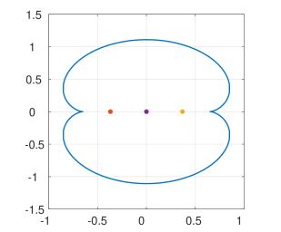
For quadrature domains of this type, Aharonov and Shapiro have proved uniqueness in [2]; in fact is determined as the image of under the conformal map . The boundary is a cardioid with a cusp at , see Fig. 2.
Let us now construct a similar q.d. but only using point charges,
Clearly both and have area . We shall choose the parameter real, such that the boundary of has a cusp.
Since the parameters in (3) must be real in this case, the conformal map takes the form
| (6) |
where and , the pre-image of , and .
Writing , we find that there is a unique choice of producing a cusp, namely
The remaining parameters in the mapping function may be obtained by solving the system corresponding to (6) using the method of “RCTD” described in Section 4. The result is
This gives a cusp at .
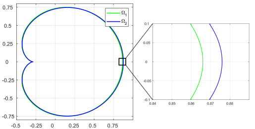
A translate of by leads to a domain having a cusp at the point and satisfying the quadrature identity
The resemblance between and (Fig. 2) is striking, even though they admit completely different quadrature identities. The similarity between and indicates that their potentials should be similar, and in terms of numerical values they are. But there is one essential difference between the two: the potential of is exactly determined by two terms in its multipole expansion while the potential for needs the entire infinite series. In detail we have
and for comparison note . From this example we see that two very similar domains may have fundamentally different potentials.
2. The master formula
As previously stated, Theorem 1.2 appears (in equivalent form) in [15, Eq. (14.12)]. We shall here give a different derivation.
Consider the univalent map normalized by and where and where the distribution is assumed to be of compact support in . Our point of departure is Poisson’s equation
Taking the distributional -derivative of we obtain the Cauchy transform
where denotes the Cauchy kernel and . Since , (2) says that . In particular is holomorphic on . Taking in the quadrature identity (1) we see that
| (7) |
In fact, an application of Bers’ approximation theorem from [4] shows that (7) is equivalent to (1). Now consider the “Schwarz potential” defined by
which is zero for . Using the continuity of we get also on . Moreover, Poisson’s equation gives on . Hence the function
is holomorphic on and continuous up to the boundary , while satisfying for . This determines as the Schwarz function for the boundary curve , cf. [15, 40].
Lemma 2.1.
The conformal mapping extends holomorphically across to an analytic function on the disk for some .
Proof.
As we saw above, the function is defined and holomorphic in some annulus , continuous up to the boundary and satisfies when . Likewise, the function is holomorphic in and continuous up to the boundary, and we have the relation
Now, is holomorphic in the exterior of , so the above formula shows that the functions and are analytic continuations of each other across the circle . In particular, is analytically continuable inwards across , which means that as well as are analytically continuable outwards across , to some disc with . ∎
Lemma 2.2.
We have that
Remark.
For an absolutely continuous measure , we prefer to denote its Cauchy transform by rather than .
Proof of Lemma 2.2.
Fix a point and a positive number and put
Set , where by Lemma 2.1. Inserting the expansion we find that
Since we may pass to the limit as , leading to
The proof of the lemma is complete. ∎
Proof of Theorem 1.2.
Given an arbitrary we define a function by
The identity (8) can be written as
| (9) |
Now fix a point and choose to be the Cauchy-kernel . With this choice, (9) takes the form
By Lemma 2.2 this is equivalent to
Taking complex-conjugates and considering the analytic continuation to we obtain
| (10) |
as desired.
We conclude this section with three examples of applications of Theorem 1.2, which are known from the literature on quadrature domains.
Example 2.1.
Given such a , we put and note that is the Schwarz function for . In view of (11), is a meromorphic function with simple poles at . As the dominant term in satisfies
From this we get that (as )
The residues of are thus just Res for all . Since on , an application of Green’s theorem and the Residue theorem now gives
where is the positively oriented boundary of . We have shown again that .
We remark that a similar proof applied to a more general point functional gives the well known result (see [26, Theorem 3.3.1]) that a solid domain is a quadrature domain of finite order if and only if each conformal map is a rational function, if and only if the Schwarz function of extends to a meromorphic function in .
Example 2.2.
Let be a linear combination of a monopole and a dipole at the origin, i.e. . The action of the pullback is then given by
Applying Theorem 1.2, we find that a normalized conformal map , where , must satisfy
Hence is a polynomial of degree two. To determine this polynomial, we need to determine the derivatives , . The computation is postponed to Subsection 5.1, after we have discussed some algebraic prerequisites.
Example 2.3.
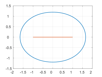
Following Davis [15, pp. 162-166] we now take be a line charge with linear density on the segment of the -axis, i.e.,
Suppose that ; the pullback by is then given by
Applying Theorem 1.2 we see that must satisfy the functional equation (cf. [15, Eq. (14.25)])
In particular, if we specialize to a uniform line charge , we obtain
This relation was found by Davis (see Eq. (14.13)), where it is also shown that if then . It is then easy to see that the above map is well-defined by choosing the standard branch of the logarithm. We have shown that there exists a unique solid domain in the class ; a picture is given in Figure 3.
3. Schur-Cohn’s test
As stated earlier, the mapping problem (3) may have non-univalent solutions . The Schur-Cohn test provides a convenient way of discarding such that fail to be locally univalent. One might hope that this procedure would leave us with at most one univalent , thus settling the uniqueness problem. As we will see later, this is indeed the case for a large class of examples.
The Schur-Cohn test is well known and quite elementary, see [28]. For reasons of completeness, we have found it convenient to briefly review the main ideas behind it here. In what follows, we let denote the space of all polynomials of degree at most ,
Lemma 3.1.
If then
(i) if then for all with ,
(ii) if then .
Proof.
(i) If then for , so .
(ii) Assume for all with . Then which leads to two cases: (1) if then obviously ; (2) if we have where are the zeros of . But then and thus since for . ∎
For each the reciprocal polynomial is defined by
Let us now define the Schur transform, by
We note a few simple facts pertaining to these objects.
First, on . Moreover, every zero of on is also a zero of and is thus a zero of . Finally,
We now construct a chain of polynomials starting with and then taking successive Schur transforms,
The last polynomial is an element in and thus is a constant.
Lemma 3.2.
If has no zeros on the unit circle and , then and have equally many zeros in .
Proof.
Let . Then and so . Since on we have on and thus Rouché’s theorem implies that and have equally many zeros in . ∎
We are now ready to formulate Schur-Cohn’s test (e.g. [28]).
Theorem 3.1.
A polynomial has no zeros in if and only if for
Proof.
Assume that has no zeros in . By Lemma 3.1, . Since has no zeros on , Lemma 3.2 implies that and has the same number of zeros in , i.e., none. If we can repeat the reasoning with instead of and deduce and so on, and after a finite number of steps we finally get .
To prove the reverse implication, assume that for . Then is a nonzero constant, and especially has no zeros on . Since , has no zeros on and by Lemma 3.2, and have the same number of zeros in , i.e., none. We may now repeat this with instead of and deduce that has no zeros in and so on, and after a finite number of steps we finally get that has no zeros in . ∎
4. Real Comprehensive Triangular Decomposition
The method of real triangular decompositions, introduced recently in [7, §4], [5, §10] and [6], provides a suitable framework to deal with the the mapping problem for quadrature domains, in the form of systems such as (4), (5). These methods in turn make use of the idea of a Cylindrical Algebraic Decomposition [3, §5], for an overview of this and other applicable methods from real algebraic geometry see, for example, the book [3].
The objects we consider here are semi-algebraic sets, given a list of polynomial equations and inequalities in a basic semi-algebraic set is the set of all points in which simultaneously satisfy all these equations and inequalities, [3, §3]. In this section we will specifically consider semi-algebraic systems defined by polynomials in the polynomial ring
where we think of the as parameters and the as variables.
More precisely, given polynomials and in , we define the semi-algebraic system to be the following set of equations and inequalities
| (12) |
The set of real solutions to (12) is called the (parameterized) semi-algebraic set generated by the system, denoted by . Moreover, for fixed we define the specialized semi-algebraic set as the set of points which satisfy the system (12) for the particular parameter-value .
Now suppose that is a collection of semi-algebraic systems in . We extend the definitions of semi-algebraic set and specialization to a parameter value by
Moreover, given a semi-algebraic system we define the constructible set of to be the set of complex solutions to the system of equations and inequalities
| (13) |
We denote by the set of solutions to (13); given we define the associated specialization to be the set of points such that .
If is a finite collection of semi-algebraic systems, it should now be obvious how to extend our definitions of constructible set () and specializations ().
A semi-algebraic system is called square-free if all polynomials and occurring in are square-free. (A polynomial is square-free if it has no factor of the form where is non-constant.)
Definition 4.1.
Let be a semi-algebraic system defined by polynomials and in and let be the associated semi-algebraic set.
A real comprehensive triangular decomposition (RCTD) of is a pair where is a finite partition of into non-empty semi-algebraic sets (called “cells”) and for each , is a finite set of square-free semi-algebraic systems such that exactly one of the following holds:
-
(1)
is empty so and for all ,
-
(2)
The specialized constructible set is infinite for all ,
-
(3)
is a finite set of semi-algebraic systems satisfying the following conditions:
-
•
is finite and has fixed cardinality for all ,
-
•
the specialized semi-algebraic sets are finite and non-empty for all and further for a fixed the specialized semi-algebraic set has fixed cardinality for all ,
-
•
for all .
-
•
The following proposition summarizes the results about RCTD’s that we will apply in the sequel.
Proposition 4.1 (§10 of [5]).
Let and be polynomials in the polynomial ring defining a semi-algebraic system . Then a real comprehensive triangular decomposition of exists and may be computed by an explicit algorithm which is guaranteed to terminate in finite time. This algorithm is implemented in the RegularChains Maple package [31].
Example 4.1.
Define and where denote real variables and denote real parameters. Consider the semi-algebraic system
Using the RegularChains package, the parameter space is partitioned into five cells where
These cells are illustrated in Figure 4.
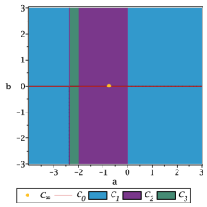
It is not hard to show that the specialized semi-algebraic set consists of points for all where ; for the cell the RCTD guarantees only that the specialized constructible set associated to the parameter choice has infinitely many points (a corresponding specialized semi-algebraic set may be infinite, empty, or finite). Hence , along with the associated semi-algebraic systems for each parameter cell, gives a RCTD of .
In more detail; consider the cells and . The disjoint union of these cells is the line (i.e. the a-axis in Figure 4). Along this line the semi-algebraic system simplifies to
| (14) |
Solving for we obtain and , so has a real solution if and only if , so . The corresponding specialized constructible set is
which is infinite. However since is never satisfied the semi-algebraic set is empty. On the other hand in the cell it is clear that the semi-algebraic system (14) has no real solutions, since when .
Now consider the subset of the cell consisting of all where and . For the system simplifies to
| (15) |
Clearly the system (15) has precisely two solutions for any , namely and . Similarly all other choices of yield associated specialized semi-algebraic sets with exactly two points.
5. Some Computational Results
In this section we apply the method of real comprehensive triangular decompositions to obtain (new) proofs of uniqueness for certain families of quadrature domains.
5.1. Aharonov-Shapiro 1976
In this subsection, we shall give an alternative proof of a theorem of Aharonov and Shapiro from [2], which states that a solid quadrature domain obeying a quadrature identity of the form
| (16) |
is unique. Here is the area of , so necessarily . The constant is allowed to be an arbitrary complex number.
Recall that the computations in Example 2.2 show that a normalized mapping function is necessarily a polynomial of degree at most , which solves the system
| (17) |
It remains to show that this system gives rise to a unique univalent solution. For this, we write
We now obtain the following semi-algebraic system, which is equivalent to (17),
We must verify that the system gives rise to at most one univalent solution for all relevant choices of quadrature data. For this, we first recognize that the last condition in is just the Schur-Cohn constraint (see Theorem 3.1), which ensures that in . In general this is only necessary for univalence but for polynomials of degree two it is also sufficient. We shall treat as parameters. Computing a real comprehensive triangular decomposition of the system , using the RegularChains library, we obtain a partition of the parameter space into two cells having the following properties.
All points in the cell are such that ; hence no point of can correspond to a quadrature domain. With , the cell is expressed as the disjoint union of the following six subsets of ,
-
(i)
-
(ii)
-
(iii)
-
(iv)
-
(v)
-
(vi)
For in each of these sets, we now prove that the system (17) has a unique solution with . Indeed, straightforward calculations show that in each of the parameter-domains, (i)–(vi) the semi-algebraic system simplifies to, respectively,
-
(i)
-
(ii)
-
(iii)
-
(iv)
-
(v)
-
(vi)
In each case (i)–(vi), we have a unique solution where , which concludes our automated proof of uniqueness for solid q.d.’s obeying (16). ∎
Remark.
The uniqueness problem for quadrature domains of order has been completely settled, see [19, Corollary 10.1]. More precisely, counting also non simply connected domains and combining with results in [20], a given point functional of order can give rise to at most two quadrature domains: one simply connected , and possibly another one of the form where is a “special point”, i.e., where is the Schwarz function. The term “special point” is due to Shapiro in [39], see Theorem 2.9 and the discussion that precedes it.
These methods can also be applied to polynomials of higher degree. (This topic is being considered as part of an ongoing work by the two of the authors.)
5.2. Symmetric smash sums
Consider a domain that satisfies
| (18) |
where and are constants and is a positive integer.
A domain satisfying (18) may be constructed as a potential theoretic sum (or “smash sum”) of discs , where excess mass coming from overlapping discs is swept out using the process of partial balayage. When this process gives rise to the well-known Neumann’s oval.
For one can surmise that a (connected) domain satisfying (18) should be either simply connected or doubly connected, depending on whether or not . The doubly connected case has already been treated in [43, Section 5.8] and in [9]. (See Subsection 7.3 for further remarks in this connection.)
In this subsection, we shall focus on the simply connected case and show how uniqueness of the quadrature domain follows using our general algebraic scheme. (In this particular case, there are, of course, alternative ways to see this, e.g. by Novikov’s theorem, Theorem 1.1, (i).)
Due to the symmetry of (18), the conformal map attains the simple form
| (19) |
where , . This gives
| (20) |
The two unknowns, and ( and ) satisfy
We only need to check solutions which are locally univalent. From (20) (or from Schur-Cohn’s test) one may easily deduce that local univalence holds if . Taking this into consideration we obtain the following semi-algebraic system
| (21) |
When setting up a real comprehensive triangular decomposition, we cannot treat as a parameter but have to use a fixed value of (since if is treated as a parameter the system (21) is no longer semi-algebraic). Below we show the results for but the corresponding decompositions may be obtained for up to without any runtime issues.
Thus let be the semi-algebraic system (21) with fixed. The associated semi-algebraic set is contained in . We treat as parameters and consider the specialized semi-algebraic set . Using an RCTD, we have found that the parameter space is divided into two cells such that for all the system has precisely one real solution and for all the system has no real solutions. The cell is made up of the three regions defined in (i), (i), and (iii) below.
-
(i)
-
(ii)
-
(iii)
In each of the domains above, the semi-algebraic system (21) simplifies as follows
-
(i)
-
(ii)
-
(iii)
Since for all choices of the parameters in the cell we know from the definition of the RCTD that the number of real solutions is fixed, picking a particular and in it is easy to verify that the systems above have unique real solutions which correspond to a quadrature domain. Similarly, one can pick a choice of parameters in to verify that the system (21) has no real solutions for any parameter choice in . In particular, we have shown that a quadrature domain obeying a quadrature identity (18) is uniquely determined. However, we cannot yet be sure that each solution to the system (21) defines a univalent map since we have only required local univalence. The following proposition shows that this is in fact the case.
Proposition 5.1.
The mapping in (19), (), is univalent if and only if
| (22) |
Proof.
The necessity is obvious since the strict inequality is just the Schur-Cohn condition for to have no zeros in .
To prove sufficiency we shall prove that (22) implies that is starlike, and in particular univalent. Recall ([34, Theorem 2.5]) that starlikeness is equivalent to that for all . Using the Cauchy-Riemann equations one finds that this is equivalent to
(Cf. [16]). Using Eq. (19) we find that is a positive multiple of
| (23) |
This is a quadratic polynomial in which is clearly positive when . We need to prove that it remains positive for all with if and (22) holds. We may assume that and . For odd , the non-negativity of (23) then means
| (24) |
while for even , it means
| (25) |
By assumption , so the inequalities (24), (25) amount to and respectively. This is equivalent to and proves that is starlike if and only if (22) holds. ∎
6. Three examples of uniqueness
In this section we give several further examples of uniqueness of quadrature domains based on real comprehensive triangular decomposition and other computational methods from algebraic geometry (i.e. Gröbner basis computations).
Example 6.1.
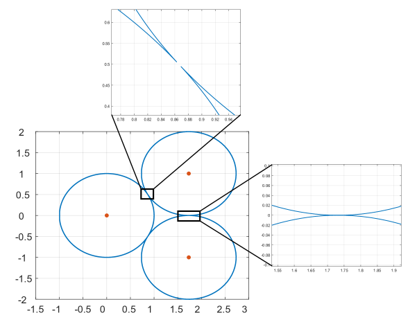
Let be a quadrature domain satisfying
| (26) |
the nodes are chosen such that the union is just barely simply connected (this is guaranteed by ), see Fig. 5.
To find the mapping we need to solve the six complex equations , or equivalently 12 real equations. Without loss of generality we pick and , moreover, using the mirror symmetry in (26) we get and . This means that in total we only have to solve for five real variables. The equations are of course rational, meaning that in order to calculate the Gröbner basis we need to clear denominators and algebraically remove the new roots introduced by this. These new roots correspond to poles of the original rational system, and hence are not of interest. The defining equations without roots at the poles are obtained by saturating the resulting ideal by the product of the equations from the denominators.
A Gröbner basis calculation shows that there is a unique solid quadrature domain obeying (26), depicted in Fig. 5. To be explicit, we can write and , where
Note that the values above can be obtained as exact expressions in a field extension of from the result of our Gröbner basis computation, however we opt to give the numerical approximations here for simplicity.
Example 6.2.
Let and let be a quadrature domain satisfying
This is similar to a -symmetric domain in Subsection 5.2, but with an additional node at the origin. Assuming is simply connected, the mapping is given by
where and . Clearing denominators leads to the semi-algebraic system
| (27) |
with variables and parameter .
 |
 |
 |
 |
 |
 |
Let denote the semi-algebraic system (27). Computing a triangular decomposition yields two cells: and in the parameter space (with coordinate ). For each the system has no real solutions while for each the system has exactly one real solution ; note that .
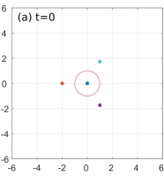
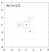
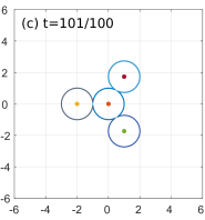
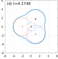
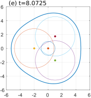
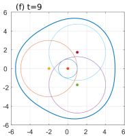
Observe that to obtain a solution, we must have in order that be simply connected (see Fig. 6(c)). If we interpret as time, we may think of the quadrature domain as the result of a Hele-Shaw evolution, starting from , after injecting fluid through the nodes at constant rate , for units of time (see Subsection 7.2 below for more about this). The evolution is depicted in Fig. 6.
Example 6.3.
Let be a quadrature domain satisfying
| (28) |
This is a - symmetric domain with as in Subsection 5.2 but with negative weights and an additional node at the origin with strength two. The mapping then satisfies
where and . To obtain unique solutions for this system we have to impose Schur-Cohn constraints; this is as easily done for arbitrary as for so we do it for arbitrary .
Set where and . The derivative of the mapping is given by
When we have that and . It follows that the Schur-Cohn constraints for the case are given by
where we allow for equality to include the case where has cusps, see Fig. 7.
Clearing denominators in the equations , recalling that , , and adding the Schur-Cohn constraints we obtain the semi-algebraic system
| (29) |
where we treat as a parameter and as variables (note are fixed). Let denote the semi-algebraic system (29). Let and set
A computation of a real comprehensive triangular decomposition for gives that the parameter space (with coordinate ) is partitioned into two cells: and . For all the system has no solutions and for all the system has exactly one real solution . It follows that for any valid choice of the parameter there exists a unique quadrature domain. The parameter value corresponds to the case where has two cusps, as shown in Fig. 7.
7. Other related topics
In this section, we briefly discuss some of the existing methods and constructions in the theory of quadrature domains with bearing for our above methods. The reader interested in a comprehensive picture of the area should consult one or several of the textbooks [12, 15, 25, 26, 40, 43].
7.1. The defining polynomial of a q.d.
Consider a quadrature domain of order corresponding to a point-functional
| (30) |
It was shown by Aharonov and Shapiro in [2] that the boundary is an algebraic curve, and more precisely there exists an irreducible polynomial which is self-conjugate and normalized (i.e. , ) such that
| (31) |
where a “special point” is an isolated solution to the equation . (Cf. [39])
It is convenient to refer to the polynomial in (31) as the “defining polynomial” for the quadrature domain . A natural problem, then, is to try to characterize the set of defining polynomials which are associated with a given point-functional . This problem has been investigated by Gustafsson in [19, 20], and leads to interesting insights with respect to the uniqueness question (Q). To elucidate this, we write a defining polynomial in the form
| (32) |
where each is a polynomial of degree at most .
It is shown in [19] (cf. also [8]) that there is an explicit bijection between point-functionals (of the form (30)) and the last two polynomials which may appear in the expansion (32). As pointed out in [19, 8], the determination of the remaining polynomials is generally a difficult matter. In the simply connected case, this problem is similar to the question of completely characterizing all solutions to the master formula (in Theorem 1.2), for each point-functional .
Remark.
The notion of a special point is not just an artefact of the construction. For example, such points appear naturally in the process of forming smash sums of discs (i.e., each time discs “collide” as in Figure 6 (c)) and they have the physical interpretation of stagnation points for fluid flows. We refer to [20, 8] for further details.
7.2. Connection to Laplacian growth
Let be a real parameter and consider a family of quadrature domains , each obeying the quadrature identity
| (33) |
where is a real constant, and where we take for simplicity. If , we may think of as an expanding blob of fluid, obtained from by injecting fluid at the origin, at constant rate . (If , the domains contract due to suction.) The resulting evolution is known under the names “Hele-Shaw evolution” and “Laplacian growth”, see e.g. [1, 26, 43].
For values of such that is solid, we will write for the Riemann mapping .
Remark.
Any domain is by definition of finite order, and hence its boundary is part of an algebraic curve, see Subsection 7.1. This implies that the boundary curve is smooth everywhere with the possible exception of finitely many singular points, which may be either cusps pointing inwards (corresponding to values , at which ), or contact points (which satisfy for two distinct points ). For solid domains, contact points are excluded.
In the following, we suppose that is a smoothly varying family of solid domains obeying (33) for in some suitable time-interval. A basic result relates the “time-derivative” to the “space-derivative” .
Theorem 7.1.
The conformal map onto satisfies Polubarinova-Galin’s equation
| (34) |
A proof can be found in the book [25], Section 1.4.2.
Gustafsson and Lin in [22] have studied the evolution of zeros and poles of the space-derivative . We will now briefly indicate a different possible approach based on our basic structure theorem, Theorem 1.2. Denote by the points in such that , and write . Also denote and when . In view of (3), the mapping obeys
| (35) |
which gives
| (36) |
and (denoting complex conjugation by , and abbreviating , , etc.)
| (37) |
7.3. Multi-connected quadrature domains
A theory for multiply connected quadrature domains, using the Schottky double of the domain, is developed in the paper [19]. The mapping problem for such domains has been the subject of numerous investigations. In particular, for a significant class of quadrature domains (e.g. based on forming suitable smash sums of discs), the Riemann map can be constructed using the corresponding “Schottky-Klein prime function”. This approach is found in the works [13, 10] as well as in the recent monograph [12, Chapter 11]. (The Schottky-Klein function is surveyed in the article [11].)
Acknowledgments
This work was supported in part by the Anders Wall Foundation.
References
- [1] Ar. Abanov, M. Mineev-Weinstein, and A. Zabrodin. Multi-cut solutions of Laplacian growth. Phys. D, 238(17):1787–1796, 2009.
- [2] Dov Aharonov and Harold S. Shapiro. Domains on which analytic functions satisfy quadrature identities. Journal d’Analyse Mathématique, 30(1):39–73, Dec 1976.
- [3] Saugata Basu, Richard Pollack, and Marie-Françoise Roy. Algorithms in real algebraic geometry, volume 10. Springer, 2006.
- [4] Lipman Bers. An approximation theorem. J. Analyse Math., 14:1–4, 1965.
- [5] Changbo Chen. Solving polynomial systems via triangular decomposition. PhD thesis, The University of Western Ontario, 2011.
- [6] Changbo Chen, Oleg Golubitsky, François Lemaire, Marc Moreno Maza, and Wei Pan. Comprehensive triangular decomposition. In International Workshop on Computer Algebra in Scientific Computing, pages 73–101. Springer, 2007.
- [7] Changbo Chen and Marc Moreno Maza. Semi-algebraic description of the equilibria of dynamical systems. In International Workshop on Computer Algebra in Scientific Computing, pages 101–125. Springer, 2011.
- [8] Darren Crowdy. Multipolar vortices and algebraic curves. R. Soc. Lond. Proc. Ser. A Math. Phys. Eng. Sci., 457(2014):2337–2359, 2001.
- [9] Darren Crowdy. The construction of exact multipolar equilibria of the two-dimensional Euler equations. Phys. Fluids, 14(1):257–267, 2002.
- [10] Darren Crowdy. Quadrature domains and fluid dynamics. In Peter Ebenfelt, Björn Gustafsson, Dmitry Khavinson, and Mihai Putinar, editors, Quadrature Domains and Their Applications, pages 113–129, Basel, 2005. Birkhäuser Basel.
- [11] Darren Crowdy. The Schottky-Klein prime function on the Schottky double of planar domains. Comput. Methods Funct. Theory, 10(2):501–517, 2010.
- [12] Darren Crowdy. Solving Problems in Multiply Connected Domains. NSF-CBMS Regional Conference Series in Applied Mathematics: 97. SIAM, Philadelphia USA, 2020.
- [13] Darren Crowdy and Jonathan Marshall. Constructing multiply connected quadrature domains. SIAM J. Appl. Math., 64(4):1334–1359, 2004.
- [14] Philip J. Davis. Double integrals expressed as single integrals or interpolatory functionals. J. Approximation Theory, 5:276–307, 1972.
- [15] Philip J. Davis. The Schwarz function and its applications. The Mathematical Association of America, Buffalo, N. Y., 1974. The Carus Mathematical Monographs, No. 17.
- [16] Fejér, L. and Szegö, G. Special conformal mappings. Duke Math. J., 18(2):535–548, 06 1951.
- [17] Stephen J. Gardiner and Tomas Sjödin. Convexity and the Exterior Inverse Problem of Potential Theory. Proceedings of the American Mathematical Society, 136(5):1699–1703, 2008.
- [18] Stephen J. Gardiner and Tomas Sjödin. A characterization of annular domains by quadrature identities. Bull. Lond. Math. Soc., 51(3):436–442, 2019.
- [19] Björn Gustafsson. Quadrature identities and the Schottky double. Acta Appl. Math., 1(3):209–240, 1983.
- [20] Björn Gustafsson. Singular and special points on quadrature domains from an algebraic geometric point of view. J. Analyse Math., 51:91–117, 1988.
- [21] Björn Gustafsson. On quadrature domains and an inverse problem in potential theory. J. Analyse Math., 55:172–216, 1990.
- [22] Björn Gustafsson and Yu-Lin Lin. On the dynamics of roots and poles for solutions of the Polubarinova-Galin equation. Ann. Acad. Sci. Fenn. Math., 38(1):259–286, 2013.
- [23] Björn Gustafsson, Yu-Lin Lin, and Joakim Roos. Laplacian growth on branched riemann surfaces. To Appear.
- [24] Björn Gustafsson and Harold S. Shapiro. What is a quadrature domain? In Quadrature domains and their applications, volume 156 of Oper. Theory Adv. Appl., pages 1–25. Birkhäuser, Basel, 2005.
- [25] Björn Gustafsson and Alexander Vasil’ev. Conformal and Potential Analysis in Hele-Shaw Cell. Advances in Mathematical Fluid Mechanics. Birkhäuser Verlag, 2006.
- [26] Björn Gustafsson, Alexander Vasil’ev, and Razvan Teodorescu. Classical and stochastic Laplacian growth. Advances in Mathematical Fluid Mechanics. Springer, 2014.
- [27] Björn Gustafsson and Mihai Putinar. Selected topics on quadrature domains. Physica D: Nonlinear Phenomena, 235(1):90 – 100, 2007. Physics and Mathematics of Growing Interfaces.
- [28] Peter Henrici. Applied and computational complex analysis. Vol. 1. Wiley Classics Library. John Wiley & Sons, Inc., New York, 1988. Power series—integration—conformal mapping—location of zeros, Reprint of the 1974 original, A Wiley-Interscience Publication.
- [29] Victor Isakov. Inverse source problems. Mathematical surveys and monographs: 34. American Mathematical Society, 1990.
- [30] Seung-Yeop Lee and Nikolai G. Makarov. Topology of quadrature domains. J. Amer. Math. Soc., 29(2):333–369, 2016.
- [31] F. Lemaire, M. Moreno Maza, and Y. Xie. The RegularChains library. In I. Kotsireas, editor, Proceedings of Maple Conference, pages 355–368. Maplesoft, 2005.
- [32] M. B. Mineev. A finite polynomial solution of the two-dimensional interface dynamics. Phys. D, 43(2-3):288–292, 1990.
- [33] Par P Novikoff. Sur le problème inverse du potentiel. Comptes Rendus (Doklady) de l’Académie des Sciences de l’URSS, 18(3):165–168, 1938.
- [34] Christian Pommerenke. Univalent functions. Vandenhoeck & Ruprecht, Göttingen, 1975. With a chapter on quadratic differentials by Gerd Jensen, Studia Mathematica/Mathematische Lehrbücher, Band XXV.
- [35] M. Sakai. Linear combinations of harmonic measures and quadrature domains of signed measures with small supports. In Proceedings of the Edinburgh Mathematical Society, volume 42, pages 433–444, 1999.
- [36] Makoto Sakai. Quadrature Domains. Springer Verlag, 1982.
- [37] Makoto Sakai. Finiteness of the family of simply connected quadrature domains. In Potential theory (Prague, 1987), pages 295–305. Plenum, New York, 1988.
- [38] Makoto Sakai. Sharp Estimates of the Distance from a Fixed Point to the Frontier of a Hele-Shaw Flow. Potential Analysis, 8(3):277–302, May 1998.
- [39] Harold S. Shapiro. Unbounded quadrature domains. In Complex analysis, I (College Park, Md., 1985–86), volume 1275 of Lecture Notes in Math., pages 287–331. Springer, Berlin, 1987.
- [40] Harold S. Shapiro. The Schwarz function and its generalization to higher dimensions, volume 9 of The University of Arkansas lecture notes in the mathematical sciences. Wiley, 1992.
- [41] Brian Skinner. Logarithmic Potential Theory on Riemann Surfaces. ProQuest LLC, Ann Arbor, MI, 2015. Thesis (Ph.D.)–California Institute of Technology.
- [42] Carina Ullemar. A uniqueness theorem for domains satisfying a quadrature identity for analytic functions. Technical Report TRITA-MAT-1980-37, KTH Royal Institute of Technology, 1980.
- [43] A. N. Varc̆enko and P. I. Etingof. Why the boundary of a round drop becomes a curve of order four. University lecture series: 3. American Mathematical Society, 1992.
- [44] Lawrence Zalcman. Some inverse problems of potential theory. In Integral geometry (Brunswick, Maine, 1984), volume 63 of Contemp. Math., pages 337–350. Amer. Math. Soc., Providence, RI, 1987.
- [45] D Zidarov. Method of finding point (dipole) solutions of the potential field inverse problem. pure and applied geophysics, 110(1):1918–1926, 1973.
- [46] D Zidarov and Zh Zhelev. On obtaining a family of bodies with identical exterior fields-method of bubbling. Geophysical Prospecting, 18(1):14–33, 1970.