Deep Learning-based Image Compression with
Trellis Coded Quantization

Abstract

Recently many works attempt to develop image compression models based on deep learning architectures, where the uniform scalar quantizer (SQ) is commonly applied to the feature maps between the encoder and decoder. In this paper, we propose to incorporate trellis coded quantizer (TCQ) into a deep learning based image compression framework. A soft-to-hard strategy is applied to allow for back propagation during training. We develop a simple image compression model that consists of three subnetworks (encoder, decoder and entropy estimation), and optimize all of the components in an end-to-end manner. We experiment on two high resolution image datasets and both show that our model can achieve superior performance at low bit rates. We also show the comparisons between TCQ and SQ based on our proposed baseline model and demonstrate the advantage of TCQ.

1 Introduction

The goal of designing the optimal image codec is to minimize the distortion $D$ between the original image and the reconstructed image subject to the constraint of the bitrate $R$. As the entropy $H$ is the lower bound of bitrate $R$, the optimization can be formulated as minimizing $D+\lambda H$, where $\lambda>0$ is the tradeoff factor. Recently many works [1, 2, 3] attempt to develop image compression models based on deep learning architectures. In their approaches, a uniform scalar quantizer (SQ) is commonly applied to the feature maps between the encoder and decoder. As the codewords are distributed in a cubic and the corresponding Voronoi regions induced by SQ are always cubic, SQ cannot achieve the R-D bound [4]. Vector quantization (VQ) has the optimal performance, but the complexity is usually high. Trellis coded quantizer (TCQ) is a structured VQ, and it can achieve better performance than SQ with modest computational complexity [5]. It is shown in [5] that for memoryless uniform sources, a 4 state TCQ can achieve 0.87dB higher SNR than SQ for 4 bit$/$sample.

In this paper, motivated by the superior performance of TCQ over SQ in traditional image coding, we propose to use TCQ to replace the commonly used SQ in a deep learning based image compression model. The soft-to-hard strategy [6] is applied to allow for back propagation during training. To the best of our knowledge, we are the first to investigate the performance of TCQ in a deep learning based image compression framework. Our implementation allows for batch processing amenable to the mini-batch training in deep learning models, which greatly reduces the training time.

The entropy coding can further reduce the bitrate without impacting the reconstruction performance. One way to apply it in deep learning model is to use offline entropy coding method during testing [7]. This method is not optimized for the bitrate as the network is not explicitly designed to minimize the entropy. In this paper, we adopt the PixelCNN++ [8] to model the probability density function on an image $x$ over pixels from all channels as $p(x)=\prod_{i}p(x_{i}|x_{<i})$, where the conditional probability only depends on the pixels above and to the left of the pixel in the image. A cross entropy loss is followed to estimate the entropy of the quantized representation to jointly minimize the R-D function.

Our contributions are summarized as follows. We propose to incorporate TCQ into a deep learning based image compression framework. The image compression framework consists of encoder, decoder and entropy estimation subnetworks. They are optimized in an end-to-end manner. We experiment on two commonly used datasets and both show that our model can achieve superior performance at low bit rates. We also compare TCQ and SQ based on the same baseline model and demonstrate the advantage of TCQ.

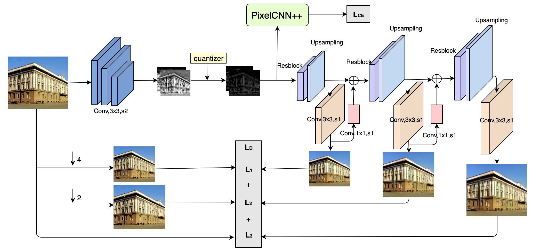
Figure 1: Overview of our proposed deep image compression model. The encoder has three consecutive strided convolutional layers to reduce the input size from 256$\times$256 to 32$\times$32. After the TCQ is applied, the quantized feature representations are used as input to two branches. One goes to the decoder network to generate image from resolution 64$\times$64 to 128$\times$128, and then to 256$\times$256. These three losses are added together to be the distortion loss $L_{D}$. The other one goes to the entropy model (pixelCNN++) to produce the probability matrix of pixels based on previous pixels optimized by the cross entropy loss $L_{CE}$. “Conv, $a\times a$, sb” denotes convolutional layer with $a\times a$ kernels and a stride of b. “Resblock” is from [9] but without BatchNorm layers. “$\downarrow$c ” represents downsampling by a factor of c.

2 Related Work

There has been a line of research on deep learning based image compression, especially autoencoders with a bottleneck to learn compact representations. The encoder maps the image data to the latent space with reduced dimensionality, and the decoder reconstructs the original image from the latent representation.

2.1 Quantization in DNN

Several approximation approaches have been proposed to allow the network to back-propagate through the quantizer during training. In [10, 11], a binarization layer is designed in the forward pass and the gradients are defined based on a proxy of the binarizer. Ballé et. al. [1] stochastically round the given values by adding noise and use the new continuous function to compute the gradients during the backward pass. Theis et. al. [2] extend the binarizer in [10] to integers and use straight-through estimator in the backward pass. In [6], a soft quantization in both forward and backward passes is proposed. The model needs to learn the centers and change from soft quantization to hard assignments during training by an annealing strategy. In [3], the authors apply the nearest neighbors to obtain fixed centers, and the soft quantization in [6] is used during the backward pass.

2.2 Image Compression based on DNN

With the quantizer being differentiable, in order to jointly minimize the bitrate and distortion, we also need to make the entropy differentiable. For example, in [1, 2], the quantizer is added with uniform noise. The density function of this relaxed formulation is continuous and can be used as an approximation of the entropy of the quantized values. In [6], similar to the soft quantization strategy, a soft entropy is designed by summing up the partial assignments to each center instead of counting. In [3, 11], an entropy coding scheme is trained to learn the dependencies among the symbols in the latent representation by using a context model. These methods allow jointly optimizing the R-D function.

3 Proposed Approach

Our model follows the encoder-decoder framework. Different from the previous works that apply a uniform scalar quantizer (SQ) after the encoder network, we propose to use trellis coded quantizer (TCQ) to enhance the reconstruction performance. The whole framework is trained jointly with our entropy model.

3.1 Encoder and Decoder

Since our goal is to study the gain of TCQ and SQ, we only use a simple encoding and decoding framework. Our encoder network consists of three layers of convolutional layers with a stride of 2 to downsample the input. Each convolutional layer is followed by a ReLU layer. We remove BatchNorm [12] layers as we find removing them gives us better reconstruction performance. We add one more convolutional layer to reduce the channel dimension to a small value e.g. 8 to get a condensed feature representation $F$. A $Tanh$ layer is followed to project $F$ to continuous values between -1 and 1. Then a quantizer is applied to quantize the feature maps to discrete values. For the decoder network, we use PixelShuffle [13] layer for upsampling. Inspired by [14], we adopt two intermediate losses after each upsampling operation to force the network to generate images from low resolution to high resolution progressively as shown in Fig. 1.

3.2 Trellis Coded Quantizer

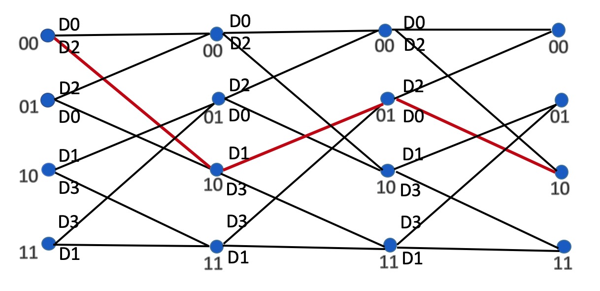
Figure 2: An example of 4 state trellis structure.

(a)	(b)	(c)

Figure 3: (a) indexing method I for TCQ, (b) indexing method II for TCQ, (c) SQ.

Forward Pass: Trellis coded quantizer (TCQ) is applied in JPEG2000 [4] part II. Different from JPEG2000 where the input for TCQ is fixed given an image block, when embedded in deep neural networks, the input for TCQ is updated in each iteration during training. The forward pass for TCQ is similar to the original implementation in [4]. In essence, TCQ aims to find a path with minimum distortion from the start symbol to the last symbol based on the particular diagram structure. Figure 3 shows a trellis structure with 4 states. For $R$ bit/symbol, a quantizer with $2^{R+1}$ quantization levels is created. These $2^{R+1}$ reconstruction points can be obtained by a uniform quantizer. As the last layer of our encoder is a $Tanh$ function, we have $V_{max}=1$ and $V_{min}=-1$. The quantization step is $\Delta=\dfrac{2}{2^{R+1}}$. A reconstruction point $c_{j}$ ($j=1,2,\cdots,2^{R+1}$) is obtained by $c_{j}=-1+\Delta/2+(j-1)\times\Delta$. Next all the reconstruction levels are partitioned into four subsets ${D_{0},D_{1},D_{2},D_{3}}$ from left to right to form four sub-quantizers. Then different subsets are assigned to different branches of the trellis, so that different paths of the trellis can try different combinations to encode an input sequence. Each node only needs to record the input branch that has the smallest cost. After obtaining the minimum distortion for the last symbol, we trace back to get the optimal path as shown in red in Fig. 3 for instance. With this optimal path, 1 bit $q$ is used to indicate which branch to move for next symbol, and the last $R-1$ bits ${b_{1}b_{2}\cdots b_{R-1}}$ are used to indicate the index of codeword from the corresponding sub-quantizer. Here we call it indexing method I .

Backward Pass: In order to make a quantizer differentiable, the most common way is to use straight-through estimator [15] where the derivative of the quantizer is set to 1. However, we find that such backward method tends to converge slowly for TCQ. As the TCQ changes the distribution of the input data, this inconsistency may make it hard for the network to update weights in the right direction. Similar to [3], given reconstruction points $C=\{c_{1},c_{2},\cdots,c_{L}\}$ ($L=2^{R+1}$), we use the differentiable soft quantization during the backward pass.

$$\tilde{Q}(z)=\Sigma_{j=1}^{L}\dfrac{exp(-\sigma||z-c_{j}||)}{\Sigma_{l=1}^{L}exp(-\sigma||z-c_{l}||)}c_{j}$$ (1)

where $\sigma$ is a hyperparameter to adjust the “softness” of the quantization.

Discussions: One issue for the TCQ implementation is that the time and memory complexity are both proportional to the number of symbols. Previous implementation usually flattens the input block into a sequence. Because pixels in one feature map are more correlated than pixels in other feature maps, we consider each feature map as an input for TCQ. For feature maps with size $B\times C\times H\times W$ ($B$ is the batch size for the network, $C$ is the number of channels, $H$ and $W$ are the height and width), we reshape the size as $BC\times HW$, where $BC$ is the batch size for TCQ and $HW$ is the number of symbols in a feature map, which reduces the processing time.

The other issue is that the conventional indexing method I mentioned above brings in randomness for the indices of a feature map as shown in Fig. 3 (a). The reason is that the branch bit $q$ depends on the optimal path in trellis structure and it does not carry any relationship among each symbol. From JPEG2000 [4], we have two union-quantizers $A0={D0\bigcup D2}$ and $A1={D1\bigcup D3}$. As pointed in [16], given a node in the diagram, the codeword that can be chosen is either from $A0$ or $A1$. Therefore, because of the particular structure of the trellis, all $R$ bits can be used to represent the indices for the union-quantizer $A0$ and the same applies to $A1$. For example, in Fig. 3, assume we receive the initial state $01$ during decoding. Only $D0$ or $D2$ sub-quantizer will be chosen for this symbol. As the indices for $D0$ and $D2$ are all different, we get the corresponding unique codeword based on the received $R$ bits. Then we easily know which sub-quantizer ($D0$ or $D2$) is chosen and accordingly the branch number. We call it indexing method II. Fig. 3 (b) gives the indices of a feature map resulting from the indexing method II.

3.3 Entropy Coding Model

The aforementioned autoencoder model is not optimized for entropy coding. We can model the conditional probability distribution of a symbol based on its context [3]. The context should be only related to previous decoded symbols, and not use the later unseen symbols. We employ PixelCNN++ [8] model for the entropy coding model. We replace the last layer of PixelCNN++ model in implementation with a softmax function so that a cross entropy loss can be used during training. This loss is viewed as an estimation of entropy for the quantized latent representation. Assume we have $R$ bits to encode each symbol and a $C\times H\times W$ dimensional feature map $F$, the PixelCNN++ model outputs a $2^{R}\times C\times H\times W$ probability matrix. Encoding is done row by row and each row orders from left to right. With the probability matrix, we encoder the indices of the feature maps by Adaptive Arithmetic Coding (AAC) to get the compressed representation. During decoding, for the first forward pass, we input the pre-trained PixelCNN++ model with a tensor with all zeros. This first forward pass gives distributions for entries $p(z_{c=1:C,i=1,j=1})$ where $(c,i,j)$ is a position in the feature map $F$. Then we decode the indices along the channel dimension by AAC. Based on the received initial states, we recover the symbols at $({\small c=1:C,i=1,j=1})$. The following decoding steps are based on the conditional probability

$$p(z_{c=1:C,i=u,j=v}|Context)=\text{PixelCNN++}(T_{{\small\{1:C,1:u,1:(v-1)\}\bigcup\{1:C,1:(u-1),v:W\}}})_{c,i,j}$$ (2)

where $T_{{\small 1:x,1:y,1:z}}$ is a tensor with decoded symbol at location $\{(c,i,j)|1\leq c\leq x,1\leq i\leq y,1\leq j\leq z\}$ and zeros otherwise. When $u=1$, ${\small\{1:C,1:(u-1),v:W\}}=\O$. When $v=1$, ${\small\{1:C,1:u,1:(v-1)\}}=\O$. As the decoding proceeds, the remaining zeros will be replaced by the decoded symbols progressively.

4 Experiment

4.1 Dataset

We use ADE20K dataset [17] for training and validation. We test on Kodak PhotoCD image dataset and Tecnick SAMPLING dataset [18]. ADE20K dataset contains 20K training and 2K validation images. Kodak PhotoCD image dataset and Tecnick SAMPLING dataset include 24 512$\times$768 images and 100 1200$\times$1200 images respectively.

4.2 Training Details

We crop each input image by 256$\times$256 during training and test on the whole images. During training, we use a learning rate of 0.0001 at the beginning, and decrease it by a factor 0.4 at epoch 80, 100 and 120. Training is stopped at 140 epochs and we use the model that gives the best validation result for testing. We set the batch size as 18 and run the training on one 12G GTX TITAN GPU with the Adam optimizer. We use 4 quantization levels and increase the channel size from $\{4,6,8,12,16\}$ to control the bitrate. Compression performance is evaluated with Multi-Scale Structural Similarity (MS-SSIM) by bits per pixel (bpp) and we use MS-SSIM loss in Eq. 3 during training.

$$L_{\text{MS-SSIM}}=100(1-L_{D}(\text{MS-SSIM}(\tilde{X},X)))+\lambda L_{CE}$$ (3)

The first term is the distortion error and the second term is the cross entropy loss for pixelCNN++ model. $\lambda$ is a hyperparameter and set to 1.

4.3 Baselines

We compare our results with conventional codecs and recent deep learning based compression models. JPEG [19] results are obtained from ImageMagick. JPEG2000 results are from MATLAB implementation and BPG results are based on 4:2:0 chroma format. For deep learning based image compression models, we either collect from the released test results or plot the rate-distortion curves from the published papers.

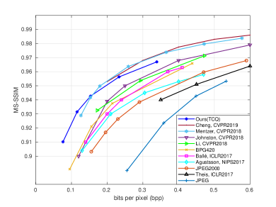
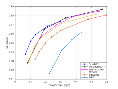
(a)	(b)

Figure 4: (a) MS-SSIM/bpp on Kodak dataset. (b) MS-SSIM/bpp on Tecnick dataset.

Table 1: Performance comparisons between TCQ and SQ using MS-SSIM loss for training

quantizer	Kodak dataset		Tecnick dataset
	PSNR(dB)/bpp	MS-SSIM/bpp	PSNR(dB)/bpp	MS-SSIM/bpp
SQ	24.54/0.077	0.9028/0.077	26.14/0.068	0.9326/0.068
TCQ	24.95/0.076	0.9102/0.076	26.82/0.066	0.9377/0.066
SQ	25.66/0.117	0.9259/0.117	27.63/0.104	0.9493/0.104
TCQ	25.85/0.116	0.9315/0.116	27.86/0.101	0.9518/0.101
SQ	26.23/0.157	0.9386/0.157	28.32/0.139	0.9572/0.139
TCQ	26.47/0.154	0.9427/0.154	28.45/0.133	0.9592/0.133

Table 2: Performance comparisons between TCQ and SQ using MSE loss for training

quantizer	Kodak dataset		Tecnick dataset
	PSNR(dB)/bpp	MS-SSIM/bpp	PSNR(dB)/bpp	MS-SSIM/bpp
SQ	24.86/0.064	0.8715/0.064	25.94/0.054	0.9091/0.054
TCQ	25.23/0.062	0.8824/0.062	26.66/0.052	0.9189/0.052
SQ	25.81/0.098	0.8992/0.098	27.35/0.081	0.9308/0.081
TCQ	26.35/0.096	0.9090/0.096	27.96/0.078	0.9373/0.078
SQ	26.56/0.133	0.9178/0.133	28.18/0.112	0.9427/0.112
TCQ	26.89/0.130	0.9232/0.130	28.65/0.110	0.9473/0.110

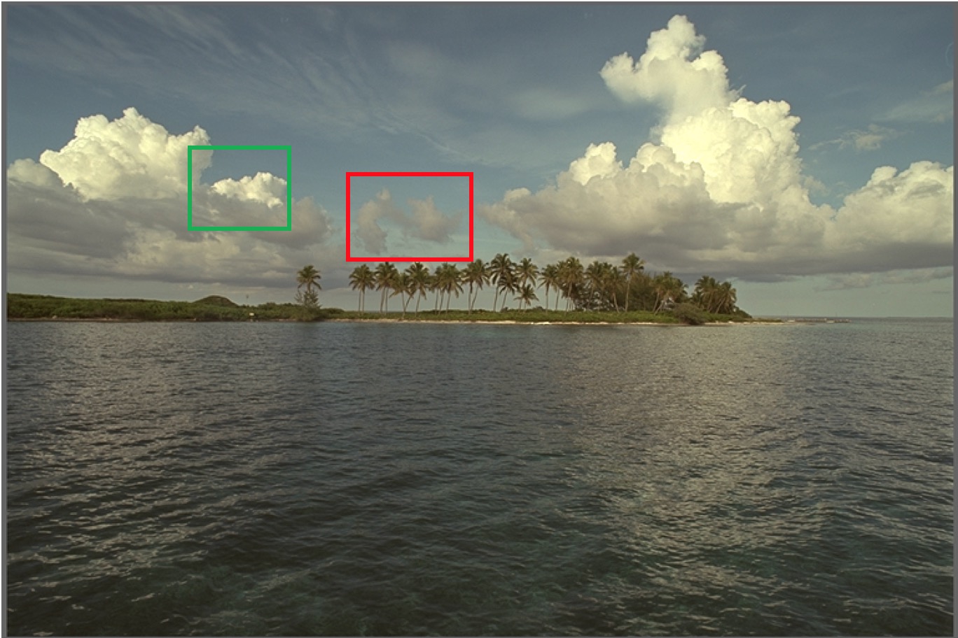
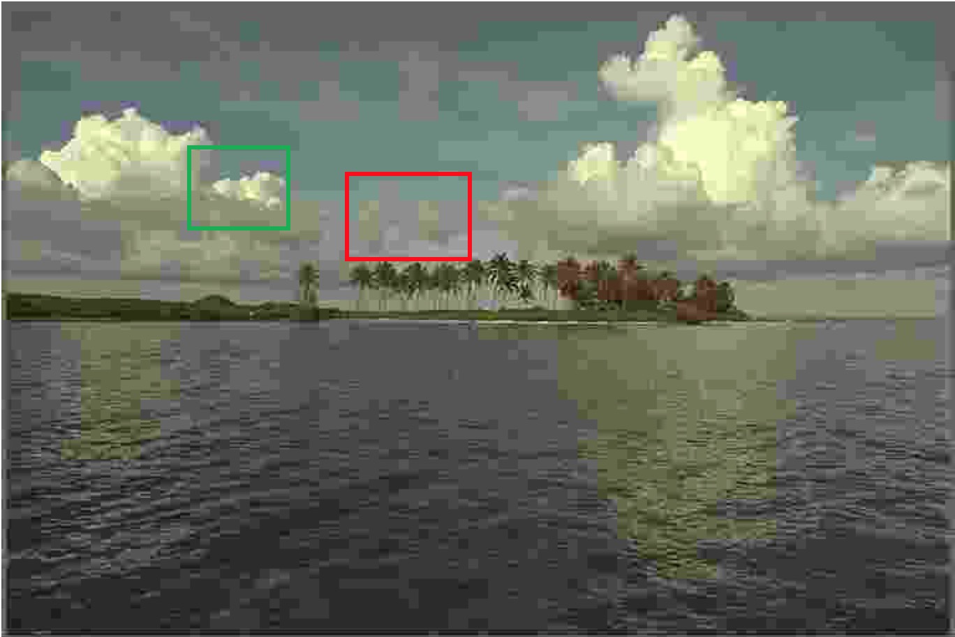
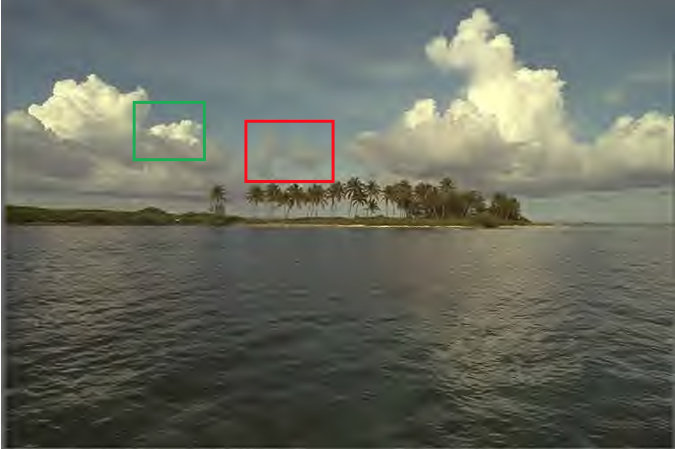
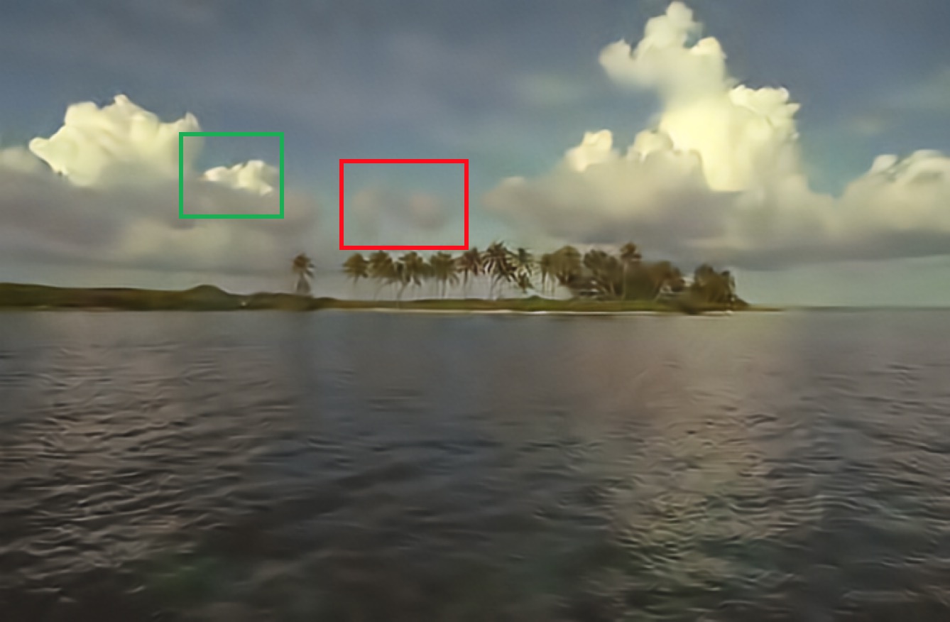
	0.8177/0.128	0.9028/0.118	0.9139/0.117
(a) Original	(b) JPEG	(c) JPEG2000	(d) Ballé [1]
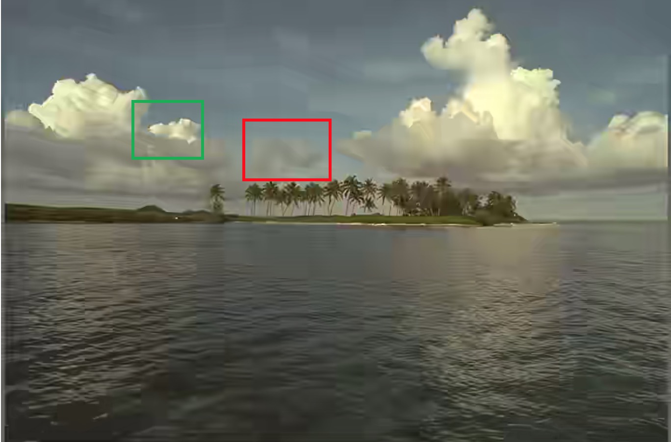
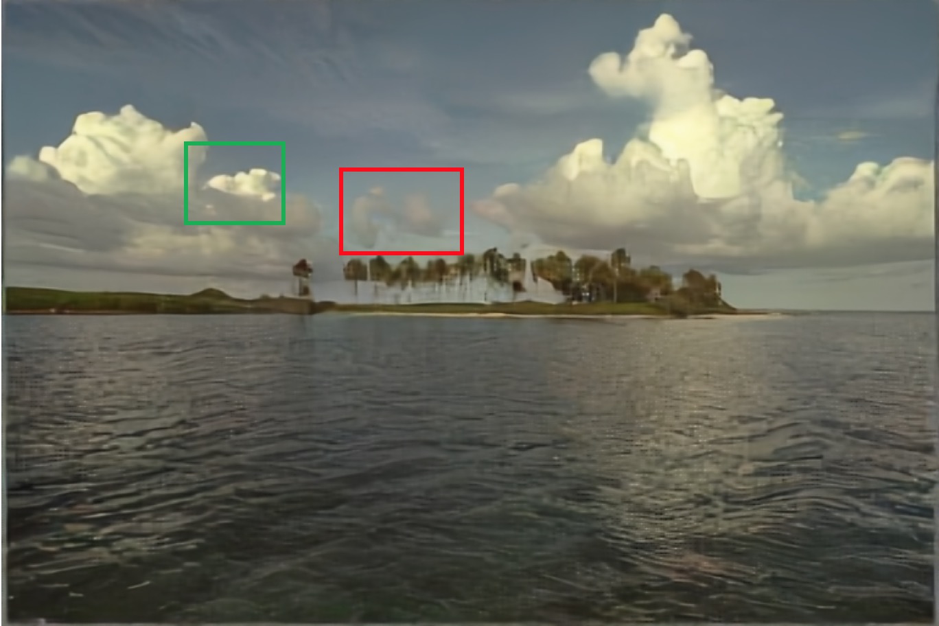
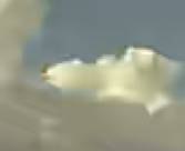
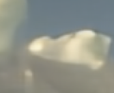
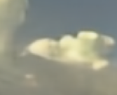
	0.9189/0.112	0.9257/0.112	0.9323/0.109
	(e) BPG	(f) Ours (SQ)	(g) Ours (TCQ)

Figure 5: Qualitative results (MS-SSIM/bpp) from the image kodim16 on kodak dataset.

4.4 Comparisons with previous works

Fig. 4 shows result comparisons between our approach and other image compression algorithms (Theis et. al. [2], Ballé et. al. [1], Agustsson et. al. [6], Johnston et. al. [20], Li et. al. [11], Mentzer et. al. [3], Cheng et. al. [21]) on two datasets. Despite the simplicity of our network, the results from our model with TCQ show its superior performance at low bit rates. At high bit rates, our results can achieve comparable performance to previous papers except for the latest results in Mentzer et. al. [3] and Cheng et. al. [21]. It is probably because at high bit rates, we increase the number of channels of the model, but we do not finetune the training parameters.

4.5 Comparisons between TCQ and SQ

In Tab. 1, we compare the MS-SSIM and PSNR between TCQ and SQ using MS-SSIM loss for training. At the low bit rate (around 0.07 bpp), TCQ can achieve 0.008 in MS-SSIM (0.41dB in PSNR) and 0.005 in MS-SSIM (0.68dB in PSNR) higher than that from SQ on Kodak and Tecnick datasets respectively. We notice that at higher bit rates, the performance gap between TCQ and SQ is less obvious. As the number of channels increases, the learning ability of the model improves as well. The type of quantizer may not be that important for more complex models.

In Tab. 2, we compare the performance between TCQ and SQ using MSE loss as the distortion for training and $\lambda$ is set to 0.01. A similar trend is observed where TCQ outperforms SQ at the same bit rate.

The pixelCNN++ model used in this paper is not optimal for entropy coding. In [22], a context model along with a hyper-network is used to predict $\mu$ and $\sigma$ of a set of Gaussian models, which saves more bits than directly using the probability matrix. In our experiment, it gets 0.154 bpp for the model of 8 channels compared to pre-entropy coding with 0.25 bpp on the Kodak dataset.

4.6 Qualitative Comparisons

In Fig. 5, we show results from different codecs. Fig. 5 (a) is the original image. In (b), we can clearly see compression artifacts in the JPEG reconstructed image. In (c), (d) and (e), the shape of the cloud is very blurry. For BPG in (e), there are also some block artifacts in the green box sample. We notice that in (b), (c), (d) and (e), the sky lacks stripped cloud patterns at the upper left corner and there are less ripples in the areas below the trees. Our results in (f) and (g) get generally better perceptual quality.

5 Conclusion

In this paper, we incorporate TCQ into an end-to-end deep learning based image compression framework. Experiments show that our model can achieve comparable results to previous works. The comparisons between TCQ and SQ show that TCQ boosts both PSNR and MS-SSIM compared with SQ at low bit rates either using MSE loss or MS-SSIM loss for training.

6 References

References

- [1] Johannes Ballé, Valero Laparra, and Eero P Simoncelli, “End-to-end optimized image compression,” arXiv preprint arXiv:1611.01704, 2016.
- [2] Lucas Theis, Wenzhe Shi, Andrew Cunningham, and Ferenc Huszár, “Lossy image compression with compressive autoencoders,” arXiv preprint arXiv:1703.00395, 2017.
- [3] Fabian Mentzer, Eirikur Agustsson, Michael Tschannen, Radu Timofte, and Luc Van Gool, “Conditional probability models for deep image compression,” in Proceedings of the IEEE Conference on Computer Vision and Pattern Recognition, 2018, pp. 4394–4402.
- [4] “Information technology – jpeg 2000 image coding system: Core coding system,” Standard, International Organization for Standardization, Dec. 2000.
- [5] Michael W Marcellin and Thomas R Fischer, “Trellis coded quantization of memoryless and gauss-markov sources,” IEEE transactions on communications, vol. 38, no. 1, pp. 82–93, 1990.
- [6] Eirikur Agustsson, Fabian Mentzer, Michael Tschannen, Lukas Cavigelli, Radu Timofte, Luca Benini, and Luc V Gool, “Soft-to-hard vector quantization for end-to-end learning compressible representations,” in Advances in Neural Information Processing Systems, 2017, pp. 1141–1151.
- [7] Mohammad Akbari, Jie Liang, and Jingning Han, “Dsslic: deep semantic segmentation-based layered image compression,” in IEEE International Conference on Acoustics, Speech and Signal Processing. IEEE, 2019, pp. 2042–2046.
- [8] Tim Salimans, Andrej Karpathy, Xi Chen, and Diederik P Kingma, “Pixelcnn++: Improving the pixelcnn with discretized logistic mixture likelihood and other modifications,” arXiv preprint arXiv:1701.05517, 2017.
- [9] Kaiming He, Xiangyu Zhang, Shaoqing Ren, and Jian Sun, “Deep residual learning for image recognition,” in Proceedings of the IEEE conference on computer vision and pattern recognition, 2016, pp. 770–778.
- [10] George Toderici, Sean M O’Malley, Sung Jin Hwang, Damien Vincent, David Minnen, Shumeet Baluja, Michele Covell, and Rahul Sukthankar, “Variable rate image compression with recurrent neural networks,” arXiv preprint arXiv:1511.06085, 2015.
- [11] Mu Li, Wangmeng Zuo, Shuhang Gu, Debin Zhao, and David Zhang, “Learning convolutional networks for content-weighted image compression,” in Proceedings of the IEEE Conference on Computer Vision and Pattern Recognition, 2018, pp. 3214–3223.
- [12] Sergey Ioffe, “Batch renormalization: Towards reducing minibatch dependence in batch-normalized models,” in Advances in neural information processing systems, 2017, pp. 1945–1953.
- [13] Wenzhe Shi, Jose Caballero, Ferenc Huszár, Johannes Totz, Andrew P Aitken, Rob Bishop, Daniel Rueckert, and Zehan Wang, “Real-time single image and video super-resolution using an efficient sub-pixel convolutional neural network,” in Proceedings of the IEEE conference on computer vision and pattern recognition, 2016, pp. 1874–1883.
- [14] Tao Xu, Pengchuan Zhang, Qiuyuan Huang, Han Zhang, Zhe Gan, Xiaolei Huang, and Xiaodong He, “Attngan: Fine-grained text to image generation with attentional generative adversarial networks,” in Proceedings of the IEEE Conference on Computer Vision and Pattern Recognition, 2018, pp. 1316–1324.
- [15] Yoshua Bengio, Nicholas Léonard, and Aaron Courville, “Estimating or propagating gradients through stochastic neurons for conditional computation,” arXiv preprint arXiv:1308.3432, 2013.
- [16] Michael W Marcellin, “On entropy-constrained trellis coded quantization,” IEEE Transactions on Communications, vol. 42, no. 1, pp. 14–16, 1994.
- [17] Bolei Zhou, Hang Zhao, Xavier Puig, Sanja Fidler, Adela Barriuso, and Antonio Torralba, “Scene parsing through ade20k dataset,” in Proceedings of the IEEE Conference on Computer Vision and Pattern Recognition, 2017.
- [18] Nicola Asuni and Andrea Giachetti, “Testimages: a large-scale archive for testing visual devices and basic image processing algorithms.,” in Eurographics Italian Chapter Conference, 2014, vol. 1, p. 3.
- [19] Gregory K Wallace, “The jpeg still picture compression standard,” IEEE transactions on consumer electronics, vol. 38, no. 1, pp. xviii–xxxiv, 1992.
- [20] Nick Johnston, Damien Vincent, David Minnen, Michele Covell, Saurabh Singh, Troy Chinen, Sung Jin Hwang, Joel Shor, and George Toderici, “Improved lossy image compression with priming and spatially adaptive bit rates for recurrent networks,” in Proceedings of the IEEE Conference on Computer Vision and Pattern Recognition, 2018, pp. 4385–4393.
- [21] Zhengxue Cheng, Heming Sun, Masaru Takeuchi, and Jiro Katto, “Learning image and video compression through spatial-temporal energy compaction,” in Proceedings of the IEEE Conference on Computer Vision and Pattern Recognition, 2019, pp. 10071–10080.
- [22] David Minnen, Johannes Ballé, and George D Toderici, “Joint autoregressive and hierarchical priors for learned image compression,” in Advances in Neural Information Processing Systems, 2018, pp. 10771–10780.