Searching for polarization in signed graphs:
a local spectral approach

Abstract.

Signed graphs have been used to model interactions in social networks, which can be either positive (friendly) or negative (antagonistic). The model has been used to study polarization and other related phenomena in social networks, which can be harmful to the process of democratic deliberation in our society. An interesting and challenging task in this application domain is to detect polarized communities in signed graphs. A number of different methods have been proposed for this task. However, existing approaches aim at finding globally optimal solutions. Instead, in this paper we are interested in finding polarized communities that are related to a small set of seed nodes provided as input. Seed nodes may consist of two sets, which constitute the two sides of a polarized structure.

In this paper we formulate the problem of finding local polarized communities in signed graphs as a locally-biased eigen-problem. By viewing the eigenvector associated with the smallest eigenvalue of the Laplacian matrix as the solution of a constrained optimization problem, we are able to incorporate the local information as an additional constraint. In addition, we show that the locally-biased vector can be used to find communities with approximation guarantee with respect to a local analogue of the Cheeger constant on signed graphs. By exploiting the sparsity in the input graph, an indicator-vector for the polarized communities can be found in time linear to the graph size.

Our experiments on real-world networks validate the proposed algorithm and demonstrate its usefulness in finding local structures in this semi-supervised manner.

1. Introduction

The issue of polarization in social media is becoming of increasing interest, due to its impact on the health of public discourse and the integrity of democratic processes. Detecting polarized structures in social networks is therefore a well-motivated problem. One way to accomplish this task is to employ graph clustering (Schaeffer, 2007) or community-detection methods (Fortunato, 2010). These techniques help us locate dense structures in networks, which might correspond to so-called echo chambers (Garimella et al., 2018).

Spectral methods are commonly used for graph clustering. By inspecting the eigenvectors of the graph Laplacian it is possible to find partitions with quality guarantees (Chung, [n.d.]), often formulated in terms of conductance—a well-known measure of graph-partition quality. A shortcoming of these techniques is that they are inherently global, and therefore not useful for finding local solutions, which could be relevant to the interests of a user. To overcome this limitation, Mahoney et al. propose a locally-biased community-extraction formulation (Mahoney et al., 2012). The idea is to find a solution that is correlated with a given input vector. The approach enables us to detect dense communities that are close to a subgraph of interest. Previous approaches for similar tasks employ PageRank vectors (Andersen et al., 2006; Bian et al., 2018; Gleich and Seshadhri, 2012; Kloster and Gleich, 2014).

To encode the attitude or sentiment of interactions between individuals in a social network, we can annotate every edge in the corresponding graph with a positive or negative sign, so as to signify whether the interaction is friendly or hostile. A graph featuring such edge annotations is known as a signed graph. The analysis of signed graphs, in particular for clustering and community detection, has received considerable attention in recent years (Chu et al., 2016; Kunegis et al., 2010; Leskovec et al., 2010; Tang et al., 2016). A number of different methods have been proposed for finding polarized communities in signed graphs (Chu et al., 2016; Lo et al., 2013), however, existing methods aim at finding globally optimal solutions. To our knowledge, this is the first paper that addresses the problem of finding local polarized communities in signed graphs.

Motivation. Finding polarized groups related to a set of seed nodes has several important applications. As an example, consider a scenario in which a polarized debate emerges around a topic discussed in an online social-media platform (e.g., Facebook). Assume further that a small number of high-profile users are known to be engaged in hostile interactions. Our algorithm could then determine the remaining members of the two rival groups, using the set of known users as a seed. Finding the two polarized communities can be useful for computational social scientists who are interested in understanding the structure of such communities and the mechanics of their discussions (Vegetti, 2019). In addition, finding the polarized communities can be of interest to the social-media platform, if they wish to reduce the degree of polarization by recommending a thought-provoking article to the users involved in the argument.

Contributions. In this paper we propose a local spectral method to find polarized communities in signed graphs. In particular, given a set of seed nodes, our method finds two antagonistic groups close to the seed nodes. We illustrate such a scenario in Figure 1. From a technical point of view, we extend the framework of Mahoney et al. (Mahoney et al., 2012) to deal with signed graphs, whose spectral properties exhibit key differences with respect to their unsigned counterpart.

By formulating the problem as a convex semi-definite program and utilizing duality theory, we are able to find the closed-form of the optimal solution. Moreover, we combine the resulting method with a Cheeger-type inequality for signed graphs to show that our algorithm enjoys provable approximation guarantees. In particular, given two sets of seed nodes $S_{1},S_{2}$ and a correlation parameter $\kappa$ our method finds a solution whose signed bipartiteness ratio, a signed analogue of conductance, is $\mathcal{O}(\sqrt{h(S_{1},S_{2},k)})$, where $h(S_{1},S_{2},k)$ is the optimum with respect to $S_{1}$ and $S_{2}$, and $k=1/\kappa^{2}$.

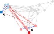
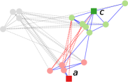
(a) query $S_{1}=\left\{a\right\}$ and $S_{2}=\left\{b\right\}$	(b) query $S_{1}=\left\{a\right\}$ and $S_{2}=\left\{c\right\}$

Figure 1. A motivating example of local polarization search on the New Guinea Highland Tribes graph (Read, 1954): individual tribes are shown as vertices, with friendly relations shown as solid line and enemy relations as dashed line. Given a pair of node sets $(S_{1},S_{2})$ as query, we are interested in finding two subgraphs $C_{1}$ and $C_{2}$ such that: ($i$) $C_{1}$ and $C_{2}$ are antagonistic to each other ($ii$) $C_{1}$ and $C_{2}$ are friendly inside themselves and ($iii$) nodes in $C_{1}$ and $C_{2}$ are related to $S_{1}$ and $S_{2}$. In the figure, we show two querying scenarios. (a) querying $S_{1}=\left\{a\right\}$ and $S_{2}=\left\{b\right\}$ produces $C_{1}$ and $C_{2}$ as the red and blue nodes respectively. (b) querying $S_{1}=\left\{a\right\}$ and $S_{2}=\left\{c\right\}$ produces $C_{1}$ and $C_{2}$ as the red and green nodes. Note that the two pairs of subgraphs are overlapping in red-colored nodes.

1.1. Related work

Local community detection. The problem of finding local communities with respect to seed nodes has been studied extensively. In general, given a set of seed nodes $S$ the task is to find a subgraph that contains $S$ and optimizes some quality measure. Various measures have been proposed, such as conductance (Andersen et al., 2006), $k$-core (Sozio and Gionis, 2010), $k$-truss (Huang et al., 2014), and quasi-cliques (Cui et al., 2014). One line of effort utilizes PageRank methods (Andersen et al., 2006; Gleich and Seshadhri, 2012; Kloster and Gleich, 2014; Bian et al., 2018), which enjoy provable performance guarantee (Andersen et al., 2006) and are effective in practice (Kloumann and Kleinberg, 2014). Mahoney et al. (Mahoney et al., 2012) combine seed information with spectral partitioning and obtain guarantees with respect to conductance.

Our approach is inspired by the work of Mahoney et al. (Mahoney et al., 2012), and our paper extends their results to signed graphs. Yet, to make the extension possible, several technical results are introduced. First, given the spectral properties of signed graphs, we work with $\mathbf{v}_{1}$, the eigenvector of the smallest eigenvalue, while Mahoney’s work use $\mathbf{v}_{2}$, the eigenvector of the second smallest eigenvalue. This key difference leads to a different problem, as the solution is no longer orthogonal to the first vector. In addition, different intermediate results and proofs are required. Second, we rely on recent results on signed graphs (i.e., Proposition 1 in Section 2), not present in the literature on unsigned graphs to the best of our knowledge. Third, efficient rounding of fractional solutions is more complicated on signed graphs than on unsigned graphs, and new techniques are necessary.

Spectral graph theory on signed graphs. Spectral methods have been studied extensively also for signed graphs. Kunegis et al. (Kunegis et al., 2010) study normalized cuts, while Chiang et al. (Chiang et al., 2012) study $k$-way partitioning. Mercado et al. (Mercado et al., 2016) propose the use of the geometric mean of the Laplacians of the positive and negative parts of the graph to correctly cluster graphs under the stochastic block model. Note that all these methods are global, while our method is local.

The spectrum of the signed Laplacian reveals interesting properties about the corresponding graph. The smallest eigenvalue bounds the frustration number (resp. index) (Belardo, 2014; Li and Li, 2009), which is the minimum number of nodes (resp. edges) to remove to make graph balanced. Notably, Atay et al. (Atay and Liu, 2020) shows that the smallest eigenvalue of the normalized Laplacian is closely related to signed bipartiteness ratio, which can be seen as a signed analogue of conductance.

Antagonistic communities. Finding antagonistic communities in signed graphs (Chu et al., 2016; Gao et al., 2016; Lo et al., 2013; Bonchi et al., 2019) has attracted attention in recent years. Existing works differ in the definition of an antagonistic community. Most works focus on enumerating antagonistic communities at the global level, and implicitly reduce information redundancy by avoiding overlapping communities. In contrast, we focus on locating antagonistic communities given seed nodes. It should be noted that our setting is one approach to deal with overlapping structures, e.g., as depicted in Figure 1. Furthermore, our approach yields approximation guarantees in terms of our definition of antagonism, while previous methods employ heuristics without quality guarantees.

2. Problem formulation

We represent column vectors by boldface lower-case letters, e.g., $\mathbf{x},\mathbf{y}$, and matrices by upper-case letters, e.g., $A$, $D$. We write $\mathbf{x}_{i}$ to denote the $i$-th entry in vector $\mathbf{x}$ and $A_{i,j}$ to denote the $j$-th entry in the $i$-th row of matrix $A$. Our notation is shown in Table 1.

Table 1. Notation

Symbol	Meaning
$E^{\text{+}},E^{\text{--}}$	positive/negative edges
$A^{\text{+}},A^{\text{--}},A$	positive/negative/signed adjacency matrix
$D$	degree matrix
$\mathit{vol}(C)$	volume of node set $C$
$L,\mathcal{L}$	unnormalized/normalized signed Laplacian matrix
$\lambda_{1},\mathbf{v}_{1}$	smallest eigenvalue of $\mathcal{L}$ and its eigenvector
$C_{1},C_{2}$	two bands of a polarized community
$S_{1},S_{2}$	seed sets corresponding to the two bands
$\beta(C_{1},C_{2})$	signed bipartiteness ratio of $C_{1},C_{2}$
$k$	volume parameter in LocalPolar-Discrete
$\mathbf{s}$	seed vector in LocalPolar
$\kappa$	correlation parameter in LocalPolar
$h(S_{1},S_{2},k)$	local signed Cheeger’s constant w.r.t $S_{1},S_{2}$ and $k$
$\lambda(\mathbf{s},\kappa)$	locally-biased smallest eigenvalue w.r.t. $\mathbf{s}$ and $\kappa$

Signed graphs. A signed graph is defined as an undirected graph $G=(V,E^{\text{+}},E^{\text{--}})$, where $V=\left\{1,\ldots,n\right\}$ is a set of nodes, $E^{\text{+}}$ a set of positive edges, and $E^{\text{--}}$ a set of negative edges. The set of all edges is $E=E^{\text{+}}\cup E^{\text{--}}$. The adjacency matrix of the positive edges of the graph is denoted by $A^{\text{+}}$. The entry $A^{\text{+}}_{i,j}$ is defined to be 1 (or another positive value if the graph is weighted) if $(i,j)\in E^{\text{+}}$, and 0 otherwise. The adjacency matrix of the negative edges of the graph is denoted by $A^{\text{--}}$ and is defined a similar way. We combine $A^{\text{+}}$ and $A^{\text{--}}$ into a single term, the signed adjacency matrix $A=A^{\text{+}}-A^{\text{--}}$. We focus on undirected graphs, so $A^{\text{+}}$, $A^{\text{--}}$, and $A$ are all symmetric.

Spectral graph theory on signed graphs. Given a signed graph $G=(V,E^{\text{+}},E^{\text{--}})$ we define the following matrices: the degree matrix $D$ is a diagonal matrix with $D_{i,i}=\mathit{deg}(i)=\sum_{j=1}^{n}|A_{i,j}|$; the signed Laplacian matrix is defined as $L=D-A$. Normalizing $L$ gives the signed normalized Laplacian $\mathcal{L}=D^{-\frac{1}{2}}LD^{-\frac{1}{2}}=I-D^{-\frac{1}{2}}AD^{-\frac{1}{2}}$.

Given a vector $\mathbf{x}\in^{n}$ and associated vector $\mathbf{y}=D^{\frac{1}{2}}\mathbf{x}$, we define the Rayleigh quotient $\mathcal{R}_{\mathcal{L}}(\mathbf{y})$:

(1) $$\mathcal{R}_{\mathcal{L}}(\mathbf{y})=\frac{\mathbf{y}^{T}\mathcal{L}\mathbf{y}}{\mathbf{y}^{T}\mathbf{y}}=\frac{\mathbf{x}^{T}L\mathbf{x}}{\mathbf{x}^{T}D\mathbf{x}}.$$

Minimizing $\mathcal{R}_{\mathcal{L}}(\mathbf{y})$ yields the smallest eigenvalue $\lambda_{1}$ of $\mathcal{L}$ and its associated eigenvector $\mathbf{v}_{1}$. If $G$ is connected, a small value of $\lambda_{1}$ indicates a more “balanced” graph, where a graph $G$ is perfectly balanced if its nodes can be partitioned into two sets $C_{1}$ and $C_{2}$, such that all edges within $C_{1}$ and $C_{2}$ are positive and all edges across are negative. If $G$ is perfectly balanced, $\lambda_{1}$ is zero. Otherwise, we say it is unbalanced. The eigenvector $\mathbf{v}_{1}$ gives hints on a node partitioning to minimize $\mathcal{R}_{\mathcal{L}}$.

Measuring polarization. We define a polarized community $(C_{1},C_{2})$ as two disjoint sets of nodes $C_{1},C_{2}\subseteq V$, such that ($i$) there are relatively few (resp. many) negative (resp. positive) edges within $C_{1}$ and within $C_{2}$; ($ii$) there are relatively few (resp. many) positive (resp. negative) edges across $C_{1}$ and $C_{2}$; and ($iii$) there are relatively few edges (of either sign) from $C_{1}$ and $C_{2}$ to the rest of the graph. We refer to $C_{1}$ and $C_{2}$ as the two bands of the community.

Before formalizing the degree of polarization of a community, we introduce some additional notation. Given a set of edges $F$ and two node sets $X,Y\subseteq V$, we consider the edges of $F(X,Y)$ that have one endpoint in $X$ and one in $Y$, i.e., $F(X,Y)=\left\{(u,v)\in F\mid u\in X,v\in Y\right\}$. We define $F(X)=F(X,X)$. For example, $E^{\text{+}}(X)$ is the set of positive edges having both endpoints in $X$. The volume of a node set $S$ is defined as $\mathit{vol}(S)=\sum_{i\in S}\mathit{deg}(i)$.

We also represent a community $(C_{1},C_{2})$ in vector form. Given bands $C_{1}$ and $C_{2}$, we consider a vector $\mathbf{x}\in\left\{-1,0,1\right\}^{n}$ such that $\mathbf{x}_{i}=1$ if $i\in C_{1}$, $\mathbf{x}_{i}=-1$ if $i\in C_{2}$, and $\mathbf{x}_{i}=0$ otherwise.

We now proceed to define our polarization measure: given a community with two bands $(C_{1},C_{2})$ we measure the degree of polarization in the community by

(2) $$\begin{split}\beta(C_{1},C_{2})=\;&\frac{2{\left|E^{\text{+}}(C_{1},C_{2})\right|}+{\left|E^{\text{--}}(C_{1})\right|}+{\left|E^{\text{--}}(C_{2})\right|}}{\mathit{vol}(C_{1}\cup C_{2})}\\ &+\frac{{\left|E(C_{1}\cup C_{2},V\setminus(C_{1}\cup C_{2}))\right|}}{\mathit{vol}(C_{1}\cup C_{2})}.\end{split}$$

We refer to the quantity $\beta$ as signed bipartiteness ratio (Atay and Liu, 2020). In particular, the more polarized the community $(C_{1},C_{2})$ the smaller the value of $\beta(C_{1},C_{2})$. Using $\mathbf{x}$ (defined over $C_{1},C_{2}$) and $\mathbf{y}=D^{\frac{1}{2}}\mathbf{x}$, the following relation holds:

(3) $$\begin{split}\mathcal{R}_{\mathcal{L}}(\mathbf{y})=\;&\frac{\mathbf{x}^{T}L\mathbf{x}}{\mathbf{x}^{T}D\mathbf{x}}\\ =\;&\frac{4{\left|E^{\text{+}}(C_{1},C_{2})\right|}+4{\left|E^{\text{--}}(C_{1})\right|}+4{\left|E^{\text{--}}(C_{2})\right|}}{\mathit{vol}(C_{1}\cup C_{2})}\\ &+\frac{{\left|E(C_{1}\cup C_{2},V\setminus(C_{1}\cup C_{2}))\right|}}{\mathit{vol}(C_{1}\cup C_{2})}.\end{split}$$

Note that $\mathcal{R}_{\mathcal{L}}(\mathbf{y})$ and $\beta(C_{1},C_{2})$ bound each other by a constant factor:

(4) $$\beta(C_{1},C_{2})\leq\mathcal{R}_{\mathcal{L}}(\mathbf{y})\leq 4\beta(C_{1},C_{2}).$$

Intuitively, minimizing $\beta(C_{1},C_{2})$ is closely related to minimizing the corresponding $\mathcal{R}_{\mathcal{L}}(\mathbf{y})$.

As in the work of Atay and Liu (Atay and Liu, 2020), we refer to

$$h(G)=\min_{C_{1},C_{2}}\beta(C_{1},C_{2})$$

as the signed Cheeger constant of the graph $G$.

Encoding information about seed nodes. In this paper we consider a setting where a set of seed nodes is given as input. We sometimes refer to seeds as query nodes. The seed nodes are specified as two disjoint sets $(S_{1},S_{2})$, i.e., $S_{1},S_{2}\subseteq V$ and $S_{1}\cap S_{2}=\varnothing$. The sets $S_{1}$ and $S_{2}$ are meant to provide example nodes for the two bands of the polarized community we are interested in discovering. Typically, ${\left|S_{1}\right|}$ and ${\left|S_{2}\right|}$ are small.

Intuitively, we are seeking a community $(C_{1},C_{2})$ such that each band contains one of the seed sets, e.g., $S_{1}\subseteq C_{1}$ and $S_{2}\subseteq C_{2}$ and at the same time minimizes $\beta(C_{1},C_{2})$. In addition, we are interested in solutions whose size is bounded with respect to the size of the seed nodes and are preferably well connected to these. We express this as a constraint of the volume of the set $C_{1}\cup C_{2}$ normalized by the volume of the set $S_{1}\cup S_{2}$. In particular, we require that the volume of the solution $\mathit{vol}(C_{1}\cup C_{2})$ is at most $k$ times the volume of the seed nodes $\mathit{vol}(S_{1}\cup S_{2})$, where $k$ is a user-defined parameter. We formalize this problem as follows:

Problem 0 (LocalPolar-Discrete).

Given a signed graph $G$, a pair of seed sets $(S_{1},S_{2})$ and a positive number $k\in^{+}$ our goal is to find a polarized community $(C_{1},C_{2})$ so that

1. $(C_{1},C_{2})$ minimizes the signed bipartiteness ratio $\beta(C_{1},C_{2})$;

2. $S_{1}\subseteq C_{1}\text{ and }S_{2}\subseteq C_{2}$;

3. $\frac{\mathit{vol}(C_{1}\cup C_{2})}{\mathit{vol}(S_{1}\cup S_{2})}\leq k$;

Adapting the notion of signed Cheeger’s constant $h(G)$, we define a local variant of $h(G)$. Given a signed graph $G$, two disjoint node sets $S_{1}$ and $S_{2}$, and a positive number $k$, local signed Cheeger’s constant is defined as:

(5) $$h(S_{1},S_{2},k)=\!\!\!\!\!\!\!\!\min_{\begin{subarray}{c}C_{1},C_{2}\subseteq V:\\ S_{1}\subseteq C_{1},S_{2}\subseteq C_{2}\\ \mathit{vol}({C_{1}\cup C_{2}})/\mathit{vol}(S_{1}\cup S_{2})\leq k\end{subarray}}\!\!\!\!\!\!\!\!\beta(C_{1},C_{2})$$

Next, we consider a continuous variant of the LocalPolar-Discrete problem. The theoretical properties of the continuous problem will be studied soon. First, let $\mathbf{x}$ be continuous, i.e., $\mathbf{x}\in^{n}$. Second, we encode the query information via a seed vector $\mathbf{s}\in^{n}$. Seed nodes take non-zero values in $\mathbf{s}$ and signs indicate membership in $S_{1}$, or $S_{2}$: by convention, $\mathbf{s}_{i}>0$ if $i\in S_{1}$, $\mathbf{s}_{i}<0$ if $i\in S_{2}$, and $\mathbf{s}_{i}=0$ otherwise. The magnitude of the coordinate $\mathbf{s}_{i}$ indicates the strength by which we require that the solution contains the node $i$. A special case of our setting is when one of the two query sets is empty, i.e., $S_{1}=\varnothing$ or $S_{2}=\varnothing$. For technical reasons, we normalize $\mathbf{s}$ with respect to node degree, e.g., $\mathbf{s}^{T}D\mathbf{s}=1$.

We formalize the continuous problem below.

Problem 0 (LocalPolar).

Given a signed graph $G$, a seed vector $\mathbf{s}\in^{n}$, and a correlation parameter $\kappa$, our goal is to find a vector $\mathbf{x}\in^{n}$ such that

(6) $$\underset{\mathbf{x}}{\text{minimize}} \mathbf{x}^{T}L\mathbf{x}$$

such that $$\mathbf{x}^{T}D\mathbf{x}=1$$

$$\mathbf{x}^{T}D\mathbf{s}\geq\kappa$$

$$\mathbf{x}\in^{n}.$$

The parameter $\kappa$ controls the correlation between $\mathbf{x}$ and $\mathbf{s}$. Notice that LocalPolar is not convex due to the constraint $\mathbf{x}^{T}D\mathbf{x}=1$.

It can be shown that LocalPolar is indeed a continuous relaxation of LocalPolar-Discrete. This is shown in Claim 1, below. Using this result, we can solve an instance of the LocalPolar-Discrete problem, by first solving its continuous relaxation and then rounding the solution to a discrete one. The result is also used to prove the approximation guarantee for LocalPolar-Discrete.

Before stating the claim, we introduce some additional notation. For $S\subseteq V$, we let $1_{S}\in\left\{0,1\right\}^{n}$ be a vector that has 1 at entries in $S$ and 0 otherwise. Then, for two disjoint sets $A,B\subseteq V$, we define the vector $\mathbf{s}_{A,B}=(1_{A}-1_{B})/\sqrt{\mathit{vol}(A\cup B)}$. It can be checked that $\mathbf{s}_{A,B}^{T}\;D\;\mathbf{s}_{A,B}=1$.

Claim 1.

For any $S_{1},S_{2}\subseteq V$, LocalPolar($G,\mathbf{s}_{S_{1},S_{2}},\sqrt{1/k}$) is a relaxation of LocalPolarDiscrete($G,S_{1},S_{2},k$). In particular,

(7) $$\lambda(\mathbf{s}_{S_{1},S_{2}},\sqrt{1/k})\leq 4h(S_{1},S_{2},k),$$

where $\lambda(\mathbf{s}_{S_{1},S_{2}},\sqrt{1/k})$ is the optimal value of LocalPolar($G,\mathbf{s}_{S_{1},S_{2}},\sqrt{1/k}$) and $h(S_{1},S_{2},k)$ is the optimal value of LocalPolarDiscrete($G,S_{1},S_{2},k$).

Proof.

First, the objective of LocalPolar relaxes the objective of LocalPolar-Discrete because LocalPolar optimizes over a continuous space and the two objectives bound each other up to constant factors (Equation 4).

Second, LocalPolar relaxes both constraints of LocalPolar-Discrete and translates them into the correlation constraint. Consider any feasible solution $C_{1}$ and $C_{2}$ of LocalPolar-Discrete, and let $C=C_{1}\cup C_{2}$ and $S=S_{1}\cup S_{2}$. Also let $\mathbf{x}=\mathbf{s}_{C_{1},C_{2}}$ and $\mathbf{s}=\mathbf{s}_{S_{1},S_{2}}$ to be used in LocalPolar. Expanding $\mathbf{x}^{T}D\mathbf{s}$ gives:

$$\mathbf{x}^{T}D\mathbf{s} =\frac{1}{\sqrt{\mathit{vol}(C)\mathit{vol}(S)}}(1_{C_{1}}-1_{C_{2}})^{T}D(1_{S_{1}}-1_{S_{2}})$$

$$=\frac{1}{\sqrt{\mathit{vol}(C)\mathit{vol}(S)}}(1_{C_{1}}^{T}D1_{S_{1}}+1_{C_{2}}^{T}D1_{S_{2}})$$

$$=\frac{1}{\sqrt{\mathit{vol}(C)\mathit{vol}(S)}}(\mathit{vol}(S_{1})+\mathit{vol}(S_{2}))$$

$$=\sqrt{\frac{\mathit{vol}(S)}{\mathit{vol}(C)}}\geq\sqrt{\frac{1}{k}}.$$

Line 2 follows from: $C_{1}\cap C_{2}=\varnothing$, $S_{1}\cap S_{2}=\varnothing$ and $S_{1}\subseteq C_{1},S_{2}\subseteq C_{2}$.

Last, it is easy to verify $\mathbf{x}^{T}L\mathbf{x}\leq 4\beta(C_{1},C_{2})$. Also by definition, we have $\lambda(\mathbf{s}_{S_{1},S_{2}},\sqrt{1/k})\leq\mathbf{x}^{T}L\mathbf{x}$. So it follows immediately that $\lambda(\mathbf{s}_{S_{1},S_{2}},\sqrt{1/k})\leq 4h(S_{1},S_{2},k)$. ∎

In the next section, we analyze the properties of LocalPolar and propose an approximation algorithm for LocalPolar-Discrete.

3. Theoretical analysis

We first present how to solve the continuous problem LocalPolar and obtain an optimal solution $\mathbf{x}^{*}$. This is stated in Theorem 1. Then, we describe how to round the continuous optimal solution $\mathbf{x}^{*}$ so as to obtain a discrete solution to LocalPolar-Discrete with approximation ratio $\mathcal{O}(\sqrt{h(S_{1},S_{2},k)})$. Finally, we present an efficient algorithm PolarSeeds (Algorithm 1) that leverages these results.

Theorem 1 (Solution characterization).

Given an unbalanced signed graph $G$ with normalized Laplacian matrix $\mathcal{L}$, let $\mathbf{s}\in^{n}$ be a seed vector, with $\mathbf{s}^{T}D\mathbf{s}=1$ and $\mathbf{s}^{T}D\mathbf{v}_{1}\neq 0$, where $\mathbf{v}_{1}$ is the eigenvector of the smallest eigenvalue of $\mathcal{L}$. Let $0\leq\kappa<1$ be a correlation parameter, and let $\mathbf{x}^{*}$ be an optimal solution to LocalPolar($G,\mathbf{s},\kappa$). Then, there exists some $\alpha\in(-\infty,\lambda_{1})$ and a $\beta\in[0,\infty]$ such that

$$\mathbf{x}^{*}=\beta{(L-\alpha D)}^{\dagger}D\mathbf{s}$$

where ${(L-\alpha D)}^{\dagger}$ is the pseudo inverse of $L-\alpha D$.

Theorem 2 (Approximation guarantee).

Given an unbalanced signed graph $G$, two disjoint node sets $S_{1},S_{2}\in V$, and a positive integer $k$, we can find two disjoint sets $C_{1}$ and $C_{2}$ that achieve $\beta(C_{1},C_{2})=\mathcal{O}(\sqrt{h(S_{1},S_{2},k)})$ from the optimal solution of LocalPolar($G,\mathbf{s}_{S_{1},S_{2}},\sqrt{1/k}$).

We illustrate the high-level structure of our proof in Figure 2.

Figure 2. High-level structure of our proof.

3.1. Proof of Theorem 1

We first relax LocalPolar($G,\mathbf{s},\kappa$) to a convex semi-definite program SDP_p($G,\mathbf{s},\kappa$) shown in Figure 3. Then we show that the optimality gap between SDP_p and LocalPolar is zero. By using the complementary slackness conditions of SDP_p and its dual we show that the solution of SDP_p has rank 1, which characterizes its form. Our proof technique is adapted from Mahoney et al. (Mahoney et al., 2012).

Primal SDPp($G,\mathbf{s},\kappa$)	Dual SDPd($G,\mathbf{s},\kappa$)
$\begin{aligned} &\min_{X}&&L\circ X\\ &\textrm{s.t.}&&D\circ X=1\\ &&&(D\mathbf{s})(D\mathbf{s})^{T}\circ X\geq\kappa\\ &&&X\succeq 0\end{aligned}$	$\begin{aligned} &\max_{\alpha,\beta}&&\alpha+\beta\kappa\\ &\textrm{s.t.}&&L\succeq\alpha D+\beta(D\mathbf{s})(D\mathbf{s})^{T}\\ &&&\beta\geq 0\\ &&&\alpha\in\end{aligned}$

Figure 3. SDP relaxation of LocalPolar($G,\mathbf{s},\kappa$) (left) and its dual problem (right)

To see that SDP_p is a relaxation of LocalPolar, consider a feasible solution $x$ of LocalPolar. Then $X=xx^{T}$ is also a feasible solution for SDP_p and $X\circ L=\mathbf{x}^{T}L\mathbf{x}$.

The following two claims are based on known results in convex optimization (Boyd and Vandenberghe, 2004):

Claim 2.

Strong duality holds between SDP_p($G,\mathbf{s},\kappa$) and SDP_d($G,\mathbf{s},\kappa$).

Proof.

As SDP_p($G,\mathbf{s},\kappa$) is a convex problem, Slater’s condition is sufficient to verify zero duality gap (Boyd and Vandenberghe, 2004) (Chapter 5.5.3). By setting $X=\mathbf{s}\mathbf{s}^{T}$, we have $(D\mathbf{s})(D\mathbf{s})^{T}\circ\mathbf{s}\mathbf{s}^{T}=(\mathbf{s}^{T}D\mathbf{s})^{2}=1>\kappa$, i.e., strong feasibility holds. Therefore Slater’s condition is satisfied. ∎

Claim 3.

Strong duality holds between SDP_p($G,\mathbf{s},\kappa$) and SDP_d($G,\mathbf{s},\kappa$). Therefore, the feasibility and complementary slackness conditions suffice to establish optimality.

The feasibility conditions are:

(8) $$D\circ X^{*} =1,$$

$$(D\mathbf{s})(D\mathbf{s})^{T}\circ X^{*} \geq\kappa,$$

$$X^{*} \succeq 0$$

(9) $$L-\alpha^{*}D-\beta^{*}(D\mathbf{s})(D\mathbf{s})^{T} \succeq 0,\>and$$

$$\beta^{*} \geq 0$$

and complementary slackness conditions are:

(10) $$\beta^{*}((D\mathbf{s})(D\mathbf{s})^{T}\circ X^{*}-\kappa) =0,\>and$$

(11) $$X^{*}\circ(L-\alpha^{*}D-\beta^{*}(D\mathbf{s})(D\mathbf{s})^{T}) =0$$

Proof.

These conditions directly follow from the optimality conditions of semi-definite programs (Boyd and Vandenberghe, 2004) (Chapter 5.9.2). ∎

A key finding is the following claim. The proof is given in the Appendix.

Claim 4.

The rank of $X^{*}$ is 1, i.e, $X^{*}=\mathbf{x}^{*}(\mathbf{x}^{*})^{T}$, and therefore the optimality gap between LocalPolar($G,\mathbf{s},\kappa$) and SDP_p($G,\mathbf{s},\kappa$) is 0.

Claim 5.

Given that $X^{*}$ has the form $\mathbf{x}^{*}(\mathbf{x}^{*})^{T}$, the feasibility and complementary slackness conditions imply,

$$\mathbf{x}^{*}=\pm\beta^{*}\sqrt{\kappa}{(L-\alpha^{*}D)}^{\dagger}D\mathbf{s}.$$

Proof.

Using Claim 4, we have $X^{*}=\mathbf{x}^{*}(\mathbf{x}^{*})^{T}$. Relying on equation (9) we can rewrite Equation (11) as:

$$(L-\alpha^{*}D-\beta^{*}(D\mathbf{s})(D\mathbf{s})^{T})\mathbf{x}^{*} =0$$

$$(L-\alpha^{*}D)\mathbf{x}^{*} =\pm\beta^{*}\sqrt{\kappa}D\mathbf{s}$$

$$\mathbf{x}^{*} =\pm\beta^{*}\sqrt{\kappa}{(L-\alpha^{*}D)}^{\dagger}D\mathbf{s}.$$

The 2nd line follows from Equation (10), as $(D\mathbf{s})^{T}\mathbf{x}^{*}=\pm\sqrt{\kappa}$. ∎

3.2. Proof of Theorem 2

Our proof relies on Cheeger’s inequality for signed graphs:

Proposition 0.

(Lemma 4.2 by Atay et al. (Atay and Liu, 2020)) For any non-zero vector $\mathbf{x}\in^{{\left|V\right|}}$, there exists a $t\in[0,\max_{u\in V}{\left|\mathbf{x}_{u}\right|}]$ such that

$$\beta(V_{\mathbf{x}}(t),V_{\mathbf{x}}(-t))\leq\sqrt{2\frac{\mathbf{x}^{T}L\mathbf{x}}{\mathbf{x}^{T}D\mathbf{x}}}$$

where $V_{\mathbf{x}}(t)=\left\{u\in V\mid\mathbf{x}_{u}\geq t\right\}\text{ and }V_{\mathbf{x}}(-t)=\left\{u\in V\mid\mathbf{x}_{u}\leq-t\right\}$.

Proof of Theorem 2.

Given a problem instance of LocalPolar with parameters $\mathbf{s}_{S_{1},S_{2}}$ and $\kappa=\sqrt{1/k}$, we apply Theorem 1 and get the optimal vector $\mathbf{x}^{*}$. By Proposition 3, we can get two sets $C_{1}$ and $C_{2}$ that have $\beta(C_{1},C_{2})\leq\sqrt{2\lambda(\mathbf{s}_{S_{1},S_{2}},\sqrt{1/k})}$. Finally, by Claim 1, $\beta(C_{1},C_{2})=\mathcal{O}(\sqrt{h(C_{1},C_{2},k)})$.

3.3. PolarSeeds algorithm

We now summarize the complete algorithm, which we call PolarSeeds. Pseudocode is presented as Algorithm 1. The PolarSeeds algorithm consists of 2 steps: ($i$) approximate within small error the optimal solution $\mathbf{x}^{*}$ of the problem SDP_p, using Theorem 1; and ($ii$) round $\mathbf{x}^{*}$ to obtain an integral solution, using Proposition 3. We discuss these two steps in more detail.

Data: Signed graph $G=(V,E^{\text{+}},E^{\text{--}})$, seeds $(S_{1},S_{2})$, $k\in^{+}$ and tolerance parameter $\epsilon>0$

Result: two bands $(C_{1},C_{2})$

1 Create seed vector $\mathbf{s}$ s.t. $\mathbf{s}_{i}=1\text{ if }i\in C_{1}$ and $\mathbf{s}_{i}=-1\text{ if }i\in C_{2}$;

2 normalize $\mathbf{s}$ s.t. $\mathbf{s}^{T}D\mathbf{s}=1$;

3 $\kappa=1/\sqrt{k},\ \ell\leftarrow-\mathit{vol}(V),\ u\leftarrow\lambda_{1}$;

4 repeat

5       $\alpha\leftarrow(\ell+u)/2$;

6       Solve $(L-\alpha D)\mathbf{x}=D\mathbf{s}$ using Conjugate Gradient method;

7       normalize $\mathbf{x}$ s.t. $\mathbf{x}^{T}D\mathbf{x}=1$;

8       if $\sqrt{\kappa}-\mathbf{s}^{T}D\mathbf{x}<0$ then $\ell\leftarrow\alpha$;

9      else $u\leftarrow\alpha$;

10      

11until $-\epsilon\leq\sqrt{\kappa}-\mathbf{s}^{T}D\mathbf{x}\leq 0$;

12 Find $t\in^{+}$ that minimizes $\beta(V_{\mathbf{x}}(t),V_{\mathbf{x}}(-t))$;

return $(V_{\mathbf{x}}(t),V_{\mathbf{x}}(-t))$

Algorithm 1 PolarSeeds. The algorithm first approximates $\mathbf{x}^{*}$ by performing binary search on $\alpha$ (lines 1–1). Then, $(C_{1},C_{2})$ is attained by rounding $\mathbf{x}$ at line 1. An $\mathcal{O}(m+n\log n)$ rounding procedure is described in Appendix A.2.

Computing the optimal solution $\mathbf{x}^{*}$. We discuss how to find the optimal solution $\mathbf{x}^{*}=\beta^{*}{(L-\alpha^{*}D)}^{\dagger}D\mathbf{s}$ without knowing the value of $\alpha^{*}$ beforehand. If we assume that $\alpha^{*}$ is known, then ${(L-\alpha^{*}D)}^{\dagger}$ can be approximated using Conjugate Gradient Method (Golub and Van Loan, 2012) in time $\mathcal{O}({m\sqrt{c}})$, where $c$ is the condition number of $L-\alpha^{*}D$.

Then, to approximate $\alpha^{*}$, we use complementary slackness condition Equation (10) and apply binary search on $\alpha\in[-\mathit{vol}(G),\lambda_{1})$. The search stops when $\mathbf{x}^{T}(D\mathbf{s})(D\mathbf{s})^{T}\mathbf{x}$ is close enough to $\kappa$ (controlled by $\epsilon$). The whole process requires time $\mathcal{O}(\sqrt{c}m\log(m))$.

Lines 1 to 1 in Algorithm 1 describe the above process.

Rounding $\mathbf{x}^{*}$. We want to find a value $t\in^{+}$ that minimizes $\beta(V_{\mathbf{x}}(t),V_{\mathbf{x}}(-t))$. A naïve way is to try each value in $\mathbf{x}$ for $t$, compute the corresponding $\beta(V_{\mathbf{x}}(t),V_{\mathbf{x}}(-t))$ from scratch (doable in time $\mathcal{O}(m)$) and take the value of $t$ that minimizes $\beta$. The total runtime cost is $\mathcal{O}(mn+n\log(n))$.

We propose a faster procedure, which incrementally computes $\beta(V_{\mathbf{x}}(t),V_{\mathbf{x}}(-t))$ for values of $t$ in ascending order. The time cost reduces to $\mathcal{O}(m+n\log(n))$. Moreover, our implementation leverages basic vector and matrix operations, which further boost speed in practice. The details are described in Appendix A.2.

4. Experimental evaluation

In this section we evaluate the performance of the proposed algorithm. Our experimental evaluation is structured as follows. First in Section 4.1, we experiment with synthetic graphs to better understand the behavior of our method under different scenarios. In Section 4.2, we compare with a state-of-the-art method (Chu et al., 2016) for polarized community detection on real-world graphs. In Section 4.3 we discuss two case studies, and finally, in Section 4.4 we demonstrate the scalability of our algorithm.

We implement our algorithm in Python and perform the experiment on a Linux machine with a 10-core CPU and 64 GB of memory. We use the Conjugate Gradient solver implemented in Scipy 1.2.1 with the default parameters. We set the binary search parameter $\epsilon=10^{-3}$ (used by Algorithm 1).

The implementation of the code will be available in the non-anonymized version of the paper.

Table 2. Real-word signed graphs: $\lambda_{1}$ is the smallest eigenvalue of the normalized Laplacian.

Signed graph	${\left|V\right|}$	${\left|E\right|}$	${\left|E^{\text{--}}\right|}/{\left|E\right|}$	$\lambda_{1}$	Category
Word	5 K	47 K	0.20	0.030	language
Bitcoin	6 K	21 K	0.15	0.040	social
Referendum	11 K	251 K	0.05	0.039	political
Slashdot	82 K	500 K	0.24	0.017	social
Epinions	119 K	704 K	0.17	0.011	social
WikiConflict	113 K	2 000 K	0.63	0.075	edit conflict
WikiConflict-1M	1 M	33 M	0.63	0.075	artificial

Real-world datasets. We choose publicly-available real-world signed graphs, whose statistics are summarized in Table 2. Word (Sedoc et al., 2018) captures the synonym-and-antonym relation among words in the English language. A synonym (resp. antonym) pair is connected by an edge with positive (resp. negative) weight, where a weight represents the strength of similarity (resp. opposition). Referendum (Lai et al., 2018) records the 2016 Italian Referendum on Twitter: an edge is negative if two users are classified with different stances, and positive otherwise. Bitcoin is a trust network of Bitcoin users. Slashdot is a social network from a technology-news website, which contains friend or foe links among its users. Epinions is a trust online social network from a consumer review site, where site members can decide to trust, or distrust, each other. Edges in WikiConflict represents positive and negative edit conflicts between users on Wikipedia.

To evaluate the scalability of our method, we artificially augment WikiConflict to WikiConflict-1M. The procedure is described in Section 4.4. We experiment with the largest weakly-connected component of each graph. Directed graphs are converted to undirected ones with adjacency matrix $(A+A^{T})/2$.

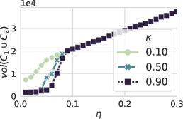
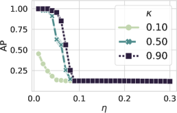
(a)	(b)	(c)
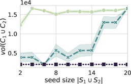
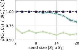
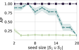
(d)	(e)	(f)

Figure 4. Performance of different metrics on synthetic graphs. 1st/2nd/3rd columns corresponds to : solution volume / $\beta$ ratio / average precision respectively. Meanwhile, we vary 2 parameters: (i) edge noise parameter $\eta$ (top row); (ii) seed size $q$ for $C_{1}^{*}$ and $C_{2}^{*}$ (bottom row). Results are shown for 3 values of the parameter $\kappa$. In figure (b), we use a red solid line at $y=1$ to differentiate two cases of $\beta$ ratio. Error bars at 0.95 confidence interval is drawn in the form of shaded area.

Synthetic datasets. To better assess the effectiveness of our method under different scenarios, we create random graphs containing 8 ground-truth polarized communities, $\left\{(C_{i,1},C_{i,2})\mid i=1,\dots,8\right\}$. For simplicity, we assume that all bands are of the same size, $20$. In addition, the creation process is controlled by an edge-noise parameter $\eta\in[0,1]$, where large values of $\eta$ indicate more noise in edge signs. The role of edge-noise parameter $\eta$ is as follows:

• for each pair of nodes within $C_{i,1}$ or $C_{i,2}$, for $i=1,\ldots,p$, there is a positive edge with probability $1-\eta$, a negative edge with probability $\eta/2$, and non edge with probability $\eta/2$;

• for each pair of nodes, one in $C_{i,1}$ and the other in $C_{i,2}$, for $i=1,\ldots,p$, there is a negative edge with probability $1-\eta$, a positive edge with probability $\eta/2$, and a non edge with probability $\eta/2$;

• for every other pair of nodes in the graph there is a non edge with probability $1-\eta$, a positive edge with probability $\eta/2$, and a negative edge with probability $\eta/2$.

In our experiments, we also vary the size of seed set ${\left|S_{1}\cup S_{2}\right|}$ and the value of $\kappa$. For simplicity, we make ${\left|S_{1}\right|}={\left|S_{2}\right|}$.

Baseline. We compare our method with a state-of-the-art method on discovering polarized communities on real-world graphs. The focg algorithm (Chu et al., 2016) is designed to discover $k$-way polarized communities. Note that focg is a global method, and thus, not directly comparable with our approach; we select focg as baseline as it is the most related work in the literature. focg returns a set of $k$-way polarized communities, $\left\{\mathcal{C}_{i}\right\}_{i=1}^{\ell}$, where $\mathcal{C}_{i}=(C_{i1},\ldots,C_{ik})$ and $\ell$ is determined by the algorithm. focg ensures that $\mathcal{C}_{i}\cap\mathcal{C}_{j}=\varnothing$ for all $i\neq j$. We use $k=2$ and set the other parameters as suggested. We exclude communities that either ($i$) are too small, in particular, ${\left|C_{1}\right|}\text{ or }{\left|C_{2}\right|}\leq 5$, or ($ii$) the two bands intersect.

4.1. Evaluation on synthetic graphs

By studying the effects of various parameters including algorithm and graph generation parameters, we aim to answer the following research questions:

• Q1: what is the effect of parameter $\kappa$ on the characteristics of the solution, as well as in the accuracy of finding the ground truth?

• Q2: what is the effect of noise in the behavior of PolarSeeds?

• Q3: can we find a polarized community more accurately by giving more seeds to PolarSeeds?

We report the average performance for each configuration over a combination of 10 randomly generated graphs and 10 randomly selected ground-truth communities paired with random seeds in them.

Evaluation metric. Given a solution $(C_{1},C_{2})$ and ground truth $(C_{1}^{*},C_{2}^{*})$, we measure its average precision.

$$\text{\sc\large ap}(C_{1},C_{2})=\frac{1}{2}\left(\frac{{\left|C_{1}\cap C_{1}^{*}\right|}}{{\left|C_{1}\right|}}+\frac{{\left|C_{2}\cap C_{2}^{*}\right|}}{{\left|C_{2}\right|}}\right).$$

We also report the ratio $\beta(C_{1},C_{2})/\beta(C_{1}^{*},C_{2}^{*})$, referred as $\beta$-ratio for brevity. The motivation is to see whether our method can find a solution that is even better than the ground truth, according to the optimized measure, which happens when $\beta$ ratio $<1$. Finally, we report the solution volume $\mathit{vol}(C_{1}\cup C_{2})$.

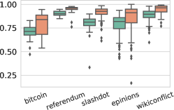
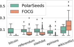
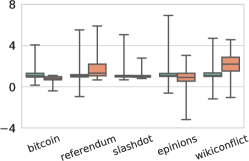
(a) Signed Bipartiteness Ratio $\beta$	(b) ham	(c) $\log_{2}(\text{$\text{Polarity}$})$

Figure 5. Distributions of 3 evaluation metrics on all communities found by PolarSeeds and focg. focg returns multiple communities by design. We randomly seed PolarSeeds multiple rounds in order to find multiple communities. Overlapping communities are filtered out to make the comparison fair. For $\beta$, smaller values indicates better performance, while for ham and Polarity, larger values are better.

We make the following observations:

Effect of correlation parameter $\kappa$. As a part of the answer to Q1, Figures 4(a) and (d) indicate that smaller $\kappa$ produces solutions with larger $\mathit{vol}(C_{1}\cup C_{2})$. This phenomenon can be explained by Claim 1. Recall that $\kappa=\sqrt{1/k}$, where $k$ upper bounds the solution volume in LocalPolar-Discrete and $\kappa$ is the correlation parameter in LocalPolar. A smaller $\kappa$ implies a larger $k$. Thus, the constraint $\mathit{vol}(C_{1}\cup C_{2})\leq k\mathit{vol}(S_{1}\cup S_{2})$ in LocalPolar-Discrete encourages solutions with larger $\mathit{vol}(C_{1}\cup C_{2})$ if a larger $k$ is given,

With respect to the second part of the question Q1, we observe that larger values of $\kappa$ make PolarSeeds more noise-resistant. Figure 4(c) shows directly that $\kappa=0.9$ achieves the best ap scores. Internally, large $\kappa$ values make PolarSeeds select solutions with small volume, which increases ap scores. This concludes the answer to Q1.

Effect of noise. In Figures 4(a), (b), and (c), we vary $\eta$ from $0.01$ to $0.3$ and set seed size equal to 2, i.e., ${\left|S_{1}\right|}={\left|S_{2}\right|}=1$). Thus, with respect to our research question Q2, we observe that as we increase $\eta$, PolarSeeds is more likely to pick some $C_{1},C_{2}$ other than $C_{1}^{*},C_{2}^{*}$, thus, lowering the ap scores. We explain this phenomenon next.

First, PolarSeeds misses $C_{1}^{*},C_{2}^{*}$ when there is another $C_{1},C_{2}$ that gives better $\beta$, i.e., $\beta(C_{1},C_{2})<\beta(C_{1}^{*},C_{2}^{*})$. This happens when $\eta$ is large enough (shown in Figure 4(b)). On one hand, as we add more noise, $C_{1}^{*},C_{2}^{*}$ becomes less polarized i.e., $\beta(C_{1}^{*},C_{2}^{*})$ increases. When there is a sufficiently large amount of noise, the polarization structure is destroyed, i.e., $\beta(C_{1}^{*},C_{2}^{*})\approx 1$. On the other hand, as $\beta(C_{1}^{*},C_{2}^{*})$ approaches $1$, solutions with larger $\mathit{vol}(C_{1},C_{2})$ are preferred as it makes $\beta(C_{1},C_{2})$ smaller. This is shown by the increased solution volume in Figure 4(a). Combining the above observations, it follows that when the noise increases, the accuracy of PolarSeeds finding $C_{1}^{*},C_{2}^{*}$ decreases.

Effect of seed size. In Figures 4(d), (e), and (f), we vary the seed size on $C_{1}^{*}$ and $C_{2}^{*}$ from 2 to 20 and we set edge noise $\eta=0.05$.

We notice that the effects on all 3 metrics are limited when $\kappa$ is either too large (e.g., $0.9$) or too small (e.g., $0.1$). In contrast, when $\kappa=0.5$, seed size starts to play a remarkable role. For example, as ${\left|S_{1}\cup S_{2}\right|}$ (which is positively correlated with $\mathit{vol}(S_{1}\cup S_{2})$) increases, the solution volume tends to increase (Figure 4(d)). This can be explained by using an argument similar to the effect of $\kappa$ on solution volume, i.e., when $k$ is fixed, larger $\mathit{vol}(S_{1}\cup S_{2})$ allows $\mathit{vol}(C_{1}\cup C_{2})$ to increase. As a consequence, this brings down the ratio $\beta(C_{1},C_{2})/\beta(C_{1}^{*},C_{2}^{*})$ (Figure 4(e)), which further decreases ap scores (Figure 4(f)).

So with respect to question Q3, we conclude that adding more seeds does not necessarily improve the ap score. The value of $\kappa$ affects how much influence the seed number can exert. The influence is limited when $\kappa$ is either too large or too small. On the other hand, when $\kappa$ lies in between, more seeds encourage PolarSeeds to produce larger-volume solutions, reducing ap scores.

4.2. Evaluation on real-world graphs

Next, we compare PolarSeeds with focg and evaluate their capability to finding high-quality polarized communities in real-world graphs. Since focg is “query-less” and tries to enumerate polarized communities, we make the following adaptation to make them comparable. We randomly seed PolarSeeds over multiple rounds and collect the results. As PolarSeeds can produce communities that overlap, for fairness, we keep only one of the overlapping communities . We set $\kappa=0.9$ as we observe that this choice is effective on a wide range of real-world graphs. In addition, $\kappa=0.9$ ensures that the seed nodes have dominant magnitude in the solution, i.e., ${\left|\mathbf{x}^{*}_{s}\right|}$ dominates at $s\in S_{1}\cup S_{2}$.

Evaluation metrics. We use 3 metrics to measure quality:

• Signed bipartiteness ratio $\beta$, the objective of our problem;

• ham, the harmonic mean of Cohesion and Opposition measures, defined by Chu et al. (Chu et al., 2016). In particular,

  $$\text{Cohesion}(C_{1},C_{2}) =\frac{1}{2}[d^{\text{+}}(C_{1})+d^{\text{+}}(C_{2})]$$

  $$\text{Opposition}(C_{1},C_{2}) =d^{\text{--}}(C_{1},C_{2})$$

  with $d^{\text{+}}(C)=\frac{2{\left|E^{\text{+}}(C)\right|}}{{\left|C\right|}({\left|C\right|}-1)}$ and $d^{\text{--}}(C_{1},C_{2})=\frac{{\left|E^{\text{--}}(C_{1},C_{2})\right|}}{{\left|C_{1}\right|}{\left|C_{2}\right|}}$;

• Polarity (Bonchi et al., 2019), which counts the number of edges that agree with the polarized structure and penalizes large communities:

  $$\text{Polarity}(C_{1},C_{2})=\frac{{\left|E^{\text{+}}(C_{1})\cup E^{\text{+}}(C_{2})\right|}+2{\left|E^{\text{--}}(C_{1},C_{2})\right|}}{{\left|C_{1}\cup C_{2}\right|}}.$$

Results. The distributions of the 3 evaluation metrics for both methods are shown in Figure 5. In Figure 5(a), PolarSeeds always outperforms focg w.r.t. the median of $\beta$, which is expected because PolarSeeds optimizes $\beta$. In terms of ham (Figure 5(b)), our method achieves better median value on 4 out of the 5 graphs (except WikiConflict). This result is somehow surprising because focg optimizes an objective closer to ham than our approach. Last in Figure 5(c), there is no clear winner for the Polarity metric.

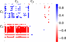
(a) fair as without cheating	(b) fair as not excessive	(c) unilateral distrust in Bitcoin.
e.g., a fair game	e.g., fair amount of time	adjacency matrix of $(C_{1},C_{2})$ is shown

Figure 6. (a) and (b): overlapping communities centered on fair in the Word graph. Seed nodes are: (a) $S_{1}=\left\{\text{{fair}, {honest}}\right\},S_{2}=\left\{\text{{cheating}}\right\}$; (b) $S_{1}=\left\{\text{{fair}, {modest}}\right\},S_{2}=\left\{\text{{extreme}}\right\}$; (c) the adjacency matrix of one polarized community in Bitcoin graph. It highlights a cohesive group ($C_{1}$) that “distrusts” a non-cohesive group ($C_{2}$). The seed set is one node in $C_{1}$. Positive (resp. negative) edges are represented as blue (resp. red) pixels.

4.3. Case studies on real-world graphs

Overlapping communities in Word. We demonstrate the usefulness of our method in finding overlapping communities on the Word graph. Inspired by the phenomenon of polysemy in natural language, we consider fair and two of its meanings, without cheating and not excessive. For each meaning, we seed our method with words of both similar and opposite meaning. The goal is to find antonyms and synonyms of fair of the given meaning. The result is shown in Figures 6(a) and (b).

Unilateral distrust in Bitcoin. We highlight the capability of our method in finding subgraph pairs that have distrust only in one direction. We seed PolarSeeds only with nodes from one group, e.g., $S_{1}\neq\varnothing$ and $S_{2}=\varnothing$. We found one community (of size $62$) that has a cohesive band $C_{1}$, which radiates out many negative edges towards another band $C_{2}$, which is not cohesive at all. We visualized the adjacency matrix of this community in Figure 6(c). Note that since LocalPolar does not enforce connectivity on neither $C_{1}$ nor $C_{2}$, it is understandable that $C_{2}$ is not well connected within itself.

4.4. Running time on WikiConflict-1M.

To study the scalability of our method, we produce a large graph WikiConflict-1M by ($i$) adding dummy nodes into WikiConflict so that ${\left|V\right|}=\text{1 million}$ and ($ii$) adding edges so that both the average degree and the ratio of negative edges remain the same with respect to WikiConflict. Then, we randomly select 100 seeds using the same heuristic described in Section 4.2 and report the average running time and its standard deviation. We decompose running time into: (1) approximating $\mathbf{x}^{*}$ takes 17.2 ($\pm$ 8.1) seconds and (2) rounding $\mathbf{x}^{*}$ to obtain$(C_{1},C_{2})$ takes 1.4 ($\pm$ 0.1) seconds. We conclude that our method scales nicely and can be applied to find local polarized communities in large signed graphs.

5. Conclusion

We propose a local spectral method to find polarized communities in signed graphs. We characterize the solutions in close-form using techniques in duality theory and linear algebra. Based on results from spectral graph theory on signed graphs, our method yields solutions with approximation guarantees with respect to a local variant of signed Cheeger’s constant. We empirically demonstrate our method’s scalability and effectiveness in finding polarized communities on synthetic and real-world graphs.

Our works opens interesting questions for future research. For example, $(i)$ can we extend the current work to finding $k$-way polarized communities ($k>2$)? $(ii)$ how does the signed bipartiteness ratio compare with other polarization measures, such as Polarity proposed in  (Bonchi et al., 2019)? $(iii)$ how to enforce graph connectivity on both bands in a polarized community?

Acknowledgments. This work was supported by three Academy of Finland projects (286211, 313927, 317085), the EC H2020RIA project “SoBigData++” (871042), and the Wallenberg AI, Autonomous Systems and Software Program (WASP) funded by Knut and Alice Wallenberg Foundation.

Appendix A Appendix

A.1. Proof of Claim 4

We first present a few lemmas which will be used to prove Claim 4.

Lemma 0.

If $\lambda_{1}>0$ and $\lambda_{1}>\alpha$, the rank of $L-\alpha D$ is $n$.

Proof.

Our assumption that $G$ is unbalanced (Theorem 1) translates into $\lambda_{1}>0$ (Kunegis et al., 2010). We rewrite $L-\alpha D=D^{1/2}(\mathcal{L}-\alpha I)D^{1/2}$. We slightly abuse the notation and denote $\lambda_{i}(M)$ as the $i$th smallest eigenvalue of $M$. Then we have $\lambda_{i}(\mathcal{L}-\alpha I)=\lambda_{i}(\mathcal{L})-\alpha$ for all $i=1,\ldots,n$. As $\lambda_{1}>\alpha$, it holds that $\lambda_{i}(\mathcal{L})-\alpha>0$ for all $i$. Given $n$ positive eigenvalues, the rank of $\mathcal{L}-\alpha I$ is $n$. Multiplying $\mathcal{L}-\alpha I$ by positive definite matrix $D^{1/2}$ does not change its rank.∎

Lemma 0.

Given $A,B\in^{m\times m}$ and $A,B\succeq 0$, $A\circ B=0$ implies $\mathcal{R}(A)\subseteq\mathcal{N}(B)$, where $\mathcal{R}(A)$ denotes the range of $A$ and $\mathcal{N}(B)$ denotes null space of $B$.

Proof.

It is $A\circ B=B\circ A=\mathit{tr}(B^{T}A)=\mathit{tr}(BA)=\sum_{i=1}^{m}\lambda_{i}(BA)=0$. $A,B\succeq 0$ implies $\lambda_{i}(BA)\geq 0$ for all $i$. Combining the above, we have $\lambda_{i}(BA)=0$ for all $i=1,\ldots,m$.

Then $BA$ can be diagonalized into $S\Lambda S^{-1}$, where $S$ has eigenvectors of $BA$ as its columns and $\Lambda$ is a diagonal matrix with $\lambda_{i}(BA)=0$ as the diagonal entries. In other words, for any $y\in^{m}$, $BAy=0$ always holds, note that $Ay$ corresponds to $\mathcal{R}(A)$. ∎

Lemma 0.

$-\beta^{*}(Ds)(Ds)^{T}$ reduces the rank of $L_{G}-\alpha^{*}L_{K_{n}}$ by 1.

Proof.

Denote $B=(Ds)(Ds)^{T}$, $A=L_{G}-\alpha^{*}L_{K_{n}}$. Both $B$ and $A$ are positive semi-definite, and therefore their eigenvalues are non-negative. We can consider the eigenvalue decomposition $B=Q\mathcal{D}Q^{T}$. Since $B$ has rank equal to 1, $\mathcal{D}$ is a diagonal matrix with a single non-zero element. The spectrum of $Q^{T}AQ$ and $A$ is the same, as this is a similarity transformation. Therefore, we can analyze the difference $Q^{T}(A-\beta^{*}B)Q=Q^{T}AQ-\beta^{*}\mathcal{D}$.

Now, observe that $\sum_{i}\lambda_{i}(A)=\mathit{tr}(A)=\mathit{tr}(Q^{T}AQ)$, where $\lambda_{i}(A)$ is the $i$-th eigenvalue of $A$. Since $Q^{T}AQ-\beta^{*}D$ results in the modification of a single element of the diagonal of $Q^{T}AQ$, by increasing $\beta^{*}$ we can make $tr(Q^{T}AQ)$ arbitrarily close to $-\infty$. As the eigenvalues of a matrix are continuous functions of its entries, we have that for some $\beta^{*}$, at least one eigenvalue of $Q^{T}AQ-\beta^{*}\mathcal{D}$ must become zero.

The fact that the difference in rank is at most 1 follows trivially from the fact that only one row is modified. ∎

Proof of Claim 4.

Multiplying $\mathbf{v}_{1}^{T}$ and $\mathbf{v}_{1}$ on both sides of Eq. 9, we get

$$\mathbf{v}_{1}^{T}L\mathbf{v}_{1}-\alpha^{*}\mathbf{v}_{1}^{T}D\mathbf{v}_{1}-\beta^{*}\mathbf{v}_{1}^{T}(D\mathbf{s})(D\mathbf{s})^{T}\mathbf{v}_{1}$$

$$=\> \lambda_{1}-\alpha^{*}-\beta^{*}(\mathbf{v}_{1}^{T}D\mathbf{s})^{2}\geq\>0$$

The second line follows by $\langle\,\mathbf{v}_{1},\mathbf{v}_{1}\rangle_{D}=1\text{ and }\mathbf{v}_{1}^{T}L\mathbf{v}_{1}=\lambda_{1}$. As $\beta^{*}(\mathbf{v}_{1}^{T}D\mathbf{s})^{2}\geq 0$, it must be the case $\lambda_{1}\geq\alpha^{*}$.

Case 1: $\lambda_{1}=\alpha^{*}$. As we assume $\mathbf{s}^{T}D\mathbf{v}_{1}\neq 0$, $\beta^{*}=0$. Plugging this into Eq. 11, we have

$$X^{*}\circ(L-\alpha^{*}D) =0\quad\Rightarrow X^{*}\circ L-\alpha^{*}X^{*}\circ D=0$$

$$\Rightarrow X^{*}\circ L-\alpha^{*} =0\quad\Rightarrow X^{*}\circ L=\lambda_{1}$$

The 2nd line follows by Eq. 8. Decomposing $X^{*}$ as a the outer product of its eigenvectors gives $X^{*}=\sum_{i}\sigma_{i}ww^{T}$. As $X$ is PSD and $\lambda_{1}=\min_{x}x^{T}Lx$, we conclude $X^{*}=\mathbf{v}_{1}\mathbf{v}_{1}^{T}$, which has rank 1.

Case 2: $\lambda_{1}>\alpha^{*}$. Rank of matrix $L-\alpha^{*}D$ is $n$ (by Lemma 1). From Eq. 11, we have that the range of $X^{*}$ lies in the null space of $L-\alpha^{*}D-\beta^{*}(D\mathbf{s})(D\mathbf{s})^{T}$ (by Lemma 2). As $(D\mathbf{s})(D\mathbf{s})^{T}$ is a rank-1 matrix and using Eq. 9, we have the rank of $L-\alpha^{*}D$ decreases by 1 after subtracting $\beta^{*}(D\mathbf{s})(D\mathbf{s})^{T}$ (Lemma 3). Therefore, $X^{*}$ has rank 1. ∎

A.2. Efficient rounding of $\mathbf{x}$

In Proposition 3, we use$t\in^{+}$ to round the solution from $\mathbf{x}$ to $(C_{1}(t),C_{2}(t))$, where $C_{1}(t)=\left\{u\in V\mid{\mathbf{x}}(u)\geq t\right\}$ and $C_{2}(t)=\left\{u\in V\mid{\mathbf{x}}(u)\leq-t\right\}$. Our goal is to select a value $t$ that minimizes $\beta(C_{1}(t),C_{2}(t))$. As a convention, when we say “order”, we refer to descending order by default. We describe how to find the optimal $t$ in $\mathcal{O}(m+n\log(n))$, where $n\log(n)$ is the sorting cost.

First, it’s easy to see that we only evaluate $t$ values from the set $\text{unique}(\mathbf{x})=\left\{{\left|\mathbf{x}_{i}\right|}\mid i=1,\ldots,n\right\}$ and ${\left|\text{unique}(\mathbf{x})\right|}\leq n$. W.l.o.g., we assume ${\left|\mathbf{x}\right|}$ is strictly ordered, e.g., ${\left|\mathbf{x}\right|}_{i}>{\left|\mathbf{x}\right|}_{i+1}$, for all $i=1,\ldots,n-1$. In other words, thresholding on $t={\left|\mathbf{x}\right|}_{i}$ takes the top-$i$ nodes ordered by ${\left|\mathbf{x}\right|}$. We denote these nodes as $C_{{\left|\mathbf{x}\right|}}[i]$. Similarly, we define the top-$i$ nodes ordered by $\mathbf{x}$ and $-\mathbf{x}$ as $C_{\mathbf{x}}[i]$ and $C_{-\mathbf{x}}[i]$ respectively.

Further, we partition $C_{{\left|\mathbf{x}\right|}}[i]$ into $C_{\mathbf{x}}[j]$ and $C_{-\mathbf{x}}[k]$ where $j={\left|\left\{u\in C_{{\left|\mathbf{x}\right|}}[i]\mid\mathbf{x}_{u}\geq 0\right\}\right|}$ and $k={\left|\left\{u\in C_{{\left|\mathbf{x}\right|}}[i]\mid\mathbf{x}_{u}<0\right\}\right|}$ . $C_{\mathbf{x}}[j]$ and $C_{-\mathbf{x}}[k]$ relate to $C_{1}(t)$ and $C_{2}(t)$ respectively.

Therefore, finding $t^{*}=\operatorname*{arg\,min}_{t\in\text{unique}(\mathbf{x})}\beta(C_{1}(t),C_{2}(t))$ is equivalent as finding a position:

$$i^{*} =\operatorname*{arg\,min}_{i\in\left\{1,\ldots,n\right\}}\frac{2{\left|E^{\text{+}}(C_{\mathbf{x}}[j],C_{-\mathbf{x}}[k])\right|}+{\left|E^{\text{--}}(C_{\mathbf{x}}[j])\right|}+{\left|E^{\text{--}}(C_{-\mathbf{x}}[k])\right|}}{\mathit{vol}(C_{{\left|\mathbf{x}\right|}}[i])}$$

$$\quad\quad\quad\quad+\frac{{\left|E(C_{{\left|\mathbf{x}\right|}}[i],V\setminus C_{{\left|\mathbf{x}\right|}}[i])\right|}}{\mathit{vol}(C_{{\left|\mathbf{x}\right|}}[i])}$$

In other words, $t^{*}={\left|\mathbf{x}\right|}_{i^{*}}$.

To make notation lighter, we make the following short-cut notation which depends on vector $\mathbf{x}$ and position $i$:

$$\mathit{cut}_{\mathbf{x}}[i] ={\left|E(C_{\mathbf{x}}[i],V\setminus C_{\mathbf{x}}[i])\right|} \mathit{in}^{\text{+}}_{\mathbf{x}}[i] ={\left|E^{\text{+}}(C_{\mathbf{x}}[i])\right|}$$

$$\mathit{cut}^{\text{+}}_{\mathbf{x}}[i] ={\left|E^{\text{+}}(C_{\mathbf{x}}[i],V\setminus C_{\mathbf{x}}[i])\right|} \mathit{in}^{\text{--}}_{\mathbf{x}}[i] ={\left|E^{\text{--}}(C_{\mathbf{x}}[i])\right|}$$

$$\mathit{cut}^{\text{--}}_{\mathbf{x}}[i] ={\left|E^{\text{--}}(C_{\mathbf{x}}[i],V\setminus C_{\mathbf{x}}[i])\right|}$$

Our algorithm evaluates at all possible $i$ and pick the optimal position. However, it achieves efficiency by re-using intermediate results. Specifically, we compute the related terms at position $i$ from those at $1,\ldots,i-1$ which are already computed.

Next, we show how to achieve this in $\mathcal{O}(m+n)$.

Computing $\mathit{vol}(C_{{\left|\mathbf{x}\right|}}[\cdot])$. We define the $\mathbf{x}$-ordered volume, $\mathit{vol}_{\mathbf{x}}$, which is affected by node ordering induced by $\mathbf{x}\in^{n}$. Denote the ordering as $\delta:[n]\rightarrow[n]$. Then define

$$\mathit{vol}_{\mathbf{x}}[i]=\sum_{j=1,\ldots,i}\deg(\delta(i))$$

We also consider signed variants of $\mathbf{x}$-ordered volume, e.g., $\mathit{vol}^{\text{+}}_{\mathbf{x}}[i]$

, which only count degrees from positive edges.

It is easy to see the following equivalence for $i=1,\ldots,n$:

$$\mathit{vol}(C_{{\left|\mathbf{x}\right|}}[i])=\mathit{vol}_{{\left|\mathbf{x}\right|}}[i]$$

Then, the following recursion holds for $i=1,\ldots,n$:

$$\mathit{vol}_{{\left|\mathbf{x}\right|}}[i]=\mathit{vol}_{{\left|\mathbf{x}\right|}}[i-1]+\mathit{deg}(i)$$

where $\mathit{vol}_{{\left|\mathbf{x}\right|}}[0]=0$. In other words, $\mathit{vol}_{{\left|\mathbf{x}\right|}}[\cdot]$ can be computed incrementally in $\mathcal{O}(m+n)$. In a similar fashion, we can compute $\mathit{vol}^{\text{+}}_{\mathbf{x}}$, $\mathit{vol}^{\text{+}}_{-\mathbf{x}}$, $\mathit{vol}^{\text{--}}_{\mathbf{x}}$, $\mathit{vol}^{\text{--}}_{-\mathbf{x}}$ and $\mathit{vol}^{\text{--}}_{{\left|\mathbf{x}\right|}}$ in $\mathcal{O}(m+n)$.

Computing $\mathit{cut}_{{\left|\mathbf{x}\right|}}[\cdot]$. We will use the following matrices to compute $\mathit{cut}^{\text{+}}_{{\left|\mathbf{x}\right|}}[i]$ and $\mathit{cut}^{\text{--}}_{{\left|\mathbf{x}\right|}}[i]$. $L^{+}$ and $L^{-}$ are the lower triangular matrix of $A^{\text{+}}$ and $A^{\text{--}}$ respectively. Given a vector $\mathbf{x}\in^{n}$ and a matrix $M\in^{n\times n}$, we define $M_{\mathbf{x}}$ as the $\mathbf{x}$-ordered matrix $M$. $M_{\mathbf{x}}$ equals $M$ with both rows and columns permuted by the ordering induced by $\mathbf{x}$. Using this notation, we have $A^{\text{+}}$ and $A^{\text{--}}$ permuted by the order in $\mathbf{x},-\mathbf{x},\text{ or }{\left|\mathbf{x}\right|}$.

It is easy to see the following recursions hold:

$$\mathit{in}^{\text{+}}_{\left|\mathbf{x}\right|}[i] =\mathit{in}^{\text{+}}_{\left|\mathbf{x}\right|}(i-1)+2\;\sum_{j=1}^{n}L^{+}_{\left|\mathbf{x}\right|}(i,j)$$

$$\mathit{in}^{\text{--}}_{\left|\mathbf{x}\right|}[i] =\mathit{in}^{\text{--}}_{\left|\mathbf{x}\right|}(i-1)+2\;\sum_{j=1}^{n}L^{-}_{\left|\mathbf{x}\right|}(i,j)$$

Both of which are computable in $\mathcal{O}(m+n)$. Since

$$\mathit{cut}^{\text{+}}_{\left|\mathbf{x}\right|}[i] =\mathit{vol}^{\text{+}}_{\left|\mathbf{x}\right|}[i]-\mathit{in}^{\text{+}}_{\left|\mathbf{x}\right|}[i]$$

$$\mathit{cut}^{\text{--}}_{\left|\mathbf{x}\right|}[i] =\mathit{vol}^{\text{--}}_{\left|\mathbf{x}\right|}[i]-\mathit{in}^{\text{--}}_{\left|\mathbf{x}\right|}[i]$$

$$\mathit{cut}_{{\left|\mathbf{x}\right|}}[i] =\mathit{cut}^{\text{+}}_{{\left|\mathbf{x}\right|}}[i]+\mathit{cut}^{\text{--}}_{{\left|\mathbf{x}\right|}}[i]$$

Therefore, $\mathit{cut}_{\left|\mathbf{x}\right|}[\cdot]$ can be computed in $\mathcal{O}(m+n)$.

Computing $\mathit{in}^{\text{--}}_{\mathbf{x}}[j]+\mathit{in}^{\text{--}}_{\mathbf{x}}[k]$ given $i$. Recall that $j$ and $k$ are determined implicitly by $i$. In practice, for all $i=1,\ldots,n$, the list of $[j]$ and $[k]$ can be computed in $\mathcal{O}(n)$. Note that both $\mathit{in}^{\text{--}}_{\mathbf{x}}(\cdot)$ and $\mathit{in}^{\text{--}}_{\mathbf{x}}(\cdot)$ are already computed before. Therefore, this step is done in $\mathcal{O}(n)$.

Computing ${\left|E^{\text{+}}(C_{\mathbf{x}}[j],C_{-\mathbf{x}}[k])\right|}$. We observe the following :

$$E^{\text{+}}(C_{\mathbf{x}}[j],C_{-\mathbf{x}}[k])$$

$$= E^{\text{+}}(C_{\mathbf{x}}[j],V\setminus C_{\mathbf{x}}[j])\;\cup\;E^{\text{+}}(C_{-\mathbf{x}}[k],V\setminus C_{-\mathbf{x}}[k])$$

$$\setminus\;E^{\text{+}}(C_{{\left|\mathbf{x}\right|}}[i],V\setminus C_{{\left|\mathbf{x}\right|}}[i])$$

It follows immediately:

$${\left|E^{\text{+}}(C_{\mathbf{x}}[j],C_{-\mathbf{x}}[k])\right|}=\mathit{cut}^{\text{+}}_{\mathbf{x}}[j]+\mathit{cut}^{\text{+}}_{-\mathbf{x}}[k]-\mathit{cut}^{\text{+}}_{\left|\mathbf{x}\right|}[i]$$

which is computable in $\mathcal{O}(m+n)$ for all $i={1},\ldots,{n}$.

References

- (1)
- Andersen et al. (2006) Reid Andersen, Fan Chung, and Kevin Lang. 2006. Local graph partitioning using pagerank vectors. In 2006 47th Annual IEEE Symposium on Foundations of Computer Science (FOCS’06). IEEE, 475–486.
- Atay and Liu (2020) Fatihcan M Atay and Shiping Liu. 2020. Cheeger constants, structural balance, and spectral clustering analysis for signed graphs. Discrete Mathematics 343, 1 (2020), 111616.
- Belardo (2014) Francesco Belardo. 2014. Balancedness and the least eigenvalue of Laplacian of signed graphs. Linear Algebra Appl. 446 (2014), 133–147.
- Bian et al. (2018) Yuchen Bian, Yaowei Yan, Wei Cheng, Wei Wang, Dongsheng Luo, and Xiang Zhang. 2018. On Multi-query Local Community Detection. In 2018 IEEE International Conference on Data Mining (ICDM). IEEE, 9–18.
- Bonchi et al. (2019) Francesco Bonchi, Edoardo Galimberti, Aristides Gionis, Bruno Ordozgoiti, and Giancarlo Ruffo. 2019. Discovering polarized communities in signed networks. In Proceedings of the 28th ACM International Conference on Information and Knowledge Management. 961–970.
- Boyd and Vandenberghe (2004) Stephen Boyd and Lieven Vandenberghe. 2004. Convex optimization. Cambridge university press.
- Chiang et al. (2012) Kai-Yang Chiang, Joyce Jiyoung Whang, and Inderjit S Dhillon. 2012. Scalable clustering of signed networks using balance normalized cut. In Proceedings of the 21st ACM international conference on Information and knowledge management. ACM, 615–624.
- Chu et al. (2016) Lingyang Chu, Zhefeng Wang, Jian Pei, Jiannan Wang, Zijin Zhao, and Enhong Chen. 2016. Finding gangs in war from signed networks. In Proceedings of the 22nd ACM SIGKDD International Conference on Knowledge Discovery and Data Mining. ACM, 1505–1514.
- Chung ([n.d.]) Fan Chung. [n.d.]. Four proofs for the Cheeger inequality and graph partition algorithms. ([n. d.]).
- Cui et al. (2014) Wanyun Cui, Yanghua Xiao, Haixun Wang, and Wei Wang. 2014. Local search of communities in large graphs. In Proceedings of the 2014 ACM SIGMOD international conference on Management of data. ACM, 991–1002.
- Fortunato (2010) Santo Fortunato. 2010. Community detection in graphs. Physics reports 486, 3-5 (2010), 75–174.
- Gao et al. (2016) Ming Gao, Ee-Peng Lim, David Lo, and Philips Kokoh Prasetyo. 2016. On detecting maximal quasi antagonistic communities in signed graphs. Data mining and knowledge discovery 30, 1 (2016), 99–146.
- Garimella et al. (2018) Kiran Garimella, Gianmarco De Francisci Morales, Aristides Gionis, and Michael Mathioudakis. 2018. Quantifying controversy on social media. ACM Transactions on Social Computing 1, 1 (2018), 3.
- Gleich and Seshadhri (2012) David F Gleich and C Seshadhri. 2012. Vertex neighborhoods, low conductance cuts, and good seeds for local community methods. In Proceedings of the 18th ACM SIGKDD international conference on Knowledge discovery and data mining. ACM, 597–605.
- Golub and Van Loan (2012) Gene H Golub and Charles F Van Loan. 2012. Matrix computations. Vol. 3. JHU press.
- Huang et al. (2014) Xin Huang, Hong Cheng, Lu Qin, Wentao Tian, and Jeffrey Xu Yu. 2014. Querying k-truss community in large and dynamic graphs. In Proceedings of the 2014 ACM SIGMOD international conference on Management of data. ACM, 1311–1322.
- Kloster and Gleich (2014) Kyle Kloster and David F Gleich. 2014. Heat kernel based community detection. In Proceedings of the 20th ACM SIGKDD international conference on Knowledge discovery and data mining. ACM, 1386–1395.
- Kloumann and Kleinberg (2014) Isabel M Kloumann and Jon M Kleinberg. 2014. Community membership identification from small seed sets. In Proceedings of the 20th ACM SIGKDD international conference on Knowledge discovery and data mining. ACM, 1366–1375.
- Kunegis et al. (2010) Jérôme Kunegis, Stephan Schmidt, Andreas Lommatzsch, Jürgen Lerner, Ernesto W De Luca, and Sahin Albayrak. 2010. Spectral analysis of signed graphs for clustering, prediction and visualization. In Proceedings of the 2010 SIAM International Conference on Data Mining, Vol. 49. ACM, 559–570.
- Lai et al. (2018) Mirko Lai, Viviana Patti, Giancarlo Ruffo, and Paolo Rosso. 2018. Stance Evolution and Twitter Interactions in an Italian Political Debate. In International Conference on Applications of Natural Language to Information Systems. Springer, 15–27.
- Leskovec et al. (2010) Jure Leskovec, Daniel Huttenlocher, and Jon Kleinberg. 2010. Signed networks in social media. In Proceedings of the SIGCHI conference on human factors in computing systems. ACM, 1361–1370.
- Li and Li (2009) Hong-hai Li and Jiong-sheng Li. 2009. Note on the normalized Laplacian eigenvalues of signed graphs. Australasian J. Combinatorics 44 (2009), 153–162.
- Lo et al. (2013) David Lo, Didi Surian, Philips Kokoh Prasetyo, Kuan Zhang, and Ee-Peng Lim. 2013. Mining direct antagonistic communities in signed social networks. Information Processing & Management 49, 4 (2013), 773–791.
- Mahoney et al. (2012) Michael W Mahoney, Lorenzo Orecchia, and Nisheeth K Vishnoi. 2012. A local spectral method for graphs: With applications to improving graph partitions and exploring data graphs locally. Journal of Machine Learning Research 13, Aug (2012), 2339–2365.
- Mercado et al. (2016) Pedro Mercado, Francesco Tudisco, and Matthias Hein. 2016. Clustering signed networks with the geometric mean of Laplacians. In Advances in Neural Information Processing Systems. 4421–4429.
- Read (1954) Kenneth E Read. 1954. Cultures of the central highlands, New Guinea. Southwestern Journal of Anthropology 10, 1 (1954), 1–43.
- Schaeffer (2007) Satu Elisa Schaeffer. 2007. Graph clustering. Computer science review 1, 1 (2007), 27–64.
- Sedoc et al. (2018) Joao Sedoc, Jean Gallier, Dean Foster, and Lyle Ungar. 2018. Semantic word clusters using signed spectral clustering. In Proceedings of the 55th Annual Meeting of the Association for Computational Linguistics (Volume 1: Long Papers). Springer, 939–949.
- Sozio and Gionis (2010) Mauro Sozio and Aristides Gionis. 2010. The community-search problem and how to plan a successful cocktail party. In Proceedings of the 16th ACM SIGKDD international conference on Knowledge discovery and data mining. ACM, 939–948.
- Tang et al. (2016) Jiliang Tang, Yi Chang, Charu Aggarwal, and Huan Liu. 2016. A survey of signed network mining in social media. ACM Computing Surveys (CSUR) 49, 3 (2016), 42.
- Vegetti (2019) Federico Vegetti. 2019. The Political Nature of Ideological Polarization: The Case of Hungary. The ANNALS of the American Academy of Political and Social Science 681, 1 (2019), 78–96.