Scene Text Recognition With Finer Grid Rectification

Abstract

Scene Text Recognition is a challenging problem because of irregular styles and various distortions. This paper proposed an end-to-end trainable model consists of a finer rectification module and a bidirectional attentional recognition network(Firbarn). The rectification module adopts finer grid to rectify the distorted input image and the bidirectional decoder contains only one decoding layer instead of two separated one. Firbarn can be trained in a weak supervised way, only requiring the scene text images and the corresponding word labels. With the flexible rectification and the novel bidirectional decoder, the results of extensive evaluation on the standard benchmarks show Firbarn outperforms previous works, especially on irregular datasets.

1 Introduction

Scene Text Recognition (STR) is to recognize the word or character sequence in a natural image, which is very primary in many practical applications such as image retrieval and travel navigation. The research of robust scene text recognition remains challenging largely due to the irregular shapes such as perspective and curved text, and distorted patterns of the character.

RAREShi et al. (2016b) adopts a rectification network before recognition, ASTERShi et al. (2018) follows RARE, and ESIRZhan and Lu (2019) improves the network. The rectification module based on spatial transform network (STN) Jaderberg et al. (2015) predicts the text outlines in a weakly supervised way. Ideally, the distorted scene text image is rectified into regular forms. However, ASTER predicts the control points separately and ESIR need to calculate the intersection of predicted line and curve which is time consuming.

To improve the rectification performance of distorted input image, we proposed a method that takes advantage of finer grid in which the control points are distributed along a curve. Without any character-level or other labeling data, this rectification can generate the control points with smoother boundaries. Figure 1 shows the result on a grid of size $3\times 10$.

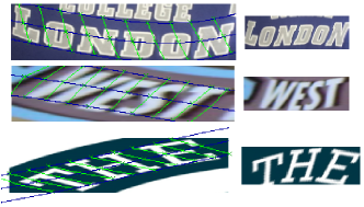
Figure 1: Examples from test data set. Left side is the original image and the blue curve is predicted with STN, then comes the controlpoints. Right side is the rectified image.

For bidirectional decoder in STR, ASTERShi et al. (2018) have implemented the left-to-right and right-to-left decoding module independently, which means the two decoders are optimized separately. The works of MORANLuo et al. (2019) and ESIRZhan and Lu (2019) all follow ASTER. However, the forward and backward decoding are (almost) identical and shares much common knowledge, the separate optimization may cause redundancy and low efficiency. Another improvement in this paper is to cut down the two independent forward and backward decoding layer into only one layer network.

The main contributions of this paper is listed as follows: 1) The finer rectification network is more flexible for scene text distortion modeling and correction. 2) A novel bidirectional decoder is equal or outperforming than the two dependent opposite direction decoder with only one decoding network. 3) With the rectification method and simplified decoder, this end-to-end model achieves state-of-the-art performance on a number of standard benchmarks.

2 Related Work

Existing works on STR can be roughly divided into traditional and deep learning based methods.

Most traditional STR work follow a bottom-up pipeline that first detects and recognizes individual character and then links up the recognized characters into words or text lines by language models. For example, Bissacco et al. (2013) uses a fully connected network for character recognition and Jaderberg et al. (2014a) uses CNNs to recognize unconstrained character. These bottom-up methods need to localize each individual characters, which is costly both for location labeling and training. Besides, these methods also prone to errors such as overlaps between adjacent characters.

Deep learning methods have dominated STR in recent years. Jaderberg et al. (2016) start to take STR as a word classification problem by CNN model which is constrained to the pre-defined vocabulary. Later, various sequence-to-sequence models Shi et al. (2016a, b, 2018); Zhan and Lu (2019), which is believed to embed the language model in the decoding layer, are applied for STR. Connectionist Temporal Classification (CTC)Shi et al. (2016a) in the decoding layer is later changed into attention based modelsCheng et al. (2018); Shi et al. (2018). VGGSimonyan and Zisserman (2014) in the feature extraction layer is later tended into ResNetHe et al. (2016). FANCheng et al. (2017) developed a focusing attention mechanism to improve the performance of general attention-based encoder-decoder framework.

The rectification in STR models based on the spatial transform network (STN), which improve the recognition accuracy while require no hand crafted features or extra annotations. Risnumawan et al. (2014) adopts the thin-plate spline (TPS) transformation based on STN for scene text distortion correction. ASTER uses TPS based on STN to rectify the warped image, the points on two sides are predicted without any constraint, two independent decoders was exploited. ESIR extends the rectification to an iterative way, however, the two points on each of the predicted line is not easy to calculate because the root may not exist, which happens when the line and curve doesn’t intersect with each other. Besides, the iteration may be not necessary.

3 The Proposed Method

This section presents the proposed recognition model for scene text including grid rectification module, sequence recognition network and the implementation details.

3.1 Rectification Network

thin plate spline based Spatial Transformation Network(STN) is used in our rectification module. The prediction of control points $C\in\mathbb{R}^{M\times N\times 2}$ is essential to the output of the rectification network. $C=\{C_{1},C_{2},\cdots,C_{M}\},C_{i}\in\mathbb{R}^{N\times 2}$.

3.1.1 Smooth Grid Localization

Since most characters in 2D scene text images are along a straight line or a smooth curve, the control points has the same trend, a polynomial curve is effective to estimate the tendency of text layout. We can use the curve with a bias to estimate each line of control points $C_{i}$.

The text line tendency along the characters can be predicted with a polynomial of order $W$ as follow:

$$\begin{split}\bar{y}(x)=&\bm{a}\bm{X}=\sum_{k=1}^{W}{a_{k}*x^{k}}\\ =&a_{1}\cdot x+a_{2}\cdot x^{2}+\cdots+a_{W}\cdot x^{W}\end{split}$$ (1)

where $\bm{a}=(a_{1},a_{2},\cdots,a_{W}),\bm{X}=(x,x^{2},\cdots,x^{W})$.

With the i-th line of x axis coordinate of the control points and a different bias $b_{i}$ generated by STN localization network, the j-th y axis coordinate of the control points on i-th line can be determined by:

$$\begin{split}y_{j}=&b_{i}+\bar{y}(x_{ij})=b_{i}+\bm{a}\bm{X}_{ij}\\ =&b_{i}+\sum_{k=1}^{W}{a_{k}\cdot x_{ij}^{k}}\end{split}$$ (2)

where $\bm{a}$ is the same between each $C_{i}$. After this elementwise operation, we can get the whole coordinate of each line of control points $C_{i}=\{(x_{j},y_{j})\},i\in\{1,2,\cdots,M\},j\in\{1,2,\cdots,N\}$.

These control points in $C$ divide the 2D plane into $M\times N$ grids, and if the x and y coordinates are predicted directly, the parameters needed is $2M\times N$, however, $M\times N+W$ parameters is enough with the proposed method for $W\ll M\times N$. The tendency of the whole control points stay the same while keeping the text line smooth.

Another intuitive way to see how these points are generated is that they are sampled from the predicted lines, and the lines are parallel to each other for the only difference is the bias.

Layers	Out Size	Configurations
conv1	$32\times 64$	32
conv2	$16\times 32$	64
conv3	$8\times 16$	64
conv4	$4\times 8$	128
conv5	$2\times 4$	128
conv6	$1\times 2$	256
FC1	256
FC2	$M\times N+M+W$

Table 1: The structure of the Rectification Network. Each conv layer is followed by a Relu and maxpooling layer, conv’s kernel size is $3\times 3$

3.1.2 TPS based Rectification

The target points $\bm{C}^{\prime}=\{\bm{C}^{\prime}_{i}\},1\leq i\leq M$ can be initialized as

$$\bm{C}^{\prime}_{i}=\left\{[\frac{j}{N},\frac{i}{M}],1\leq j\leq N\right\}$$ (3)

After we get the control points $\bm{C}$, the transformation mapping matrix $\bm{T}\in\mathbb{R}^{(M\times N+3)\times 2}$ can be calculated by

$$\bm{T}=\left[\begin{matrix}\bm{S}&\bm{1}_{M\times N}&\bm{C}\\ \bm{1}^{T}_{M\times N}&\bm{0}&\bm{0}\\ \bm{C}^{T}&\bm{0}&\bm{0}\\ \end{matrix}\right]^{-1}\cdot\left[\begin{array}[]{c}\bm{C}^{\prime}\\ \bm{0}\\ \bm{0}\end{array}\right]$$ (4)

where $\bm{S}=\{s_{ij}\}\in\mathbb{R}^{(M\times N)\times(M\times N)}$, $s_{ij}=\phi(\Delta c)$, $\Delta c$ is the difference of every two element in $\bm{C}$ and $\phi(c)=c^{2}\log c$. the $\bm{C}$ here has the size of $(M\times N)\times 2$.

For every pixel $p^{\prime}$ from the warped image, the corresponding pixel $p$ on the rectified image is

$$\bm{p}^{\prime}=\bm{T}\left[\begin{array}[]{c}1\\ \bm{p}\\ \phi(\bm{p}-\bm{c}_{11})\\ \cdots\\ \phi(\bm{p}-\bm{c}_{M\times N})\\ \end{array}\right]$$ (5)

Although this can be seen as an extension of the two-line control points adopted by Aster and Esir, this method only need to directly predict half amount of coordinates besides the weight and bias parameters. Another advantage of this method is that the generated coordinates maintain a smooth boundary. These two features do help when the rows and columns of the control points increase.

3.2 Recognition Network

The whole pipeline of the recognition network mainly follows the work of AsterShi et al. (2018). Considering the redundant two independent opposite-direction decoder, we simply exploit one decoding layer with a direction embedding to replace the two independent decoder. Figure 2 is a demonstration of the recognition network architecture.

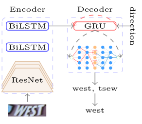
Figure 2: Framework of Recognition Network. Here is a illustration of k=2 beam search for bidirectional decoding. the red arrows denote forward decoder and the blue is backward. the two orange nodes in red dashed boxes is the current candidates.

3.2.1 Encoder

The encoder is a common CRNN architecture with ResNet as the feature extractor followed by two layers of BiLSTM. A 53-layer residual network is used to extract features, where each residual unit consists of a $1\times 1$ convolution and a $3\times 3$ convolution operations. The first two residual blocks are down-sampled with $2\times 2$ stride while the left three with $2\times 1$ stride.

3.2.2 Bidirectional Decoder

The previous works on STR with a bidirectional decoder all treat the forward and backward parts separately. However, it is obvious that forward and backward processes are almost the same, which means nearly half of the decoder network parameters are redundant. So in this section, we propose a new method to decode the sequence context information bidirectionally with only one decoder.

We need to capture the direction information for the unique decoder network, so the directional embedding is added apart from the one hot embedding.

After the GRU network iterate for T steps, a sequence $(y_{1},y_{2},\cdots,y_{T})$ is predicted. the context information $c_{t}$ can be encoded with the following attention mechanism:

$$\begin{split}p_{t,i}&=\bm{w}^{T}\tanh(\bm{W}\bm{s}_{t-1}+\bm{V}\bm{h}_{i}+b)\\ \alpha_{t,i}&=e^{p_{t,i}}/\sum_{i^{\prime}=1}^{n}{e^{p_{t,i^{\prime}}}}\\ \bm{c}_{t}&=\sum_{i=1}^{n}\alpha_{t,i}\bm{h}_{i}\end{split}$$ (6)

where $s_{t-1}$ is the internal state. After the attentional context is generated, we need to combine the embedded information. Different from ordinarily concatenating the context with one-hot embedding $f$, here we add one more direction embedding $d$ to distinguish forward and backward decoding process.

$$\begin{split}(\bm{x}_{t},\bm{s}_{t})=\text{GRU}(\bm{s}_{t-1},\text{cat}(&\bm{c}_{t},f(y_{t-1})+\\ &d(forward/backward)))\end{split}$$ (7)

where $x_{t}$ is used to predict $y_{t}\sim\text{softmax}(\bm{W}_{o}\bm{x}_{t}+b_{o})$.

The loss function of the bidirectional decoder is:

$$Loss=\lambda l_{forward}+(1-\lambda)l_{backward}$$ (8)

where $\lambda$ is a scaling factor used to define the importance between the forward and backward losses.

In the inference stage, we use beam-search with k candidates to increase the accuracy of decoding.

3.3 Implementation Details

The input image is resized to $36\times 128$ and the rectified image or the input of encoder is resized to $32\times 100$ pixels. Table 2 is the detailed architecture of the sequence recognition network. $\lambda=0.7$ is configured for forward loss weight, the candidate of beam-search is $k=5$. the batch size is 64.

	Layers	Out Size	Configurations
Encoder	Input	$32\times 100$	k3, s1, 32
	Block1	$16\times 50$	k3, s2, 64
	Block2	$8\times 25$	k3, s2, 128
	Block3	$4\times 25$	k3, s$2\times 1$, 256
	Block4	$2\times 25$	k3, s$2\times 1$, 512
	Block5	$1\times 25$	k3, s$2\times 1$, 512
	BiLSTM	25	$256\times 2$ hidden units
	BiLSTM	25	$256\times 2$ hidden units
Decoder
	GRU	*	256 attention units, 256 hidden units

Table 2: Architecture of Recognition Network. Each of the block is a residual one, the attentional GRU decoder is a bidirectional decoding layer.

The Embedding dimension is 512, the target 68 characters covers 10 digits, lower case letters and 32 ASCII punctuations. The direction embedding is the same across all the 512 dimensions.

4 Experiments

In this section we show the various training and evaluation datasets and the extensive experiments results.

Methods	IIIT5k	SVT	IC03	IC13	IC15	SVTP	CUTE
Jaderberg et al. (2016)	-	80.7	93.1	90.8	-	-	-
Shi et al. (2016a)	81.2	82.7	91.9	89.6	-	-	-
Shi et al. (2016b)	81.9	81.9	90.1	88.6	-	71.8	59.2
Lee and Osindero (2016)	78.4	80.7	88.7	90.0	-	-	-
FAN	87.4	85.9	94.2	93.3	70.6	-	-
ESIR	93.3	90.2	-	91.3	76.9	79.6	83.3
MORAN	91.2	88.3	95.0	92.4	76.1	78.5	79.5
ASTER	93.4	89.5	94.5	91.8	77.8	79.7	81.9
Firbarn	93.4	89.8	93	92.7	81.3	80.8	86.1

Table 3: Recognition results comparison to state-of-the-art. Some methods use private dataset and achieve outperforming results, which are not fair and exclude in this comparison. the configure for rectification grid size is $3\times 10$ and the curve order is 4.

4.1 Datasets

We train the model on 2 general datasets, then evaluate on 7 benchmarks, which consist of 4 regular text datasets and 3 irregular text datasets, to show its rectification ability on curved, distorted and oriented text. A brief description of these datasets is as follows.

4.1.1 Training Datasets

Real-world labeling data is costly, following most scene text recognition works, we use the synthetic data as an alternative. Specifically, we train the model on the following two datasets, no more data is used.

• Synth90K Jaderberg et al. (2014b) contains about 7.2 million training images and it has been widely used for training scene text recognition models. After cropping with the lexicon, 9 million images are used for training.

• SynthText Gupta et al. (2016) is the synthetic image dataset that was created for scene text detection research. It has been widely used for scene text recognition research as well by cropping text image patches using the provided annotation boxes. 7 million cropped images are for training.

4.1.2 Evaluation Datasets

• IIIT5K-Words (IIIT5K) Mishra et al. (2012) contains 3,000 images for testing, which are cropped from online scene texts images.

• Street View Text (SVT) Wang et al. (2011) consists of 647 testing images, which are collected from the Google Street View. Many images are heavily distorted by noise or low-resolution.

• ICDAR 2003 (IC03) Lucas et al. (2003) contains 860 images of cropped words after filtering. Following Wang et al. (2011), words with non-alphanumeric characters or less than three are filtered.

• ICDAR 2013 (IC13) Karatzas et al. (2013) inherits most of its data from IC03 and covers 1,015 cropped word images in total.

• ICDAR 2015 (IC15) Karatzas et al. (2015) is collected via Google Glasses without careful positioning and focusing. 2,077 images with various corruptions in this dataset are used for testing.

• SVT-Perspective (SVTP) Quy Phan et al. (2013) is specifically proposed to evaluate the performance of perspective text recognition algorithms. It consists of 645 images for testing.

• CUTE80 (CUTE) Risnumawan et al. (2014) is designed to evaluate curved text recognition. 288 cropped images are used for testing.

4.2 Evaluation Metrics

Following the protocol and evaluation metrics that have been widely used in scene text recognition research Shi et al. (2018); Baek et al. (2019), we evaluate the model performance using the case-insensitive word accuracy. The evaluation only counts the letters and digits error, no lexicons are used.

Figure 3: Examples of the evaluation on CUTE. Left side are orignal images and the middle are rectified one. The black color denote the ground truth, red is wrong, green is right.

4.3 Comparisons with Rectification Methods

Table 3 is the full results of the comparison with previous state-of-the-art works, which shows our method is quite effective on the irregular datasets and outperform the previous results.

Order	IC15	SVTP	CUTE
2	79.2	80	80.2
3	79.3	80.6	80.5
4	79.5	80.8	81.2
5	79.9	80.8	82.6

Table 4: Compare for the curve orders.

size	IC15	SVTP	CUTE
$2\times 18$	80.6	80.8	84.6
$3\times 12$	81.2	80.6	85.2
$4\times 9$	80	79.6	83.3

Table 5: Compare for the grid size.

5 Conclusion

A finer rectification network before the general STR helps to rectify warped images. The simplified one-layer bidirectional decoder is shown to be effective with the separated two decoders. Extensive evaluations show this end-to-end model is more effective, especially on irregular scene text images. Experiments on the grid size and the order of curve show our method can improve the recognition accuracy of warped images greatly. The further work can combine more image information to predict the text boundary and train with highly-curved text.

References

- Baek et al. [2019] Jeonghun Baek, Geewook Kim, Junyeop Lee, Sungrae Park, Dongyoon Han, Sangdoo Yun, Seong Joon Oh, and Hwalsuk Lee. What is wrong with scene text recognition model comparisons? dataset and model analysis. 2019.
- Bissacco et al. [2013] Alessandro Bissacco, Mark Cummins, Yuval Netzer, and Hartmut Neven. Photoocr: Reading text in uncontrolled conditions. In Proceedings of the IEEE International Conference on Computer Vision, pages 785–792, 2013.
- Cheng et al. [2017] Zhanzhan Cheng, Fan Bai, Yunlu Xu, Gang Zheng, Shiliang Pu, and Shuigeng Zhou. Focusing attention: Towards accurate text recognition in natural images. In Proceedings of the IEEE international conference on computer vision, pages 5076–5084, 2017.
- Cheng et al. [2018] Zhanzhan Cheng, Yangliu Xu, Fan Bai, Yi Niu, Shiliang Pu, and Shuigeng Zhou. Aon: Towards arbitrarily-oriented text recognition. In Proceedings of the IEEE Conference on Computer Vision and Pattern Recognition, pages 5571–5579, 2018.
- Gupta et al. [2016] Ankush Gupta, Andrea Vedaldi, and Andrew Zisserman. Synthetic data for text localisation in natural images. In Proceedings of the IEEE Conference on Computer Vision and Pattern Recognition, pages 2315–2324, 2016.
- He et al. [2016] Kaiming He, Xiangyu Zhang, Shaoqing Ren, and Jian Sun. Deep residual learning for image recognition. In Proceedings of the IEEE conference on computer vision and pattern recognition, pages 770–778, 2016.
- Jaderberg et al. [2014a] Max Jaderberg, Karen Simonyan, Andrea Vedaldi, and Andrew Zisserman. Deep structured output learning for unconstrained text recognition. arXiv preprint arXiv:1412.5903, 2014.
- Jaderberg et al. [2014b] Max Jaderberg, Karen Simonyan, Andrea Vedaldi, and Andrew Zisserman. Synthetic data and artificial neural networks for natural scene text recognition. arXiv preprint arXiv:1406.2227, 2014.
- Jaderberg et al. [2015] Max Jaderberg, Karen Simonyan, Andrew Zisserman, et al. Spatial transformer networks. In Advances in neural information processing systems, pages 2017–2025, 2015.
- Jaderberg et al. [2016] Max Jaderberg, Karen Simonyan, Andrea Vedaldi, and Andrew Zisserman. Reading text in the wild with convolutional neural networks. International Journal of Computer Vision, 116(1):1–20, 2016.
- Karatzas et al. [2013] Dimosthenis Karatzas, Faisal Shafait, Seiichi Uchida, Masakazu Iwamura, Lluis Gomez i Bigorda, Sergi Robles Mestre, Joan Mas, David Fernandez Mota, Jon Almazan Almazan, and Lluis Pere De Las Heras. Icdar 2013 robust reading competition. In 2013 12th International Conference on Document Analysis and Recognition, pages 1484–1493. IEEE, 2013.
- Karatzas et al. [2015] Dimosthenis Karatzas, Lluis Gomez-Bigorda, Anguelos Nicolaou, Suman Ghosh, Andrew Bagdanov, Masakazu Iwamura, Jiri Matas, Lukas Neumann, Vijay Ramaseshan Chandrasekhar, Shijian Lu, et al. Icdar 2015 competition on robust reading. In 2015 13th International Conference on Document Analysis and Recognition (ICDAR), pages 1156–1160. IEEE, 2015.
- Lee and Osindero [2016] Chen-Yu Lee and Simon Osindero. Recursive recurrent nets with attention modeling for ocr in the wild. In Proceedings of the IEEE Conference on Computer Vision and Pattern Recognition, pages 2231–2239, 2016.
- Lucas et al. [2003] Simon M Lucas, Alex Panaretos, Luis Sosa, Anthony Tang, Shirley Wong, and Robert Young. Icdar 2003 robust reading competitions. In Seventh International Conference on Document Analysis and Recognition, 2003. Proceedings., pages 682–687. Citeseer, 2003.
- Luo et al. [2019] Canjie Luo, Lianwen Jin, and Zenghui Sun. Moran: A multi-object rectified attention network for scene text recognition. Pattern Recognition, 90:109–118, 2019.
- Mishra et al. [2012] Anand Mishra, Karteek Alahari, and CV Jawahar. Scene text recognition using higher order language priors. 2012.
- Quy Phan et al. [2013] Trung Quy Phan, Palaiahnakote Shivakumara, Shangxuan Tian, and Chew Lim Tan. Recognizing text with perspective distortion in natural scenes. In Proceedings of the IEEE International Conference on Computer Vision, pages 569–576, 2013.
- Risnumawan et al. [2014] Anhar Risnumawan, Palaiahankote Shivakumara, Chee Seng Chan, and Chew Lim Tan. A robust arbitrary text detection system for natural scene images. Expert Systems with Applications, 41(18):8027–8048, 2014.
- Shi et al. [2016a] Baoguang Shi, Xiang Bai, and Cong Yao. An end-to-end trainable neural network for image-based sequence recognition and its application to scene text recognition. volume 39, pages 2298–2304. IEEE, 2016.
- Shi et al. [2016b] Baoguang Shi, Xinggang Wang, Pengyuan Lyu, Cong Yao, and Xiang Bai. Robust scene text recognition with automatic rectification. In Proceedings of the IEEE Conference on Computer Vision and Pattern Recognition, pages 4168–4176, 2016.
- Shi et al. [2018] Baoguang Shi, Mingkun Yang, Xinggang Wang, Pengyuan Lyu, Cong Yao, and Xiang Bai. Aster: An attentional scene text recognizer with flexible rectification. IEEE, 2018.
- Simonyan and Zisserman [2014] Karen Simonyan and Andrew Zisserman. Very deep convolutional networks for large-scale image recognition. arXiv preprint arXiv:1409.1556, 2014.
- Wang et al. [2011] Kai Wang, Boris Babenko, and Serge Belongie. End-to-end scene text recognition. In 2011 International Conference on Computer Vision, pages 1457–1464. IEEE, 2011.
- Zhan and Lu [2019] Fangneng Zhan and Shijian Lu. Esir: End-to-end scene text recognition via iterative image rectification. In Proceedings of the IEEE Conference on Computer Vision and Pattern Recognition, pages 2059–2068, 2019.