Particle-Gibbs Sampling For Bayesian Feature Allocation Models

Abstract

Bayesian feature allocation models are a popular tool for modelling data with a combinatorial latent structure. Exact inference in these models is generally intractable and so practitioners typically apply Markov Chain Monte Carlo (MCMC) methods for posterior inference. The most widely used MCMC strategies rely on an element wise Gibbs update of the feature allocation matrix. These element wise updates can be inefficient as features are typically strongly correlated. To overcome this problem we have developed a Gibbs sampler that can update an entire row of the feature allocation matrix in a single move. However, this sampler is impractical for models with a large number of features as the computational complexity scales exponentially in the number of features. We develop a Particle Gibbs sampler that targets the same distribution as the row wise Gibbs updates, but has computational complexity that only grows linearly in the number of features. We compare the performance of our proposed methods to the standard Gibbs sampler using synthetic data from a range of feature allocation models. Our results suggest that row wise updates using the PG methodology can significantly improve the performance of samplers for feature allocation models.

1 Introduction

Bayesian feature allocation models posit that observed data is generated by a collection of latent features with the aim of obtaining an interpretable and sparse representation of the data. A concrete way to represent a feature allocation is using a binary matrix, where the rows of this matrix represent data points or observations and the columns represent features. Common prior distributions for these binary matrices include the finite dimensional Beta-Bernoulli (FBB) model and the non-parametric Indian Buffet process (IBP) (Griffiths and Ghahramani, 2011). Exact inference for models which use these prior distributions is generally intractable, so practitioners often appeal to Monte Carlo Markov Chain (MCMC) approaches. A straightforward Gibbs sampler can be derived for such models which proceeds by updating a single entry of the binary matrix conditioned on the values of the remaining entries. While relatively simple to implement, this sampler can be extremely slow to mix due to the correlation among the feature allocation variables. In this work we show that it is possible to derive a simple Gibbs sampler which updates the entire feature usage vector of a data point (row of the binary matrix) jointly. When the number features (columns of the matrix), $K$, is small this sampler is practical and can significantly improve the mixing of the MCMC chain. However, this sampler is computationally expensive, requiring $2^{K}$ evaluations of the likelihood. We show that it is possible to sample efficiently from the distribution targeted by this row Gibbs update using the Particle Gibbs (PG) methodology (Andrieu et al., 2010). Our PG sampling approach has computational complexity that scales linearly with the number of features.

In sequel we will first review Bayesian feature allocation models and the relevant prior distributions on binary matrices. Next we will describe the new row wise Gibbs update and explain how to use the PG methodology to efficiently sample from the target distribution. We then compare these new samplers to existing approaches on a range of synthetic datasets using several previously published models. Finally, we conclude with a discussion and some thoughts on future directions.

1.1 Related work

The widely used Gibbs sampler which updates the feature allocation of each data point sequentially was first introduced by Ghahramani and Griffiths (2006). Later Meeds et al. (2007) described the use of Metropolis-Hastings (MH) moves to update multiple components of the feature allocation vector for a data point. They observed that larger moves in the space of feature allocations improved mixing, though this was never formally benchmarked. While the MH move partially addresses the issue of highly correlated features, it becomes impractical as the number of features grows, as large moves proposed at random will increasingly be rejected. An alternative approach to speeding up sampling for feature allocation models was proposed by Doshi-Velez and Ghahramani (2009). The main idea of that work was to partially marginalize elements of the model to improve mixing. This is not a general strategy however, as it requires conjugacy. Wood and Griffiths (2007) proposed the use of particle filters to fit matrix factorization models using IBP priors. In contrast to our approach, they used a single pass particle filter sampling the entire feature allocation matrix. They showed that this approach could significantly outperform single entry Gibbs sampling. However, the single pass particle filter approach does not scale well to models with large numbers of data points or features due to the degeneracy of standard particle filter methods. In contrast PG algorithms are not subject to this degeneracy. Broderick et al. (2013) pointed out the predictive distribution of the feature allocation models could be written as a product of Bernoulli distributions. However, they did not appear to pursue the obvious row wise Gibbs sampler that this implies. Fox et al. (2014) proposed the use of split-merge moves to improve the mixing of features. While the sequential nature of these proposals bear some similarity to our method, they differ in that this previous work updates the columns of the feature allocation matrix as opposed to the rows. As a result they need to be interleaved with element wise Gibbs updates to obtain adequate mixing. The methods we propose in this work can be used in place of the element wise Gibbs update with the moves proposed by Fox et al. (2014) to further improve performance.

2 Methods

Here we review the basic background about feature allocation priors and introduce the standard Gibbs updating procedure. We then explain how to implement an exact Gibbs sampler for updating an entire row of the feature allocation matrix. Next we show how to construct a PG sampler to target the conditional distribution the row wise Gibbs samples from. We then discuss two strategies for improving the efficiency of the basic PG algorithm.

2.1 Notation

We use bold letters for (random) vectors, capital letters for matrices and normal fonts for (random) scalars and sets. For quantities such as an individual observation $x_{n}$, or a parameter $\theta$, which can be either scalars or vectors without affecting our methodology, we consider them as scalars without loss of generality. Given a vector $\boldsymbol{z}=(z_{1},\ldots,z_{K})$, and $i\leq j$, we use $\boldsymbol{z}_{i:j}$ to denote the sub-vector $\boldsymbol{z}_{i:j}=(z_{i},z_{i+1},\ldots,z_{j})$. For a permutation, $\boldsymbol{\sigma}$, we let $\boldsymbol{y}[\boldsymbol{\sigma}]=(y_{\boldsymbol{\sigma}(1)},\ldots,y_{\boldsymbol{\sigma}(K)})$ denote vector obtained by permuting the entries of $\boldsymbol{y}$ by $\boldsymbol{\sigma}$. For a permutation $\boldsymbol{\sigma}$ we define the inverse permutation $\boldsymbol{\sigma}^{-1}$ to be the permutation such that $(\boldsymbol{y}[\boldsymbol{\sigma}])[\boldsymbol{\sigma}^{-1}]=\boldsymbol{y}$. To simplify notation, we do not distinguish random variables from their realization. We define discrete probability distributions with their probability mass functions, and continuous probability distributions with their density functions with respect to the Lebesgue measure.

2.2 Feature allocation

Intuitively a feature allocation model ascribes a set of features that are exhibited by a set of data points $x_{n}$. At the core of these models is the combinatorial stochastic feature allocation object. To formally define a feature allocation we follow the description in Broderick et al. (2013). Let $[N]=\{1,\ldots,N\}$, then a feature allocation $f_{N}$ of $[N]$ is defined to be a multi-set of non-empty sets of $[N]$. Let $f_{N}=\{A_{1}^{N},\ldots,A_{K}^{N}\}$ where we refer to the elements $A_{k}^{N}$ as blocks. Each block represents the assignment of data points to a feature. For example consider the feature allocation $f_{3}=\{\{1\},\{1,2\},\{2,3\}\}$. In this feature allocation the first feature is exhibited by data point 1, the second feature by data points 1 and 2, and the third feature by data points 2 and 3. In contrast to partitions which are frequently used in clustering models, feature allocations do not require data points to be in mutually exclusive blocks or in fact to be in any block. If we let $z_{n,k}=\mathbb{I}(n\in A_{k}^{N})$ then we can map the feature allocation $f_{N}$ to a binary matrix $Z\in\{0,1\}^{N\times K}$. The rows of $Z$ represent data points and the columns represent features. We use the notation $\boldsymbol{z}_{n}=(z_{n,1}\ldots z_{n,K})$ to denote the $n^{\text{th}}$ row of $Z$, that is the vector indicating which features data point $n$ uses. Note that the ordering of features is arbitrary so that the matrix $Z$ is only defined up to a permutation of the columns and strictly speaking the feature allocation prior distribution is defined on the equivalence class of matrices that are identical up to a permutation of their columns. An alternative way to define this equivalence class is as the set of matrices which are equivalent when put into left ordered form (Griffiths and Ghahramani, 2011). In sequel we will abuse notation and not make the distinction between a feature allocation $f_{N}$ and its binary matrix representation $Z$.

2.3 Feature allocation prior distributions

To specify a Bayesian feature allocation model we need to define a prior distribution for the feature allocation. In this work we consider the two most widely used prior distributions for feature allocations, the Finite Beta-Bernoulli (FBB) distribution and Indian Buffet Process (IBP). Below we give: the probability mass function of these distributions; the probability that a data point $n$ exhibits feature $k$, $\rho_{n,k}$; and the predictive distribution when adding a new data point. The predictive distribution is defined as $p(f_{N+1}|f_{N})=\frac{p(f_{N+1})}{p(f_{N})}$. Let $K_{N}=|f_{N}|$ and $m_{k}=|A_{k}^{N}|=\sum_{n=1}^{N}z_{n,k}$, then these quantities are as follows:

• FBB with $K$ features

  $$p(f_{N}) = \mathbb{I}(K_{N}=K)\prod_{k=1}^{K}\frac{\Gamma(m_{k}+a)\Gamma(N-m_{k}+b)}{\Gamma(N+a+b)}$$

  $$\rho_{N+1,k} = \frac{m_{k}+a}{N+a+b}$$

  $$p(f_{N+1}|f_{N}) = \prod_{k=1}^{K}\text{Bernoulli}\left(z_{N+1,k}\middle|\rho_{N+1,k}\right)$$

• Indian Buffet Process

  $$p(f_{N}) = \frac{\alpha^{K_{N}}}{K_{N}!}\prod_{k=1}^{K_{N}}\frac{\Gamma(m_{k})\Gamma(N-m_{k}+1)}{\Gamma(N+1)}$$

  $$\rho_{N+1,k} = \frac{m_{k}}{N+1}$$

  $$p(f_{N+1}|f_{N}) = \text{Poisson}\left(K_{N+1}^{+}\left|\frac{\alpha}{N+1}\right.\right)\prod_{k=1}^{K_{N}}\text{Bernoulli}\left(z_{N+1,k}\middle|\rho_{N+1,k}\right)$$

where $K_{N+1}^{+}$ is the number of singletons (unique) features exhibited by data point $N+1$. We note that this definition of the IBP prior differs slightly from the original one defined in Ghahramani and Griffiths (2006). This construction is due to Broderick et al. (2013) and results in an exchangeable prior as the probability mass functions only depend on the number of features and size of blocks. As we will see later this is useful for defining a Gibbs sampler for updating the feature allocation variable.

2.4 Bayesian feature allocation models

To fully specify a Bayesian feature allocation model we need two additional elements. First, a set of parameters $\boldsymbol{\theta}=(\theta_{1},\ldots,\theta_{K})$ associated with the features. We will assume that $\theta_{k}$ are drawn i.i.d. from a common distribution so that the features are exchangeable. Second, we need to define a likelihood for our data $X=(x_{1},\ldots,x_{N})^{T}$ which depends on our feature allocation matrix $Z$ and the feature parameters $\boldsymbol{\theta}$. We also assume that the data points are exchangeable so the likelihood takes the form $p(X|\boldsymbol{\theta},Z)=\prod_{n=1}^{N}p(x_{n}|\boldsymbol{z}_{n},\boldsymbol{\theta})$. In order for the model to remain exchangeable we require that for any permutation, $\boldsymbol{\sigma}$, that $p(x_{n}|\boldsymbol{\theta},\boldsymbol{z}_{n})=p(\boldsymbol{x}_{n}|\boldsymbol{\theta}[\boldsymbol{\sigma}],\boldsymbol{z}_{n}[\boldsymbol{\sigma}])$. With these assumptions the full joint distribution is given by Equation 1.

$$p(X,Z,\boldsymbol{\theta})=p(Z)\left\{\prod_{k=1}^{K}p(\theta_{k})\right\}\left\{\prod_{n=1}^{N}p(x_{n}|\boldsymbol{z}_{n},\boldsymbol{\theta})\right\}$$ (1)

In general the component distributions will also depend on additional hyper-parameters which may also have prior distributions. For notational clarity we have suppressed these terms and any dependencies on these hyper-parameters.

As a concrete example consider the linear Gaussian feature allocation model.

$$Z \sim \text{IBP}(\alpha)$$

$$\theta_{k} \sim \mathcal{N}(0,\mathbf{I})$$

$$\boldsymbol{x}_{n}|\sigma,\theta_{k},\boldsymbol{z}_{n} \sim \mathcal{N}\left(\sum_{k}z_{n,k}\theta_{k},\sigma^{2}\mathbf{I}\right)$$

This model assumes the feature parameters follow a multivariate normal distribution, and the data follow a multivariate normal distribution with a mean which is the sum of the features that a data point exhibits. Note that the likelihood is invariant to permutations of the feature indexes due to the linear sum construction. This model is thus exchangeable in both data points and features.

2.5 Gibbs updates

Since data points are exchangeable we can use $p(f_{N+1}|f_{N})$ to derive a simple Gibbs sampler to update the entries of $Z$ by assuming we are observing the last data point to be assigned. Let $Z^{(-n)}=\{\boldsymbol{z}_{i}\}_{i\neq n}$ indicate the entries of $Z$ minus the $n^{\text{th}}$ row. Let $m_{k}^{(-n)}=\sum_{i\neq n}z_{i,k}$ and $\rho_{n,k}$ be defined by replacing $m_{k}$ in the definition of $\rho_{N+1,k}$ from the previous section with $m_{k}^{(-n)}$. The element wise Gibbs update takes the form given by Equation 2 for the FBB model leading to Algorithm 1 for updating a row.

$$p(z_{n,k}=1|x_{n},Z^{(-n)},\boldsymbol{\theta})\propto\rho_{n,k}\times p(x_{n}|\boldsymbol{z}_{n},\boldsymbol{\theta})$$ (2)

The update for the IBP prior is slightly more complex and is performed in two parts. We update columns for features which are also exhibited by other data points using the Gibbs update in Algorithm 1 as for the FBB. The columns for features exhibited only by the current data point, singletons, are then updated with another move which leaves the target distribution invariant. The simplest of these is to use a Metropolis-Hastings update where the number of singletons is proposed from the Poisson with parameter $\frac{\alpha}{N}$, and the corresponding feature values from their prior distributions. The methods we describe in this work only applies to the non-singleton updates, and can be used with any update for the singletons.

Algorithm 1 Sample a row of the feature allocation using the element wise Gibbs update.

1:function ElementWiseGibbsUpdate($x_{n}$, $\boldsymbol{\rho}_{n}$, $\boldsymbol{z}_{n}$, $\boldsymbol{\sigma}$)

2:     for $k\in\boldsymbol{\sigma}$ do $\triangleright$ Iterate over columns in random order.

3:         $z_{n,k}\leftarrow 0$

4:         $p_{0}\leftarrow(1-\rho_{n,k})\times p(x_{n}|\boldsymbol{z}_{n},\boldsymbol{\theta})$

5:         $z_{nk}\leftarrow 1$

6:         $p_{1}\leftarrow\rho_{n,k}\times p(x_{n}|\boldsymbol{z}_{n},\boldsymbol{\theta})$

7:         $p_{1}\leftarrow\frac{p_{1}}{p_{0}+p_{1}}$

8:         $z_{nk}\sim\text{Bernoulli}(\cdot|p_{1})$

9:     end for

10:     return $\boldsymbol{z}_{n}$

11:end function

2.6 Row wise Gibbs updates

The element wise Gibbs update has been widely used. It only requires $\mathcal{O}(K)$ evaluations of the likelihood function to update a row. However, the resulting sampler can be extremely slow to mix due to correlations between the features. The form of the predictive distributions for the FBB and IBP priors suggests an alternative Gibbs update that could potentially lead to better mixing. Rather than sample a single entry at a time, instead update an entire row, $\boldsymbol{z}_{n}$, of the feature allocation matrix. This can be done by using the update defined by Equation 3 leading to Algorithm 2 for updating a row. Again, this update only applies to the non-singleton entries when using the IBP prior.

$$p(\boldsymbol{z}_{n}=\boldsymbol{z}|X,Z^{(-n)},\boldsymbol{\theta}) \propto p(x_{n}|\boldsymbol{z}_{n},\boldsymbol{\theta})\prod_{k=1}^{K}\text{Bernoulli}\left(z_{k}\middle|\rho_{n,k}\right)$$ (3)

In order to sample from distribution defined by Equation 3 we need to enumerate all possible binary vectors of length $K$ and evaluate the likelihood function. This approach leads to a sampler with computational complexity $\mathcal{O}(2^{K})$. For moderate values of $K$, particularly if we are using the parametric FBB prior, this is a practical sampler. However, the exponential scaling in $K$ will render this approach infeasible for larger numbers of features. This is especially problematic when using the IBP prior, as $K$ varies between iterations.

Algorithm 2 Sample a row of the feature allocation using the row wise Gibbs update.

1:function RowWiseGibbsUpdate($x_{n}$, $\boldsymbol{\rho_{n}}$, $K$)

2:     $j$ $\leftarrow$ $0$ $\triangleright$ Counter for number of vectors

3:     $S$ $\leftarrow$ $()$ $\triangleright$ List to store vectors

4:     for $\boldsymbol{z}\in\{0,1\}^{K}$ do $\triangleright$ Iterate over all possible feature allocation vectors.

5:         $j$ $\leftarrow$ $j+1$

6:         $S$ $\leftarrow$ $(S,\boldsymbol{z})$ $\triangleright$ Add $\boldsymbol{z}$ to list of visited vectors

7:         $p_{j}$ $\leftarrow$ $p(x_{n}|\boldsymbol{z},\boldsymbol{\theta})\prod_{k}(1-\rho_{n,k})^{(1-z_{k})}\rho_{n,k}^{z_{k}}$

8:     end for

9:     for $i\in\{1,\dots,j\}$ do

10:         $p_{i}$ $\leftarrow$ $\frac{p_{i}}{\sum_{l=1}^{j}p_{l}}$ $\triangleright$ Normalize probabilities

11:     end for

12:     $i$ $\sim$ $\text{Categorical}(\cdot\mid\boldsymbol{p})$ $\triangleright$ Sample vector index $i$ with probability $p_{i}$

13:     $\boldsymbol{z}$ $\leftarrow$ $S_{i}$

14:     return $\boldsymbol{z}$

15:end function

2.7 Particle Gibbs updates

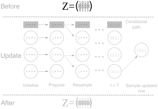
Figure 1: Illustration of the PG update procedure. Note we suppress the random ordering of features defined by $\boldsymbol{\sigma}$ for clarity. (top) Select a row for the update, shown in grey. (middle) Run a conditional particle filter and sample new row. (bottom) Update row with sample for particle filter, shown in grey. The stars (*) indicate values of the test path. We discuss how these values can be selected in Section 3.2.4.

We now describe how to sample from $p(\boldsymbol{z}_{n}=\boldsymbol{z}|X,Z^{(-n)},\boldsymbol{\theta})$ with computational complexity $\mathcal{O}(K)$ by using the Particle Gibbs (PG) methodology (Andrieu et al., 2010). PG sampling is a form of Sequential Monte Carlo (SMC) sampling (Doucet and Johansen, 2009). Like all SMC algorithms the PG approach proceeds by approximating a sequence of distribution using a set of interacting particles. Resampling is periodically used to prune particles which, informally, are exploring low probability regions. There are three key quantities that need to be defined when constructing an SMC sampler:

1. The sequence of target distributions $\{\gamma_{t}\}_{t=1}^{T}$ used to weigh the particles at each time step.

2. The sequence of proposal distributions $\{q_{t}\}_{t=1}^{T}$ used to extend particles between time steps.

3. The resampling distribution $r(\cdot|\mathbf{w}_{t-1})$.

The key difference between PG and other SMC approaches is that we are updating a set of variables which have already been instantiated. We would like to do this in way that leads to a valid kernel targeting the conditional distribution $p(\boldsymbol{z}_{n}=\boldsymbol{z}|X,Z^{(-n)},\boldsymbol{\theta})$. To accomplish this we need to include a conditional path, that is a particle trajectory which follows the sequence of choices required to generate the initial value before the update. This trajectory will always be included after the resampling steps. Thus the resampling step is conditional on including the particle representing this trajectory. Intuitively this forces the sampler to explore regions of space around the existing value. To simplify the bookkeeping and algorithm implementation we always assume the first particle is the conditional path. The PG sampler is still valid when this is done as shown by Chopin et al. (2015).

SMC algorithms are commonly used for models with a natural sequential structure, such as state space models. This in turn identifies a natural sequence of target distributions defined on an expanding state space. Our setup is non-standard in that no natural sequential structure is defined. To sample from $p(\boldsymbol{z}_{n}=\boldsymbol{z}|X,Z^{(-n)},\boldsymbol{\theta})$ we will define a sequence of distribution which updates one entry of the feature allocation vector $\boldsymbol{z}_{n}$ at each time step. Thus if we have $K$ features we will define a sequence of $T=K$ target distributions. For the FBB we take $T$ to be the fixed value of $K$ and update all elements. For the IBP $T$ is taken to be the number of elements such $m_{k}^{(-n)}>0$ and we only update the corresponding feature assignments.

At time step $t$ of the algorithm the particles will take values $\boldsymbol{\xi}_{t}\in\{0,1\}^{t}$, that is we record the sequence of binary decisions up to point $t$. In order to evaluate the likelihood term we need to set the values of the feature vector which have not been updated at time $t$. To do this we introduce an auxiliary variable which we call the the test path denoted $\bar{\boldsymbol{z}}$. We discuss and compare possible strategies for selecting $\bar{\boldsymbol{z}}$ later. An illustration of the method is given in Figure 1.

We randomly order the features before each update by a permutation $\boldsymbol{\sigma}$ so that at time $t$ we sample component $\boldsymbol{\sigma}(t)$ of the feature allocation vector. To obtain a complete feature vector to evaluate the likelihood we define the function given by Equation 4 which returns a binary vector where the entries $\boldsymbol{\sigma}(1:t)$ have been set to the sampled values and the remaining entries are set to the test path. The entries are then reordered by the inverse permutation $\boldsymbol{\sigma}^{-1}$.

$$\boldsymbol{z}(t,\boldsymbol{\sigma},\boldsymbol{\xi}_{t},\bar{\boldsymbol{z}}) = (\xi_{1},\ldots,\xi_{t},\bar{z}_{\boldsymbol{\sigma}(t+1)},\ldots,\bar{z}_{\boldsymbol{\sigma}(T)})[\boldsymbol{\sigma}^{-1}]$$ (4)

For the IBP the singleton entries are fixed to one and deterministically inserted when evaluating the likelihood.

We use the sequence of target distributions defined in Equation 5. We have $\gamma_{T}(\boldsymbol{\xi}_{T}|\boldsymbol{\rho}_{n},\boldsymbol{\sigma},\bar{\boldsymbol{z}})\propto p(\boldsymbol{z}_{n}=\boldsymbol{z}|X,Z^{(-n)},\boldsymbol{\theta})$, that it the target density at the final iteration is proportional to the density of the distribution of interest. This is the key constraint required to define a valid sequence of target distributions.

$$\gamma_{t}(\boldsymbol{\xi}_{t}|\boldsymbol{\rho}_{n},\boldsymbol{\sigma},\bar{\boldsymbol{z}}) = p(x_{n}|\boldsymbol{z}(t,\boldsymbol{\sigma},\boldsymbol{\xi}_{t},\bar{\boldsymbol{z}}),\boldsymbol{\theta})\prod_{s=1}^{t}\rho_{n\boldsymbol{\sigma}(s)}^{(1-\xi_{s})}\rho_{n\boldsymbol{\sigma}(s)}^{\xi_{s}}$$ (5)

The second component we need for our algorithm is a sequence of proposal distributions. Here we exploit the fact that our proposal space is $\{0,1\}$ and use the fully adapted proposal kernel defined in Equations 6 and 7. We use $(\boldsymbol{\xi}_{t-1},\xi_{t})$ to denote the concatenation $\xi_{t}$ to $\boldsymbol{\xi}_{t-1}$ and $\boldsymbol{\xi}_{t}=(\boldsymbol{\xi}_{t-1},\xi_{t})$.

$$q_{1}(\xi_{1}) = \frac{\gamma_{1}(\boldsymbol{\xi}_{1}|\boldsymbol{\rho}_{n},\boldsymbol{\sigma},\bar{\boldsymbol{z}})}{\sum_{\xi_{1}\in{0,1}}\gamma_{1}((\xi_{1})|\boldsymbol{\rho}_{n},\boldsymbol{\sigma},\bar{\boldsymbol{z}})}$$ (6)

$$q_{t}(\xi_{t}|\boldsymbol{\xi}_{t-1}) = \frac{\gamma_{t}(\boldsymbol{\xi}_{t}|\boldsymbol{\rho}_{n},\boldsymbol{\sigma},\bar{\boldsymbol{z}})}{\sum_{\xi_{t}\in{0,1}}\gamma_{t}((\boldsymbol{\xi}_{t-1},\xi_{t})|\boldsymbol{\rho}_{n},\boldsymbol{\sigma},\bar{\boldsymbol{z}})}$$ (7)

Given our choice of proposal and target distributions the incremental weight functions are defined by Equations 8 and 9. To reduce computational overhead $p(x_{n}|\boldsymbol{z}(t,\boldsymbol{\sigma},\boldsymbol{\xi}_{t},\bar{\boldsymbol{z}}),\boldsymbol{\theta})$ can be cached to avoid re-evaluation of the likelihood term in the denominator of Equation 9.

$$w_{1}(\boldsymbol{\xi}_{1}) = \frac{\gamma_{1}(\boldsymbol{\xi}_{1}|\boldsymbol{\rho}_{n},\boldsymbol{\sigma},\bar{\boldsymbol{z}})}{q_{1}(\xi_{1})}$$ (8)

$$= \sum_{\xi_{1}\in\{0,1\}}\gamma_{1}((\xi_{1})|\boldsymbol{\rho}_{n},\boldsymbol{\sigma},\bar{\boldsymbol{z}})$$

$$w_{t}(\boldsymbol{\xi}_{t}|\boldsymbol{\xi}_{t-1}) = \frac{\gamma_{t}(\boldsymbol{\xi}_{t}|\boldsymbol{\rho}_{n},\boldsymbol{\sigma},\bar{\boldsymbol{z}})}{\gamma_{t-1}(\boldsymbol{\xi}_{t-1}|\boldsymbol{\rho}_{n},\boldsymbol{\sigma},\bar{\boldsymbol{z}})q_{t}(\xi_{t}|\boldsymbol{\xi}_{t-1})}$$ (9)

$$= \sum_{\xi_{t}\in\{0,1\}}\frac{\gamma_{t}((\boldsymbol{\xi}_{t-1},\xi_{t})|\boldsymbol{\rho}_{n},\boldsymbol{\sigma},\bar{\boldsymbol{z}})}{\gamma_{t-1}(\boldsymbol{\xi}_{t-1}|\boldsymbol{\rho}_{n},\boldsymbol{\sigma},\bar{\boldsymbol{z}})}$$

The final component we need to define our PG algorithm is a resampling distribution. For simplicity we use multinomial resampling, however more sophisticated approaches such as stratified sampling could also be use. Our resampling distribution deterministically includes the conditional path, which we arbitrarily assign to particle index 1. The conditional multinomial resampling distribution is given by Equation 10 where $\mathbf{a}\in\{1,\ldots,P\}^{P}$ is the vector of ancestor indices, $\boldsymbol{w}$ the vector of normalized particle weights and $P$ is the number of particles.

$$r(\mathbf{a}|\boldsymbol{w}) = \mathbb{I}\left(a_{1}=1\right)\prod_{i=2}^{P}\prod_{j=1}^{P}w^{\mathbb{I}\left(a_{i}=j\right)}_{i}$$ (10)

Algorithm 3 Sample a row of the feature allocation using the particle Gibbs update.

1:function ParticleGibbsUpdate($x_{n}$, $\boldsymbol{z}_{n}$, $\boldsymbol{\sigma}$, $\boldsymbol{\rho^{n}},\bar{\boldsymbol{z}}$)

2:     $\boldsymbol{\xi}_{T}^{1}\leftarrow\boldsymbol{z}_{n}[\boldsymbol{\sigma}]$ $\triangleright$ Set conditional path

3:     for $t\in\{1,\ldots,T-1\}$ do

4:         $\boldsymbol{\xi}_{t}^{1}\leftarrow(\boldsymbol{\xi}_{T}^{1})_{1:t}$ $\triangleright$ First particle of each generation matches conditional path

5:     end for

6:     for $i\in\{2,\ldots,P\}$ do $\triangleright$ Initialize unconditional particles

7:         $\xi_{1}^{i}\sim q_{1}(\cdot)$

8:         $\boldsymbol{\xi}_{1}^{i}\leftarrow(\xi_{1}^{i})$

9:     end for

10:     for $i\in\{1,\ldots,P\}$ do $\triangleright$ Initialize incremental importance weights

11:         $\widetilde{w}_{1}^{i}\leftarrow w_{1}(\boldsymbol{\xi}_{1}^{i})$

12:     end for

13:     for $i\in\{1,\ldots,P\}$ do $\triangleright$ Compute normalized weights

14:         $w_{1}^{i}\leftarrow\frac{\widetilde{w}_{1}^{i}}{\sum_{j}\widetilde{w}_{1}^{j}}$

15:     end for

16:     for $t\in\{2,\ldots,T\}$ do

17:         if $(P\sum_{i}(w_{t-1}^{i})^{2})^{-1}<\tau$ then $\triangleright$ Resample only if the relative ESS below threshold $\tau$

18:              $\mathbf{a}\sim r(\cdot|\mathbf{w}_{t-1})$ $\triangleright$ Conditional resampling

19:              $\mathbf{w}_{t-1}\leftarrow(1,\ldots,1)$ $\triangleright$ Reset incremental weights to one

20:         else

21:              $\mathbf{a}\leftarrow(1,2,\ldots,P)$ $\triangleright$ Resampling skipped set $\mathbf{a}$ to identity map

22:         end if

23:         for $i\in\{2,\ldots,P\}$ do $\triangleright$ Propose new feature usage for feature $\boldsymbol{\sigma}(t)$

24:              $\xi_{t}^{i}\sim q_{t}(\cdot|\boldsymbol{\xi}_{t-1}^{a_{i}})$

25:              $\boldsymbol{\xi}_{t}^{i}\leftarrow(\boldsymbol{\xi}_{t-1}^{a_{i}},\xi_{t}^{i})$

26:         end for

27:         for $i\in\{1,\ldots,P\}$ do

28:              $\widetilde{w}_{t}^{i}\leftarrow w_{t-1}^{a_{i}}w_{t}(\boldsymbol{\xi}_{t}^{i}|\boldsymbol{\xi}_{t-1}^{a_{i}})$ $\triangleright$ Update incremental importance weights

29:         end for

30:         for $i\in\{1,\ldots,P\}$ do

31:              $w_{t}^{i}\leftarrow\frac{\widetilde{w}_{t}^{i}}{\sum_{j}\widetilde{w}_{t}^{j}}$ $\triangleright$ Compute normalized weights

32:         end for

33:     end for

34:     $\boldsymbol{z}\sim\sum_{i=1}^{P}w_{T}^{i}\delta_{\boldsymbol{\xi}_{T}^{i}}(\cdot)$ $\triangleright$ Sample updated feature allocation

35:     $\boldsymbol{z}\leftarrow\boldsymbol{z}[\boldsymbol{\sigma}^{-1}]$ $\triangleright$ Reorder sampled feature allocation vector by inverse of $\boldsymbol{\sigma}$

36:     return $\boldsymbol{z}$

37:end function

2.8 Annealed target distributions

One potential pitfall of the target distribution is that due to the correlation among features, it is difficult to change a feature from its current values. This will be particularly acute if there is a need to move through a low probability configuration. A simple strategy to mitigate this is to consider an different family of target distributions which anneals the likelihood defined in Equation 11.

$$\gamma_{\beta,t}(\boldsymbol{\xi}_{t}|\boldsymbol{\rho}_{n},\boldsymbol{\sigma},\bar{\boldsymbol{z}})= p(x_{n}|\boldsymbol{\xi}_{t},\boldsymbol{\theta})^{{\left(\frac{t}{T}\right)^{\beta}}}\prod_{s=1}^{t}\rho_{n\boldsymbol{\sigma}(s)}^{(1-\xi_{s})}\rho_{n\boldsymbol{\sigma}(s)}^{\xi_{s}}$$ (11)

It can easily be checked that $\gamma_{\beta,T}(\boldsymbol{z})\propto p(\boldsymbol{z}_{n}=\boldsymbol{z}|X,Z^{(-n)},\boldsymbol{\theta})$ so this sequence of target densities does indeed target the correct distribution. Also note, the original sequence of densities is recovered if $\beta=0$.

2.9 Discrete particle filtering

SMC algorithms are known to be inefficient in cases where the target distribution is discrete. This is due to the computation and storage of redundant particles. Fearnhead and Clifford (2003) addressed this problem by designing an SMC approach tailored to discrete state spaces. The key difference is that their approach deterministically expands each particle to test all available extensions, which is possible due to the discrete nature of the space. In order to avoid storing an exponentially expanding system of particles, they introduce an approach to deterministically keep particles with high weights while resampling from those with low weights. Their approach guarantees that no more that $|\mathcal{X}|M$ particles will be created, where $\mathcal{X}$ is the discrete state space and $M$ is a user specified value. Whiteley et al. (2010) later showed that this approach could be adapted to the Particle Gibbs framework. We refer to this approach as the discrete particle filter (DPF). In practice we use a slightly different version which was proposed by Barembruch et al. (2009). This version sets the expected number of particles to $M$ instead of fixing it at exactly $M$. We have found this implementation to be more stable numerically. The resampling procedure is outlined in Algorithm 4.

There is no proposal densities in the DPF algorithm so we obtain a different set of weight functions from the PG algorithm which are given by Equations 12 and 13. As for the PG algorithm it is useful to cache $p(x_{n}|\boldsymbol{z}(t,\boldsymbol{\sigma},\boldsymbol{\xi}_{t},\bar{\boldsymbol{z}}),\boldsymbol{\theta})$ to avoid re-evaluation of the likelihood term in the denominator. When using annealing the corresponding target densities are substituted in the weight functions. The full details of the DPF are given in Algorithm 5. Again to simplify the bookkeeping our proposed algorithm always assigns the conditional path to the first particle, and this is enforced during resampling.

$$w_{1}(\boldsymbol{\xi}_{1}) = \gamma_{1}(\boldsymbol{\xi}_{1}|\boldsymbol{\rho}_{n},\boldsymbol{\sigma},\bar{\boldsymbol{z}})$$ (12)

$$w_{t}(\boldsymbol{\xi}_{t}|\boldsymbol{\xi}_{t-1}) = \frac{\gamma_{t}(\boldsymbol{\xi}_{t}|\boldsymbol{\rho}_{n},\boldsymbol{\sigma},\bar{\boldsymbol{z}})}{\gamma_{t-1}(\boldsymbol{\xi}_{t-1}|\boldsymbol{\rho}_{n},\boldsymbol{\sigma},\bar{\boldsymbol{z}})}$$ (13)

Algorithm 4 Conditional resampling for DPF.

1:function ResampleDPF(w, $M$, $P$)

2:     $c$ $\leftarrow$ findRoot($\sum_{i=1}^{P}\text{min}(1,xw_{i})-M$) $\triangleright$ Find unique root $x$ to equation on right

3:     $\mathbf{a}\leftarrow\{1\}$ $\triangleright$ First index is conditional path

4:     $j\leftarrow 1$ $\triangleright$ Initialize number of retained particles

5:     if $w_{1}\geq\frac{1}{c}$ then

6:         $\widetilde{w}_{1}\leftarrow w_{1}$

7:     else

8:         $\widetilde{w}_{1}\leftarrow\frac{1}{c}$

9:     end if

10:     for $i\in\{2,\ldots,P\}$ do

11:         if $w_{i}\geq\frac{1}{c}$ then $\triangleright$ Retain particles with large weights

12:              $\mathbf{a}\leftarrow(\mathbf{a},i)$

13:              $\widetilde{w}_{j}\leftarrow w_{i}$

14:              $j\leftarrow j+1$

15:         else$\triangleright$ Resample particles with small weights

16:              $U\sim\text{Uniform}(\cdot\mid[0,1])$

17:              if $c\,w_{i}\geq U$ then

18:                  $\mathbf{a}\leftarrow(\mathbf{a},i)$

19:                  $\widetilde{w}_{j}\leftarrow\frac{1}{c}$

20:                  $j\leftarrow j+1$

21:              end if

22:         end if

23:     end for

24:     for $i\in\{1,\ldots,j\}$ do

25:         $w_{i}^{new}\leftarrow\frac{\widetilde{w}_{i}}{\sum_{l=1}^{j}\widetilde{w}_{l}}$ $\triangleright$ Normalize new weights

26:     end for

27:     return $\mathbf{a}$, $\textbf{w}^{new}$, $j$

28:end function

Algorithm 5 Sample a row of the feature allocation using the discrete particle filter update.

1:function DiscreteParticleFilter($x_{n}$, $\boldsymbol{z}_{n}$, $\boldsymbol{\sigma}$, $\boldsymbol{\rho^{n}},\bar{\boldsymbol{z}}$, $M$)

2:     $\boldsymbol{\xi}_{T}^{1}\leftarrow\boldsymbol{z}[\boldsymbol{\sigma}]$ $\triangleright$ Set conditional path

3:     for $t\in\{1,\ldots,T-1\}$ do

4:         $\boldsymbol{\xi}_{t}^{1}$ $\leftarrow$ $(\boldsymbol{\xi}_{T})_{1:t}$ $\triangleright$ First particle of each generation matches conditional path

5:         $\boldsymbol{\xi}_{t}^{2}$ $\leftarrow$ $(\boldsymbol{\xi}_{t-1}^{1},1-(\boldsymbol{\xi}_{t}^{1})_{t})$ $\triangleright$ Expand conditional path with alternate feature value for time $t$

6:     end for

7:     $P\leftarrow 2$ $\triangleright$ Initialize number of particles

8:     for $i\in\{1,2\}$ do

9:         $\widetilde{w}_{1}^{i}\leftarrow w_{1}(\boldsymbol{\xi}_{1}^{i})$ $\triangleright$ Initialize incremental importance weights

10:     end for

11:     for $i\in\{1,2\}$ do

12:         $w_{1}^{i}\leftarrow\frac{\widetilde{w}_{1}^{i}}{\sum_{j}\widetilde{w}_{1}^{j}}$ $\triangleright$ Compute normalized weights

13:     end for

14:     for $t\in\{2,\ldots,T\}$ do

15:         if $P>M$ then $\triangleright$ Check if there are too many particles

16:              $\mathbf{a}$, $\boldsymbol{w}_{t}$, $P$ $\leftarrow$ ResampleDPF($\boldsymbol{w}_{t}$, $M$, $P$) $\triangleright$ Resample using Algorithm 4

17:         else

18:              $\mathbf{a}\leftarrow(1,\ldots,P)$ $\triangleright$ Set ancestor indices to identity map

19:         end if

20:         $j\leftarrow 2$ $\triangleright$ Track number of particles

21:         for $i\in\{2,\ldots,P\}$ do

22:              for $z\in\{0,1\}$ do

23:                  $j\leftarrow j+1$

24:                  $\boldsymbol{\xi}_{t}^{j}\leftarrow(\boldsymbol{\xi}_{t-1}^{a_{i}},z)$ $\triangleright$ Expand unconditional particles

25:              end for

26:         end for

27:         $P\leftarrow j$ $\triangleright$ Update number of particles

28:         for $i\in\{1,\ldots,P\}$ do

29:              $\widetilde{w}_{t}^{i}\leftarrow w_{t-1}^{a_{i}}w_{t}(\boldsymbol{\xi}_{t}^{i}|\boldsymbol{\xi}_{t-1}^{a_{i}})$ $\triangleright$ Update incremental importance weights

30:         end for

31:         for $i\in\{1,\ldots,P\}$ do

32:              $w_{t}^{i}\leftarrow\frac{\widetilde{w}_{t}^{i}}{\sum_{j}\widetilde{w}_{t}^{j}}$ $\triangleright$ Compute normalized weights

33:         end for

34:     end for

35:     $\boldsymbol{z}\sim\sum_{i=1}^{P}w_{T}^{i}\delta_{\boldsymbol{\xi}_{T}^{i}}(\cdot)$ $\triangleright$ Sample updated feature allocation

36:     $\boldsymbol{z}\leftarrow\boldsymbol{z}[\boldsymbol{\sigma}^{-1}]$ $\triangleright$ Reorder sampled feature allocation vector by inverse of $\boldsymbol{\sigma}$

37:     return $\boldsymbol{z}$

38:end function

3 Results

We first demonstrate the potential slow mixing of the standard Gibbs sampler on a toy dataset and illustrate how the row wise Gibbs updates can alleviate this problem. Next we explore how to tune the parameters of the PG and DPF samplers. We then compare the behaviour of the Gibbs sampler and our proposed methods on a number of synthetic datasets.

We have compared the performance of the Gibbs, Row Gibbs (RG), Particle Gibbs (RG) and Discrete Particle Filter (DPF) using three models. The first model we tested with was the Linear Gaussian (LG) model, which has been widely used in the IBP literature (Griffiths and Ghahramani, 2011). The second model we considered was the Latent Feature Relational Model (LFRM) proposed by Miller et al. (2009). The final model we consider is a modified version of the PyClone model used for inferring population structure from admixed data in cancer genomics (Roth et al., 2014). The original PyClone model clusters sets of mutations which appear in a similar proportion of cells. We have modified this model to use feature allocations to indicate which cell populations have each mutation. Full details of the models and the updates used for parameters are in the Section 5.1.

When comparing methods we applied the Friedman test to see if there were any significant difference in performance between the methods (p-value $<$ 0.001). If the Friedman test was significant we then applied the post-hoc Nemenyi test with a Bonferroni correction to all pairs of models to determine which models showed significantly different performance from each other (p-value $<$ 0.001) (Demšar, 2006). All statements of significance are with respect to this test. Because the samplers have different computational complexity per iteration, we report the results using wall clock time instead of per iteration. This ensures a fair comparison, as for example, we can perform many more updates using the Gibbs sampler than the PG sampler in a given time interval. We report the relative log density when comparing methods to better represent how far away from convergence the samplers are. Let $\hat{\ell}$ be the log density of the data under the true parameters used for simulation and $\ell$ the observed log density. The relative log density is given by $\frac{\ell-\hat{\ell}}{\hat{\ell}}$.

Code implementing the samplers and models is available online at https://github.com/aroth85/pgfa. All experiments were done using version 0.2.2 of the software. Code for performing the experiments is available online at https://github.com/aroth85/pgfa_experiments.

3.1 Row updates improve mixing

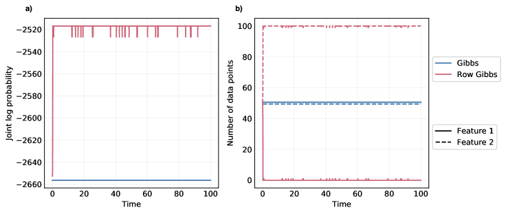
Figure 2: Comparison of element wise Gibbs to row Gibbs sampler. a) Log joint probability of the samplers over time. b) Number of data points assigned to each feature over time. Lines for the Gibbs sampler are jittered away from 50 for visibility.

To illustrate the potential benefits of using row wise updates, we first consider a simple pedagogical example. We simulated $N=100$ data points from the linear Gaussian model with $D=1$, $K=2$, $\tau_{v}=0.25$, and $\tau_{x}=25$. We set the value of the feature parameters $V$ to be 100 for both features with half of the data points using the first feature and half using the second feature. For inference we used the FBB prior with $K=2$, $a=0.5$ and $b=1$. This prior distribution for the feature allocation heavily favours the configuration where all data points use one feature and the other is not used. Because both features have identical values, there is no difference is likelihood for a data point to use one feature or the other. Thus, if a sampler is mixing efficiently it should quickly assign all data points to one feature and none to the other. We ran both the element wise Gibbs and row wise Gibbs samplers for 100 seconds recording the value of the log joint probability and number of data points that used each feature at each iteration. We set all model parameters except the feature allocation to their true values, and did not update them in contrast to the remaining experiments where the feature parameters are updated. We show the trace of the log joint probability in Figure 2 a). The element wise Gibbs sampler (blue) is clearly trapped in a local mode from initialization and cannot move away from the initial configuration. This is due to the need for the element wise Gibbs sampler to traverse a region of low probability to use the other feature. Specifically, a data point must use both features or neither feature in one iteration before it can then only use the other feature in the next iteration. Figure 2 b) supports this hypothesis as we see that the number of data points using each feature never changes over the course of sampling. In contrast the row wise Gibbs sampler (red) rapidly increases the joint probability Figure 2 a) and moves all data points to a single feature Figure 2 b). This contrived example clearly illustrates the potential for slow mixing that element wise updates can cause and that row wise updates can solve the problem. We will see that this behaviour is a general phenomenon of the element wise Gibbs sampler, even when the initialization is not constructed to be adversarial as in this case.

3.2 Setting tuning parameters

The PG and DPF samplers have a number of tuning parameters which affect performance. We explored the impact these parameters have on performance using synthetic data generated from the LG model. We generated four datasets and four sets of initial parameter values. For all combinations of datasets and initial parameters we performed five random restarts of the sampler. Thus we executed 80 chains for each method considered, all with the same data and parameter initialization. Data was simulated from the LG model using the FBB prior with $\alpha=2$, $\tau_{v}=0.25$, $\tau_{x}=25$, $D=10$, $K=20$ and $N=100$. These parameters were chosen to generate datasets where we would expect the sampler to converge to the true parameter values used for simulation. We randomly assigned 10% of the data matrix to be missing and used these entries to compute root mean square reconstruction error (RMSE). For each experiment we varied a single tuning parameter, setting the remaining parameters to default values, namely an annealing power of 1.0, a number of particles of 20, a resampling threshold of 0.5, and test paths consisting of a vector of zeros.

3.2.1 Number of particles

The first parameter we explore is the number of particles. For standard SMC algorithms a large number of particles are typically used, as this parameter ultimately controls the quality of the Monte Carlo approximation. In contrast to standard SMC, the Particle Gibbs framework is less sensitive to the number of particles. This is primarily a result of the fact many conditional SMC (cSMC) moves can be used within a sampling run, in contrast to the one shot approach of SMC. For our particular problem the length of the cSMC runs also tends to be short because we rarely expect very large numbers of features to be used in the model. As a result, our updates will also be less sensitive to path degeneracy.

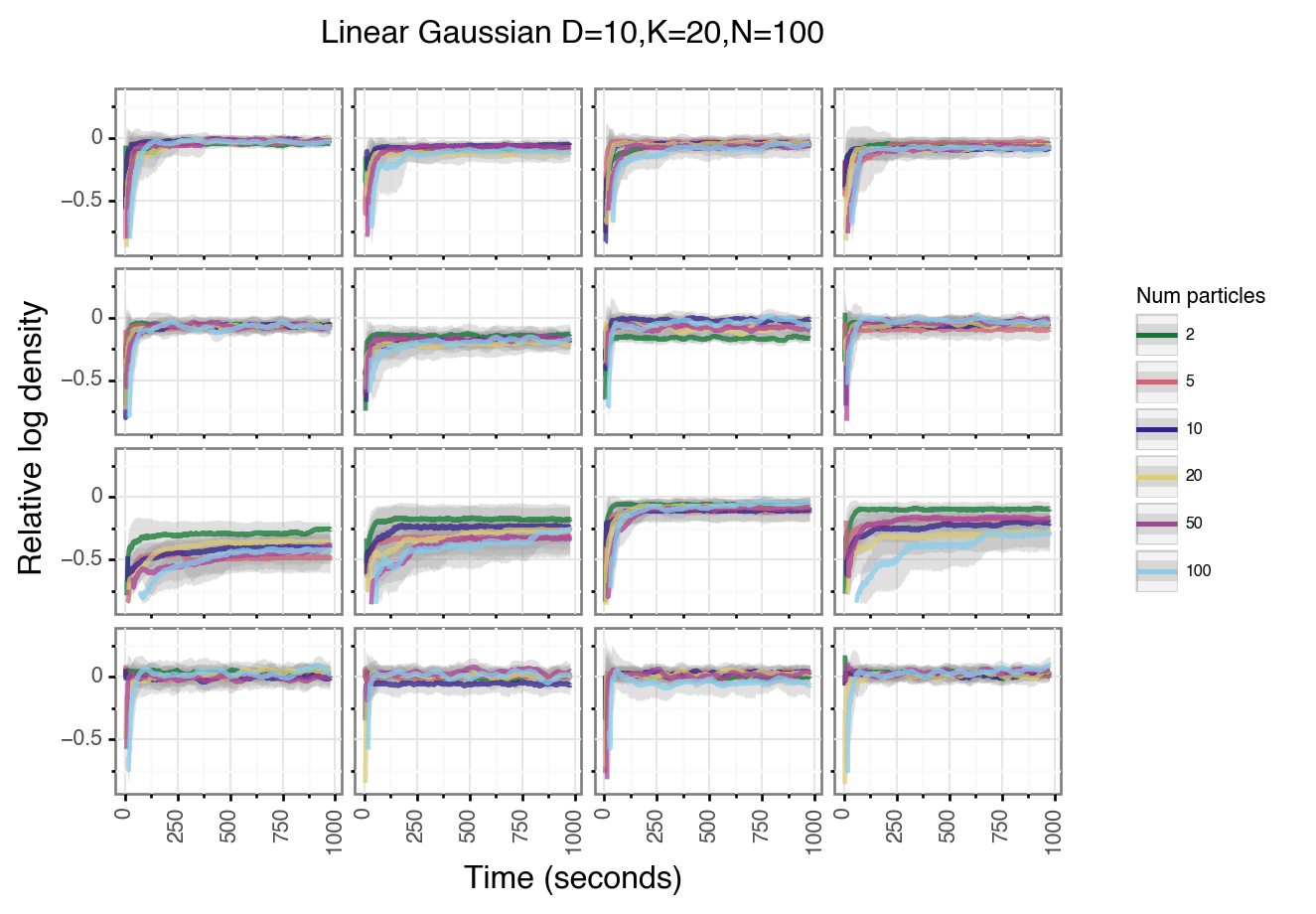
Figure S5: Trace plots of PG sampler using different number of particles. Rows are datasets and columns are initial parameter settings. Error bars are averaged over five restarts of the sampler with different random seeds.

We benchmarked the PG and DPF algorithms using varying number of particles (Figures S5-S7). Both algorithms appear to be relatively insensitive to the number of particles used. Using 50 and 100 particles leads to significantly worse performance for both the PG (Tables LABEL:tab:friedman_pg_num_particles and LABEL:tab:nemenyi_pg_num_particles) and DPF samplers (Tables LABEL:tab:friedman_dpf_num_particles and LABEL:tab:nemenyi_dpf_num_particles) than using fewer particles after the algorithms have run for 10 seconds. However, after 1000 seconds there were no significant differences between the runs with different numbers of particles for either method. One surprising feature is that runs using as few as two particles still work well. We caution this observation may not hold for other models or larger numbers of features, and more particle may be required. We also note that it is possible to parallelize these samplers across particles which would allow for more particles to be used, though we did not investigate this.

3.2.2 Resampling threshold

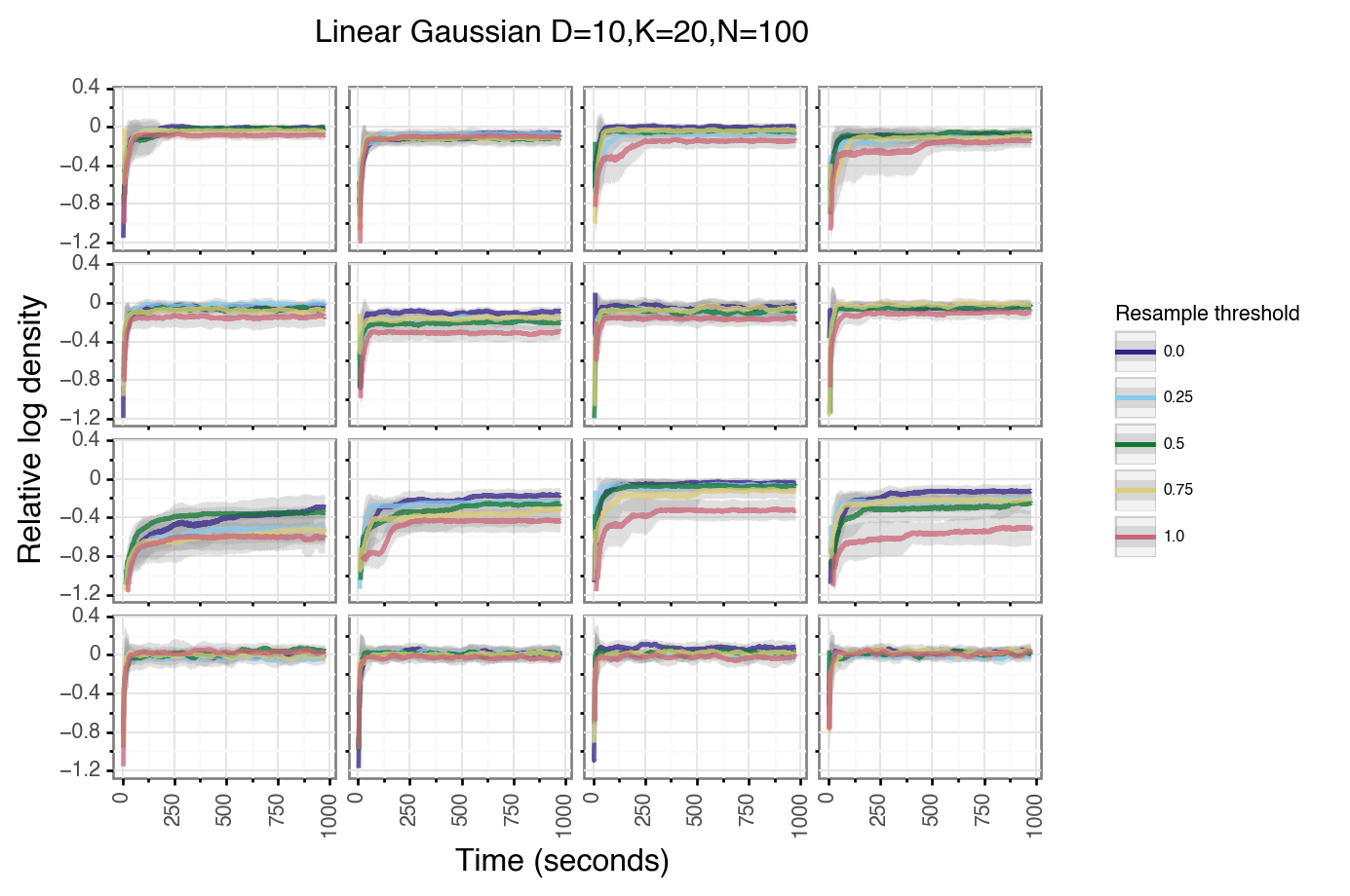
Figure S8: Trace plots of PG sampler using different resampling thresholds. Rows are datasets and columns are initial parameter settings. Error bars are averaged over five restarts of the sampler with different random seeds.

We use an adaptive resampling scheme for the PG algorithm, whereby resampling only occurs if the relative effective sample size (ESS) falls below a specified threshold. The DPF algorithm does not require this tuning parameter as the resampling mechanism is deterministic. Figures S8 and S9 shows the results of the benchmark experiment. The performance of the PG algorithm was insensitive to the value of this parameter with the exception of using a threshold of 1.0 which corresponds to always resampling. Always resampling performed significantly worse (Tables LABEL:tab:friedman_pg_resample_threshold and LABEL:tab:nemenyi_pg_resample_threshold) than several other thresholds at all time points. Somewhat surprisingly when the resampling threshold is 0.0, that is never resampling, the sampler still performed well.

3.2.3 Annealing power

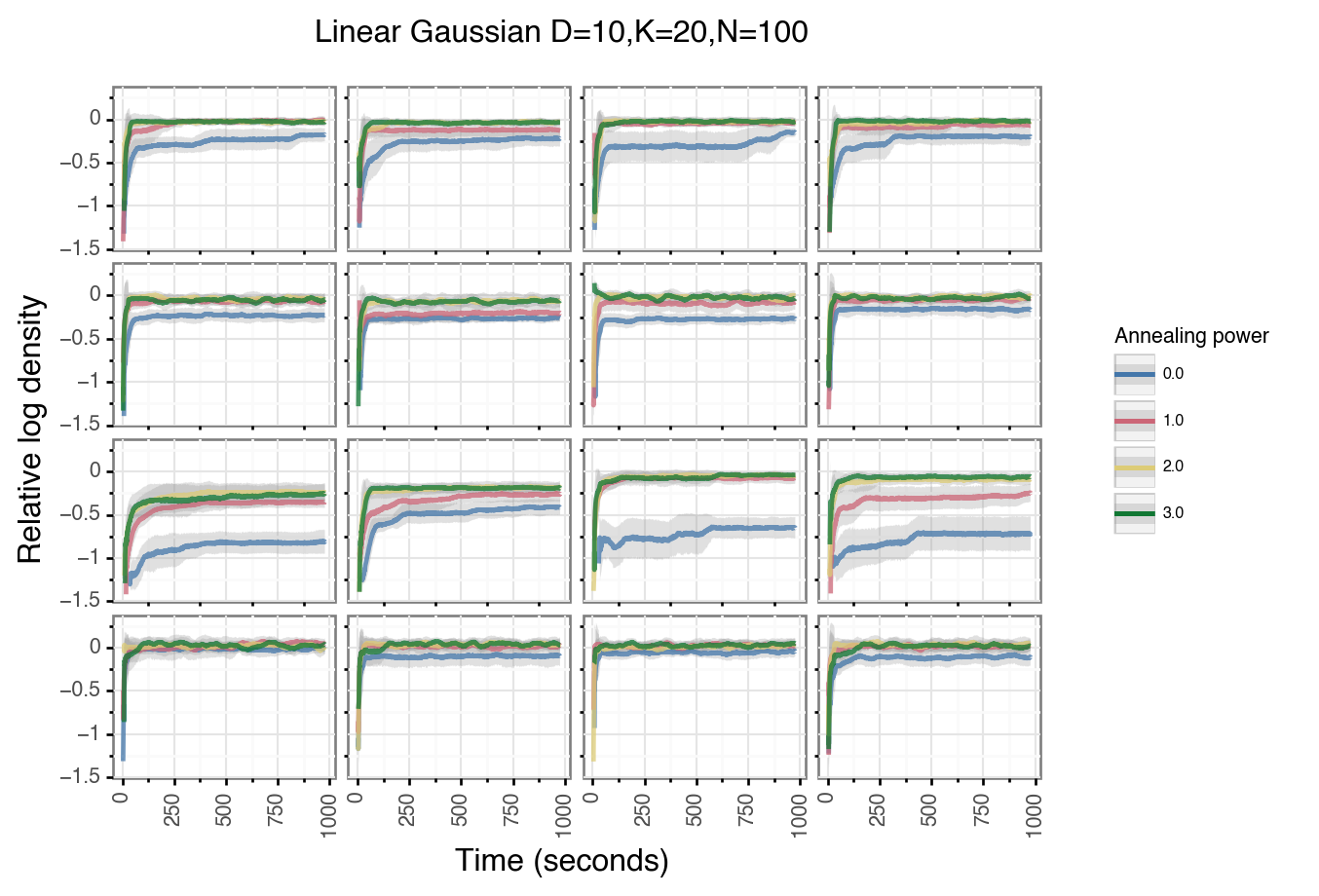
Figure S10: Trace plots of PG sampler using different annealing powers. Rows are datasets and columns are initial parameter settings. Error bars are averaged over five restarts of the sampler with different random seeds.

As discussed in the methods we can use a sequence of target distribution which anneals the data likelihood. In principle this allows the method to defer resampling away particles with low data likelihood at early stages. We explore the impact of the annealing parameter in Figures S10-S12. The PG sampler using no annealing, that is setting the power to zero, performed significantly worse (Tables LABEL:tab:friedman_pg_annealing_power and LABEL:tab:nemenyi_pg_annealing_power). The actual value of the annealing power seemed to be less important provided it was larger than zero. The DPF sampler was generally insensitive to this parameter. The only significant difference observed was between using a power of 0.0 and 3.0 after 10 seconds (Tables LABEL:tab:friedman_dpf_annealing_power and LABEL:tab:nemenyi_dpf_annealing_power) and this difference disappears for later times. This is likely due to the fact all possible paths from early time steps are included in by the DPF sampler, and are not resampled away.

3.2.4 Test path

In order to evaluate the data likelihood term in the target distributions, we must instantiate the values of the feature allocation vector that have not been updated yet. We consider several strategies for doing so:

• Conditional: Use the value of the conditional path.

• Ones: Set the value of all features to one.

• Random: Draw the value of the feature vector uniformly at random.

• Two stage: Run an unconditional SMC sampler using the conditional path to draw a test path.

• Unconditional: Similar to two stage but using zeros as the test path for the first pass unconditional SMC.

• Zeros: Set the value of all features to zero.

The Conditional and Two Stage strategies do not lead to valid Gibbs updates due to the dependency on the conditional path. However, we include them in this analysis as they could be used during a burnin phase. After burnin, another strategy which does lead to a valid Gibbs update could be used. The Two Stage and Unconditional strategies both use a pilot run of unconditional SMC. This increases run time, and introduces additional tuning parameters. For the purpose of this experiment, we set the tuning parameters of both the SMC and cSMC passes to the same values.

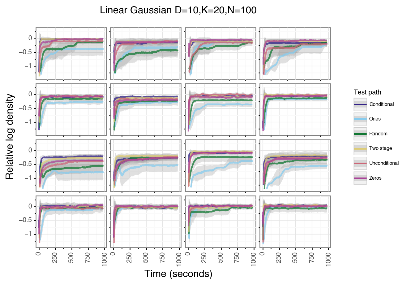
Figure S13: Trace plots of PG sampler using different test paths. Rows are datasets and columns are initial parameter settings. Error bars are averaged over five restarts of the sampler with different random seeds.

Figures S13-S15 show the results of the experiment. For the PG sampler the Ones and Random test paths performed significantly worse than other approaches. At early time points the Conditional and Zeros strategies were the best, but at later time points the Two Stage and Unconstrained approaches were not significantly worse (Tables LABEL:tab:friedman_pg_test_path and LABEL:tab:nemenyi_pg_test_path). For the DPF algorithm the Conditional, Random, and Zeros methods significantly outperformed other approaches after 10 seconds (Tables LABEL:tab:friedman_dpf_test_path and LABEL:tab:nemenyi_dpf_test_path). Both the Conditional and Zeros methods significantly outperformed the Random method at this time. For later time points no methods had significantly different performance. This result suggests that the simple approach of using a test path of zeros is effective, though there may still be some benefit of using the Conditional strategy for burnin. This experiment also suggests that the PG sampler is sensitive to this parameter, whereas the DPF sampler is quite robust.

3.2.5 Summary

Based on these results we used the following parameter values for subsequent experiments.

• Annealing power - 1.0

• Number of particles - 20

• Resample threshold - 0.5

• Test path - Zeros

These were not necessarily the optimal parameters based on the experiments, but were reasonably close to optimal. Note we use the Zeros test path strategy to ensure we have a valid Markov Chain kernel targeting the correct distribution.

3.3 Method comparison

To compare the performance of our proposed approaches to the standard Gibbs sampler we generated synthetic data from three feature allocation models. For all comparisons we ran 80 chains for each sampler as in the tuning experiments. We simulated data with parameter values which should lead to easily identifiable solutions and thus we would expect the samplers to converge to a distribution concentrated on the parameters used for simulation.

3.3.1 Linear Gaussian model

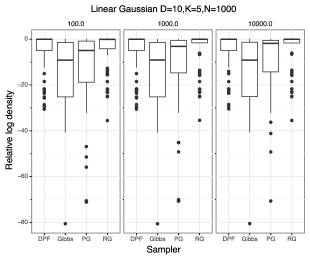
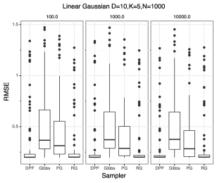
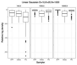
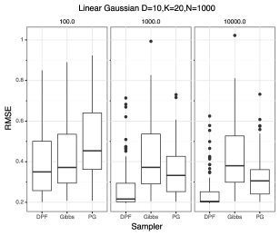
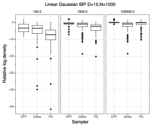
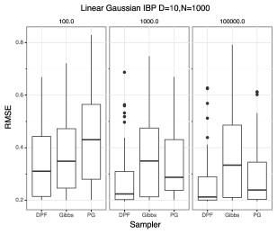
Figure 3: Performance of different samplers using synthetic data from the LG model. The box plots represent the distribution of values from 80 random starts of each parameter setting. We show the values of the relative log density (left, higher is better) and root mean square error reconstruction of missing values (right, lower is better).

We generated datasets using two sets of model parameters. The first dataset was simulated using the FBB prior and $K=5$ and the second was simulated using the FBB model with $K=20$. We fit the second dataset using both the FBB prior with $K=20$ and the IBP prior. For both datasets we simulated $N=1000$ data points from the linear Gaussian model with $\alpha=2$, $\tau_{v}=0.25$, and $\tau_{x}=25$.

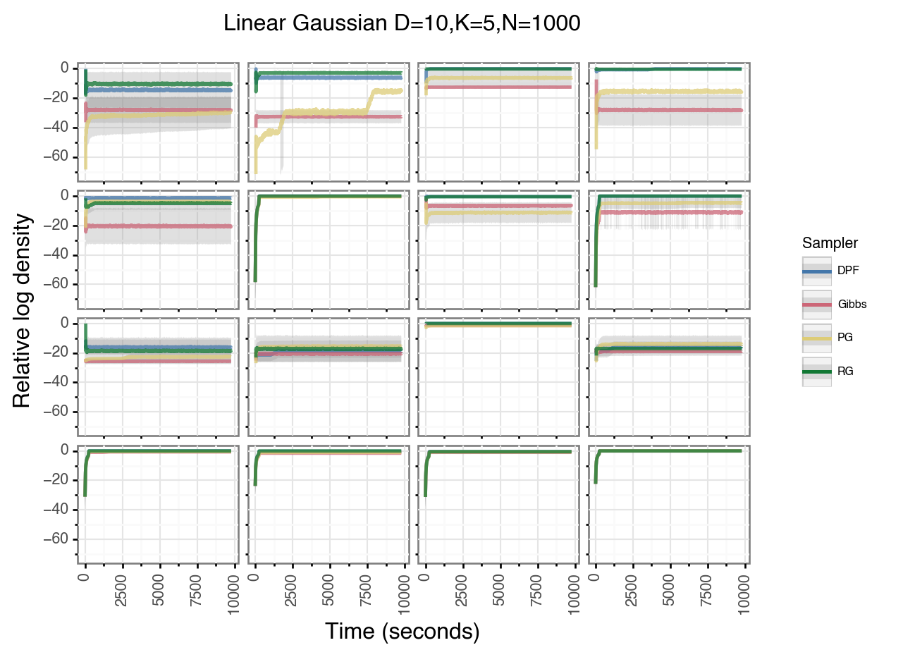
Figure S16: Trace plots of sampling algorithms with simulated data from the linear Gaussian model with K=5. See main text for other model parameters. Rows are datasets and columns are initial parameter settings. Error bars are averaged over five restarts of the sampler with different random seeds.

The results of these experiments are shown in Figure 3 and Figures S16-S18. For the first experiment with $K=5$ it was computationally feasible to use the RG sampler. Because we use 20 particles for the DPF algorithm it is equivalent to the RG sampler in this case. The RG sampler serves as the gold standard for the DPF and PG methods in this experiment. For the $K=5$ dataset the RG sampler significantly outperforms the Gibbs sampler, supporting the results of our initial toy data experiment (Tables LABEL:tab:friedman_lg_finite_5 and LABEL:tab:nemenyi_lg_finite_5). The DPF and RG samplers do not perform significantly different as expected, and outperform the other two approaches. The PG sampler does not significantly outperform the Gibbs sampler.

For the second dataset, fitting the FBB prior model ($K=20$) the DPF sampler does not significantly outperform the Gibbs sampler after 100 seconds (Tables LABEL:tab:friedman_lg_finite_20 and LABEL:tab:nemenyi_lg_finite_20). However, for longer runs the performance advantage of the DPF sampler becomes significant. At the earliest time point the Gibbs sampler significantly outperforms the PG sampler, but the situation reverse at later time points.

The results are somewhat different for the third experiment fitting the IBP model. In this case we see that the Gibbs sampler outperformed the PG sampler at early time points (Tables LABEL:tab:friedman_lg_ibp_20 and LABEL:tab:nemenyi_lg_ibp_20). As the samplers were run longer the PG sampler began to outperform the Gibbs sampler. The DPF sampler outperforms both approaches. One explanation for the better performance of the Gibbs sampler over the PG sampler is that the Gibbs sampler can propose more moves to alter the dimensionality of the model in the same time period. Thus during the burnin phase the Gibbs sampler can more efficiently move the model to the correct number of features which improves performance. However, the fact the DPF sampler outperforms both, suggests that the ability to perform efficient updates on the non-singleton columns dominates this effect.

3.3.2 Latent Feature Relational Model

We next explored performance using the LFRM model described by Miller et al. (2009). As for the LG experiment, we generated datasets using two sets of model parameters. We fit the second dataset using both the FBB prior with $K=20$ and the IBP prior. We again executed 80 runs for all samplers using the same strategy as previous experiments. We simulated $N=100$ data points with parameters $\alpha=2$ and $\tau=0.25$ from the non-symmetric LFRM model. We randomly assigned 5% of the data matrix to be missing. In addition to the relative log density we report the reconstruction error of the model for the entire data matrix, both observed and missing values.

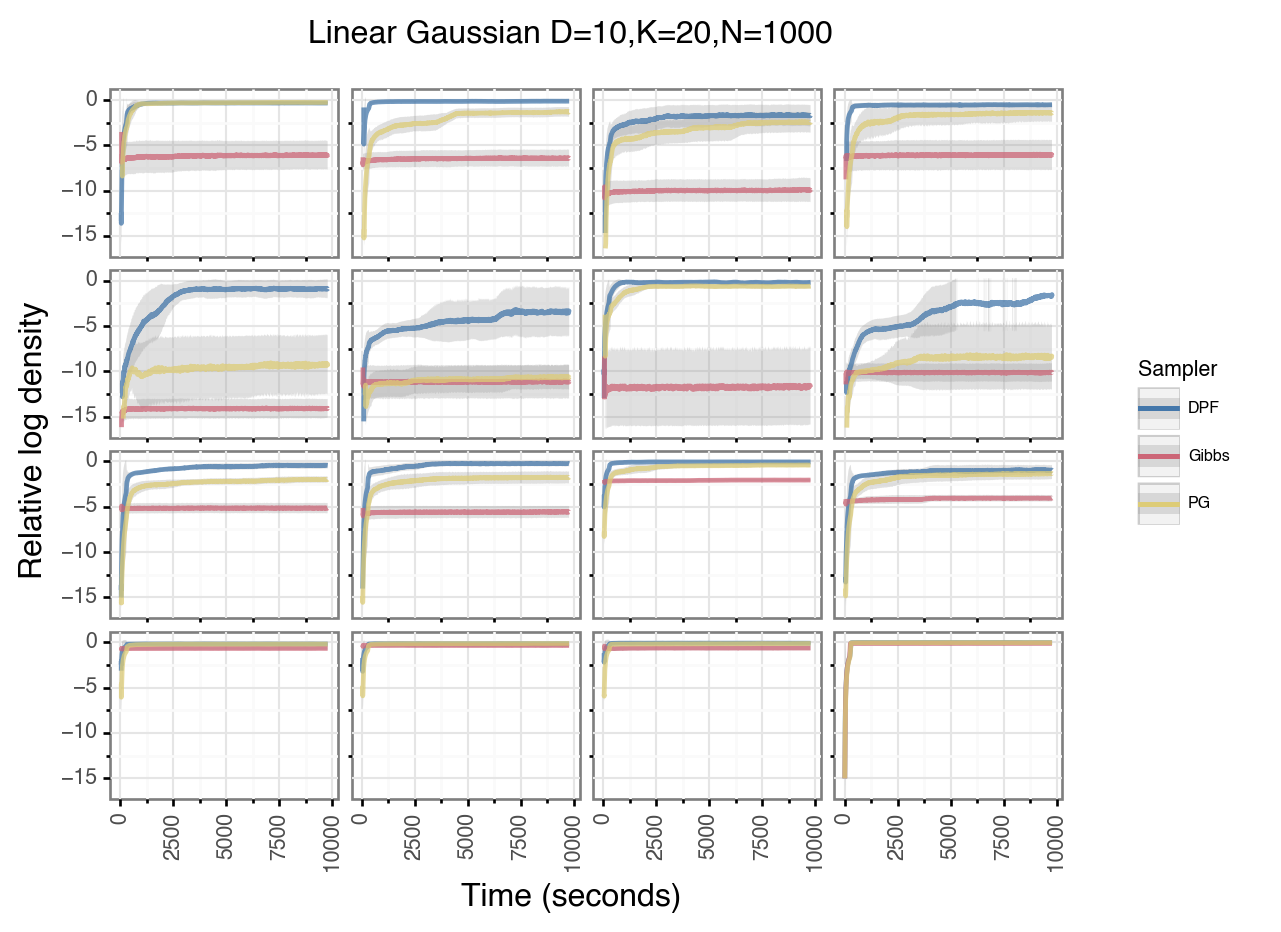
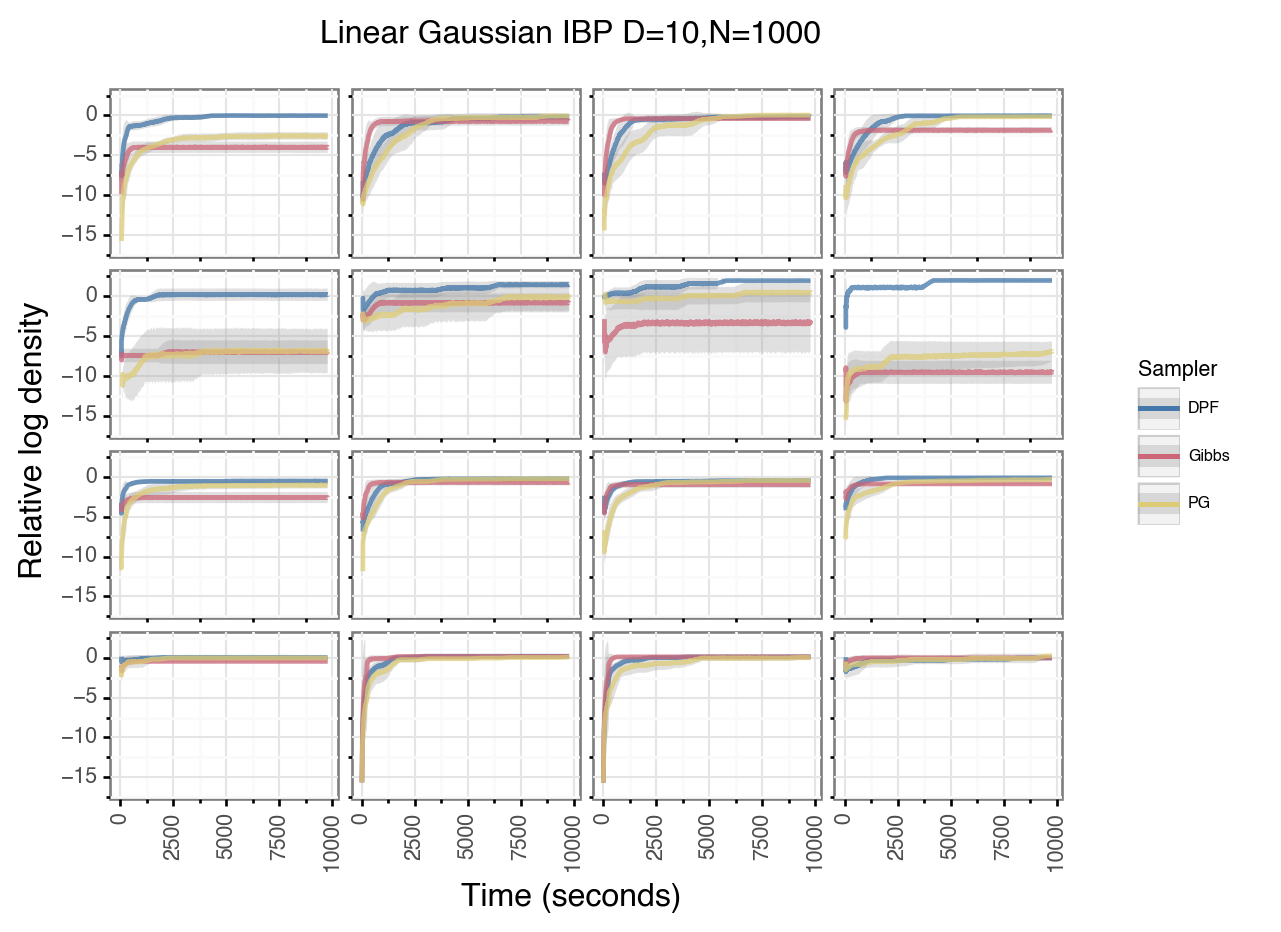
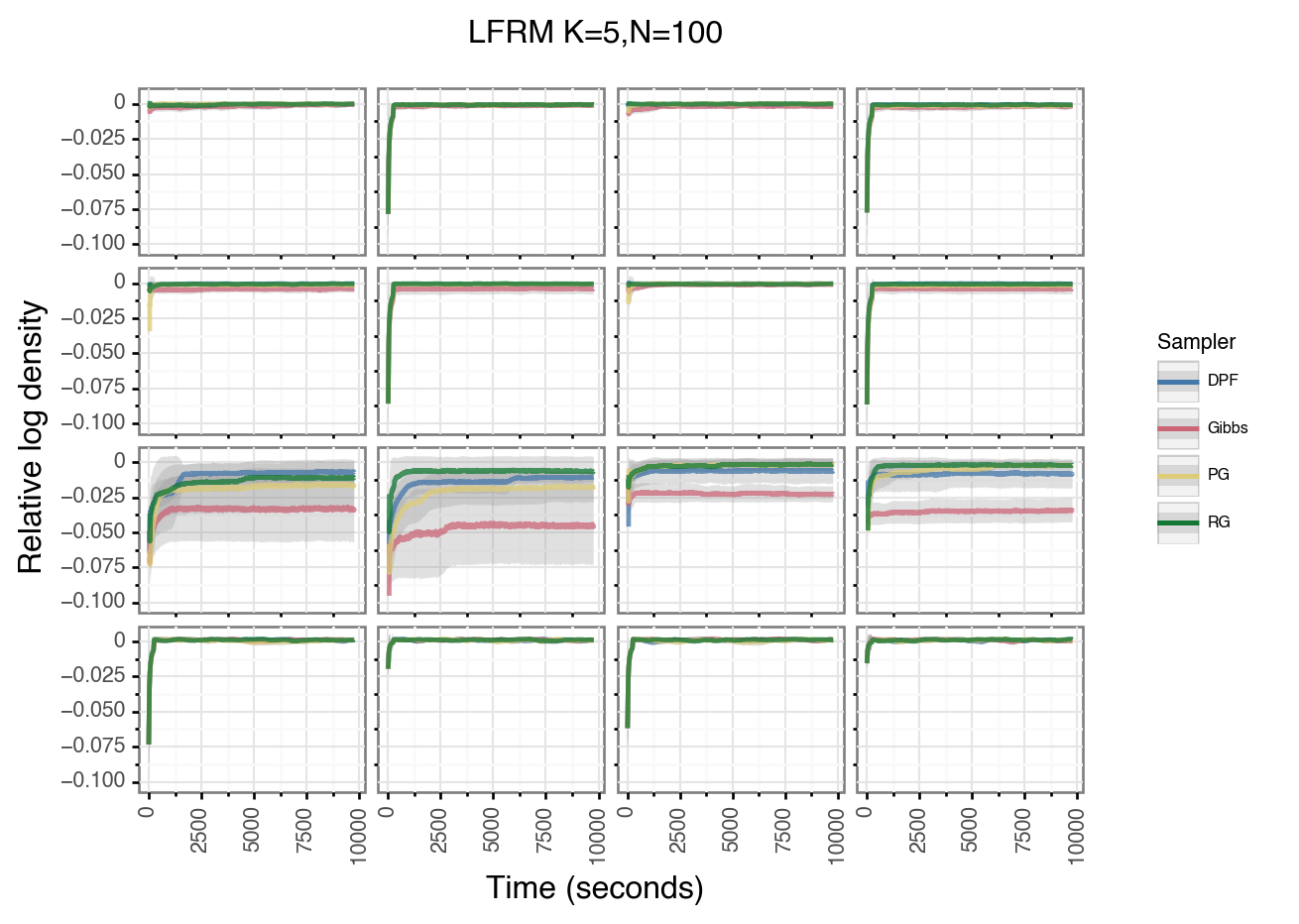
Figure S17: Trace plots of sampling algorithms with simulated data from the linear Gaussian model with K=20. See main text for other model parameters. Rows are datasets and columns are initial parameter settings. Error bars are averaged over five restarts of the sampler with different random seeds.

Figure S18: Trace plots of sampling algorithms with simulated data from the linear Gaussian model with K=20 using an IBP prior. See main text for other model parameters. Rows are datasets and columns are initial parameter settings. Error bars are averaged over five restarts of the sampler with different random seeds.

Figure S19: Trace plots of sampling algorithms with simulated data from the non-symmetric LFRM model with K=5. See main text for other model parameters. Rows are datasets and columns are initial parameter settings. Error bars are averaged over five restarts of the sampler with different random seeds.

The result of these experiments are shown in Figures S19-S22. The RG and DPF methods significantly outperformed the other two methods for the K=5 experiment in terms of relative log density (Tables LABEL:tab:friedman_lfrm_finite_5 and LABEL:tab:nemenyi_lfrm_finite_5). However, the difference in reconstruction error was not significant. There was no significant difference between samplers for the other two runs (Tables LABEL:tab:friedman_lfrm_finite_20-LABEL:tab:nemenyi_lfrm_ibp_20).

3.3.3 PyClone model

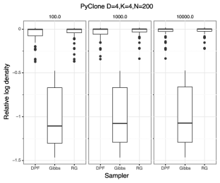
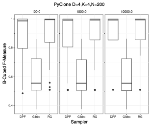
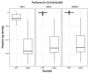
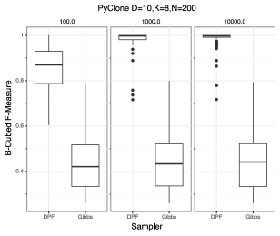
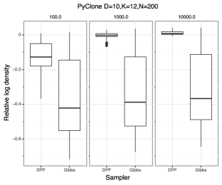
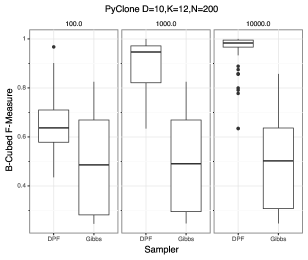
Figure 4: Performance of different samplers using synthetic data from the PyClone model. The box plots represent the distribution of values from 80 random starts of each parameter setting. We show the values of the relative log density (right) and B-Cubed F-measure (left).

The final model we tested with was a modified version of the PyClone model described in Roth et al. (2014). The modifications are described in the supplement. We simulated three datasets using the FBB prior with $\alpha=2$, $a_{V}=b_{V}=1$ with $N=200$ data points. For the first dataset we set $D=4$ and $K=4$, the second we set $D=10$ and $K=8$ and the third $D=10$ and $K=12$. We did not fit the model using the IBP prior as we could not develop an efficient proposal for updating singleton entries. In addition to the relative log density we computed the B-Cubed F-Measure (Amigó et al., 2009). The B-Cubed metric is a measure of feature allocation accuracy analogous to the V-Measure metric (Rosenberg and Hirschberg, 2007) used to evaluate clustering algorithms. We focused on feature allocation accuracy as the features are interpretable quantities that we wish to infer in this application.

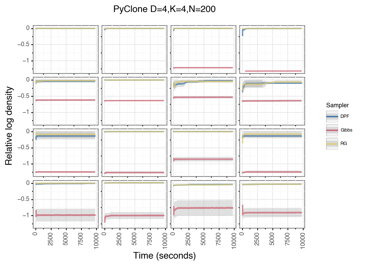
Figure S23: Trace plots of sampling algorithms with simulated data from the PyClone model with D=4 and K=4. See main text for other model parameters. Rows are datasets and columns are initial parameter settings. Error bars are averaged over five restarts of the sampler with different random seeds.

The results of the experiments are shown in Figure 4 and Figures S23-S25. Note that we exclude the PG method from these figures as the performance was so poor as to obscure the scales of the plots. For the first dataset the RG and DPF sampler both outperformed the other approaches (Tables LABEL:tab:friedman_pyclone_finite_4 and LABEL:tab:nemenyi_pyclone_finite_4). The PG approach performed significantly worse than all other approaches including the Gibbs sampler. The two other datasets presented similar trends, with the DPF sampler outperforming both approaches and the PG sampler performing the worst (Tables LABEL:tab:friedman_pyclone_finite_8-LABEL:tab:nemenyi_pyclone_finite_12). The performance of the Gibbs sampler did not improve from times 1000 to 10000. Both the PG and DPF samplers show improved performance as sampling is run for longer. This suggests that the Gibbs sampler is potentially trapped in the vicinity of a local optima, which it cannot escape from.

4 Discussion

In this work we have developed several methods for updating an entire row of a feature allocation matrix. Our results suggest that such samplers can significantly improve performance compared to the widely used single entry Gibbs sampler. Directly implementing row wise Gibbs updates is intractable for more than a small number of features due to the exponential number of feature allocations. We overcome this limitation by using the PG methodology to develop an algorithm which scales linearly in the number of features. When coupled with the DPF framework we obtain significantly better performance than the standard Gibbs sampler. The use of the DPF framework appears to be critical, as the standard PG sampler did not always perform well. In particular, the performance of the PG sampler when applied to the PyClone model was significantly worse than the standard Gibbs sampler. However, the DPF approach significantly outperformed both the Gibbs and PG methods. Furthermore, when applied to models such as the LFRM where the standard Gibbs sampler performs well, our approach does not perform significantly worse. This suggests that despite the increased computational complexity of the PG framework, there is little downside to employing this approach. Taken together our results suggest the DPF algorithm is a computationally efficient and generally applicable approach for performing Bayesian inference for feature allocation models. Our algorithm is applicable to both the parametric FBB and non-parametric IBP model.

We have focused on developing row wise updates for the feature allocation matrix. When applied to the parametric FBB model these updates can significantly improve performance. However, when applied to the non-parametric models using the IBP prior we did not see consistent improvement. We believe a major problem in the non-parametric regime is the updates for the singleton features. The most general approach of using MH updates with proposals from the priors seems to lead to very slow mixing. While this is an issue for the Gibbs sampler as well, the low computational cost of updating non-singleton entries allows this sampler to perform more singleton updates. We believe that the development of efficient schemes to update the columns in a single move will be particularly useful. This has already been explored to some extent in Fox et al. (2014), where split-merge moves are used as proposals for an MH update. It should be possible to further improve upon these split-merge style moves using the PG framework, in a similar way to what has been done in the Bayesian clustering literature (Bouchard-Côté et al., 2017). Such updates would complement the approach we have developed in this work.

We have not exploited the potential for performing parallel computation that is offered by the PG framework. In particular we could parallelize any loops over particles in Algorithm 3 which could potentially yield significant speed-ups. It has been noted by Whiteley et al. (2010) and Lindsten et al. (2014) that the use of backward or ancestor sampling can significantly reduce the effect of path degeneracy for SMC models. These approaches could naturally be combined with our method, and could allow for the use of fewer particles.

5 Appendix

5.1 Models

We describe the three models we used for performance comparisons. We use the notation $Z\mid\alpha\sim\text{FAM}(\cdot\mid\alpha)$ to describe sampling from a feature allocation distribution, either the FBB or IBP priors. The number of features $K$ is implicitly determined by the number of columns of $Z$. We place a $\text{Gamma}(\cdot\mid 1,1)$ prior on the hyper-parameter $\alpha$ and use a random walk Metropolis-Hastings kernel to update the variable.

When referring to the Normal distribution we use the mean/precision parametrization. When referring to the Gamma distribution we use the shape/rate parametrization.

5.1.1 Linear Gaussian

The linear Gaussian model has been widely used, particularly in the IBP literature (see Griffiths and Ghahramani (2011) for example). One reason for the model’s popularity is that it is possible to marginalize the feature parameters, so a collapsed sampler can be developed. In this work we do not exploit this, and instead work with uncollapsed model. The hierarchical model is as follows:

$$Z\mid\alpha \sim \text{FAM}(\cdot\mid\alpha)$$

$$\tau_{v}\mid a_{v},b_{v} \sim \text{Gamma}(\cdot\mid a_{v},b_{v})$$

$$S_{v} = \tau_{v}\,\mathbf{I}_{D}$$

$$\tau_{x}\mid a_{x},b_{x} \sim \text{Gamma}(\cdot\mid a_{x},b_{x})$$

$$S_{x} = \tau_{x}\,\mathbf{I}_{D}$$

$$\boldsymbol{v}_{k}\mid\tau_{v} \sim \text{Normal}(\cdot\mid\mathbf{0},S_{v})$$

$$\boldsymbol{x}_{n}\mid\{\boldsymbol{v}_{k}\}_{k=1}^{K},\tau_{x},\boldsymbol{z}_{n} \sim \text{Normal}(\cdot\mid\sum_{k=1}^{K}z_{nk}\boldsymbol{v}_{k},S_{x})$$

We use a Gibbs kernels to update $\boldsymbol{v}_{k}$, $\tau_{v}$ and $\tau_{x}$. When using the IBP prior we use a collapsed Metropolis-Hastings step to update the singletons (Doshi-Velez and Ghahramani, 2009).

5.1.2 Linear Feature Relational Model

The LFRM model was proposed by Miller et al. (2009). The observed data is a binary matrix $X\in\{0,1\}^{N\times N}$ which encodes interactions between entities. It could for example be used to model relationships on a social network. The model posits that an underlying set of features encoded by $Z$ governs whether the entries in $X$ are on or off. The hierarchical model is as follows:

$$Z\mid\alpha \sim \text{FAM}(\cdot\mid\alpha)$$

$$\tau\mid a,b \sim \text{Gamma}(\cdot\mid a,b)$$

$$v_{kl}\mid\tau \sim \text{Normal}(\cdot|0,\tau)$$

$$x_{ij}\mid\{v_{kl}\},Z \sim \text{Bernoulli}\left(\cdot\mid\sigma\left(\sum_{k=1}^{K}\sum_{l=1}^{K}z_{ik}z_{jl}v_{kl}\right)\right)$$

where $\sigma(x)=\frac{1}{1+e^{-x}}$. Note that the model can be symmetric so that $v_{kl}=v_{lk}$ or non-symmetric by letting these parameters vary independently. We use random walk Metropolis-Hastings kernels to update $\tau$ and $v_{kl}$. When using the IBP prior we use a Metropolis-Hastings kernel with proposals from the prior to update the singletons.

5.2 PyClone

The original PyClone model was proposed by Roth et al. (2014). The model assumes we observe data $a_{nm},b_{nm}\in\mathbb{N}$ which represent the number of sequencing reads without and with mutation $n$ in sample $m$. We refer to $d_{nm}=a_{nm}+b_{nm}$ as the sequencing depth. We refer to the proportion of cells with mutation $n$ in sample $m$, $\phi_{nm}$, as the cellular prevalence. We can model the probability of observing $b_{nm}$ reads with the mutation in the samples by a density $g(b_{nm}\mid d_{nm},\phi_{nm},*)$ where $*$ indicates other quantities which are not relevant to the discussion. In the original PyClone model $\boldsymbol{\phi}_{n}$ is assumed to be sampled from a Dirichlet process so that mutations appearing at similar cellular prevalences are clustered. This corresponds to the biological assumption mutations appear within sub-populations of cells, and that the cellular prevalence is the sum of the proportion of cells in the sub-populations containing the mutation. We can alter this model to explicitly identify which sub-populations have the mutation using a feature allocation model. Let $f_{km}$ be the proportion of cells from population $k$ in sample $m$. We use the feature allocation vector $\boldsymbol{z}_{n}$ for mutation $n$ to encode which sub-populations have the mutation. The cellular prevalence is then given by $\phi_{nm}=\sum_{k=1}^{K}z_{nk}f_{km}$. Substituting this into the observation density $g$ gives the new model. The hierarchical model is as follows:

$$Z\mid\alpha \sim \text{FAM}(\cdot\mid\alpha)$$

$$v_{km}\mid a_{v},b_{v} \sim \text{Gamma}(\cdot\mid a_{v},b_{v})$$

$$f_{km}\mid v_{km} = \frac{v_{km}}{\sum_{l=1}^{K}v_{lm}}$$

$$\phi_{nm}\mid\{f_{km}\}_{k=1}^{K},\boldsymbol{z}_{n} = \sum_{k=1}^{K}z_{nk}f_{km}$$

$$b_{nm}\mid d_{nm},\{f_{km}\}_{k=1}^{K},\boldsymbol{z}_{n},* \sim g(\cdot\mid d_{nm},\phi_{nm},*)$$

Updating $v_{km}$ was somewhat difficult for this model so we used a number of MCMC kernels which included random walk Metropolis-Hastings kernels on either individual $v_{km}$ values or blocks. We also used a Metropolis-Hastings kernel where the proposal was a random permutation of the values for a sample. The final kernel was the Multiple-Try-Metropolis kernel (Liu, 2008).

5.3 Supplementary figures

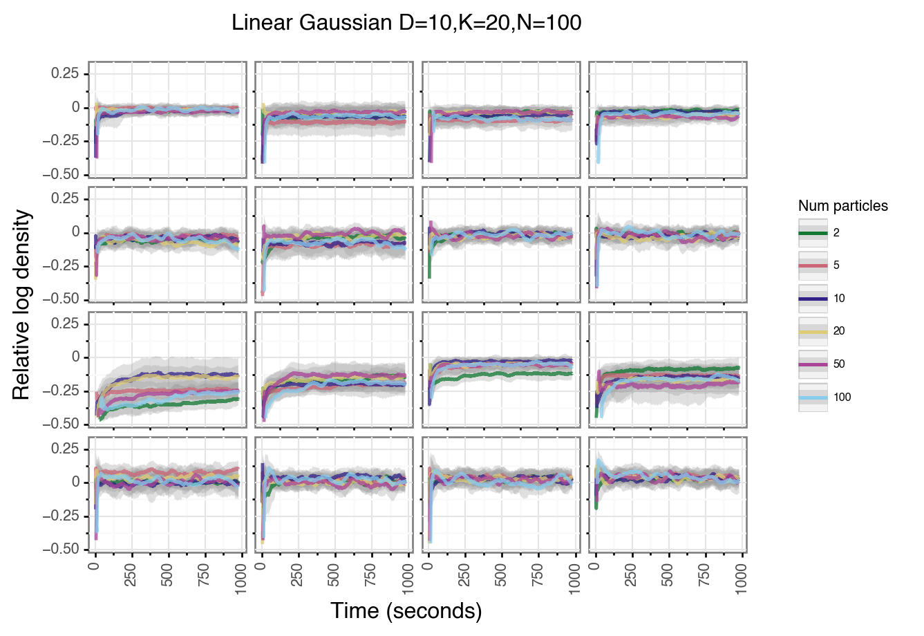
Figure S6: Trace plots of DPF sampler using different number of particles. Rows are datasets and columns are initial parameter settings. Error bars are averaged over five restarts of the sampler with different random seeds.

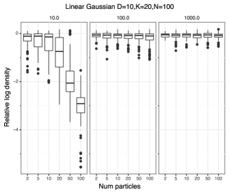
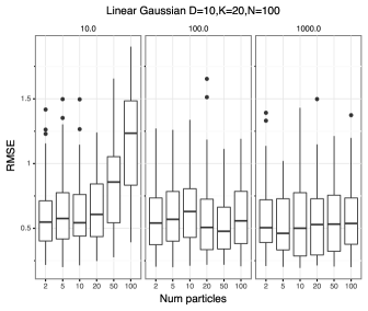
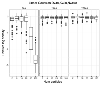
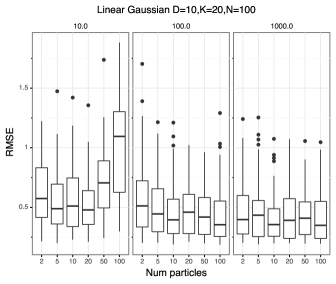
Figure S7: Performance of the PG (top) and DPF (bottom) samplers as function of the number of particles. The box plots represent the distribution of values from 80 random starts of each parameter setting. We show the values of the relative log density (right) and root mean square error reconstruction of missing values (left).

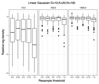
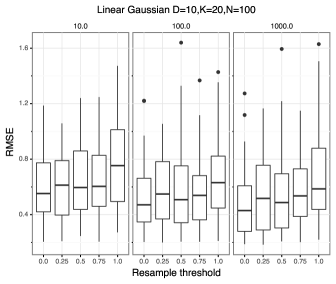
Figure S9: Performance of the PG samplers as function of the resampling threshold. The box plots represent the distribution of values from 80 random starts of each parameter setting. We show the values of the relative log density (right) and root mean square error reconstruction of missing values (left).

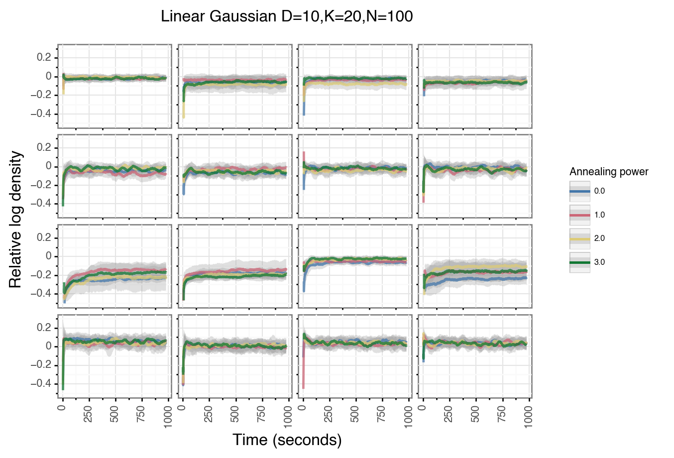
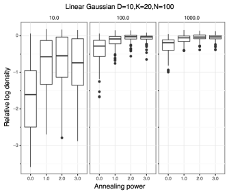
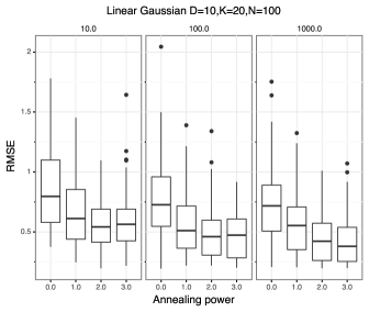
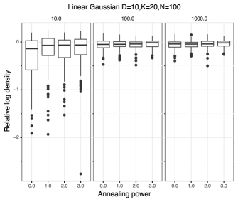
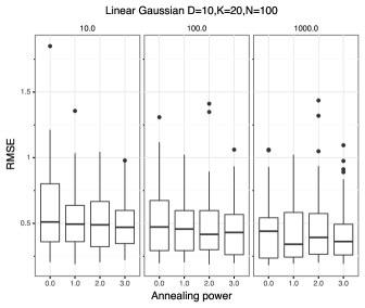
Figure S11: Trace plots of DPF sampler using different annealing powers. Rows are datasets and columns are initial parameter settings. Error bars are averaged over five restarts of the sampler with different random seeds.

Figure S12: Performance of the PG (top) and DPF (bottom) samplers as function of the annealing power of the intermediate target distribution. The box plots represent the distribution of values from 80 random starts of each parameter setting. We show the values of the relative log density (right) and root mean square error reconstruction of missing values (left).

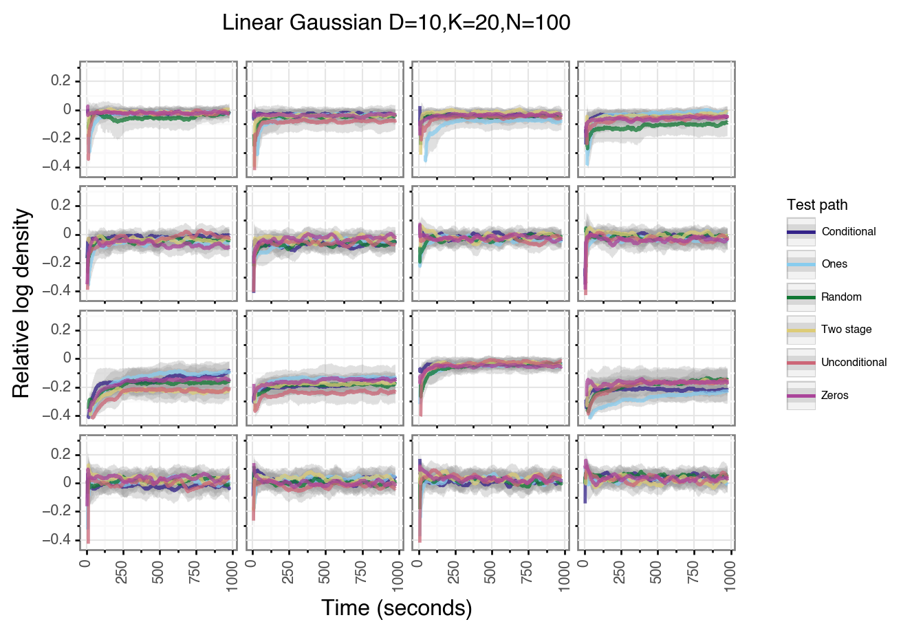
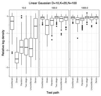
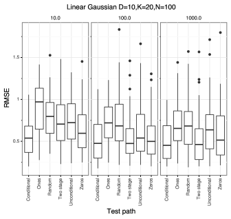
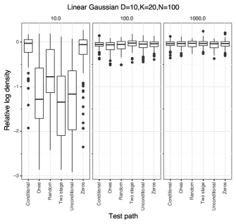
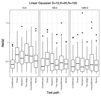
Figure S14: Trace plots of DPF sampler using different test paths. Rows are datasets and columns are initial parameter settings. Error bars are averaged over five restarts of the sampler with different random seeds.

Figure S15: Performance of the PG (top) and DPF (bottom) samplers as function of the test path used to evaluate the data likelihood. The box plots represent the distribution of values from 80 random starts of each parameter setting. We show the values of the relative log density (right) and root mean square error reconstruction of missing values (left).

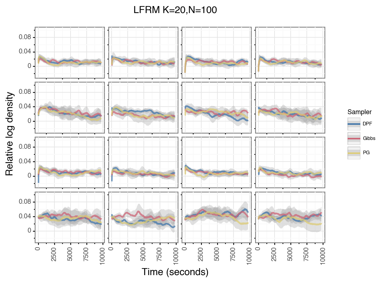
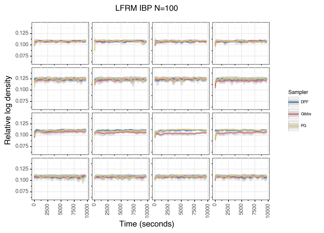
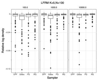
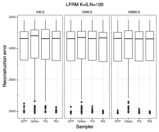
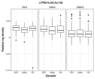
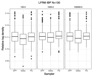
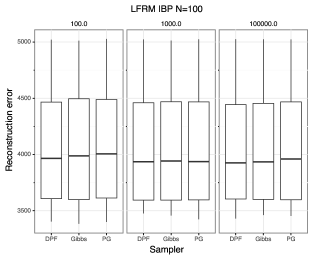
Figure S20: Trace plots of sampling algorithms with simulated data from the non-symmetric LFRM model with K=20. See main text for other model parameters. Rows are datasets and columns are initial parameter settings. Error bars are averaged over five restarts of the sampler with different random seeds.

Figure S21: Trace plots of sampling algorithms with simulated data from the non-symmetric LFRM model with K=20 using an IBP prior. See main text for other model parameters. Rows are datasets and columns are initial parameter settings. Error bars are averaged over five restarts of the sampler with different random seeds.

Figure S22: Performance of different samplers using synthetic data from the LFRM model. The box plots represent the distribution of values from 80 random starts of each parameter setting. We show the values of the relative log density (right) and reconstruction error (left).

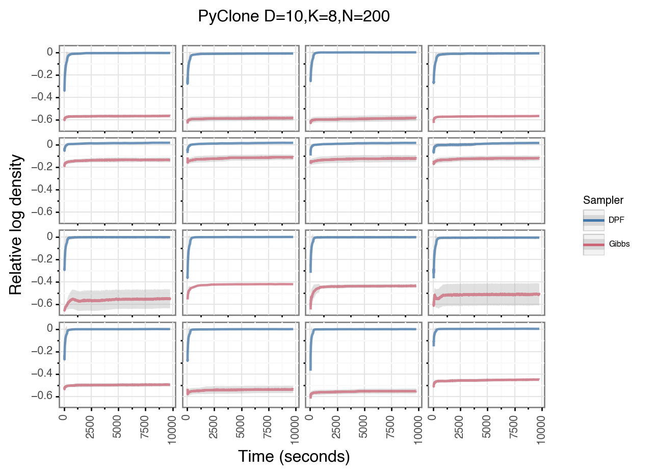
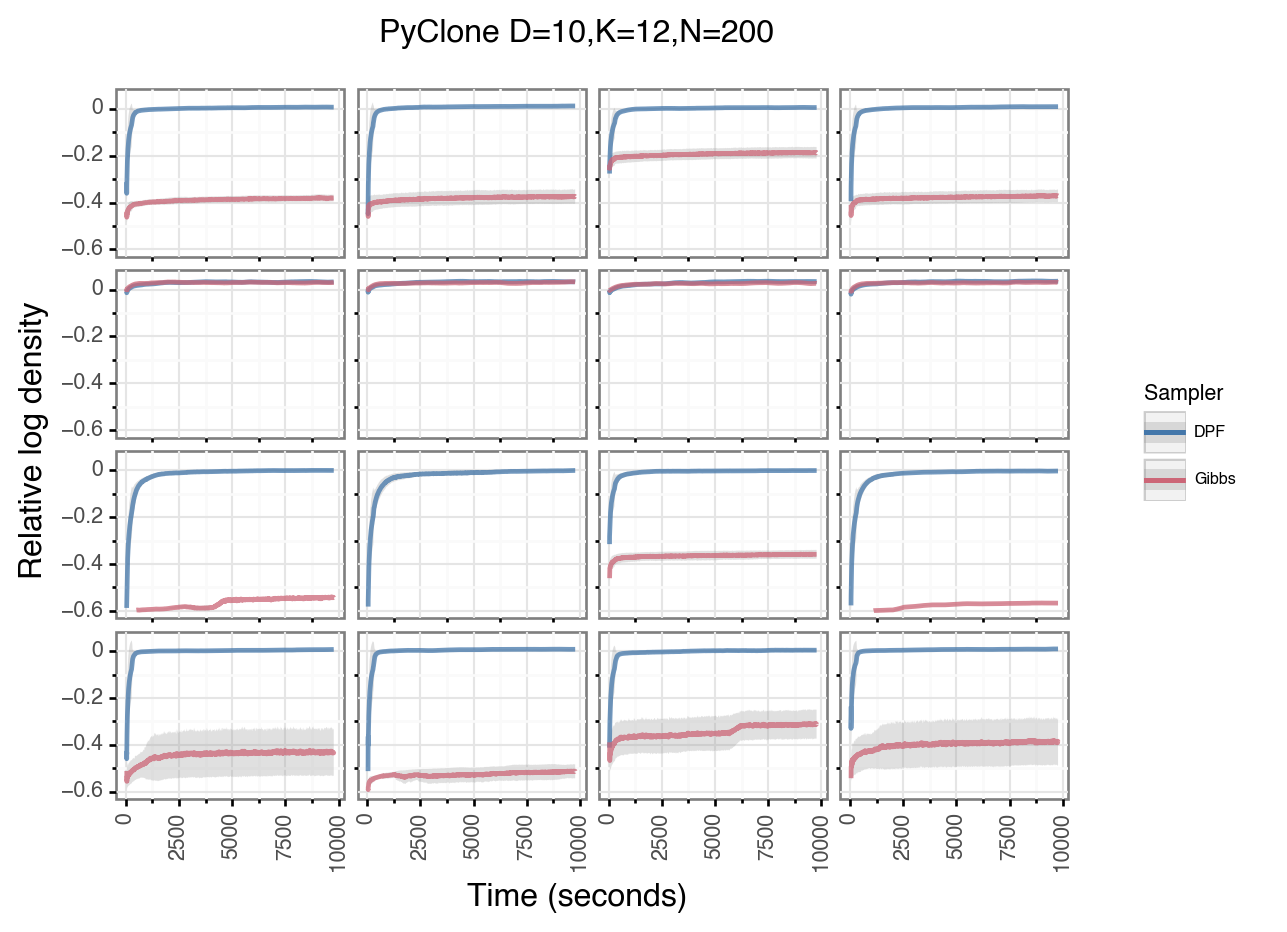
Figure S24: Trace plots of sampling algorithms with simulated data from the PyClone model with D=10 and K=8. See main text for other model parameters. Rows are datasets and columns are initial parameter settings. Error bars are averaged over five restarts of the sampler with different random seeds.

Figure S25: Trace plots of sampling algorithms with simulated data from the PyClone model with D=8 and K=12. See main text for other model parameters. Rows are datasets and columns are initial parameter settings. Error bars are averaged over five restarts of the sampler with different random seeds.

5.4 Supplementary tables

Metric	Relative log density	RMSE
Time
10.0	0.0000	0.0000
100.0	0.0000	0.0060
1000.0	0.0000	0.0393

Table S1: Comparison of the performance of PG algorithm using different number of particles. P-Values are computed using the Friedman test. Significant values at ($p\leq 0.001$) are indicated in bold.

			Relative log density		RMSE
			Mean difference	P-Value	Mean difference	P-Value
Time	Param 1	Param 2
10	10	100	2.7480	0.0000	-0.5587	0.0000
		2	-0.2048	0.5277	0.0359	0.9929
		20	0.3871	0.0245	-0.0349	0.9845
		5	-0.1429	0.6517	-0.0092	1.0000
		50	1.4779	0.0000	-0.2271	0.0001
	100	2	-2.9527	0.0000	0.5946	0.0000
		20	-2.3609	0.0000	0.5238	0.0000
		5	-2.8909	0.0000	0.5495	0.0000
		50	-1.2701	0.0477	0.3316	0.0001
	2	20	0.5918	0.0000	-0.0707	0.7447
		5	0.0619	1.0000	-0.0450	0.9981
		50	1.6826	0.0000	-0.2630	0.0000
	20	5	-0.5300	0.0000	0.0257	0.9640
		50	1.0908	0.0000	-0.1922	0.0031
	5	50	1.6208	0.0000	-0.2179	0.0000
100	10	100	0.1149	0.0477	0.0470	NS
		2	-0.0446	0.3834	0.0728	NS
		20	0.0268	0.9879	0.0589	NS
		5	-0.0005	1.0000	0.0379	NS
		50	0.0207	0.9845	0.1246	NS
	100	2	-0.1595	0.0000	0.0258	NS
		20	-0.0881	0.2976	0.0119	NS
		5	-0.1154	0.0218	-0.0092	NS
		50	-0.0942	0.3180	0.0776	NS
	2	20	0.0713	0.0720	-0.0139	NS
		5	0.0441	0.5526	-0.0350	NS
		50	0.0653	0.0651	0.0518	NS
	20	5	-0.0272	0.9485	-0.0211	NS
		50	-0.0061	1.0000	0.0657	NS
	5	50	0.0212	0.9393	0.0867	NS
1000	10	100	0.0185	0.5776	-0.0345	NS
		2	-0.0104	1.0000	-0.0136	NS
		20	0.0113	0.5776	-0.0082	NS
		5	0.0154	0.9998	0.0311	NS
		50	0.0055	1.0000	-0.0106	NS
	100	2	-0.0289	0.6025	0.0209	NS
		20	-0.0071	1.0000	0.0263	NS
		5	-0.0030	0.8071	0.0656	NS
		50	-0.0129	0.6517	0.0239	NS
	2	20	0.0218	0.6025	0.0054	NS
		5	0.0259	0.9999	0.0447	NS
		50	0.0160	1.0000	0.0030	NS
	20	5	0.0041	0.8071	0.0393	NS
		50	-0.0058	0.6517	-0.0024	NS
	5	50	-0.0099	1.0000	-0.0417	NS

Table S2: Comparison of the performance of PG algorithm using different number of particles. P-Values are computed using the Friedman test. Significant values at ($p\leq 0.001$) are indicated in bold.

Metric	Relative log density	RMSE
Time
10.0	0.0000	0.0000
100.0	0.0000	0.0000
1000.0	0.0000	0.0000

Table S3: Comparison of the performance of DPF algorithm using different number of particles. P-Values are computed using the Friedman test. Significant values at ($p\leq 0.001$) are indicated in bold.

			Relative log density		RMSE
			Mean difference	P-Value	Mean difference	P-Value
Time	Param 1	Param 2
10	10	100	2.4108	0.0000	-0.4485	0.0000
		2	0.0585	0.4064	-0.0628	0.5028
		20	0.0847	1.0000	0.0521	0.9051
		5	-0.0195	1.0000	0.0348	0.9290
		50	1.1853	0.0000	-0.1525	0.0017
	100	2	-2.3523	0.0000	0.3856	0.0000
		20	-2.3261	0.0000	0.5006	0.0000
		5	-2.4303	0.0000	0.4833	0.0000
		50	-1.2254	0.0477	0.2960	0.0001
	2	20	0.0262	0.5776	0.1149	0.0385
		5	-0.0780	0.2976	0.0977	0.0477
		50	1.1269	0.0000	-0.0897	0.3834
	20	5	-0.1042	0.9995	-0.0173	1.0000
		50	1.1007	0.0000	-0.2046	0.0000
	5	50	1.2048	0.0000	-0.1873	0.0000
100	10	100	0.0153	0.7872	0.0301	0.9703
		2	0.0090	0.9947	-0.1183	0.1919
		20	-0.0077	1.0000	-0.0148	0.9998
		5	0.0003	1.0000	-0.0283	1.0000
		50	0.0028	1.0000	0.0044	1.0000
	100	2	-0.0062	0.9879	-0.1484	0.0152
		20	-0.0229	0.7664	-0.0449	0.8609
		5	-0.0149	0.8768	-0.0584	0.9758
		50	-0.0125	0.8440	-0.0256	0.9879
	2	20	-0.0167	0.9929	0.1035	0.3834
		5	-0.0087	0.9991	0.0900	0.1772
		50	-0.0063	0.9981	0.1227	0.1379
	20	5	0.0080	1.0000	-0.0135	0.9997
		50	0.0104	1.0000	0.0193	0.9987
	5	50	0.0024	1.0000	0.0327	1.0000
1000	10	100	0.0307	0.6025	-0.0039	1.0000
		2	-0.0022	0.9995	-0.0688	0.5776
		20	0.0036	1.0000	-0.0359	0.9845
		5	-0.0074	0.9051	-0.0555	0.4539
		50	0.0080	1.0000	-0.0355	0.6025
	100	2	-0.0329	0.3180	-0.0649	0.4299
		20	-0.0271	0.5776	-0.0319	0.9485
		5	-0.0381	0.0588	-0.0516	0.3180
		50	-0.0227	0.6757	-0.0316	0.4539
	2	20	0.0058	0.9997	0.0330	0.9640
		5	-0.0052	0.9906	0.0133	1.0000
		50	0.0102	0.9981	0.0333	1.0000
	20	5	-0.0110	0.9176	-0.0197	0.9176
		50	0.0044	1.0000	0.0003	0.9703
	5	50	0.0153	0.8609	0.0200	1.0000

Table S4: Comparison of the performance of DPF algorithm using different number of particles. P-Values are computed using the Friedman test. Significant values at ($p\leq 0.001$) are indicated in bold.

Metric	Relative log density	RMSE
Time
10.0	0.0000	0.0000
100.0	0.0000	0.0581
1000.0	0.0000	0.0001

Table S5: Comparison of the performance of PG algorithm using different resampling thresholds. P-Values are computed using the Friedman test. Significant values at ($p\leq 0.001$) are indicated in bold.

			Relative log density		RMSE
			Mean difference	P-Value	Mean difference	P-Value
Time	Param 1	Param 2
10	0.0	0.25	-0.0913	0.9846	-0.0222	0.9740
		0.5	-0.0146	1.0000	-0.0581	0.3502
		0.75	-0.0197	1.0000	-0.0552	0.7304
		1.0	0.5900	0.0000	-0.1732	0.0000
	0.25	0.5	0.0767	0.9885	-0.0359	0.8245
		0.75	0.0716	0.9671	-0.0330	0.9885
		1.0	0.6813	0.0000	-0.1510	0.0006
	0.5	0.75	-0.0051	1.0000	0.0029	0.9916
		1.0	0.6047	0.0000	-0.1152	0.0467
	0.75	1.0	0.6097	0.0000	-0.1180	0.0070
100	0.0	0.25	0.0173	0.7797	-0.0516	NS
		0.5	0.0330	0.5100	-0.0577	NS
		0.75	0.0300	0.8643	-0.0361	NS
		1.0	0.1700	0.0000	-0.1385	NS
	0.25	0.5	0.0158	0.9983	-0.0062	NS
		0.75	0.0127	1.0000	0.0155	NS
		1.0	0.1528	0.0001	-0.0869	NS
	0.5	0.75	-0.0030	0.9916	0.0217	NS
		1.0	0.1370	0.0008	-0.0807	NS
	0.75	1.0	0.1400	0.0001	-0.1024	NS
1000	0.0	0.25	0.0507	0.0414	-0.0787	0.2196
		0.5	0.0312	0.4010	-0.0618	0.7797
		0.75	0.0466	0.0664	-0.0985	0.0527
		1.0	0.1380	0.0000	-0.1780	0.0017
	0.25	0.5	-0.0195	0.9134	0.0168	0.9390
		0.75	-0.0041	1.0000	-0.0198	0.9916
		1.0	0.0873	0.0020	-0.0993	0.5947
	0.5	0.75	0.0154	0.9590	-0.0366	0.6505
		1.0	0.1067	0.0000	-0.1161	0.1139
	0.75	1.0	0.0913	0.0010	-0.0795	0.9134

Table S6: Comparison of the performance of PG algorithm using different resampling thresholds. P-Values are computed using the Friedman test. Significant values at ($p\leq 0.001$) are indicated in bold.

Metric	Relative log density	RMSE
Time
10.0	0.0000	0.0000
100.0	0.0000	0.0000
1000.0	0.0000	0.0000

Table S7: Comparison of the performance of PG algorithm using different annealing powers. P-Values are computed using the Friedman test. Significant values at ($p\leq 0.001$) are indicated in bold.

			Relative log density		RMSE
			Mean difference	P-Value	Mean difference	P-Value
Time	Param 1	Param 2
10	0.0	1.0	-0.8443	0.0000	0.1910	0.0051
		2.0	-0.9463	0.0000	0.2878	0.0000
		3.0	-0.8237	0.0000	0.2481	0.0000
	1.0	2.0	-0.1019	0.0703	0.0968	0.0264
		3.0	0.0206	0.9565	0.0571	0.1991
	2.0	3.0	0.1226	0.3172	-0.0397	0.9307
100	0.0	1.0	-0.2557	0.0000	0.1933	0.0003
		2.0	-0.3468	0.0000	0.2685	0.0000
		3.0	-0.3332	0.0000	0.2875	0.0000
	1.0	2.0	-0.0911	0.0020	0.0752	0.5298
		3.0	-0.0775	0.0617	0.0941	0.1448
	2.0	3.0	0.0136	0.8319	0.0189	0.9446
1000	0.0	1.0	-0.1944	0.0000	0.1463	0.0703
		2.0	-0.2415	0.0000	0.2825	0.0000
		3.0	-0.2380	0.0000	0.3128	0.0000
	1.0	2.0	-0.0471	0.1615	0.1362	0.0141
		3.0	-0.0436	0.7219	0.1666	0.0006
	2.0	3.0	0.0034	0.8555	0.0303	0.9148

Table S8: Comparison of the performance of PG algorithm using different annealing powers. P-Values are computed using the Friedman test. Significant values at ($p\leq 0.001$) are indicated in bold.

Metric	Relative log density	RMSE
Time
10.0	0.0000	0.0028
100.0	0.0000	0.0000
1000.0	0.0000	0.0000

Table S9: Comparison of the performance of DPF algorithm using different annealing powers. P-Values are computed using the Friedman test. Significant values at ($p\leq 0.001$) are indicated in bold.

			Relative log density		RMSE
			Mean difference	P-Value	Mean difference	P-Value
Time	Param 1	Param 2
10	0.0	1.0	-0.1168	0.0227	0.0676	NS
		2.0	-0.1317	0.1023	0.0702	NS
		3.0	-0.1392	0.0002	0.0842	NS
	1.0	2.0	-0.0149	0.9820	0.0026	NS
		3.0	-0.0224	0.7219	0.0166	NS
	2.0	3.0	-0.0075	0.3735	0.0140	NS
100	0.0	1.0	-0.0108	0.9996	0.0429	0.9667
		2.0	-0.0034	0.9946	0.0387	0.7514
		3.0	-0.0149	0.9874	0.0622	0.4032
	1.0	2.0	0.0074	0.9751	-0.0043	0.9820
		3.0	-0.0041	0.9982	0.0193	0.8066
	2.0	3.0	-0.0114	0.8970	0.0236	0.9820
1000	0.0	1.0	-0.0076	0.9999	0.0200	0.9999
		2.0	-0.0168	0.6912	-0.0073	0.8319
		3.0	-0.0191	0.9446	0.0342	0.9915
	1.0	2.0	-0.0093	0.7797	-0.0272	0.7514
		3.0	-0.0116	0.9751	0.0142	0.9982
	2.0	3.0	-0.0023	0.9820	0.0415	0.5624

Table S10: Comparison of the performance of DPF algorithm using different annealing powers. P-Values are computed using the Friedman test. Significant values at ($p\leq 0.001$) are indicated in bold.

Metric	Relative log density	RMSE
Time
10.0	0.0000	0.0000
100.0	0.0000	0.0000
1000.0	0.0000	0.0000

Table S11: Comparison of the performance of PG algorithm using different test paths. P-Values are computed using the Friedman test. Significant values at ($p\leq 0.001$) are indicated in bold.

			Relative log density		RMSE
			Mean difference	P-Value	Mean difference	P-Value
Time	Param 1	Param 2
10	Conditional	Ones	1.9441	0.0000	-0.3619	0.0000
		Random	1.2298	0.0000	-0.2472	0.0000
		Two stage	1.2831	0.0000	-0.1914	0.0000
		Unconditional	1.2887	0.0000	-0.2109	0.0000
		Zeros	0.2714	0.4539	-0.0870	0.1055
	Ones	Random	-0.7143	0.0000	0.1147	0.1502
		Two stage	-0.6610	0.0002	0.1705	0.0047
		Unconditional	-0.6554	0.0001	0.1510	0.0062
		Zeros	-1.6727	0.0000	0.2749	0.0000
	Random	Two stage	0.0533	0.9998	0.0558	0.9176
		Unconditional	0.0589	1.0000	0.0362	0.9393
		Zeros	-0.9584	0.0000	0.1602	0.0011
	Two stage	Unconditional	0.0056	1.0000	-0.0195	1.0000
		Zeros	-1.0117	0.0000	0.1044	0.0588
	Unconditional	Zeros	-1.0173	0.0000	0.1239	0.0477
100	Conditional	Ones	0.5421	0.0000	-0.1969	0.0000
		Random	0.2535	0.0000	-0.1982	0.0002
		Two stage	-0.0286	0.3834	0.0011	1.0000
		Unconditional	0.1017	0.1156	-0.1003	0.4064
		Zeros	0.0404	0.9393	-0.0214	0.9845
	Ones	Random	-0.2886	0.0345	-0.0013	0.9998
		Two stage	-0.5707	0.0000	0.1981	0.0000
		Unconditional	-0.4403	0.0000	0.0966	0.0794
		Zeros	-0.5017	0.0000	0.1755	0.0013
	Random	Two stage	-0.2821	0.0000	0.1993	0.0002
		Unconditional	-0.1517	0.0062	0.0979	0.1919
		Zeros	-0.2131	0.0000	0.1768	0.0054
	Two stage	Unconditional	0.1303	0.0001	-0.1015	0.4064
		Zeros	0.0690	0.0308	-0.0226	0.9845
	Unconditional	Zeros	-0.0614	0.6993	0.0789	0.8915
1000	Conditional	Ones	0.1854	0.0000	-0.1978	0.0006
		Random	0.1033	0.0000	-0.2113	0.0001
		Two stage	-0.0091	0.9981	-0.0177	1.0000
		Unconditional	0.0219	0.9929	-0.1663	0.0047
		Zeros	0.0045	1.0000	-0.0879	0.5028
	Ones	Random	-0.0820	0.5028	-0.0135	0.9997
		Two stage	-0.1944	0.0000	0.1801	0.0004
		Unconditional	-0.1634	0.0000	0.0315	0.9987
		Zeros	-0.1808	0.0000	0.1099	0.2411
	Random	Two stage	-0.1124	0.0000	0.1936	0.0001
		Unconditional	-0.0814	0.0004	0.0450	0.9703
		Zeros	-0.0988	0.0000	0.1234	0.0961
	Two stage	Unconditional	0.0310	0.8768	-0.1486	0.0036
		Zeros	0.0136	0.9987	-0.0702	0.4539
	Unconditional	Zeros	-0.0174	0.9906	0.0784	0.5526

Table S12: Comparison of the performance of PG algorithm using different test paths. P-Values are computed using the Friedman test. Significant values at ($p\leq 0.001$) are indicated in bold.

Metric	Relative log density	RMSE
Time
10.0	0.0000	0.0000
100.0	0.0000	0.0000
1000.0	0.0000	0.0000

Table S13: Comparison of the performance of DPF algorithm using different test paths. P-Values are computed using the Friedman test. Significant values at ($p\leq 0.001$) are indicated in bold.

			Relative log density		RMSE
			Mean difference	P-Value	Mean difference	P-Value
Time	Param 1	Param 2
10	Conditional	Ones	1.0392	0.0000	-0.2413	0.0000
		Random	0.6055	0.0000	-0.1644	0.0003
		Two stage	1.2704	0.0000	-0.2645	0.0000
		Unconditional	1.1626	0.0000	-0.2435	0.0000
		Zeros	0.1129	0.9879	-0.0881	0.2239
	Ones	Random	-0.4337	0.0005	0.0769	0.2075
		Two stage	0.2312	0.8261	-0.0232	1.0000
		Unconditional	0.1234	0.9879	-0.0021	0.9987
		Zeros	-0.9263	0.0000	0.1533	0.0003
	Random	Two stage	0.6649	0.0000	-0.1001	0.1772
		Unconditional	0.5571	0.0000	-0.0790	0.5028
		Zeros	-0.4926	0.0000	0.0764	0.4299
	Two stage	Unconditional	-0.1078	0.9972	0.0211	0.9972
		Zeros	-1.1575	0.0000	0.1765	0.0002
	Unconditional	Zeros	-1.0497	0.0000	0.1554	0.0023
100	Conditional	Ones	0.0369	0.7872	-0.1604	0.0001
		Random	0.0150	0.9906	-0.0855	0.7224
		Two stage	-0.0170	0.8071	-0.0123	0.9991
		Unconditional	0.0134	0.9290	-0.0791	0.3609
		Zeros	-0.0023	1.0000	-0.0235	0.8915
	Ones	Random	-0.0219	0.9929	0.0749	0.0308
		Two stage	-0.0539	0.0720	0.1481	0.0006
		Unconditional	-0.0235	0.9999	0.0813	0.1379
		Zeros	-0.0391	0.8768	0.1369	0.0104
	Random	Two stage	-0.0320	0.3391	0.0732	0.9393
		Unconditional	-0.0016	0.9998	0.0064	0.9981
		Zeros	-0.0173	0.9981	0.0620	0.9999
	Two stage	Unconditional	0.0304	0.1633	-0.0668	0.6757
		Zeros	0.0147	0.6993	-0.0112	0.9906
	Unconditional	Zeros	-0.0157	0.9703	0.0556	0.9758
1000	Conditional	Ones	-0.0017	1.0000	-0.0590	0.6993
		Random	0.0009	0.9997	-0.0246	1.0000
		Two stage	-0.0103	0.8261	-0.0273	0.9906
		Unconditional	0.0185	0.9929	-0.0909	0.3609
		Zeros	-0.0075	0.9972	-0.0097	0.9972
	Ones	Random	0.0026	1.0000	0.0344	0.8440
		Two stage	-0.0086	0.9290	0.0317	0.9805
		Unconditional	0.0202	0.9640	-0.0319	0.9987
		Zeros	-0.0059	0.9999	0.0493	0.9567
	Random	Two stage	-0.0112	0.9640	-0.0027	0.9991
		Unconditional	0.0176	0.9290	-0.0663	0.5277
		Zeros	-0.0084	1.0000	0.0149	0.9999
	Two stage	Unconditional	0.0288	0.3834	-0.0637	0.8261
		Zeros	0.0028	0.9879	0.0176	1.0000
	Unconditional	Zeros	-0.0261	0.8609	0.0812	0.7447

Table S14: Comparison of the performance of DPF algorithm using different test paths. P-Values are computed using the Friedman test. Significant values at ($p\leq 0.001$) are indicated in bold.

Metric	Relative log density	RMSE
Time
100.0	0.0000	0.0000
1000.0	0.0000	0.0000
10000.0	0.0000	0.0000

Table S15: Comparison of the performance of sampling algorithm with simulated data from a linear Gaussian model with K=5. See main text for other model parameters. P-Values are computed using the Friedman test. Significant values at ($p\leq 0.001$) are indicated in bold.

			Relative log density		RMSE
			Mean difference	P-Value	Mean difference	P-Value
Time	Sampler 1	Sampler 2
100	DPF	Gibbs	8.7843	0.0000	-0.1836	0.0000
		PG	7.8931	0.0000	-0.1154	0.0000
		RG	-0.2859	0.9999	0.0073	0.9948
	PG	Gibbs	0.8912	0.9736	-0.0683	0.3831
		RG	-8.1790	0.0000	0.1226	0.0000
	RG	Gibbs	9.0702	0.0000	-0.1909	0.0000
1000	DPF	Gibbs	8.7537	0.0000	-0.1851	0.0000
		PG	6.0201	0.0000	-0.0833	0.0000
		RG	-0.4225	0.9614	0.0055	0.6499
	PG	Gibbs	2.7337	0.1589	-0.1018	0.0209
		RG	-6.4425	0.0000	0.0888	0.0000
	RG	Gibbs	9.1762	0.0000	-0.1906	0.0000
10000	DPF	Gibbs	9.0712	0.0000	-0.1974	0.0000
		PG	4.3285	0.0000	-0.0861	0.0000
		RG	-0.0766	0.6499	-0.0145	0.9071
	PG	Gibbs	4.7427	0.1802	-0.1112	0.0209
		RG	-4.4052	0.0000	0.0716	0.0000
	RG	Gibbs	9.1479	0.0000	-0.1829	0.0000

Table S16: Comparison of the performance of sampling algorithm with simulated data from a linear Gaussian model with K=5. See main text for other model parameters. P-Values are computed using the Friedman test. Significant values at ($p\leq 0.001$) are indicated in bold.

Metric	Relative log density	RMSE
Time
100.0	0.0000	0.0000
1000.0	0.0000	0.0000
10000.0	0.0000	0.0000

Table S17: Comparison of the performance of sampling algorithm with simulated data from a linear Gaussian model with K=20. See main text for other model parameters. P-Values are computed using the Friedman test. Significant values at ($p\leq 0.001$) are indicated in bold.

			Relative log density		RMSE
			Mean difference	P-Value	Mean difference	P-Value
Time	Sampler 1	Sampler 2
100	DPF	Gibbs	0.7041	0.0307	-0.0430	0.0246
		PG	8.0163	0.0000	-0.1185	0.0000
	PG	Gibbs	-7.3122	0.0000	0.0754	0.0004
1000	DPF	Gibbs	4.4600	0.0000	-0.1574	0.0000
		PG	1.8011	0.0000	-0.0790	0.0000
	PG	Gibbs	2.6589	0.0000	-0.0784	0.0015
10000	DPF	Gibbs	5.2375	0.0000	-0.1793	0.0000
		PG	1.8331	0.0000	-0.0657	0.0000
	PG	Gibbs	3.4044	0.0000	-0.1136	0.0006

Table S18: Comparison of the performance of sampling algorithm with simulated data from a linear Gaussian model with K=20. See main text for other model parameters. P-Values are computed using the Friedman test. Significant values at ($p\leq 0.001$) are indicated in bold.

Metric	Relative log density	RMSE
Time
100.0	0.0000	0.0000
1000.0	0.0000	0.0000
100000.0	0.0000	0.0000

Table S19: Comparison of the performance of sampling algorithm with simulated data from a linear Gaussian model with K=20 and an IBP prior. See main text for other model parameters. P-Values are computed using the Friedman test. Significant values at ($p\leq 0.001$) are indicated in bold.

			Relative log density		RMSE
			Mean difference	P-Value	Mean difference	P-Value
Time	Sampler 1	Sampler 2
100	DPF	Gibbs	1.7953	0.9695	-0.0275	0.4151
		PG	5.0827	0.0000	-0.0856	0.0000
	PG	Gibbs	-3.2874	0.0000	0.0582	0.0003
1000	DPF	Gibbs	1.5649	0.1180	-0.0974	0.0000
		PG	2.7708	0.0000	-0.0646	0.0000
	PG	Gibbs	-1.2059	0.0000	-0.0328	0.7088
100000	DPF	Gibbs	2.4641	0.0000	-0.1124	0.0000
		PG	1.3703	0.0246	-0.0334	0.0045
	PG	Gibbs	1.0938	0.0000	-0.0790	0.0008

Table S20: Comparison of the performance of sampling algorithm with simulated data from a linear Gaussian model with K=20 and an IBP prior. See main text for other model parameters. P-Values are computed using the Friedman test. Significant values at ($p\leq 0.001$) are indicated in bold.

Metric	Relative log density	Reconstruction error
Time
100.0	0.0000	0.0030
1000.0	0.0000	0.0264
10000.0	0.0000	0.0151

Table S21: Comparison of the performance of sampling algorithm with simulated data from a non-symmetric LFRM model with K=5. See main text for other model parameters. P-Values are computed using the Friedman test. Significant values at ($p\leq 0.001$) are indicated in bold.

			Relative log density		Reconstruction error
			Mean difference	P-Value	Mean difference	P-Value
Time	Sampler 1	Sampler 2
100	DPF	Gibbs	0.0074	0.0002	-40.6125	NS
		PG	0.0038	0.3831	-16.1375	NS
		RG	-0.0006	0.9900	-2.0500	NS
	PG	Gibbs	0.0036	0.0583	-24.4750	NS
		RG	-0.0045	0.2287	14.0875	NS
	RG	Gibbs	0.0081	0.0001	-38.5625	NS
1000	DPF	Gibbs	0.0081	0.0000	-31.5625	NS
		PG	0.0009	0.0681	-5.3125	NS
		RG	-0.0009	0.4940	4.0125	NS
	PG	Gibbs	0.0072	0.0143	-26.2500	NS
		RG	-0.0018	0.7253	9.3250	NS
	RG	Gibbs	0.0091	0.0003	-35.5750	NS
10000	DPF	Gibbs	0.0086	0.0000	-39.3000	NS
		PG	0.0010	0.3831	-9.1125	NS
		RG	-0.0006	0.9071	-9.7125	NS
	PG	Gibbs	0.0076	0.0011	-30.1875	NS
		RG	-0.0016	0.7949	-0.6000	NS
	RG	Gibbs	0.0092	0.0000	-29.5875	NS

Table S22: Comparison of the performance of sampling algorithm with simulated data from a non-symmetric LFRM model with K=5. See main text for other model parameters. P-Values are computed using the Friedman test. Significant values at ($p\leq 0.001$) are indicated in bold.

Metric	Relative log density	Reconstruction error
Time
100.0	0.0004	0.0031
1000.0	0.0031	0.4296
10000.0	0.7886	0.8229

Table S23: Comparison of the performance of sampling algorithm with simulated data from a non-symmetric LFRM model with K=20. See main text for other model parameters. P-Values are computed using the Friedman test. Significant values at ($p\leq 0.001$) are indicated in bold.

			Relative log density		Reconstruction error
			Mean difference	P-Value	Mean difference	P-Value
Time	Sampler 1	Sampler 2
100	DPF	Gibbs	0.0051	0.0011	7.2875	NS
		PG	0.0024	0.9695	-57.6125	NS
	PG	Gibbs	0.0026	0.0026	64.9000	NS
1000	DPF	Gibbs	0.0048	NS	8.7000	NS
		PG	0.0024	NS	-2.8375	NS
	PG	Gibbs	0.0024	NS	11.5375	NS
10000	DPF	Gibbs	-0.0014	NS	0.4000	NS
		PG	0.0015	NS	-1.8875	NS
	PG	Gibbs	-0.0029	NS	2.2875	NS

Table S24: Comparison of the performance of sampling algorithm with simulated data from a non-symmetric LFRM model with K=20. See main text for other model parameters. P-Values are computed using the Friedman test. Significant values at ($p\leq 0.001$) are indicated in bold.

Metric	Relative log density	Reconstruction error
Time
100.0	0.0094	0.0004
1000.0	0.0571	0.4949
100000.0	0.4328	0.6771

Table S25: Comparison of the performance of sampling algorithm with simulated data from a non-symmetric LFRM model with K=20 and an IBP prior. See main text for other model parameters. P-Values are computed using the Friedman test. Significant values at ($p\leq 0.001$) are indicated in bold.

			Relative log density		Reconstruction error
			Mean difference	P-Value	Mean difference	P-Value
Time	Sampler 1	Sampler 2
100	DPF	Gibbs	0.0028	NS	9.3250	0.5345
		PG	0.0007	NS	-16.4625	0.0175
	PG	Gibbs	0.0021	NS	25.7875	0.0004
1000	DPF	Gibbs	0.0013	NS	6.3250	NS
		PG	-0.0010	NS	-3.2625	NS
	PG	Gibbs	0.0023	NS	9.5875	NS
100000	DPF	Gibbs	0.0002	NS	-4.4125	NS
		PG	-0.0004	NS	-6.1000	NS
	PG	Gibbs	0.0006	NS	1.6875	NS

Table S26: Comparison of the performance of sampling algorithm with simulated data from a non-symmetric LFRM model with K=20 and an IBP prior. See main text for other model parameters. P-Values are computed using the Friedman test. Significant values at ($p\leq 0.001$) are indicated in bold.

Metric	Relative log density	B-Cubed F-Measure
Time
100.0	0.0000	0.0000
1000.0	0.0000	0.0000
10000.0	0.0000	0.0000

Table S27: Comparison of the performance of sampling algorithm with simulated data from the PyClone model with D=4 and K=4. See main text for other model parameters. P-Values are computed using the Friedman test. Significant values at ($p\leq 0.001$) are indicated in bold.

			Relative log density		B-Cubed F-Measure
			Mean difference	P-Value	Mean difference	P-Value
Time	Sampler 1	Sampler 2
100	DPF	Gibbs	0.9702	0.0000	0.2967	0.0000
		PG	92.2997	0.0000	0.6791	0.0000
		RG	-0.0144	0.2559	-0.0303	0.4940
	PG	Gibbs	-91.3295	0.0000	-0.3824	0.0000
		RG	-92.3141	0.0000	-0.7093	0.0000
	RG	Gibbs	0.9845	0.0000	0.3270	0.0000
1000	DPF	Gibbs	0.9738	0.0000	0.3128	0.0000
		PG	89.3427	0.0000	0.6741	0.0000
		RG	-0.0116	1.0000	-0.0270	0.9282
	PG	Gibbs	-88.3689	0.0000	-0.3614	0.0000
		RG	-89.3544	0.0000	-0.7012	0.0000
	RG	Gibbs	0.9854	0.0000	0.3398	0.0000
10000	DPF	Gibbs	0.9813	0.0000	0.3402	0.0000
		PG	85.0018	0.0000	0.6797	0.0000
		RG	-0.0084	0.9948	-0.0083	0.9900
	PG	Gibbs	-84.0205	0.0001	-0.3395	0.0000
		RG	-85.0103	0.0000	-0.6879	0.0000
	RG	Gibbs	0.9898	0.0000	0.3484	0.0000

Table S28: Comparison of the performance of sampling algorithm with simulated data from the PyClone model with D=4 and K=4. See main text for other model parameters. P-Values are computed using the Friedman test. Significant values at ($p\leq 0.001$) are indicated in bold.

Metric	Relative log density	B-Cubed F-Measure
Time
100.0	0.0000	0.0000
1000.0	0.0000	0.0000
10000.0	0.0000	0.0000

Table S29: Comparison of the performance of sampling algorithm with simulated data from the PyClone model with D=10 and K=8. See main text for other model parameters. P-Values are computed using the Friedman test. Significant values at ($p\leq 0.001$) are indicated in bold.

			Relative log density		B-Cubed F-Measure
			Mean difference	P-Value	Mean difference	P-Value
Time	Sampler 1	Sampler 2
100	DPF	Gibbs	0.4032	0.0000	0.4152	0.0000
		PG	60.3425	0.0000	0.7977	0.0000
	PG	Gibbs	-59.9393	0.0000	-0.3825	0.2207
1000	DPF	Gibbs	0.4452	0.0000	0.5236	0.0000
		PG	58.3945	0.0000	0.9094	0.0000
	PG	Gibbs	-57.9493	0.0000	-0.3858	0.0568
10000	DPF	Gibbs	0.4391	0.0000	0.5242	0.0000
		PG	53.8505	0.0000	0.8962	0.0000
	PG	Gibbs	-53.4114	0.0000	-0.3719	0.0000

Table S30: Comparison of the performance of sampling algorithm with simulated data from the PyClone model with D=10 and K=8. See main text for other model parameters. P-Values are computed using the Friedman test. Significant values at ($p\leq 0.001$) are indicated in bold.

Metric	Relative log density	B-Cubed F-Measure
Time
100.0	0.0000	0.0000
1000.0	0.0000	0.0000
10000.0	0.0000	0.0000

Table S31: Comparison of the performance of sampling algorithm with simulated data from the PyClone model with D=10 and K=12. See main text for other model parameters. P-Values are computed using the Friedman test. Significant values at ($p\leq 0.001$) are indicated in bold.

			Relative log density		B-Cubed F-Measure
			Mean difference	P-Value	Mean difference	P-Value
Time	Sampler 1	Sampler 2
100	DPF	Gibbs	0.2250	0.0002	0.1678	0.0000
		PG	29.3156	0.0000	0.4260	0.0000
	PG	Gibbs	-29.0906	0.0000	-0.2582	0.8022
1000	DPF	Gibbs	0.3318	0.0015	0.3967	0.0000
		PG	24.7551	0.0000	0.6541	0.0000
	PG	Gibbs	-24.4233	0.0000	-0.2574	0.0002
10000	DPF	Gibbs	0.3240	0.0000	0.4466	0.0000
		PG	13.4891	0.0000	0.5367	0.0000
	PG	Gibbs	-13.1651	0.0000	-0.0902	0.0379

Table S32: Comparison of the performance of sampling algorithm with simulated data from the PyClone model with D=10 and K=12. See main text for other model parameters. P-Values are computed using the Friedman test. Significant values at ($p\leq 0.001$) are indicated in bold.

References

- Amigó et al. (2009) Enrique Amigó, Julio Gonzalo, Javier Artiles, and Felisa Verdejo. A comparison of extrinsic clustering evaluation metrics based on formal constraints. Information retrieval, 12(4):461–486, 2009.
- Andrieu et al. (2010) Christophe Andrieu, Arnaud Doucet, and Roman Holenstein. Particle markov chain monte carlo methods. Journal of the Royal Statistical Society: Series B (Statistical Methodology), 72(3):269–342, 2010.
- Barembruch et al. (2009) Steffen Barembruch, Aurélien Garivier, and Eric Moulines. On approximate maximum-likelihood methods for blind identification: How to cope with the curse of dimensionality. IEEE Transactions on Signal Processing, 57(11):4247–4259, 2009.
- Bouchard-Côté et al. (2017) Alexandre Bouchard-Côté, Arnaud Doucet, and Andrew Roth. Particle gibbs split-merge sampling for bayesian inference in mixture models. The Journal of Machine Learning Research, 18(1):868–906, 2017.
- Broderick et al. (2013) Tamara Broderick, Michael I Jordan, Jim Pitman, et al. Cluster and feature modeling from combinatorial stochastic processes. Statistical Science, 28(3):289–312, 2013.
- Chopin et al. (2015) Nicolas Chopin, Sumeetpal S Singh, et al. On particle gibbs sampling. Bernoulli, 21(3):1855–1883, 2015.
- Demšar (2006) Janez Demšar. Statistical comparisons of classifiers over multiple data sets. Journal of Machine learning research, 7(Jan):1–30, 2006.
- Doshi-Velez and Ghahramani (2009) Finale Doshi-Velez and Zoubin Ghahramani. Accelerated sampling for the indian buffet process. In Proceedings of the 26th annual international conference on machine learning, pages 273–280. ACM, 2009.
- Doucet and Johansen (2009) Arnaud Doucet and Adam M Johansen. A tutorial on particle filtering and smoothing: Fifteen years later. Handbook of nonlinear filtering, 12(656-704):3, 2009.
- Fearnhead and Clifford (2003) Paul Fearnhead and Peter Clifford. On-line inference for hidden markov models via particle filters. Journal of the Royal Statistical Society: Series B (Statistical Methodology), 65(4):887–899, 2003.
- Fox et al. (2014) Emily B Fox, Michael C Hughes, Erik B Sudderth, Michael I Jordan, et al. Joint modeling of multiple time series via the beta process with application to motion capture segmentation. The Annals of Applied Statistics, 8(3):1281–1313, 2014.
- Ghahramani and Griffiths (2006) Zoubin Ghahramani and Thomas L Griffiths. Infinite latent feature models and the indian buffet process. In Advances in neural information processing systems, pages 475–482, 2006.
- Griffiths and Ghahramani (2011) Thomas L Griffiths and Zoubin Ghahramani. The indian buffet process: An introduction and review. Journal of Machine Learning Research, 12(Apr):1185–1224, 2011.
- Lindsten et al. (2014) Fredrik Lindsten, Michael I Jordan, and Thomas B Schön. Particle gibbs with ancestor sampling. The Journal of Machine Learning Research, 15(1):2145–2184, 2014.
- Liu (2008) Jun S Liu. Monte Carlo strategies in scientific computing. Springer Science & Business Media, 2008.
- Meeds et al. (2007) Edward Meeds, Zoubin Ghahramani, Radford M Neal, and Sam T Roweis. Modeling dyadic data with binary latent factors. In Advances in neural information processing systems, pages 977–984, 2007.
- Miller et al. (2009) Kurt Miller, Michael I Jordan, and Thomas L Griffiths. Nonparametric latent feature models for link prediction. In Advances in neural information processing systems, pages 1276–1284, 2009.
- Rosenberg and Hirschberg (2007) Andrew Rosenberg and Julia Hirschberg. V-measure: A conditional entropy-based external cluster evaluation measure. In Proceedings of the 2007 joint conference on empirical methods in natural language processing and computational natural language learning (EMNLP-CoNLL), pages 410–420, 2007.
- Roth et al. (2014) Andrew Roth, Jaswinder Khattra, Damian Yap, Adrian Wan, Emma Laks, Justina Biele, Gavin Ha, Samuel Aparicio, Alexandre Bouchard-Côté, and Sohrab P Shah. Pyclone: statistical inference of clonal population structure in cancer. Nature methods, 11(4):396, 2014.
- Whiteley et al. (2010) Nick Whiteley, Christophe Andrieu, and Arnaud Doucet. Efficient bayesian inference for switching state-space models using discrete particle markov chain monte carlo methods. arXiv preprint arXiv:1011.2437, 2010.
- Wood and Griffiths (2007) Frank Wood and Thomas L Griffiths. Particle filtering for nonparametric bayesian matrix factorization. In Advances in neural information processing systems, pages 1513–1520, 2007.