Properties of $Z_{c}(3900)$ tetraquark in a cold nuclear matter

Abstract

The study of medium effects on properties of particles embedded in nuclear matter is of great importance for understanding the nature and internal quark-gluon organization as well as exact determination of the quantum numbers, especially of the exotic states. In this context, we study the physical properties of one of the famous charmonium-like states, $Z_{c}(3900)$, in a cold dense matter. We investigate the possible shifts in the mass and current-meson coupling of the $Z_{c}(3900)$ state due to the dense medium at saturation density, $\rho^{sat}$, by means of the in-medium sum rules. We also estimate the vector self-energy of this state at saturation nuclear matter density. We discuss the behavior of the spectroscopic parameters of this state with respect to the density up to a high density corresponding to the core of neutron stars, $\rho\approx 5\rho^{sat}$. Both the mass and current-coupling of this state show nonlinear behavior and decrease with respect to the density of the medium: the mass reaches roughly $30\%$ of its vacuum value at $\rho=5\rho^{sat}$, while the current-coupling approaches zero at $\rho\approx 2.1\rho^{sat}$, when the central values of the auxiliary and other input parameters are used.

I Introduction

The standard hadrons are divided into $q\bar{q}$ and $qqq/\bar{q}\bar{q}\bar{q}$ systems. Neither the quark model nor the QCD excludes the existence of the structures out of these configurations. Hence, search for exotic states is inevitable: now we have many exotic states observed in the experiment. We have also made good progress in the determination of different aspects of these states in theory. Most of the discovered exotic states are tetraquarks of the $XYZ$ family. The term $XYZ$ comes from the generalization of states $X(3872)$, $Y(4260)$ and $Z_{c}(3900)$. The $XYZ$ states are the charmonium/bottomonium-like resonances, which, because of their mass, can not be placed in the charmonium/bottomonium picture: These resonances, mainly with $Q\bar{Q}q\bar{q}$ quark content, have different properties than the standard excited quarkonia states. In the last decade, many $XYZ$ states have been observed by the Belle, BESIII, BaBaR, LHCb, CMS, D0, CDF, and CLEO-c collaborations PhysRevD.98.030001 , and their masses, widths and quantum numbers $J^{PC}$ have been predicted. Detailed analysis of the experimental status of these states and various theoretical models can be found in numerous new review articles LIU2019237 ; RevModPhys.90.015004 ; ALI2017123 ; RevModPhys.90.015003 .

In the first trials, the new charmonium-like resonances, discovered in the above experiments, were evaluated as the excited states of ordinary $c\bar{c}$ charmonium states. However, the obtained data showed that some resonances do not conform to standard spectroscopy and thus some new non-conventional models have been developed. The new models differ from each other in terms of their components and strong interaction mechanisms. There are plenty of studies for the physical picture interpretation of the charmonium-like states using the new models: for instance, QCD tetraquark PhysRevD.100.014033 ; Luo2017 , weakly bound hadronic molecules Baru2017 ; CLOSE2004119 ; PhysRevD.76.094028 ; Coito2013 ; PhysRevD.77.034003 ; Cui_2014 ; PhysRevLett.111.132003 , charmonium hybrids ESPOSITO2016292 ; PhysRevLett.54.869 ; Liu2012 ; Li2013 ; PhysRevD.87.116004 , threshold cups PhysRevD.91.094025 ; Swanson:2015bsa ; PAKHLOV2015183 ; PhysRevD.91.051504 and hadro-charmonium DUBYNSKIY2008344 ; Li:2013ssa . Understanding the non-perturbative behaviour of QCD and the strong interaction dynamics that cause the production and structure of these non-conventional states is very important issue for today’s experimental and theoretical studies.

As candidates of tetraquark states, $Z^{\pm}_{c}(3900)$ were reported simultaneously by the BESIII Collaboration PhysRevLett.110.252001 using $e^{+}e^{-}$ annihilation at the vector resonance $Y(4260)$ and by the Belle Collaboration PhysRevLett.110.252002 using the same process but at or near the $\Upsilon(nS)$ ($n=1,\ 2,\ ...,\ 5$) resonances. For the full history see PhysRevLett.95.142001 ; PhysRevD.74.091104 ; PhysRevLett.99.182004 . They were confirmed by the CLEO-c Collaboration using 586 pb^-1 of $e^{+}e^{-}$ annihilation data taken at the CESR collider at $\sqrt{s}=4170$ MeV, the peak of the charmonium resonance $\psi(4160)$. They also reported evidence for $Z_{c}^{0}(3900)$ which is the neutral member of this isospin triplet XIAO2013366 . In Ref. PhysRevLett.112.022001 $e^{+}e^{-}\rightarrow\pi^{\pm}(D\bar{D}^{*})^{\mp}$ at $\sqrt{s}=4.26$ GeV using a 525 pb^-1 data collected at the BEPCII storage ring, the determined pole mass $M_{\textrm{pole}}=(3883.9\pm 1.5$(stat)$\pm 4.2$ (syst)) MeV/$c^{2}$ and pole width $\Gamma_{\textrm{pole}}=(24.8\pm 3.3$(stat)$\pm 11.0$(syst)) MeV were reported with significance of $2\sigma$ and $1\sigma$, respectively. It was referred as $Z_{c}(3885)$. BESIII also observed a new neutral state $Z_{c}(3900)^{0}$ in a process $e^{+}e^{-}\rightarrow\pi^{0}\pi^{0}J/\psi$ with a significance of $10.4\sigma$. The measured mass and width were $(3894.8\pm 2.3$(stat)$\pm 3.2$(syst)) MeV/$c^{2}$ and $\Gamma=(29.6\pm 8.2$(stat)$\pm 8.2$ (syst)) MeV, respectively PhysRevLett.115.112003 . In Ref. PhysRevD.92.092006 , after the full construction of the $D$ meson pair and the bachelor $\pi^{\pm}$ in the final state, the existence of the charged structure $Z^{\pm}_{c}(3885)$ was confirmed in the $(D\bar{D}^{*})^{\mp}$ system and its pole mass and width were measured as $M_{\textrm{pole}}=(3881.7\pm 1.6$(stat)$\pm 1.6$(syst)) MeV/$c^{2}$ and pole width $\Gamma_{\textrm{pole}}=(26.6\pm 2.0$(stat)$\pm 2.1$(syst)) MeV, respectively. In the processes $e^{+}e^{-}\rightarrow D^{+}D^{*-}\pi^{0}+c.c.$ and $e^{+}e^{-}\rightarrow D^{0}\bar{D}^{*0}\pi^{0}+c.c.$ at $\sqrt{s}=4.226$ and $4.257$ GeV the neutral structure $Z_{c}(3885)^{0}$ was observed with the pole mass $(3885.7^{+4.3}_{-5.7}$(stat)$\pm 8.4$ (syst)) MeV/$c^{2}$ and pole width $(35^{+11}_{-12}$(stat)$\pm 15$ (syst)) MeV PhysRevLett.115.222002 . In a very recent study by the D0 Collaboration, the authors presented evidence for the $Z^{\pm}_{c}(3900)$ state decaying to $J/\psi\pi^{\pm}$ in semi-inclusive weak decays of $b-$flavored hadrons PhysRevD.98.052010 .

On theoretical side, for investigation of $Z_{c}(3900)$ resonance, a plenty of different models and approaches are used, some of them are mentioned here as examples. In a recent study Liu:2019gmh , using the three- channel Ross-Shaw theory the authors have obtained constraint conditions that need to be satisfied by various parameters of the theory in order to have a narrow resonance close to the threshold of the third channel, it is relevant to the structure. Using the QCD sum rule method, the same state was considered as a compact tetraquark state of diquark-antidiquark configuration in Kisslinger2015 ; PhysRevD.93.074002 ; PhysRevD.96.034026 and a hadronic molecule in PhysRevD.92.054002 ; PhysRevD.88.014030 . In these studies, many parameters related to the $Z_{c}(3900)$ state were calculated. Its mass was already calculated within the framework of a non-relativistic quark model in Patel2014 , as well.

Despite a lot of theoretical and experimental efforts, unfortunately, the nature and internal structures of most of the exotic states including $Z_{c}(3900)$ are not exactly clear. Hence, investigation of their properties in a dense/hot medium can play an important role. Experiments like PANDA will provide a possibility to explore these states in a dense medium. These studies will help us better understand the quark-gluon organization of the exotic states as well as their interactions with the particles existing in the medium. In our previous study, Ref. AZIZI2018151 , we investigated the $X(3872)$ state by applying a diquark-antidiquark type current in the frame work of in-medium QCD sum rules. We calculated the mass, current-meson coupling and also the vector self-energy of this state and found that these parameters strongly depend on the density of the medium. In the present study, we investigate the effects of a dense medium on the parameters of the $Z_{c}(3900)$ state and look for the behavior of the mass, current-meson coupling and vector self-energy of this charmonium-like state considering it as a compact tetraquark state.

The study is organized as follows. In Sec. II, we derive the spectral densities associated with the state $Z_{c}(3900)$ by applying the two-point sum rule technique and obtain the QCD sum rules for the mass, current-meson coupling and vector self-energy using the obtained spectral densities. In section III, after fixing the auxiliary parameters using the standard prescriptions of the method, the numerical analysis of the physical observables both in vacuum and cold nuclear matter is performed. Section IV is devoted to discussion and concluding remarks. We collect some lengthy expressions obtained from the calculations in the Appendix.

II In-medim mass and current couplings of $Z_{c}(3900)$

Hadrons are formed as a result of some non-perturbative effects at low energies very far from the asymptotic region of QCD. Hence, for investigation of their properties, some non-perturbative methods are needed. QCD sum rule appears as a reliable, powerful and predictive approach in this respect. In this approach, the hadrons are represented by interpolating currents, written considering the quark content and all the quantum numbers of hadrons. From the theoretical studies in vacuum and the experimental data, the quantum numbers $J^{PC}=1^{+-}$ have been assigned to $Z_{c}(3900)$. The comparison of the theoretical predictions on some parameters of this state with the experimental data leads us consider a compact tetraquark of a diquark and an antidiquark structure for this state PhysRevD.93.074002 ; PhysRevD.96.034026 . Thus, the interpolating current representing the $\bar{c}cu\bar{d}$ quark content and $J^{PC}=1^{+-}$ quantum numbers can be written as

$$J_{\mu}(x) = \frac{i\epsilon_{abc}\epsilon_{dec}}{\sqrt{2}}\Bigg{\{}\Big{[}u_{a}^{T}(x)C\gamma_{5}c_{b}(x)\Big{]}\Big{[}\bar{d}_{d}(x)\gamma_{\mu}C\bar{c}^{T}_{e}(x)\Big{]}$$ (1)

$$- \Big{[}u_{a}^{T}(x)C\gamma_{\mu}c_{b}(x)\Big{]}\Big{[}\bar{d}_{d}(x)\gamma_{5}C\bar{c}^{T}_{e}(x)\Big{]}\Bigg{\}},$$

where $\epsilon_{abc}$ and $\epsilon_{dec}$ are anti-symmetric Levi-Civita symbols in three dimensions with color indices $a,b,c,d$ and $e$. The letter $T$ represents a transpose in Dirac space, $\gamma_{5}$ and $\gamma_{\mu}$ are Dirac matrices and $C$ is the charge conjugation operator.

In the framework of QCD sum rule, we aim to obtain the sum rules for the mass, current coupling and vector self-energy of the exotic state $Z_{c}$ in cold nuclear matter. In the generalization of the vacuum QCD sum rules to finite density, we start with the same correlation function of interpolating currents as the vacuum with a difference that, in this case, the time ordering product of the interpolating currents is sandwiched between the ground states of a finite density medium instead of vacuum COHEN1995221 . So, we start with the following in-medium two point correlation function as the building block of the method:

$$\Pi_{\mu\nu}(p)=i\int{d^{4}xe^{ip\cdot x}\langle\psi_{0}|\mathcal{T}[J_{\mu}(x)J^{\dagger}_{\nu}(0)]|\psi_{0}\rangle},$$ (2)

where $p$ is the four momentum of the $Z_{c}$ state, $\mathcal{T}$ is the time ordering operator, and $|\psi_{0}\rangle$ is the parity and time-reversal symmetric ground state of nuclear matter.

In cold nuclear matter, we formulate the sum rules for the modified mass, $m_{Z_{c}}^{*}$, and current coupling constant, $f_{Z_{c}}^{*}$, of the ground state $Z_{c}$. For this purpose and in accordance with the philosophy of the method, the correlation function is calculated in two different perspectives: the phenomenological ($Phe$) and operator product expansion ($OPE$) windows. The results of these two representations are then matched under some conditions like the quark-hadron duality assumption to relate the hadronic parameters to fundamental QCD parameters. We deal with the ground state, hence, we should apply some transformations like the Borel and continuum subtraction to enhance the ground state contribution and suppress the contributions coming from higher states and continuum.

II.1 Phenomenological window

The phenomenological side of the correlation function is determined in a few steps: First, it is saturated by a full set of hadronic states carrying the same numbers as the interpolating current, and then the contribution of the ground state is isolated. As a result, we get

$$\Pi^{Phe}_{\mu\nu}(p)=-\frac{\langle\psi_{0}|J_{\mu}|Z_{c}(p)\rangle\langle Z_{c}(p)|J^{\dagger}_{\nu}|\psi_{0}\rangle}{p^{*2}-m_{Z_{c}}^{*2}}+...,$$ (3)

where $p^{*}$ is the in-medium momentum and dots denote contributions arising from higher resonances and continuum states. The decay constant or current-meson coupling is expressed in terms of the polarization vector $\varepsilon_{\mu}$ of $Z_{c}$ as

$$\langle\psi_{0}|J_{\mu}|Z_{c}(p)\rangle=f^{*}_{Z_{c}}m_{Z_{c}}^{*}\varepsilon_{\mu},$$ (4)

which further simplifies Eq. (3). By summing over the polarization vectors, we can recast the phenomenological side of the correlation function into the form

$$\Pi_{\mu\nu}^{Phe}(p)=-\frac{m^{*2}_{Z_{c}}f^{*2}_{Z_{c}}}{p^{*2}-m^{*2}_{Z_{c}}}\Big{[}-g_{\mu\nu}+\frac{p_{\mu}^{*}p^{*}_{\nu}}{m^{*2}_{Z_{c}}}\Big{]}+....$$ (5)

To proceed, we introduce two self energies: the scalar self-energy $\Sigma_{s}=m^{*}_{Z_{c}}-m_{Z_{c}}$ and the vector self-energy $\Sigma_{\upsilon}$ appears in the expression of the in-medium momentum, $p_{\mu}^{*}=p_{\mu}-\Sigma_{\upsilon}u_{\mu}$ PhysRevC.46.1507 , where $u_{\mu}$ is the four velocity vector of the cold nuclear medium. We work in the rest frame of the medium, i.e. $u_{\mu}=(1,0)$ . As a result, one can write

$$\Pi_{\mu\nu}^{Phe}(p)= - \frac{f^{*2}_{Z_{c}}}{p^{2}-\mu^{2}}\Big{[}-g_{\mu\nu}m^{*2}_{Z_{c}}+p_{\mu}p_{\nu}$$

$$- \Sigma_{\upsilon}p_{\mu}u_{\nu}-\Sigma_{\upsilon}p_{\nu}u_{\mu}+\Sigma_{\upsilon}^{2}u_{\mu}u_{\nu}\Big{]}+...,$$

where $\mu^{2}=m^{*2}_{Z_{c}}-\Sigma^{2}_{\upsilon}+2p_{0}\Sigma_{\upsilon}$, with $p_{0}=p.u$ being the energy of the quasi-particle. The Borel transformed form (Borel with respect to $p^{2}$) of the phenomenological representation reads

$$\Pi_{\mu\nu}^{Phe}(p) = f^{*2}_{Z_{c}}e^{-\mu^{2}/M^{2}}\Big{[}-g_{\mu\nu}m^{*2}_{Z_{c}}$$ (7)

$$+ p_{\mu}p_{\nu}-\Sigma_{\upsilon}p_{\mu}u_{\nu}-\Sigma_{\upsilon}p_{\nu}u_{\mu}+\Sigma_{\upsilon}^{2}u_{\mu}u_{\nu}\Big{]}$$

$$+ ...,$$

where $M^{2}$ is the Borel mass parameter to be fixed later using the standard recipe of the method.

II.2 OPE or QCD window

The QCD side of the calculations can be obtained by inserting the interpolating current $J_{\mu}(x)$ into the correlation function and performing all possible contractions of the quark pairs. The resultant equation is a expression in terms of the in-medium light quark ($S_{q}^{ij}$) and heavy quark ($S_{Q}^{ij}$) propagators:

$$\Pi_{\mu\nu}^{QCD}(p)=-\frac{i}{2}\varepsilon_{abc}\varepsilon_{a^{\prime}b^{\prime}c^{\prime}}\varepsilon_{dec}\varepsilon_{d^{\prime}e^{\prime}c^{\prime}}$$

$$\times \int d^{4}xe^{ipx}\Big{\{}Tr\Big{[}\gamma_{5}\tilde{S}_{u}^{aa^{\prime}}(x)\gamma_{5}S_{c}^{bb^{\prime}}(x)\Big{]}$$

$$\times Tr\Big{[}\gamma_{\mu}\tilde{S}_{c}^{e^{\prime}e}(-x)\gamma_{\nu}S_{d}^{d^{\prime}d}(-x)\Big{]}-Tr\Big{[}[\gamma_{\mu}\tilde{S}_{c}^{e^{\prime}e}(-x)$$

$$\times \gamma_{5}S_{d}^{d^{\prime}d}(-x)\Big{]}Tr\Big{[}\gamma_{\nu}\tilde{S}_{u}^{aa^{\prime}}(x)\gamma_{5}S_{c}^{bb^{\prime}}(x)\Big{]}$$

$$- Tr\Big{[}\gamma_{5}\tilde{S}_{u}^{aa^{\prime}}(x)\gamma_{\mu}S_{c}^{bb^{\prime}}(x)\Big{]}Tr\Big{[}\gamma_{5}\tilde{S}_{c}^{e^{\prime}e}(-x)\gamma_{\nu}S_{d}^{d^{\prime}d}(-x)\Big{]}$$

$$+ Tr\Big{[}\gamma_{\nu}\tilde{S}_{u}^{aa^{\prime}}(x)\gamma_{\mu}S_{c}^{bb^{\prime}}(x)\Big{]}$$

$$\times Tr\Big{[}\gamma_{5}\tilde{S}_{c}^{e^{\prime}e}(-x)\gamma_{5}S_{d}^{d^{\prime}d}(-x)\Big{]}\Big{\}}_{|\psi_{0}\rangle},$$

where $\tilde{S}_{q(c)}=CS_{q(c)}^{T}C$.

The in-medium light and heavy quark propagators in coordinate space in the fixed point gauge and $m_{q}\rightarrow 0$ limit are given as

$$S_{q}^{ij}(x) = \frac{i}{2\pi^{2}}\delta^{ij}\frac{1}{(x^{2})^{2}}\not\!x+\chi^{i}_{q}(x)\bar{\chi}^{j}_{q}(0)$$ (9)

$$- \frac{ig_{s}}{32\pi^{2}}F_{\mu\nu}^{ij}(0)\frac{1}{x^{2}}[\not\!x\sigma^{\mu\nu}+\sigma^{\mu\nu}\not\!x]+\cdots\,,$$

and

$$S_{c}^{ij}(x) = \frac{i}{(2\pi)^{4}}\int d^{4}ke^{-ik\cdot x}\left\{\frac{\delta_{ij}}{\!\not\!{k}-m_{c}}\right.$$

$$\left.-\frac{g_{s}F_{\mu\nu}^{ij}(0)}{4}\frac{\sigma_{\mu\nu}(\!\not\!{k}+m_{c})+(\!\not\!{k}+m_{c})\sigma_{\mu\nu}}{(k^{2}-m_{c}^{2})^{2}}\right.$$

$$\left.+\frac{\pi^{2}}{3}\Big{\langle}\frac{\alpha_{s}GG}{\pi}\Big{\rangle}\delta_{ij}m_{c}\frac{k^{2}+m_{c}\!\not\!{k}}{(k^{2}-m_{c}^{2})^{4}}+\cdots\right\}\,.$$

In the above equations, $\chi^{i}_{q}$ and $\bar{\chi}^{j}_{q}$ are the Grassmann background quark fields and

$$F_{\mu\nu}^{ij}=F_{\mu\nu}^{A}t^{ij,A},~{}~{}~{}~{}~{}A=1,2,...,8,$$ (11)

where $F_{\mu\nu}^{A}$ are classical background gluon fields, and $t^{ij,A}=\frac{\lambda^{ij,A}}{2}$, with $\lambda^{ij,A}$ being the standard Gell-Mann matrices. The next step is to use the expressions of the quark propagators in Eq. (II.2). This leads to two main contributions: perturbative and nonperturbative. The perturbative contributions, which represent the short distance effects are calculated directly by applying the Fourier, Borel and continuum subtraction procedures. The nonperturbative or long distance contributions are expressed in terms of the in-medium quark, gluon and mixed condensates. For the explicit expressions of the condensates and the details of their expansions in terms of different operators see, for instance, Ref. AZIZI2018151 . After insertion of the in-medium condensates in terms of various operators, the Fourier and Borel transformations as well as continuum subtraction are also applied to the nonperturbative part of the QCD side.

The QCD side of the correlation function can be decomposed over the selected Lorentz structures as

$$\Pi_{\mu\nu}^{QCD}(p) = -\Upsilon^{QCD}_{1}(p^{2})g_{\mu\nu}+\Upsilon^{QCD}_{2}(p^{2})p_{\mu}p_{\nu}$$ (12)

$$- \Upsilon^{QCD}_{3}(p^{2})p_{\mu}u_{\nu}-\Upsilon^{QCD}_{4}(p^{2})p_{\nu}u_{\mu}$$

$$+ \Upsilon^{QCD}_{5}(p^{2})u_{\mu}u_{\nu},$$

where the invariant functions $\Upsilon^{QCD}_{i}$ ($i=1,...,5$) in Eq. (12) are given in terms of the following dispersion integrals:

$$\Upsilon^{QCD}_{i}(p^{2})=\int_{4m_{c}^{2}}^{\infty}\frac{\rho_{i}^{QCD}(s)}{s-p^{2}}ds,$$ (13)

where $\rho_{i}^{QCD}(s)$ are the two-point spectral densities related to the imaginary parts of the selected coefficients. The main purpose of the QCD side of the calculations is to calculate these spectral densities. To this end and after insertion of the quark propagators into the correlation function we use the relation

$$\frac{1}{(x^{2})^{m}} = \int\frac{d^{D}k}{(2\pi)^{D}}e^{-ik\cdot x}i(-1)^{m+1}2^{D-2m}\pi^{D/2}$$ (14)

$$\times \frac{\Gamma[D/2-m]}{\Gamma[m]}\Big{(}-\frac{1}{k^{2}}\Big{)}^{D/2-m},$$

to bring $x$ to the exponential. In this way, the resultant expressions contain four four-integrals: one over four-$k$ coming from the above relation one initially existing in the correlation function (integral over four-$x$) and the last two over four-$k_{1}$ and four-$k_{2}$ coming from the heavy quark propagators. The next step is to perform the four integral over $x$, which gives a Dirac delta function. We use this function to perform integral over $k_{1}$. The remaining two integrals over four-$k_{2}$ and four-$k$ are performed using the Feynman parametrization and the formula

$$\int d^{4}\ell\frac{(\ell^{2})^{m}}{(\ell^{2}+\Delta)^{n}}=\frac{i\pi^{2}(-1)^{m-n}\Gamma[m+2]\Gamma[n-m-2]}{\Gamma[2]\Gamma[n](-\Delta)^{n-m-2}}.$$ (15)

Finally, by applying the relation

$$\Gamma\Big{[}\frac{D}{2}-n\Big{]}\Big{(}-\frac{1}{\Delta}\Big{)}^{D/2-n}=\frac{(-1)^{n-1}}{(n-2)!}(-\Delta)^{n-2}ln[-\Delta],$$ (16)

and expansion of $ln[-\Delta]$, we get the imaginary parts of the $\Upsilon^{QCD}_{i}$ functions.

We apply the Borel transformation with respect to the variable $p^{2}$ and perform subtraction procedure according to the standard prescriptions of the method. As a result, we get

$$\mathbf{\Upsilon}^{QCD}_{i}(M^{2},s_{0}^{*})=\int_{4m_{c}^{2}}^{s^{*}_{0}}ds\rho^{QCD}_{i}(s)e^{-\frac{s}{M^{2}}},$$ (17)

where $s_{0}^{*}$ is the in-medium continuum threshold parameter separating the contributions of the ground state $Z_{c}$ and higher resonances and continuum. It will be fixed later. The spectral density related to each structure is the sum of the spectral densities of the perturbative (pert), two-quark ($qq$), two-gluon ($gg$) and mixed quark-gluon ($qgq$) parts:

$$\rho_{i}^{QCD}(s) = \rho_{i}^{pert}(s)+\rho_{i}^{qq}(s)+\rho_{i}^{gg}(s)+\rho_{i}^{qgq}(s).$$ (18)

As an example, for the $g_{\mu\nu}$ structure, these spectral densities are collected in the Appendix.

To obtain the QCD sum rules for the mass, current coupling constant and vector self energy of the $Z_{c}$ state, the coefficients of the same structures from both the $\Pi_{i}^{Phe}$ and $\Pi_{i}^{QCD}$ functions are equated. We get the following sum rules for the physical quantities under consideration:

$$-m^{*2}_{Z_{c}}f^{*2}_{Z_{c}}e^{-\frac{\mu^{2}}{M^{2}}} = \mathbf{\Upsilon}^{QCD}_{1}(M^{2},s_{0}^{*}),$$

$$f^{*2}_{Z_{c}}e^{-\frac{\mu^{2}}{M^{2}}} = \mathbf{\Upsilon}^{QCD}_{2}(M^{2},s_{0}^{*}),$$

$$-\Sigma_{\upsilon}f^{*2}_{Z_{c}}e^{-\frac{\mu^{2}}{M^{2}}} = \mathbf{\Upsilon}^{QCD}_{3}(M^{2},s_{0}^{*}),$$

$$-\Sigma_{\upsilon}f^{*2}_{Z_{c}}e^{-\frac{\mu^{2}}{M^{2}}} = \mathbf{\Upsilon}^{QCD}_{4}(M^{2},s_{0}^{*}),$$

$$\Sigma^{2}_{\upsilon}f^{*2}_{Z_{c}}e^{-\frac{\mu^{2}}{M^{2}}} = \mathbf{\Upsilon}^{QCD}_{5}(M^{2},s_{0}^{*}).$$ (19)

III Numerical Results

In this section, the QCD sum rules presented in Eq. (II.2) are used to investigate the behavior of the mass, current-meson coupling and vector self energy of $Z_{c}$ state in cold nuclear matter. To this end we need the values of some input parameters and in-medium condensates entering the expressions of the obtained sum rules. The in-medium expectation values of different operators together with some other input parameters used in the calculations are: $\rho^{sat}=0.11^{3}~{}$GeV³, $p_{0}=3887.2\pm 2.3$ MeV PhysRevD.98.030001 , $\langle q^{{\dagger}}q\rangle_{\rho}=\frac{3}{2}\rho$, $\langle\bar{q}q\rangle_{0}=(-0.241)^{3}$ GeV³ IOFFE2006232 , $\langle\bar{q}q\rangle_{\rho}=\langle\bar{q}q\rangle_{0}+\frac{\sigma_{\pi N}}{2m_{q}}\rho$ PhysRevC.47.2882 , $m_{q}=\frac{m_{u}+m_{d}}{2}=0.00345$ GeV PhysRevD.98.030001 , $\langle\frac{\alpha_{s}}{\pi}G^{2}\rangle_{0}=(0.33\pm 0.04)^{4}~{}$GeV⁴, $\langle\frac{\alpha_{s}}{\pi}G^{2}\rangle_{\rho}=\langle\frac{\alpha_{s}}{\pi}G^{2}\rangle_{0}-(0.65\pm 0.15)~{}$GeV$~{}\rho$, $\langle q^{{\dagger}}iD_{0}q\rangle_{\rho}=0.18~{}$GeV$~{}\rho$, $\langle\bar{q}iD_{0}q\rangle_{\rho}=0$, $\langle q^{{\dagger}}iD_{0}iD_{0}q\rangle_{\rho_{N}}=0.031~{}GeV^{2}~{}\rho_{N}-\frac{1}{12}\langle q^{{\dagger}}g_{s}\sigma Gq\rangle_{\rho_{N}}$, $\langle\bar{q}g_{s}\sigma Gq\rangle_{0}=m_{0}^{2}\langle\bar{q}q\rangle_{0}$ COHEN1995221 , $m_{0}^{2}=0.8~{}$GeV² IOFFE2006232 , $\langle\bar{q}g_{s}\sigma Gq\rangle_{\rho}=\langle\bar{q}g_{s}\sigma Gq\rangle_{0}+3~{}GeV^{2}~{}\rho$,$\langle q^{{\dagger}}g_{s}\sigma Gq\rangle_{\rho}=-0.33~{}GeV^{2}~{}\rho$, $\langle q^{{\dagger}}iD_{0}iD_{0}q\rangle_{\rho}=0.031~{}$GeV${}^{2}~{}\rho-\frac{1}{12}\langle q^{{\dagger}}g_{s}\sigma Gq\rangle_{\rho}$ COHEN1995221 ; PhysRevC.47.2882 . The pion-nucleon sigma term $\sigma_{\pi N}=0.045$ GeV PhysRevD.87.074503 is used. The quark masses are taken as $m_{u}=2.16_{-0.26}^{+0.49}$ MeV, $m_{d}=4.67_{-0.17}^{+0.48}$ MeV and $m_{c}=1.27\pm 0.02$ GeV PhysRevD.98.030001 .

Besides these inputs, the sum rules in Eqs. (II.2) require fixing of two auxiliary parameters: Borel mass parameter $M^{2}$ and the in-medium continuum threshold $s^{*}_{0}$. To proceed, we need to determine their working regions, such that the in-medium mass, current coupling the the vector self energy show mild variations with respect to the changes in these parameters. The upper and lower limits for $M^{2}$ is determined via imposing some conditions according to the standard prescriptions of the method (for details in the case of doubly heavy baryons, see, for instance, Refs. PhysRevD.99.074012 ; PhysRevD.100.074004 ). The working window for $s^{*}_{0}$ is obtained such that the maximum possible pole contribution is obtained and the physical observables show weak dependence on the auxiliary parameters. These requirements lead to the working windows for auxiliary parameters displayed in Table (1).

$M^{2}$	[3 - 5] GeV2
$s^{*}_{0}$	$[17.6-19.4]$ GeV2

Table 1: Working windows for $M^{2}$ and $s^{*}_{0}$.

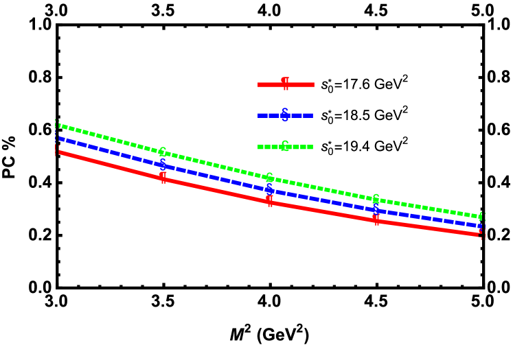
Figure 1: The pole contribution in the $Z_{c}$ channel as a function of $M^{2}$ at saturation nuclear matter density and different fixed values of the in-medium continuum threshold.

As is seen from Fig. (1), the average pole contribution changes in the interval $[57\%-23\%]$ corresponding to $M^{2}=[3-5]$ GeV², which is reasonable in the case of tetraquarks. Our analyses show that the OPE series of sum rules converge very nicely within the working windows of the auxiliary parameters.

Prior to the investigation of the behavior of the in-medium physical quantities, we would like to extract the vacuum mass value for $Z_{c}$ state. The in medium sum rules in the limit $\rho\rightarrow 0$ lead to the average value of vacuum mass as $(3932^{+103}_{-84})$ MeV. We compare this value with the experimental data and other theoretical predictions in vacuum in Table (2). As is seen, our prediction for the vacuum mass of $Z_{c}$ obtained via in-medium sum rules in $\rho\rightarrow 0$ limit is consistent with other presented results within the errors arising mainly from the choice of the auxiliary parameters $M^{2}$ and $s_{0}^{*}$. Note that for Ref. PILLONI2017200 , we presented only one of the results obtained via different scenarios. This result is the closest result to the average experimental value.

	Method	$m_{Z_{c}}$
PS	IMQCDSR ($\rho\rightarrow 0$)	$(3932^{+103}_{-84})$ MeV
PhysRevD.98.030001	Experiment	$(3887.2\pm 2.3)$ MeV
Cui_2014	QCDSR	$(3.88\pm 0.17)$ GeV
PhysRevD.89.054019	QCDSR	$(3.91^{+0.11}_{-0.09})$ GeV
Wang2014	QCDSR	$(3.89^{+0.09}_{-0.09})$ GeV
PILLONI2017200	AAD	$(3893.2^{+5.5}_{-7.7})$ MeV
PhysRevD.96.034026	QCDSR	$(3901^{+125}_{-148})$ MeV
PhysRevD.87.116004	QCDSR	$(3.86\pm 0.27)$ GeV

Table 2: Experimental result and theoretical predictions of different methods for the vacuum mass of $Z_{c}$ state. PS means present study, AAD means amplitude analysis of the data and IMQCDSR refers to the in-medium QCD sum rules.

Now, we proceed to display the behavior of physical quantities under consideration, with respect to the Borel mass and continuum threshold parameters at saturation nuclear matter density, $\rho^{sat}=0.11^{3}$ GeV³. In this respect, we plot the ratio of the in-medium mass to vacuum mass, $m_{Z_{c}}^{*}/m_{Z_{c}}$, and the ratio of the in-medium current meson coupling to its vacuum value, $f_{Z_{c}}^{*}/f_{Z_{c}}$, in Fig. (2). As it is clearly seen, the physical quantities show elegant stability against the changes in the parameters $M^{2}$ and $s_{0}^{*}$ in their working regions. At the saturation nuclear matter density the in-medium mass of $Z_{c}$ state decreases to approximately $77\%$ of its vacuum mass and the shift in average current coupling value of the state due to nuclear medium is about $15\%$.

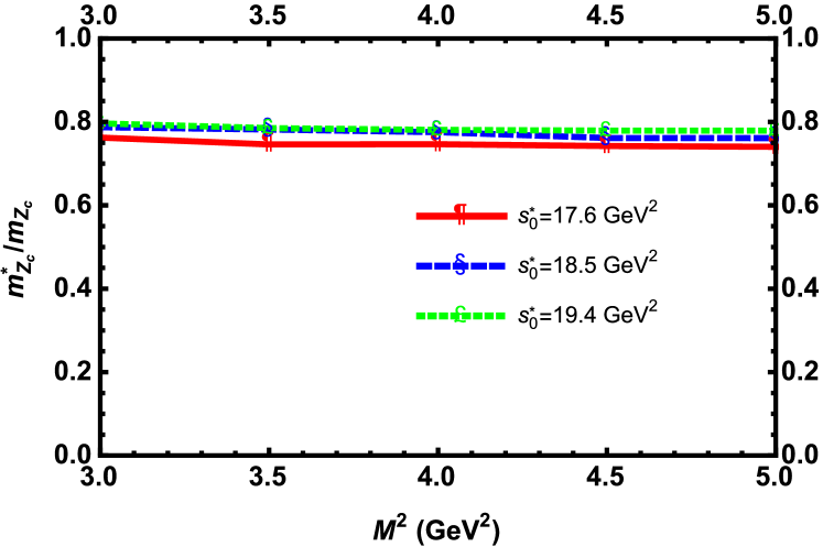
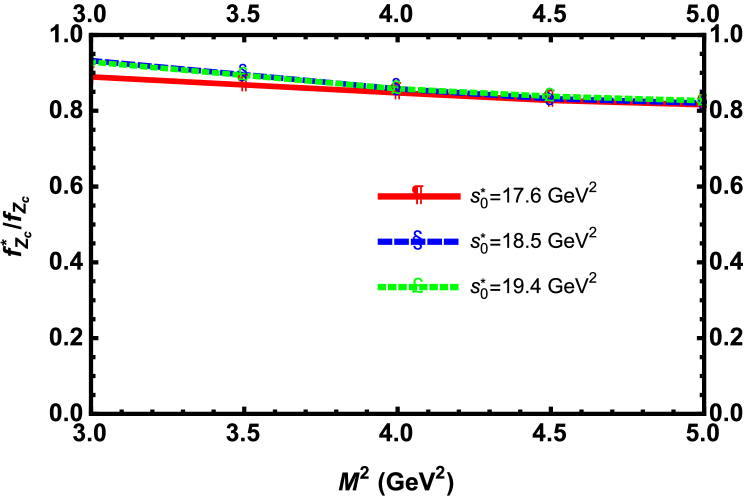
Figure 2: The ratios $m_{Z_{c}}^{*}/m_{Z_{c}}$ and $f_{Z_{c}}^{*}/f_{Z_{c}}$ as functions of $M^{2}$ at the saturated nuclear matter density, $\rho^{sat}=0.11^{3}$ GeV³ and at fixed values of the continuum threshold.

In Fig. (3), the quantities $m_{Z_{c}}^{*}/m_{Z_{c}}$ and $\Sigma_{\nu}/m_{Z_{c}}$ with respect to $M^{2}$ at the average value of continuum threshold and saturation nuclear matter density are shown. As already mentioned, the average negative shift in the modified mass of $Z_{c}$ state due to cold nuclear matter (scalar self energy) is about $23\%$ of the vacuum mass, whereas the vector self-energy, $\Sigma_{\nu}$, is obtained to be approximately $32\%$ of the vacuum value.

Figure 3: The ratios $m_{Z_{c}}^{*}/m_{Z_{c}}$ and $\Sigma_{\nu}/m_{Z_{c}}$ as functions of $M^{2}$ at average value of the continuum threshold and at saturation nuclear matter density.

The main objective in the present study is to investigate the variations of the physical quantities with respect to density of the nuclear medium. To this end, we plot Fig. (4), displaying $m_{Z_{c}}^{*}/m_{Z_{c}}$ and $f_{Z_{c}}^{*}/f_{Z_{c}}$ as functions of $\rho/\rho^{sat}$ at average values of the continuum threshold and Borel parameter. The saturation nuclear matter mass density is $\rho^{sat}=2.7\times 10^{14}$ g/cm³, which is equivalent to $\rho^{sat}=0.16$ fm^-3. However, we need to know the behavior of hadrons at higher densities, which will be accessible in heavy ion collision experiments. Neutron stars as natural laboratories are very compact and dense that may produce hyperons and even heavy baryons and exotic states based on the processes that may occur inside them. For a neutron star with mass $\sim 1.5M_{\odot}$ the relevant core density is approximately ($2\rho^{sat}-3\rho^{sat}$) and for the mass $\sim 2M_{\odot}$ the same density is about $5\rho^{sat}$ Kim:2016yem . Therefore, we would like to discuss the behavior of the mass and coupling constants up to densities comparable with the densities of the neutron stars. However, as it is clear from Fig. (4), the in-medium sum rules give reliable results up to $\rho/\rho^{sat}=1$ and $\rho/\rho^{sat}=1.1$ for $m_{Z_{c}}^{*}/m_{Z_{c}}$ and $f_{Z_{c}}^{*}/f_{Z_{c}}$, respectively. Hence, we need to extrapolate the results to include the higher densities. Our analyses show that the following fit functions well describe the ratios under consideration when the central values of the auxiliary and other input parameters are used:

$$m_{Z_{c}}^{*}/m_{Z_{c}}=e^{-0.252x},$$ (20)

and

$$f_{Z_{c}}^{*}/f_{Z_{c}}=-0.251x^{2}+0.054x+1.028,$$ (21)

where $x=\rho/\rho^{sat}$. From Fig. (4), we see that the fit results coincide with the sum rules predictions at lower densities. The results show that the mass exponentially decreases with respect to $x$ and reaches to roughly $30\%$ of the vacuum mass at a density $5\rho^{sat}$. The coupling constant, however, rapidly changes with respect to $x$ and goes to zero at $x=2.1$. This point may be considered as a pseudocritical density, at which hadrons are melted.

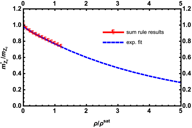
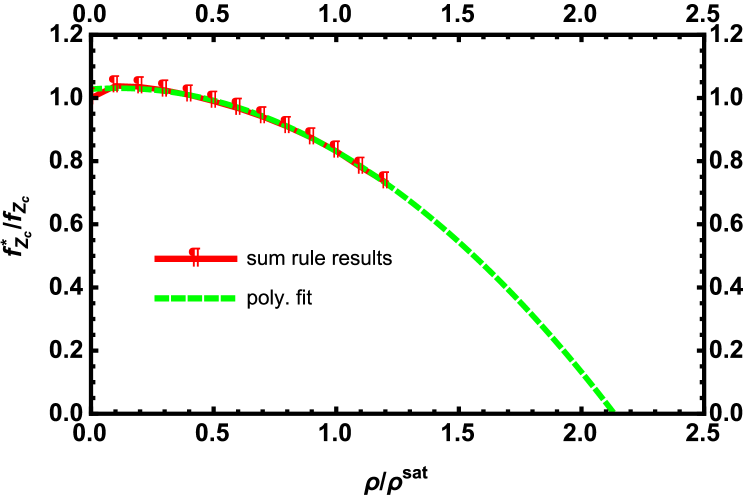
Figure 4: The ratios $m_{Z_{c}}^{*}/m_{Z_{c}}$ and $f_{Z_{c}}^{*}/f_{Z_{c}}$ as functions of $\rho/\rho^{sat}$ at mean values of the continuum threshold and Borel parameter.

It is necessary to check the results at higher densities using different fit functions that may end up in different predictions. Among various fit functions, the best ones are as follows: are obtained to be the above fit functions: exponential fit for the mass ratio and polynomial fit for the coupling constant ratio. Our analyses show that another set of fit functions, although not as good as the above selected functions, describe the behaviors of the quantities under study with respect to density, as well. These are the p-pole fit for $m_{Z_{c}}^{*}/m_{Z_{c}}$:

$$\frac{m_{Z_{c}}^{*}}{m_{Z_{c}}}=\frac{1}{\Big{[}1+\frac{x^{2}}{p~{}a}\Big{]}^{p}},$$ (22)

where $p=2.035$ and $a=3.056$, and exponential fit for $f_{Z_{c}}^{*}/f_{Z_{c}}$:

$$f_{Z_{c}}^{*}/f_{Z_{c}}=1.169-0.111e^{-x/0.879}.$$ (23)

In Figs. (5) and (6), we compare the predictions of these fit functions with the predictions of the previous fit functions. In the case of mass ratio, although both fitting results show a similar behavior, the p-pole fitting leads to a result, which is $6.4\%$ larger than the exponential fitting result at the density $5\rho^{sat}$. In the case of the coupling constant, $f_{Z_{c}}^{*}/f_{Z_{c}}$ becomes zero at $\rho/\rho^{sat}=2.13$ and $\rho/\rho^{sat}=2.07$, for the polynomial and exponential fittings, respectively. The small differences in the predictions of different fit functions remain inside the uncertainties allowed by the method used.

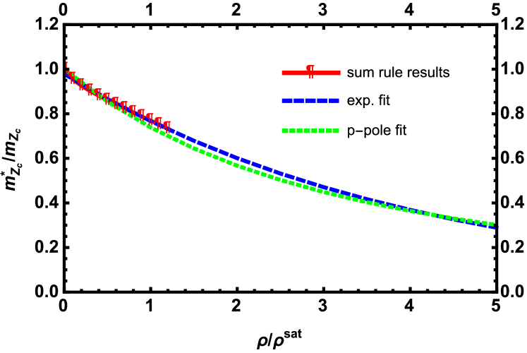
Figure 5: Comparison between exponential and p-pole fit functions for $m_{Z_{c}}^{*}/m_{Z_{c}}$ changes with respect to $\rho/\rho^{sat}$.

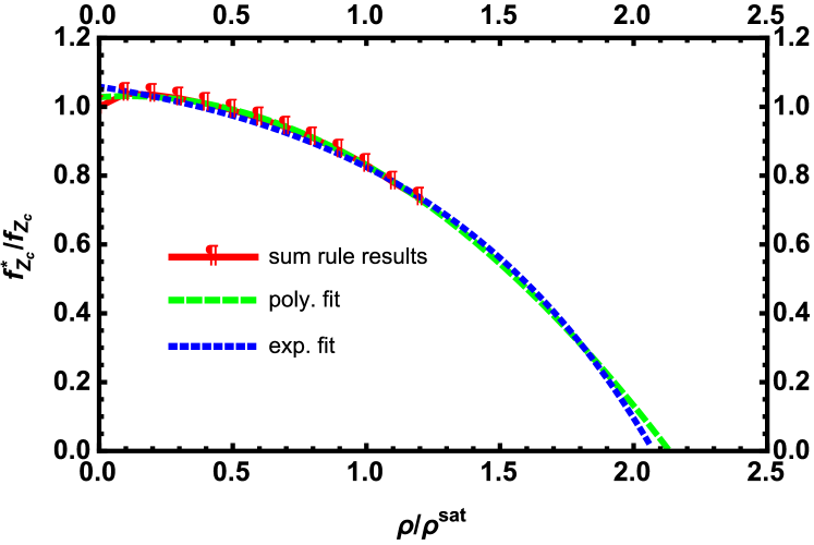
Figure 6: Comparison between polynomial and exponential fit functions for $f_{Z_{c}}^{*}/f_{Z_{c}}$ changes with respect to $\rho/\rho^{sat}$.

Now, we add the uncertainties in the values of the auxiliary parameters and errors of other inputs to the predictions at higher densities. For the case of best fits for the mass and coupling ratios, i.e., Eqs. (20) and (21) the swept areas presented in figure 7 are obtained. As it is seen, the values of the ratio $m_{Z_{c}}^{*}/m_{Z_{c}}$ vary in the region $[0.26,0.39]$ at $\rho/\rho^{sat}=5$. The band of coupling ratio $f_{Z_{c}}^{*}/f_{Z_{c}}$ becomes zero and crosses the $\rho/\rho^{sat}$ axis in the interval $[1.9,2.8]$.

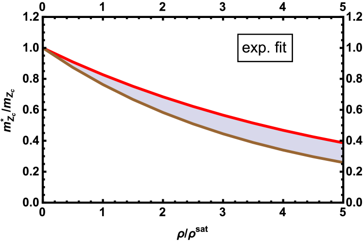
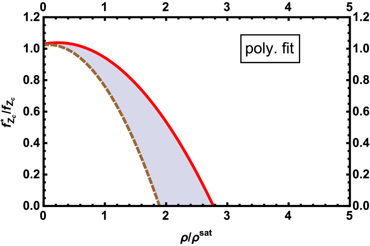
Figure 7: The ratios $m_{Z_{c}}^{*}/m_{Z_{c}}$ and $f_{Z_{c}}^{*}/f_{Z_{c}}$ as functions of $\rho/\rho^{sat}$ when the uncertainties of the auxiliary and other input parameters are considered.

IV Discussion and Conclusion

Despite a lot of experimental and theoretical effort, the structure, quark-gluon organization and nature of most exotic states remain unclear. The tetraquark state $Z_{c}(3900)$ is among the charmonium-like resonances that deserve more investigations in vacuum and a dense/hot medium in order to fix its nature. We considered it as a compact tetraquark and assigned a diquark-antidiquark structure to it with quantum numbers $J^{PC}=1^{+-}$. We constructed in-medium sum rules to calculate its mass, current-coupling and vector self-energy in the cold nuclear matter. The result obtained for its mass at $\rho\rightarrow 0$ limit is compatible with the experimental data and vacuum theory predictions. At saturation density, the mass and current coupling receive negative shifts with respect to the vacuum values. These shifts amount to $23\%$ and $15\%$ for the mass and current coupling, respectively. This state receives a repulsive vector self-energy with an amount of $32\%$ of its vacuum mass value at saturation nuclear matter density.

The in-medium experiments aim to reach higher densities. The neutron stars as the compact and dense objects are natural laboratories with densities $2-5$ times greater than the saturation nuclear matter density. The processes that occur at high densities may produce different kinds of hadrons, even the exotic states. Such experiments that take place in high densities will serve a good opportunity to study the exotic states like $Z_{c}$. Hence, to provide some phenomenological predictions, we investigated the behavior of the state under consideration with respect to density of the medium at higher densities. The in-medium sum rules are truncated at around $\rho/\rho^{sat}=(1-1.1)$. Thus, we used some fit functions in order to extrapolate the results to a density around $5\rho^{sat}$. Our analyses show that the mass and current coupling constant exhibit non-linear behavior and decrease with respect to density. The mass reaches to roughly $30\%$ of the vacuum mass at a density $5\rho^{sat}$ if the central values of auxiliary and other input parameters as well as the best fit are considered. When the uncertainties of the parameters are taken into account this value lies in the interval $[26\%,39\%]$. The current coupling however, rapidly decreases and goes to zero at a density $\approx 2.1\rho^{sat}$ if the central values of all parameters are considered, which may be considered as a pseudocritical density for melting of the exotic charmonium-like states. When the uncertainties in the values of the auxiliary and input parameters are taken into account, the band of $f_{Z_{c}}^{*}/f_{Z_{c}}$ becomes zero and crosses the $\rho/\rho^{sat}$ axis in the region $[1.9,2.8]$.

Investigation of properties of hadrons at finite temperature and density constitutes one of the main directions of the research in high energy and nuclear physics. Understanding the hadronic behavior under extreme conditions can help us not only understand the internal structure and nature of hadrons and gain knowledge of the QCD as the theory of the strong interaction, but also analyze the results of future experiments as well as understand different possible phases of matter.

V Appendix: Spectral Densities

We present the explicit forms of the spectral densities for the $g_{\mu\nu}$ structure used in the calculations:

$$\rho_{1}^{pert}(s) = -\frac{1}{3072\pi^{6}}\int_{0}^{1}dz\int_{0}^{1-z}dw\frac{1}{\xi\vartheta^{8}}\Bigg{[}wz\Big{[}(swz(w+z-1)-m_{c}^{2}\Big{[}(w^{3}+w^{2}(2z-1)$$ (24)

$$+ 2w(z-1)z+(z-1)z^{2}\Big{]}\Big{]}^{2}\Big{[}3m_{c}^{4}\Big{[}w^{3}+w^{2}(2z-1)+2w(z-1)z+(z-1)z^{2}\Big{]}^{2}$$

$$- 26m_{c}^{2}swz\Big{[}w^{4}+w^{3}(3z-2)+w^{2}(4z^{2}-5z+1)+wz(3z^{2}-5z+2)+(z-1)^{2}z^{2}\Big{]}$$

$$+ 35s^{2}w^{2}z^{2}(w+z-1)^{2}\Bigg{]}\Theta[L(s,z,w)],$$

$$\rho_{1}^{qq}(s) = \frac{1}{4\pi^{4}}\int_{0}^{1}dz\int_{0}^{1-z}dw\Bigg{\{}\frac{m_{c}w}{4\vartheta^{5}}\Bigg{[}3m_{c}^{4}\Big{[}w^{3}+w^{2}(2z-1)+2w(z-1)z+(z-1)z^{2}\Big{]}^{2}$$ (25)

$$- 10m_{c}^{2}swz\Big{[}w^{4}+w^{3}(3z-2)+w^{2}(4z^{2}-5z+1)+wz(3z^{2}-5z+2)+(z-1)^{2}z^{2}\Big{]}$$

$$+ 7s^{2}w^{2}z^{2}(w+z-1)^{2}\Bigg{]}\langle\bar{u}u\rangle_{\rho}+\frac{m_{q}m_{c}p_{0}w^{2}z\xi}{\vartheta^{5}}\Bigg{[}5m_{c}^{2}(w^{3}+w^{2}(2z-1)$$

$$+ 2w(z-1)z+(z-1)z^{2})-7swz\xi\Bigg{]}\langle u^{\dagger}u\rangle_{\rho}+\frac{m_{c}z}{4\vartheta^{5}}\Bigg{[}3m_{c}^{4}\Big{[}w^{3}+w^{2}(2z-1)$$

$$+ 2w(z-1)z+(z-1)z^{2}\Big{]}^{2}-10m_{c}^{2}swz\Big{[}w^{4}+w^{3}(3z-2)+w^{2}(4z^{2}-5z+1)$$

$$+ wz(3z^{2}-5z+2)+(z-1)^{2}z^{2}\Big{]}+7s^{2}w^{2}z^{2}(w+z-1)^{2}\Bigg{]}\langle\bar{d}d\rangle_{\rho}$$

$$+ \frac{m_{q}m_{c}p_{0}wz^{2}\xi}{\vartheta^{5}}\Bigg{[}5m_{c}^{2}(w^{3}+w^{2}(2z-1)+2w(z-1)z+(z-1)z^{2})-7swz\xi\Bigg{]}$$

$$\times \langle d^{\dagger}d\rangle_{\rho}\Bigg{\}}\Theta[L(s,z,w)],$$

$$\rho_{1}^{gg}(s) = \frac{1}{96\pi^{4}}\int_{0}^{1}dz\int_{0}^{1-z}dw\Bigg{\{}\Bigg{[}-i\frac{m_{q}m_{c}}{\vartheta^{4}}\Big{[}m_{c}^{2}\Big{(}4w^{6}z+w^{5}(24z^{2}-8z+1)$$ (26)

$$+ w^{4}(52z^{3}-44z^{2}+6z-1)+w^{3}z(60z^{3}-80z^{2}+55z-2)+w^{2}z^{2}(40z^{3}-68z^{2}$$

$$+ 95z-34)+6wz^{3}(2z^{3}-4z^{2}+13z-11)+33(z-1)z^{4}\Big{)}+wz\xi\Big{(}4p_{0}^{2}\big{(}4w^{3}z$$

$$+ w^{2}(16z^{2}-4z+1)+12w(z-1)z^{2}+z^{2}\big{)}-3s\Big{(}4w^{3}z+w^{2}(16z^{2}-4z+1)$$

$$+ 12w(z-1)z^{2}+17z^{2}\Big{)}\Big{)}\Big{]}\Bigg{]}\langle u^{\dagger}iD_{0}u\rangle_{\rho}+\frac{1}{1536(w-1)\xi^{2}\vartheta^{6}}\Bigg{[}m_{c}^{4}(w-1)\Big{(}w^{2}$$

$$+ w(z-1)+(z-1)z\Big{)}^{2}\Big{(}24w^{8}z+12w^{7}(11z^{2}-8z+3)+3w^{6}(112z^{3}-156z^{2}$$

$$+ 45z-36)+2w^{5}(258z^{4}-516z^{3}+332z^{2}-201z+54)+w^{4}(516z^{5}-1320z^{4}+1574z^{3}$$

$$- 1198z^{2}+471z-36)+w^{3}z(336z^{5}-1032z^{4}+1707z^{3}-1769z^{2}+858z-132)$$

$$+ w^{2}z^{2}(132z^{5}-468z^{4}+1122z^{3}-1253z^{2}+807z-180)+4wz^{3}(6z^{5}-24z^{4}+152z^{3}$$

$$- 155z^{2}+96z-27)+8z^{4}(23z^{3}-29z^{2}+9z-3)\Big{)}-m_{q}^{2}s(w-1)wz\Big{(}24w^{10}z$$

$$+ 12w^{9}(13z^{2}-12z+3)+w^{8}(492z^{3}-852z^{2}-89z-180)+w^{7}(984z^{4}-2424z^{3}+283z^{2}$$

$$+ 672z+360)+w^{6}(1368z^{5}-4296z^{4}+2149z^{3}+1121z^{2}-270z-360)+w^{5}(1368z^{6}$$

$$- -5160z^{5}+4057z^{4}-420z^{3}+275z^{2}-676z+180)+w^{4}(984z^{7}-4296z^{6}+4151z^{5}$$

$$- 809z^{4}+1804z^{3}-1901z^{2}+615z-36)+w^{3}z(492z^{7}-2424z^{6}+2485z^{5}+834z^{4}$$

$$+ 43z^{3}-2396z^{2}+1098z-132)+w^{2}z^{2}(156z^{7}-852z^{6}+898z^{5}$$

$$+ 1887z^{4}-2785z^{3}-27z^{2}+903z-180)+12w(z-1)^{2}z^{3}(2z^{5}-8z^{4}+18z^{3}+89z^{2}$$

$$- 12z-9)+8(z-1)^{3}z^{4}(23z^{2}+30z+3)\Big{)}-12swz^{2}(w+z-1)^{3}\Big{(}w^{5}((17s+4)z-4)$$

$$+ w^{4}(5(3s+2)z^{2}-2(17s+4)z+2)+w^{3}z(s(32z^{2}-13z+17)+4(3z^{2}-4z+1))$$

$$+ 2w^{2}z^{2}(s(16z^{2}-32z-1)+7z^{2}-10z+3)-8w(z-1)z^{3}(4s-z+1)+2w^{6}$$

$$+ 4(z-1)^{2}z^{4}\Big{)}\Bigg{]}\Big{\langle}\frac{\alpha_{s}}{\pi}G^{2}\Big{\rangle}_{\rho}\Bigg{\}}\Theta[L(s,z,w)],$$

and

$$\rho_{1}^{qgq}(s) = \int_{0}^{1}dz\int_{0}^{1-z}dw\Big{[}\rho_{1,1}^{qgq}(s)+\rho_{1,2}^{qgq}(s)+\rho_{1,3}^{qgq}(s)+\rho_{1,4}^{qgq}(s)+\rho_{1,5}^{qgq}(s)\Big{]}\Theta[L(s,z,w)],$$ (27)

where

$$\rho_{1,1}^{qgq}(s) = \frac{1}{96\pi^{4}}\Bigg{[}-\frac{m_{c}}{\kappa^{6}}\Big{[}m_{c}^{2}\Big{(}4w^{6}z+w^{5}(24z^{2}-8z+1)+w^{4}(52z^{3}-44z^{2}-2z-1)+w^{3}z$$ (28)

$$\times (60z^{3}-80z^{2}+31z+6)+w^{2}z^{2}(40z^{3}-68z^{2}+71z-18)+2wz^{3}(6z^{3}-12z^{2}$$

$$+ 35z-29)+33(z-1)z^{4}\Big{)}\Big{(}w^{2}+w(z-1)+(z-1)z\Big{)}^{3}+wz(w+z-1)\Big{(}4p_{0}^{2}(4w^{9}z$$

$$+ w^{8}(28z^{2}-16z+1)+3w^{7}(28z^{3}-36z^{2}+25z-1)+w^{6}(160z^{4}-300z^{3}+371z^{2}$$

$$- 169z+3)+w^{5}(208z^{5}-508z^{4}+838z^{3}-694z^{2}+157z-1)+w^{4}z(192z^{5}-564z^{4}$$

$$+ 1116z^{3}-1276z^{2}+567z-51)+2w^{3}z^{2}(62z^{5}-210z^{4}+463z^{3}-642z^{2}+409z-82)$$

$$+ w^{2}(z-1)^{2}z^{3}(52z^{3}-92z^{2}+239z-164)+3w(z-1)^{3}z^{4}(4z^{2}-4z+17)$$

$$+ (z-1)^{3}z^{5})-s\big{(}12w^{9}z+w^{8}(84z^{2}-48z+3)+w^{7}(252z^{3}-324z^{2}+121z-9)$$

$$+ w^{6}(480z^{4}-900z^{3}+713z^{2}-195z+9)+w^{5}(624z^{5}-1524z^{4}+1730z^{3}-986z^{2}$$

$$+ 159z-3)+w^{4}z(576z^{5}-1692z^{4}+2500z^{3}-2060z^{2}+709z-49)+2w^{3}z^{2}(186z^{5}$$

$$- 630z^{4}+1125z^{3}-1218z^{2}+635z-98)+w^{2}(z-1)^{2}z^{3}(156z^{3}-276z^{2}+589z-292)$$

$$+ w(z-1)^{3}z^{4}(36z^{2}-36z+193)+51(z-1)^{3}z^{5}\big{)}\Big{)}\Big{]}\Bigg{]}\langle\bar{u}iD_{0}iD_{0}u\rangle_{\rho},$$

$$\rho_{1,2}^{qgq}(s) = \frac{1}{12\pi^{4}}\Bigg{[}\frac{m_{c}wz^{2}\xi}{\vartheta^{7}}\Big{[}m_{c}^{2}(w+z)\Big{(}w^{2}+w(z-1)+(z-1)z\Big{)}^{3}-wz\xi$$ (29)

$$\times \Big{(}8p_{0}^{2}\big{(}3w^{4}+w^{3}(7z-6)+w^{2}(7z-6)+w^{2}(10z^{2}-14z+3)+wz(6z^{2}-13z+7)$$

$$+ 3(z-1)^{2}z^{2}\big{)}-s\big{(}5w^{4}+2w^{3}(6z-5)+w^{2}(17z^{2}-24z+5)+2wz(5z^{2}-11z$$

$$+ 6)+5(z-1)^{2}z^{2}\big{)}\Big{)}\Big{]}\Bigg{]}\langle\bar{d}iD_{0}iD_{0}d\rangle_{\rho},$$

$$\rho_{1,3}^{qgq}(s) = \frac{1}{96\pi^{4}}\Bigg{[}\frac{m_{c}}{4\vartheta^{7}}\Big{[}wz(w+z-1)\Big{(}2p_{0}^{2}(4w^{9}z+w^{8}(28z^{2}-16z+1)$$ (30)

$$+ 3w^{7}(28z^{3}-36z^{2}+25z-1)+w^{6}(160z^{4}-300z^{3}+371z^{2}$$

$$- 169m_{c}z+3)+w^{5}(208z^{5}-508z^{4}+838z^{3}-694z^{2}+157z-1)+w^{4}z$$

$$\times (192z^{5}-564z^{4}+1116z^{3}-1276z^{2}+567z-51)+2w^{3}z^{2}(62z^{5}-210z^{4}$$

$$+ 463z^{3}-642z^{2}+409z-82)+w^{2}(z-1)^{2}z^{3}(52z^{3}-92z^{2}+239z$$

$$- 164)+3w(z-1)^{3}z^{4}(4z^{2}-4z+17)+(z-1)^{3}z^{5})+s(4w^{9}z+w^{8}(28z^{2}$$

$$- 16z-59)+w^{7}(84z^{3}-108z^{2}-401z+177)+w^{6}(160z^{4}-300z^{3}-1197z^{2}$$

$$+ 1259z-177)+w^{5}(208z^{5}-508z^{4}-2022z^{3}+3534z^{2}-1271z+59)$$

$$+ w^{4}z(192z^{5}-564z^{4}-2204z^{3}+5368z^{2}-3185z+425)+2w^{3}z^{2}(62z^{5}-210z^{4}$$

$$- 751z^{3}+2380z^{2}-1945z+464)+w^{2}(z-1)^{2}z^{3}(52z^{3}-92z^{2}-861z+760)$$

$$+ w(z-1)^{3}z^{4}(12z^{2}-12z-173)+25(z-1)^{3}z^{5})\Big{)}-m_{c}^{2}(w^{2}+w(z-1)$$

$$+ (z-1)z)^{3}\Big{(}4w^{6}z+w^{5}(24z^{2}-8z-35)+w^{4}(52z^{3}-44z^{2}-170z+35)+w^{3}z(60z^{3}$$

$$- 80z^{2}-353z+174)+w^{2}z^{2}(40z^{3}-68z^{2}-301z+234)+2wz^{3}(6z^{3}-12z^{2}-37z$$

$$+ 43)+9(z-1)z^{4}\Big{)}\Big{]}\Bigg{]}\langle\bar{u}g_{s}\sigma Gu\rangle_{\rho},$$

$$\rho_{1,4}^{qgq}(s) = \frac{1}{48\pi^{4}}\Bigg{[}\frac{m_{c}wz^{2}\xi}{\vartheta^{7}}\Big{[}13m_{c}^{2}(w+z)\Big{(}w^{2}+w(z-1)+(z-1)z\Big{)}^{3}+wz\xi$$ (31)

$$\times \Big{(}4p_{0}^{2}\big{(}3w^{4}+w^{3}(7z-6)+w^{2}(10z^{2}-14z+3)+wz(6z^{2}-13z+7)$$

$$+ 3(z-1)^{2}z^{2}\big{)}-s\big{(}31w^{4}+w^{3}(66z-62)+w^{2}(97z^{2}-132z+31)+2wz(31z^{2}-64z$$

$$+ 33)+31(z-1)^{2}z^{2}\big{)}\Big{)}\Big{]}\Bigg{]}\langle\bar{d}g_{s}\sigma Gd\rangle_{\rho},$$

and

$$\rho_{1,5}^{qgq}(s) = \frac{1}{192\pi^{4}}\Bigg{[}\frac{p_{0}z}{\vartheta^{4}}\Big{[}m_{c}^{2}\Big{(}16w^{7}z+w^{6}(48z^{2}-48z+31)+w^{5}(80z^{3}-128z^{2}+137z-62)$$ (32)

$$+ w^{4}(80z^{4}-176z^{3}+237z^{2}-164z+31)+w^{3}z(48z+4-128z^{3}+223z^{2}-190z+59)$$

$$+ w^{2}z^{2}(16z^{4}-48z^{3}+109z^{2}-110z+33)+wz^{3}(25z^{2}-38z+13)$$

$$+ 8(z-1)^{2}z^{4}\big{)}\Big{]}\Bigg{]}\langle u^{{\dagger}}g_{s}\sigma Gu\rangle_{\rho}.$$

The shorthand notations in the above equations are given as

$$\xi = (w+z-1),$$

$$\vartheta = (w^{2}+w(z-1)+(z-1)z),$$

$$L[s,w,z] = \frac{((-1+w)(-(swz(-1+w+z))+m_{c}^{2}(w^{3}+2w(-1+z)z+(-1+z)z^{2}+w^{2}(-1+2z))))}{(w^{2}+w(-1+z)+(-1+z)z)^{2}}.$$ (33)

References

-
(1)
M. Tanabashi, et al.,
Review of particle
physics, Phys. Rev. D 98 (2018) 030001.
URL https://link.aps.org/doi/10.1103/PhysRevD.98.030001 -
(2)
Y.-R. Liu, H.-X. Chen, W. Chen, X. Liu, S.-L. Zhu,
Pentaquark
and tetraquark states, Progress in Particle and Nuclear Physics 107 (2019)
237 – 320.
URL http://www.sciencedirect.com/science/article/pii/S0146641019300304 -
(3)
F.-K. Guo, C. Hanhart, U.-G. Meißner, Q. Wang, Q. Zhao, B.-S. Zou,
Hadronic
molecules, Rev. Mod. Phys. 90 (2018) 015004.
URL https://link.aps.org/doi/10.1103/RevModPhys.90.015004 -
(4)
A. Ali, J. S. Lange, S. Stone,
Exotics:
Heavy pentaquarks and tetraquarks, Progress in Particle and Nuclear Physics
97 (2017) 123 – 198.
URL http://www.sciencedirect.com/science/article/pii/S0146641017300716 -
(5)
S. L. Olsen, T. Skwarnicki, D. Zieminska,
Nonstandard
heavy mesons and baryons: Experimental evidence, Rev. Mod. Phys. 90 (2018)
015003.
URL https://link.aps.org/doi/10.1103/RevModPhys.90.015003 -
(6)
P. C. Wallbott, G. Eichmann, C. S. Fischer,
as a
four-quark state in a Dyson-Schwinger/Bethe-Salpeter approach, Phys. Rev.
D 100 (2019) 014033.
URL https://link.aps.org/doi/10.1103/PhysRevD.100.014033 -
(7)
S.-Q. Luo, K. Chen, X. Liu, Y.-R. Liu, S.-L. Zhu,
Exotic tetraquark
states with the configuration, The European Physical
Journal C 77 (10) (2017) 709.
URL https://doi.org/10.1140/epjc/s10052-017-5297-4 -
(8)
V. Baru, C. Hanhart, A. V. Nefediev,
Can be the tensor
partner of the ?, Journal of High Energy Physics 2017 (6) (2017)
10.
URL https://doi.org/10.1007/JHEP06(2017)010 -
(9)
F. E. Close, P. R. Page,
The
threshold resonance, Physics Letters B 578 (1) (2004)
119 – 123.
URL http://www.sciencedirect.com/science/article/pii/S0370269303015843 -
(10)
E. Braaten, M. Lu,
Line shapes of the
, Phys. Rev. D 76 (2007) 094028.
URL https://link.aps.org/doi/10.1103/PhysRevD.76.094028 -
(11)
S. Coito, G. Rupp, E. van Beveren,
is not a
true molecule, The European Physical Journal C 73 (3) (2013) 2351.
URL https://doi.org/10.1140/epjc/s10052-013-2351-8 -
(12)
X. Liu, Y.-R. Liu, W.-Z. Deng, S.-L. Zhu,
Is
a loosely bound molecular state?, Phys. Rev. D 77 (2008) 034003.
URL https://link.aps.org/doi/10.1103/PhysRevD.77.034003 -
(13)
C.-Y. Cui, X.-H. Liao, Y.-L. Liu, M.-Q. Huang,
Could
be a molecular
state?, Journal of Physics G: Nuclear and Particle Physics 41 (7) (2014)
075003.
URL https://doi.org/10.1088%2F0954-3899%2F41%2F7%2F075003 -
(14)
Q. Wang, C. Hanhart, Q. Zhao,
Decoding the
riddle of and , Phys. Rev. Lett. 111 (2013)
132003.
URL https://link.aps.org/doi/10.1103/PhysRevLett.111.132003 -
(15)
A. Esposito, A. Pilloni, A. Polosa,
Hybridized
tetraquarks, Physics Letters B 758 (2016) 292 – 295.
URL http://www.sciencedirect.com/science/article/pii/S0370269316301757 -
(16)
N. Isgur, R. Kokoski, J. Paton,
Gluonic
excitations of mesons: Why they are missing and where to find them, Phys.
Rev. Lett. 54 (1985) 869–872.
URL https://link.aps.org/doi/10.1103/PhysRevLett.54.869 -
(17)
For the Hadron Spectrum collaboration, L. Liu, G. Moir, M. Peardon, S. M.
Ryan, C. E. Thomas, P. Vilaseca, J. J. Dudek, R. G. Edwards, B. Joó,
D. G. Richards, Excited and
exotic charmonium spectroscopy from lattice QCD, Journal of High Energy
Physics 2012 (7) (2012) 126.
URL https://doi.org/10.1007/JHEP07(2012)126 -
(18)
G. Li, Hidden-charmonium
decays of and in intermediate meson loops model,
The European Physical Journal C 73 (11) (2013) 2621.
URL https://doi.org/10.1140/epjc/s10052-013-2621-5 -
(19)
J.-R. Zhang,
Improved QCD sum
rule study of as a molecular state,
Phys. Rev. D 87 (2013) 116004.
URL https://link.aps.org/doi/10.1103/PhysRevD.87.116004 -
(20)
S. H. Blitz, R. F. Lebed,
Tetraquark cusp
effects from diquark pair production, Phys. Rev. D 91 (2015) 094025.
URL https://link.aps.org/doi/10.1103/PhysRevD.91.094025 -
(21)
E. S. Swanson, Cusps and
exotic charmonia, Int. J. Mod. Phys. E25 (2016) 1642010.
URL https://doi.org/10.1142/S0218301316420106 -
(22)
P. Pakhlov, T. Uglov,
Charged
charmonium-like from rescattering in conventional
decays, Physics Letters B 748 (2015) 183 – 186.
URL http://www.sciencedirect.com/science/article/pii/S0370269315005043 -
(23)
F.-K. Guo, C. Hanhart, Q. Wang, Q. Zhao,
Could the
near-threshold states be simply kinematic effects?, Phys. Rev. D 91
(2015) 051504.
URL https://link.aps.org/doi/10.1103/PhysRevD.91.051504 -
(24)
S. Dubynskiy, M. Voloshin,
Hadro-charmonium,
Physics Letters B 666 (4) (2008) 344 – 346.
URL http://www.sciencedirect.com/science/article/pii/S0370269308009465 -
(25)
X. Li, M. B. Voloshin,
(4260) and (4360) as
mixed hadrocharmonium, Mod. Phys. Lett. A29 (12) (2014) 1450060.
URL https://doi.org/10.1142/S0217732314500606 -
(26)
M. Ablikim, et al.,
Observation of
a charged charmoniumlike structure in
at , Phys. Rev. Lett.
110 (2013) 252001.
URL https://link.aps.org/doi/10.1103/PhysRevLett.110.252001 -
(27)
Z. Q. Liu, et al.,
Study of
and observation of a charged charmoniumlike state at Belle, Phys. Rev.
Lett. 110 (2013) 252002.
URL https://link.aps.org/doi/10.1103/PhysRevLett.110.252002 -
(28)
B. Aubert, et al.,
Observation of
a broad structure in the
mass spectrum around , Phys. Rev.
Lett. 95 (2005) 142001.
URL https://link.aps.org/doi/10.1103/PhysRevLett.95.142001 -
(29)
Q. He, et al.,
Confirmation of
the resonance production in initial state radiation, Phys. Rev.
D 74 (2006) 091104.
URL https://link.aps.org/doi/10.1103/PhysRevD.74.091104 -
(30)
C. Z. Yuan, et al.,
Measurement of
the
cross section via initial-state radiation at belle, Phys. Rev. Lett. 99
(2007) 182004.
URL https://link.aps.org/doi/10.1103/PhysRevLett.99.182004 -
(31)
T. Xiao, S. Dobbs, A. Tomaradze, K. K. Seth,
Observation
of the charged hadron and evidence for the neutral
in at
MeV, Physics Letters B 727 (4) (2013) 366 – 370.
URL http://www.sciencedirect.com/science/article/pii/S0370269313008484 -
(32)
M. Ablikim, et al.,
Observation of
a charged mass peak
in
at , Phys. Rev. Lett. 112 (2014)
022001.
URL https://link.aps.org/doi/10.1103/PhysRevLett.112.022001 -
(33)
M. Ablikim, et al.,
Observation of
in
,
Phys. Rev. Lett. 115 (2015) 112003.
URL https://link.aps.org/doi/10.1103/PhysRevLett.115.112003 -
(34)
M. Ablikim, et al.,
Confirmation of a
charged charmoniumlike state in
with double tag, Phys. Rev. D 92 (2015) 092006.
URL https://link.aps.org/doi/10.1103/PhysRevD.92.092006 -
(35)
M. Ablikim, et al.,
Observation of
a neutral structure near the mass threshold in
at and 4.257 gev, Phys. Rev. Lett. 115 (2015) 222002.
URL https://link.aps.org/doi/10.1103/PhysRevLett.115.222002 -
(36)
V. M. Abazov, et al.,
Evidence for
in semi-inclusive decays of
-flavored hadrons, Phys. Rev. D 98 (2018) 052010.
URL https://link.aps.org/doi/10.1103/PhysRevD.98.052010 - (37) C. Liu, L. Liu, K.-L. Zhang, Towards the understanding of from lattice QCDarXiv:1911.08560.
-
(38)
L. S. Kisslinger, S. Casper,
Zc(3900) as a four-quark
state, International Journal of Theoretical Physics 54 (10) (2015)
3825–3830.
doi:10.1007/s10773-015-2623-1.
URL https://doi.org/10.1007/s10773-015-2623-1 -
(39)
S. S. Agaev, K. Azizi, H. Sundu,
Strong
;
decays in qcd, Phys. Rev. D
93 (2016) 074002.
URL https://link.aps.org/doi/10.1103/PhysRevD.93.074002 -
(40)
S. S. Agaev, K. Azizi, H. Sundu,
Treating
and as the ground state and first radially excited
tetraquarks, Phys. Rev. D 96 (2017) 034026.
URL https://link.aps.org/doi/10.1103/PhysRevD.96.034026 -
(41)
W. Chen, T. G. Steele, H.-X. Chen, S.-L. Zhu,
Mass spectra of
and exotic states as hadron molecules, Phys. Rev. D 92
(2015) 054002.
URL https://link.aps.org/doi/10.1103/PhysRevD.92.054002 -
(42)
Y. Dong, A. Faessler, T. Gutsche, V. E. Lyubovitskij,
Strong decays of
molecular states and
, Phys. Rev. D 88 (2013) 014030.
URL https://link.aps.org/doi/10.1103/PhysRevD.88.014030 -
(43)
S. Patel, M. Shah, P. C. Vinodkumar,
Mass spectra of four-quark
states in the hidden charm sector, The European Physical Journal A 50 (8)
(2014) 131.
URL https://doi.org/10.1140/epja/i2014-14131-9 -
(44)
K. Azizi, N. Er,
X(3872):
propagating in a dense medium, Nuclear Physics B 936 (2018) 151 – 168.
URL http://www.sciencedirect.com/science/article/pii/S055032131830261X -
(45)
T. Cohen, R. Furnstahl, D. Griegel, X. Jin,
QCD
sum rules and applications to nuclear physics, Progress in Particle and
Nuclear Physics 35 (1995) 221 – 298.
URL http://www.sciencedirect.com/science/article/pii/014664109500043I -
(46)
R. J. Furnstahl, D. K. Griegel, T. D. Cohen,
QCD sum rules for
nucleons in nuclear matter, Phys. Rev. C 46 (1992) 1507–1527.
URL https://link.aps.org/doi/10.1103/PhysRevC.46.1507 -
(47)
B. Ioffe,
QCD
(Quantum chromodynamics) at low energies, Progress in Particle and Nuclear
Physics 56 (1) (2006) 232 – 277.
URL http://www.sciencedirect.com/science/article/pii/S0146641005000736 -
(48)
X. Jin, T. D. Cohen, R. J. Furnstahl, D. K. Griegel,
QCD sum rules for
nucleons in nuclear matter ii, Phys. Rev. C 47 (1993) 2882–2900.
URL https://link.aps.org/doi/10.1103/PhysRevC.47.2882 -
(49)
P. E. Shanahan, A. W. Thomas, R. D. Young,
Sigma terms from
an SU(3) chiral extrapolation, Phys. Rev. D 87 (2013) 074503.
URL https://link.aps.org/doi/10.1103/PhysRevD.87.074503 -
(50)
N. Er, K. Azizi,
Fate of the doubly
heavy spin- baryons in a dense medium, Phys. Rev. D 99 (2019) 074012.
URL https://link.aps.org/doi/10.1103/PhysRevD.99.074012 -
(51)
K. Azizi, N. Er,
Effects of a
dense medium on parameters of doubly heavy baryons, Phys. Rev. D 100 (2019)
074004.
URL https://link.aps.org/doi/10.1103/PhysRevD.100.074004 -
(52)
A. Pilloni, C. Fernández-Ramírez, A. Jackura, V. Mathieu, M. Mikhasenko,
J. Nys, A. Szczepaniak,
Amplitude
analysis and the nature of the , Physics Letters B 772 (2017)
200 – 209.
URL http://www.sciencedirect.com/science/article/pii/S0370269317305063 -
(53)
Z.-G. Wang, T. Huang,
Analysis of the
, , and as axial-vector tetraquark
states with qcd sum rules, Phys. Rev. D 89 (2014) 054019.
URL https://link.aps.org/doi/10.1103/PhysRevD.89.054019 -
(54)
Z.-G. Wang, T. Huang,
Possible assignments of
the , , and as axial-vector molecular
states, The European Physical Journal C 74 (5) (2014) 2891.
URL https://doi.org/10.1140/epjc/s10052-014-2891-6 -
(55)
K. Kim, H. K. Lee, J. Lee,
Compact Star Matter: EoS
with New Scaling Law, Int. J. Mod. Phys. E26 (2017) 1740011.
URL https://doi.org/10.1142/S0218301317400110