The Asymptotic Distribution of the MLE in High-Dimensional Logistic Models: Arbitrary Covariance

Abstract

We study the distribution of the maximum likelihood estimate (MLE) in high-dimensional logistic models, where covariates are Gaussian with an arbitrary covariance structure. We prove that in the limit of large problems holding the ratio between the number $p$ of covariates and the sample size $n$ constant, every finite list of MLE coordinates follows a multivariate normal distribution. Concretely, the $j$th coordinate $\hat{\beta}_{j}$ of the MLE is asymptotically normally distributed with mean $\alpha_{\star}\beta_{j}$ and standard deviation $\sigma_{\star}/\tau_{j}$; here, $\beta_{j}$ is the value of the true regression coefficient, and $\tau_{j}$ the standard deviation of the $j$th predictor conditional on all the others. The numerical parameters $\alpha_{\star}>1$ and $\sigma_{\star}$ only depend upon the problem dimensionality $p/n$ and the overall signal strength, and can be accurately estimated. Our results imply that the MLE’s magnitude is biased upwards and that the MLE’s standard deviation is greater than that predicted by classical theory. We present a series of experiments on simulated and real data showing excellent agreement with the theory.

, and

1 Introduction

Logistic regression is the most widely applied statistical model for fitting a binary response from a list of covariates. This model is used in a great number of disciplines ranging from social science to biomedical studies. For instance, logistic regression is routinely used to understand the association between the susceptibility of a disease and genetic and/or environmental risk factors.

A logistic model is usually constructed by the method of maximum likelihood (ML) and it is therefore critically important to understand the properties of ML estimators (MLE) in order to test hypotheses, make predictions and understand their validity. In this regard, assuming the logistic model holds, classical ML theory provides the asymptotic distribution of the MLE when the number of observations $n$ tends to infinity while the number $p$ of variables remains constant. In a nutshell, the MLE is asymptotically normal with mean equal to the true vector of regression coefficients and variance equal to $\mathcal{I}^{-1}_{\boldsymbol{\beta}}$, where $\mathcal{I}_{\boldsymbol{\beta}}$ is the Fisher information evaluated at true coefficients [26, Appendix A], [42, Chapter 5]. Another staple of classical ML theory is that the extensively used likelihood ratio test (LRT) asymptotically follows a chi-square distribution under the null, a result known as Wilk’s theorem [44][42, Chapter 16]. Again, this holds in the limit where $p$ is fixed and $n\rightarrow\infty$ so that the dimensionality $p/n$ is vanishingly small. (See [28, 29, 30, 19, 16, 1] for the relevance of these classical results under diverging dimensions with $p$ negligible compared to $n$.)

1.1 High-dimensional maximum-likelihood theory

Against this background, a recent paper [38] showed that the classical theory does not even approximately hold in large sample sizes if $p$ is not negligible compared to $n$. In more details, empirical and theoretical analyses in [38] establish the following conclusions:

1. The MLE is biased in that it overestimates the true effect magnitudes.

2. The variance of the MLE is larger than that implied by the inverse Fisher information.

3. The LRT is not distributed as a chi-square variable; it is stochastically larger than a chi-square.

Under a suitable model for the covariates, [38] developed formulas to calculate the asymptotic bias and variance of the MLE under a limit of large samples where the ratio $p/n$ between the number of variables and the sample size has a positive limit $\kappa$. Operationally, these results provide an excellent approximation of the distribution of the MLE in large logistic models in which the number of variables obey $p\approx\kappa\,n$ (this is the same regime as that considered in random matrix theory when researchers study the eigenvalue distribution of sample covariance matrices in high dimensions). Furthermore, [38] also proved that the LRT is asymptotically distributed as a fixed multiple of a chi-square, with a multiplicative factor that can be determined.

1.2 This paper

The asymptotic distribution of the MLE in high-dimensional logistic regression briefly reviewed above holds for models in which the covariates are independent and Gaussian. This is the starting point of this paper: since features typically encountered in applications are not independent, it is important to describe the behavior of the MLE under models with arbitrary covariance structures. In this work, we shall limit ourselves to Gaussian covariates although we believe our results extend to a wide class of distributions with sufficiently light tails (we provide numerical evidence supporting this claim).

To give a glimpse of our results, imagine we have $n$ independent pairs of observations $(\boldsymbol{x}_{i},y_{i})$, where the features $\boldsymbol{x}_{i}\in\mathbb{R}^{p}$ and the class label $y_{i}\in\{-1,1\}$. We assume that the $\boldsymbol{x}_{i}$’s follow a multivariate normal distribution with mean zero and arbitrary covariance, and that the likelihood of the class label $y_{i}$ is related to $\boldsymbol{x}_{i}$ through the logistic model

$$\operatorname{\mathbb{P}}(y_{i}=1\>|\>\boldsymbol{x}_{i})=1/(1+e^{-\boldsymbol{x}_{i}^{\top}\boldsymbol{\beta}}).$$ (1.1)

Denote the MLE for estimating the parameters $\boldsymbol{\beta}$ by $\hat{\boldsymbol{\beta}}$ and consider centering and scaling $\hat{\boldsymbol{\beta}}$ via

$$T_{j}=\frac{\sqrt{n}(\hat{\beta}_{j}-\alpha_{\star}\beta_{j})}{\sigma_{\star}/\tau_{j}};$$ (1.2)

here, $\tau_{j}$ is the standard deviation of the $j$th feature variable (the $j$th component of $\boldsymbol{x}_{i}$) conditional on all the other variables (all the other components of $\boldsymbol{x}_{i}$), whereas $\alpha_{\star}>1$ and $\sigma_{\star}$ are numerical parameters we shall determine in Section 3.2. Then after establishing a stochastic representation for the MLE which is valid for every finite $n$ and $p$, this paper proves two distinct asymptotic results (both hold in the same regime where $n$ and $p$ diverge to infinity in a fixed ratio).

The first concerns marginals of the MLE. Under some conditions on the magnitude of the regression coefficient $\beta_{j}$, we show that

$$T_{j}\,\,\stackrel{{\scriptstyle\mathrm{d}}}{{\longrightarrow}}\,\,\mathcal{N}(0,1),$$ (1.3)

and demonstrate an analogous statement for the distribution of any finite collection of coordinates. The meaning is clear; if the statistician is given several data sets from the model above and computes a given regression coefficient for each via ML, then the histogram of these coefficients across all data sets will look approximately Gaussian.

This state of affairs extends [38, Theorem 3] significantly, which established the joint distribution of a finite collection of null coordinates, in the setting of independent covariates. Specifically,

1. Eqn. (1.3) is true when covariates have arbitrary covariance structure.

2. Eqn. (1.3) holds for both null and non-null coordinates.

The second asymptotic result concerns the empirical distribution of the MLE in a single data set/realization: we prove that the empirical distribution of the $T_{j}$’s converges to a standard normal in the sense that,

$$\frac{\#\{j:T_{j}\leq t\}}{p}\stackrel{{\scriptstyle\mathrm{P}}}{{\longrightarrow}}\,\,\mathbb{P}(\mathcal{N}(0,1)\leq t).$$ (1.4)

This means that if we were to plot the histogram of all the $T_{j}$’s obtained from a single data set, we would just see a bell curve. Another consequence is that for sufficiently nice functions $f(\cdot)$, we have

$$\frac{1}{p}\sum_{j=1}^{p}f(T_{j})\,\,\stackrel{{\scriptstyle\textrm{P}}}{{\longrightarrow}}\,\,\mathbb{E}\left[f(Z)\right],$$ (1.5)

where $Z\sim\mathcal{N}(0,1)$. For instance, taking $f$ to be the absolute value—we use the caveat that $f$ is not uniformly bounded—we would conclude that

$$\frac{1}{p}\sum_{j=1}^{p}\sqrt{n}\,\tau_{j}|\hat{\beta}_{j}-\alpha_{\star}\beta_{j}|\,\,\stackrel{{\scriptstyle\textrm{P}}}{{\longrightarrow}}\,\,\sigma_{\star}\,\sqrt{2/{\pi}}.$$

Taking $f$ to be the indicator function of the interval $[-1.96,1.96]$, we would see that

$$\frac{1}{p}\sum_{j=1}^{p}1\left\{-1.96\leq\frac{\sqrt{n}(\hat{\beta}_{j}-\alpha_{\star}\beta_{j})}{\sigma_{\star}/\tau_{j}}\leq 1.96\right\}\,\,\stackrel{{\scriptstyle\textrm{P}}}{{\longrightarrow}}\,\,0.95.$$

Hence, the miscoverage rate (averaged over all variables) of the confidence intervals

$$[\hat{\beta}_{j}^{-},\hat{\beta}_{j}^{+}],\qquad\hat{\beta}_{j}^{\pm}=\frac{\hat{\beta}_{j}\pm 1.96\sigma_{\star}/\sqrt{n}\tau_{j}}{\alpha_{\star}},$$

in a single experiment would approximately be equal to 5%.

Finally, this paper extends the LRT asymptotics to the case of arbitrary covariance.

We provide an R package “glmhd” available on GitHub [47], which provides functionality to compute the parameters $\alpha_{\star}$, $\sigma_{\star}$ discussed above and $\lambda_{\star}$ introduced below, as well as functionality to analyze real datasets.

1.3 Technical contributions

We derive the asymptotic distribution of every finite collection of MLE coordinates (Theorem 3.1). In [38], the authors studied the distribution of the MLE corresponding to a null variable, building upon leave-one-out techniques [14, 15], alternatively known as the cavity method in statistical physics [25]. The crucial issue here is that it is not clear how to apply leave-one-out techniques when analyzing non-null coordinates. Consequently, the novelty lies in recognizing that studying the MLE when covariates are correlated Gaussian is equivalent to studying the MLE when covariates are i.i.d. Gaussian and there is only a single non-null. This connection is crucial for Theorem 3.1, which relies on the new [46, Proposition B.1] and Lemma 2.1. Theorem 3.1 also gives the distribution of linear combinations for arbitrarily correlated Gaussian covariates—a setting beyond the reach of the techniques from [38].

The technique to establish the limiting empirical distribution of the MLE is a distinct contribution. We show that for every $n$ and $p$, the MLE can be represented as a function of a correlated Gaussian vector that has empirical distribution converging to a standard normal. This representation [46, Proposition B.1] presented in the supplementary material is new. Prior work [38] proved a version of (1.4) utilizing the framework of generalized approximate message passing [32, 20, 7] (G-AMP). These proofs relied on the assumption of i.i.d. entries on the design matrix. For correlated matrices, other ideas are needed.

In a broader context, hypothesis testing and confidence interval construction for high-dimensional regression models have been extensively studied in the past decade, and even earlier [4, 43]. Here, we mention the threads of research in the high-dimensional regime (3.1) that are most relevant for this paper, deferring a detailed survey to [24, 39]. In [14, 15, 6, 41, 5, 10], the authors studied high-dimensional estimation and inference for linear models using seemingly disparate technical ingredients—leave-one-out [14, 15, 25], approximate message passing (AMP)[13, 8], the Convex Gaussian Min-Max Theorem (CGMT) [18, stojnic2013framework, 40, 41], second-order Poincare inequalities [11] and debiasing [17, 45, 21]. (See [22, 12, 27] for some other works around debiasing that consider a different high-dimensional regime.) Utilizing similar techniques, [38, 37, 7, 34] studied high-dimensional inference for generalized linear models with i.i.d. Gaussian designs.

2 A stochastic representation of the MLE

We consider a setting with $n$ independent observations $(\boldsymbol{x}_{i},y_{i})_{i=1}^{n}$ such that the covariates $\boldsymbol{x}_{i}\in\mathbb{R}^{p}$ follow a multivariate normal distribution $\boldsymbol{x}_{i}\sim\mathcal{N}(\boldsymbol{0},\boldsymbol{\Sigma})$, with covariance $\boldsymbol{\Sigma}\in\mathbb{R}^{p\times p}$, and the response $y_{i}\in\{-1,1\}$ follows the logistic model (1.1) with regression coefficients $\boldsymbol{\beta}\in\mathbb{R}^{p}$. We assume that $\boldsymbol{\Sigma}$ has full column rank so that the model is identifiable. The maximum likelihood estimator (MLE) $\hat{\boldsymbol{\beta}}$ optimizes the log-likelihood function

$$\ell(\boldsymbol{b};\boldsymbol{X},\boldsymbol{y})=\sum_{i=1}^{n}-\log(1+\exp(-y_{i}\boldsymbol{x}_{i}^{\top}\boldsymbol{b}))$$ (2.1)

over all $\boldsymbol{b}\in\mathbb{R}^{p}$. (Here and below, $\boldsymbol{X}$ is the $n\times p$ matrix of covariates and $\boldsymbol{y}$ the $n\times 1$ vector of responses.)

2.1 From dependent to independent covariates

We begin our discussion by arguing that the aforementioned setting of dependent covariates can be translated to that of independent covariates. This follows from the invariance of the Gaussian distribution with respect to linear transformations.

Proposition 2.1.

Fix any matrix $\boldsymbol{L}$ obeying $\boldsymbol{\Sigma}=\boldsymbol{L}\boldsymbol{L}^{\top}$, and consider the vectors

$$\hat{\boldsymbol{\theta}}:=\boldsymbol{L}^{\top}\hat{\boldsymbol{\beta}}\qquad\mathrm{and}\qquad\boldsymbol{\theta}:=\boldsymbol{L}^{\top}\boldsymbol{\beta}.$$ (2.2)

Then $\hat{\boldsymbol{\theta}}$ is the MLE in a logistic model with regression coefficient $\boldsymbol{\theta}$ and covariates drawn i.i.d. from $\mathcal{N}(\boldsymbol{0},\boldsymbol{I}_{p})$.

Proof.

Because the likelihood (2.1) depends on the $\boldsymbol{x}_{i}$’s and $\boldsymbol{b}$ only through their inner product,

$$\ell(\boldsymbol{b};\boldsymbol{X},\boldsymbol{y})=\ell(\boldsymbol{L}^{\top}\boldsymbol{b};\boldsymbol{X}\boldsymbol{L}^{-\top},\boldsymbol{y})$$ (2.3)

for every $\boldsymbol{b}\in\mathbb{R}^{p}$. If $\hat{\boldsymbol{\beta}}$ is the MLE of the original model, then $\hat{\boldsymbol{\theta}}=\boldsymbol{L}^{\top}\hat{\boldsymbol{\beta}}$ is the MLE of a logistic model whose covariates are i.i.d. draws from $\mathcal{N}(\boldsymbol{0},\boldsymbol{I}_{p})$, and true regression coefficients given by $\boldsymbol{\theta}=\boldsymbol{L}^{\top}\boldsymbol{\beta}$. ∎

Proposition 2.1 has a major consequence—for an arbitrary variable $j$, which we can assume to be the last variable by permuting the order of the variables, we may choose $\boldsymbol{\Sigma}=\boldsymbol{L}\boldsymbol{L}^{\top}$ to be a Cholesky factorization of the covariance matrix, such that $\boldsymbol{x}_{i}$ can be expressed as

$$\underbrace{\begin{bmatrix}\star\\ \star\\ \star\\ x_{i,j}\end{bmatrix}}_{\boldsymbol{x}_{i}}=\underbrace{\begin{bmatrix}\star&&&\\ \star&\star&&\\ \star&\star&\star&\\ \star&\star&\star&\tau_{j}\end{bmatrix}}_{\boldsymbol{L}}\underbrace{\begin{bmatrix}\star\\ \star\\ \star\\ z_{i,j}\end{bmatrix}}_{\boldsymbol{z}_{i}},$$ (2.4)

where $\boldsymbol{z}_{i}\sim\mathcal{N}(\boldsymbol{0},\boldsymbol{I}_{p})$ and $\tau_{j}^{2}=\mathrm{Var}(x_{i,j}|\boldsymbol{x}_{i,-j})$. This can be seen from the triangular form:

$$\mathrm{Var}(x_{i,j}|\boldsymbol{x}_{i,-j})=\mathrm{Var}(x_{i,j}|\boldsymbol{z}_{i,-j})=\mathrm{Var}(\tau_{j}z_{i,j}|\boldsymbol{z}_{i,-j})=\tau_{j}^{2}.$$

Then the equations in (2.2) tell us that

$$\hat{\theta}_{j}=\tau_{j}\hat{\beta}_{j},\qquad\theta_{j}=\tau_{j}\beta_{j},$$ (2.5)

and, therefore, for any pair $(\alpha,\sigma)$,

$$\tau_{j}\frac{\hat{\beta}_{j}-\alpha\beta_{j}}{\sigma}=\frac{\hat{\theta}_{j}-\alpha\theta_{j}}{\sigma}.$$ (2.6)

In particular, if we can find $\alpha$ and $\sigma$ so that the RHS is approximately $\mathcal{N}(0,1)$, then (2.6) says that the LHS is approximately $\mathcal{N}(0,1)$ as well. We will use the equivalence (2.2) whenever possible.

2.2 A stochastic representation of the MLE

We work with $\boldsymbol{\Sigma}=\boldsymbol{I}_{p}$ in this section. The rotational invariance of the Gaussian distribution in this case yields an exact stochastic representation for the MLE $\hat{\boldsymbol{\theta}}$, which is valid for every choice of $n$ and $p$. This representation will play a crucial role in supporting our subsequent results.

Lemma 2.1.

Let $\hat{\boldsymbol{\theta}}$ denote the MLE in a logistic model with regression vector $\boldsymbol{\theta}$ and covariates drawn i.i.d. from $\mathcal{N}(\boldsymbol{0},\boldsymbol{I}_{p})$. Define the random variables

$$\alpha(n)=\frac{\langle\hat{\boldsymbol{\theta}},\boldsymbol{\theta}\rangle}{\|\boldsymbol{\theta}\|^{2}}\qquad\mathrm{and}\qquad\sigma^{2}(n)=\|P_{\boldsymbol{\theta}^{\perp}}\hat{\boldsymbol{\theta}}\|^{2},$$ (2.7)

where $P_{\boldsymbol{\theta}^{\perp}}$ is the projection onto $\boldsymbol{\theta}^{\perp}$, which is the orthogonal complement of $\boldsymbol{\theta}$. Then

$$\frac{\hat{\boldsymbol{\theta}}-\alpha(n)\boldsymbol{\theta}}{\sigma(n)}$$

is uniformly distributed on the unit sphere lying in $\boldsymbol{\theta}^{\perp}$.

Proof.

Notice that

$$\hat{\boldsymbol{\theta}}-\alpha(n)\boldsymbol{\theta}=\hat{\boldsymbol{\theta}}-\big{\langle}\hat{\boldsymbol{\theta}},\frac{\boldsymbol{\theta}}{\|\boldsymbol{\theta}\|}\big{\rangle}\frac{\boldsymbol{\theta}}{\|\boldsymbol{\theta}\|}=P_{\boldsymbol{\theta}^{\perp}}\hat{\boldsymbol{\theta}},$$

the projection of $\hat{\boldsymbol{\theta}}$ onto the orthogonal complement of $\boldsymbol{\theta}$. We therefore need to show that for any orthogonal matrix $\boldsymbol{U}\in\mathbb{R}^{p\times p}$ obeying $\boldsymbol{U}\boldsymbol{\theta}=\boldsymbol{\theta}$,

$$\frac{\boldsymbol{U}P_{\boldsymbol{\theta}^{\perp}}\hat{\boldsymbol{\theta}}}{\|P_{\boldsymbol{\theta}^{\perp}}\hat{\boldsymbol{\theta}}\|}\stackrel{{\scriptstyle\mathrm{d}}}{{=}}\frac{P_{\boldsymbol{\theta}^{\perp}}\hat{\boldsymbol{\theta}}}{{\|P_{\boldsymbol{\theta}^{\perp}}\hat{\boldsymbol{\theta}}\|}}.$$ (2.8)

We know that

$$\hat{\boldsymbol{\theta}}=P_{\boldsymbol{\theta}}\hat{\boldsymbol{\theta}}+P_{\boldsymbol{\theta}^{\perp}}\hat{\boldsymbol{\theta}}\implies\boldsymbol{U}\hat{\boldsymbol{\theta}}=\boldsymbol{U}P_{\boldsymbol{\theta}}\hat{\boldsymbol{\theta}}+\boldsymbol{U}P_{\boldsymbol{\theta}^{\perp}}\hat{\boldsymbol{\theta}}=P_{\boldsymbol{\theta}}\hat{\boldsymbol{\theta}}+\boldsymbol{U}P_{\boldsymbol{\theta}^{\perp}}\hat{\boldsymbol{\theta}},$$ (2.9)

where the last equality follows from the definition of $\boldsymbol{U}$. Now, $\boldsymbol{U}\hat{\boldsymbol{\theta}}$ is the MLE in a logistic model with covariates drawn i.i.d. from $\mathcal{N}(\boldsymbol{0},\boldsymbol{I}_{p})$ and regression vector $\boldsymbol{U}\boldsymbol{\theta}=\boldsymbol{\theta}$. Hence, $\boldsymbol{U}\hat{\boldsymbol{\theta}}\stackrel{{\scriptstyle\mathrm{d}}}{{=}}\hat{\boldsymbol{\theta}}$ and (2.9) leads to

$$\boldsymbol{U}\frac{P_{\boldsymbol{\theta}^{\perp}}\hat{\boldsymbol{\theta}}}{\|P_{\boldsymbol{\theta}^{\perp}}\hat{\boldsymbol{\theta}}\|}\stackrel{{\scriptstyle\mathrm{d}}}{{=}}\frac{\hat{\boldsymbol{\theta}}-P_{\boldsymbol{\theta}}\hat{\boldsymbol{\theta}}}{\|P_{\boldsymbol{\theta}^{\perp}}\hat{\boldsymbol{\theta}}\|}=\frac{P_{\boldsymbol{\theta}^{\perp}}\hat{\boldsymbol{\theta}}}{\|P_{\boldsymbol{\theta}^{\perp}}\hat{\boldsymbol{\theta}}\|}.$$

∎

3 The asymptotic distribution of the MLE in high dimensions

We now study the distribution of the MLE in the limit of a large number of variables and observations. We consider a sequence of logistic regression problems with $n$ observations and $p(n)$ variables. In each problem instance, we have $n$ independent observations $(\boldsymbol{x}_{i},y_{i})_{i=1}^{n}$ from a logistic model with covariates $\boldsymbol{x}_{i}\sim\mathcal{N}(\boldsymbol{0},\boldsymbol{\Sigma}(n)),\boldsymbol{\Sigma}(n)\in\mathbb{R}^{p(n)\times p(n)}$, regression coefficients $\boldsymbol{\beta}(n)$, and response $y_{i}\in\{-1,1\}$. As the sample size increases, we assume that the dimensionality $p(n)/n$ approaches a fixed limit in the sense that

$$p(n)/n\,\,\to\,\,\kappa\,\,>0.$$ (3.1)

As in [38], we consider a scaling of the regression coefficients obeying

$$\operatorname{Var}(\boldsymbol{x}^{\top}_{i}\boldsymbol{\beta}(n))=\boldsymbol{\beta}(n)^{\top}\boldsymbol{\Sigma}(n)\boldsymbol{\beta}(n)\,\,\to\,\,\gamma^{2}<\infty.$$ (3.2)

This scaling keeps the “signal-to-noise-ratio” fixed. The larger $\gamma$, the easier it becomes to classify the observations. (If the parameter $\gamma$ were allowed to diverge to infinity, we would have a noiseless problem in which we could correctly classify essentially all the observations.)

In the remainder of this paper, we will drop $n$ from expressions such as $p(n)$, $\boldsymbol{\beta}(n)$, and $\boldsymbol{\Sigma}(n)$ to simplify the notation. We shall however remember that the number of variables $p$ grows in proportion to the sample size $n$.

3.1 Existence of the MLE

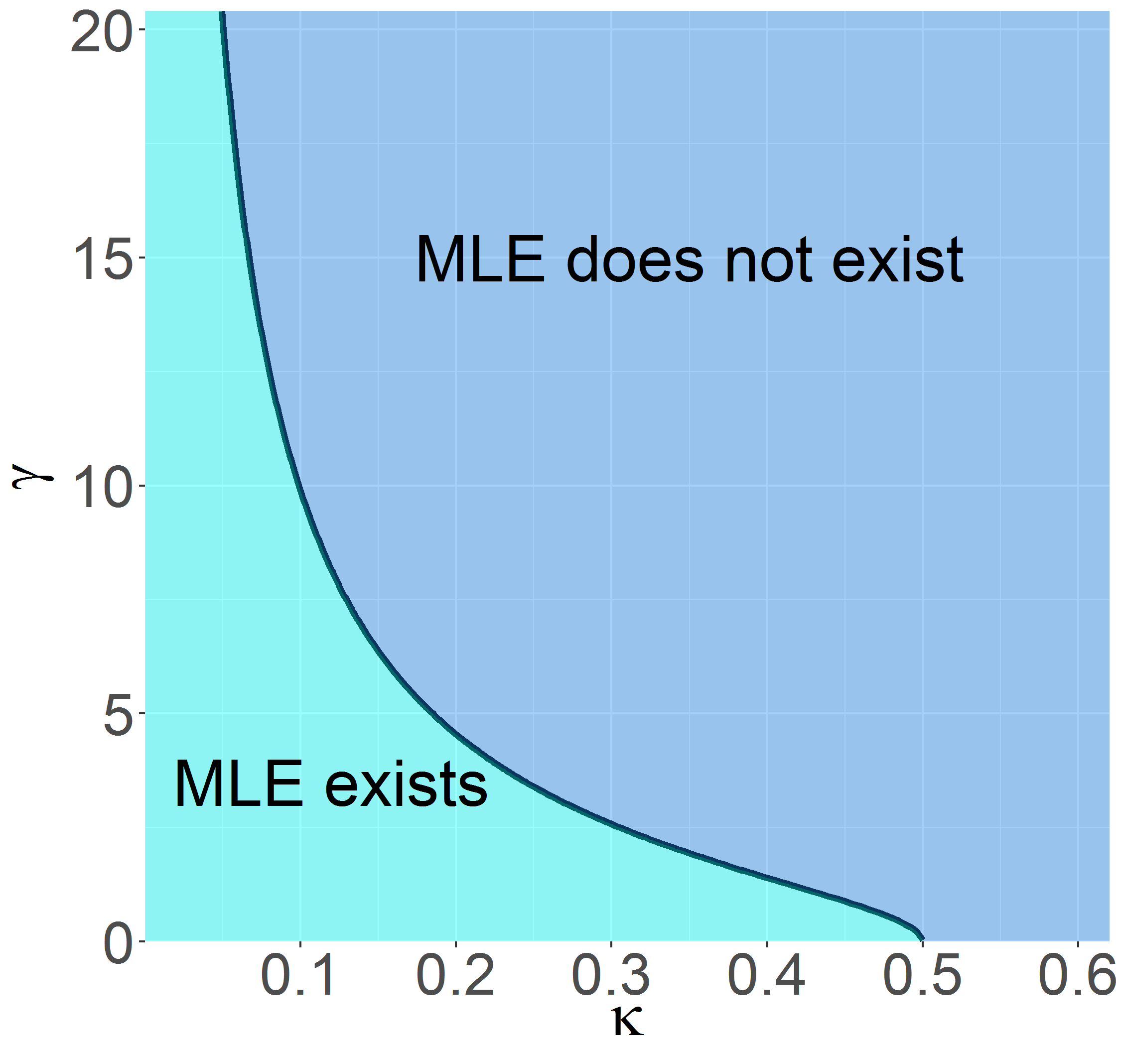
Figure 1: Boundary curve $\kappa\mapsto g_{\text{MLE}}(\kappa)$ separating the regions where the MLE asymptotically exists and where it does not [9, Figure 1(a)].

An important issue in logistic regression is that the MLE does not always exist. In fact, the MLE exists if and only if the cases (the points $\boldsymbol{x}_{i}$ for which $y_{i}=1$) and controls (those for which $y_{i}=-1$) cannot be linearly separated; linear separation here means that there is a hyperplane such that all the cases are on one side of the plane and all the controls on the other.

When both $n$ and $p$ are large, whether such a separating hyperplane exists depends only on the dimensionality $\kappa$ and the overall signal strength $\gamma$. In the asymptotic setting described above, [9, Theorem 1] demonstrated a phase transition phenomenon: there is a curve $\gamma=g_{\text{MLE}}(\kappa)$ in the $(\kappa,\gamma)$ plane that separates the region where the MLE exists from that where it does not, see Figure 1. Formally,

$$\gamma>g_{\mathrm{MLE}}(\kappa)\implies\lim_{n,p\to\infty}\operatorname{\mathbb{P}}(\mathrm{MLE\>exists})\to 0,$$

$$\gamma<g_{\mathrm{MLE}}(\kappa)\implies\lim_{n,p\to\infty}\operatorname{\mathbb{P}}(\mathrm{MLE\>exists})\to 1.$$

It is noteworthy that the phase-transition diagram only depends on whether $\gamma>g_{\text{MLE}}(\kappa)$ and, therefore, does not depend on the details of the covariance $\boldsymbol{\Sigma}$ of the covariates. Since we are interested in the distribution of the MLE, we shall consider values of the dimensionality parameter $\kappa$ and signal strength $\gamma$ in the light blue region from Figure 1.

3.2 Finite-dimensional marginals of the MLE

We begin by establishing the asymptotic behavior of the random variables $\alpha(n)$ and $\sigma(n)$, introduced in (2.7). These limits will play a key role in the distribution of the MLE.

Lemma 3.1.

Consider a sequence of logistic models with covariates drawn i.i.d. from $\mathcal{N}(\boldsymbol{0},\boldsymbol{I}_{p})$ and regression vectors $\boldsymbol{\theta}$ satisfying $\lim_{n\to\infty}\|\boldsymbol{\theta}\|^{2}\,\to\,\gamma^{2}$. Let $\hat{\boldsymbol{\theta}}$ be the MLE and define $\alpha(n)$ and $\sigma(n)$ as in (2.7). Then, if $(\kappa,\gamma)$ lies in the region where the MLE exists asymptotically, we have that

$$\alpha(n)\,\,\stackrel{{\scriptstyle\mathrm{a.s.}}}{{\longrightarrow}}\,\,\alpha_{\star}\qquad\mathrm{and}\qquad\sigma(n)^{2}\,\,\stackrel{{\scriptstyle\mathrm{a.s.}}}{{\longrightarrow}}\,\,\kappa\sigma_{\star}^{2},$$ (3.3)

where $\alpha_{\star}$ and $\sigma_{\star}$ are numerical constants that only depend on $\kappa$ and $\gamma$.

We defer the proof to the supplementary material [46, Section A]; here, we explain where the parameters $(\alpha_{\star},\sigma_{\star})$ come from. Along with an additional parameter $\lambda_{\star}$, the triple $(\alpha_{\star},\sigma_{\star},\lambda_{\star})$ is the unique solution to the system of equations parameterized by $(\kappa,\gamma)$ in three variables $(\alpha,\sigma,\lambda)$ given by

$$\begin{dcases}\sigma^{2}&=\frac{1}{\kappa^{2}}\mathbb{E}\left[2\rho^{\prime}(Q_{1})(\lambda\rho^{\prime}(\mathsf{prox}_{\lambda\rho}(Q_{2})))^{2}\right]\\ 0&=\mathbb{E}\left[\rho^{\prime}(Q_{1})Q_{1}\lambda\rho^{\prime}(\mathsf{prox}_{\lambda\rho}(Q_{2}))\right]\\ 1-\kappa&=\mathbb{E}\left[\frac{2\rho^{\prime}(Q_{1})}{1+\lambda\rho^{\prime\prime}(\mathsf{prox}_{\lambda\rho}(Q_{2}))}\right],\end{dcases}$$ (3.4)

where $(Q_{1},Q_{2})$ is a bivariate normal variable with mean $\boldsymbol{0}$ and covariance

$$\boldsymbol{\Sigma}(\alpha,\sigma)=\left[\begin{matrix}\gamma^{2}&-\alpha\gamma^{2}\\ -\alpha\gamma^{2}&\alpha^{2}\gamma^{2}+\kappa\sigma^{2}\end{matrix}\right].$$

Above, the proximal operator is defined as

$$\mathsf{prox}_{\lambda\rho}(z)=\arg\min_{t\in\mathbb{R}}\left\{\lambda\rho(t)+\frac{1}{2}(t-z)^{2}\right\},$$

where $\rho(t)=\log(1+e^{t})$. This system of equations can be rigorously derived from the generalized approximate message passing algorithm [32, 20], or by analyzing the auxiliary optimization problem [34]. They can also be heuristically understood with an argument similar to that in [14]; we defer to [38] for a complete discussion. The important point here is that in the region where the MLE exists, the system (3.4) has a unique solution. Lemma 3.1 contributes novel insights by interpreting $\alpha_{\star},\sigma_{\star}$ through the lens of the finite sample quantities $\alpha(n),\sigma(n)$, which proves crucial for establishing Theorem 3.1.

We are now in a position to describe the asymptotic behavior of the MLE. The proof is deferred to the supplementary material [46, Section A].

Theorem 3.1.

Consider a logistic model with covariates $\boldsymbol{x}_{i}$ drawn i.i.d. from $\mathcal{N}(\boldsymbol{0},\boldsymbol{\Sigma}(n))$ and assume we are in the $(\kappa,\gamma)$ region where the MLE exists asymptotically. Then for every coordinate whose regression coefficient satisfies $\sqrt{n}\tau_{j}\beta_{j}=O(1)$,

$$\frac{\sqrt{n}(\hat{\beta}_{j}-\alpha_{\star}\beta_{j})}{\sigma_{\star}/\tau_{j}}\,\stackrel{{\scriptstyle\mathrm{d}}}{{\longrightarrow}}\,\mathcal{N}(0,1).$$ (3.5)

Above $\tau^{2}_{j}=\operatorname{Var}(x_{i,j}\,|\,\boldsymbol{x}_{i,-j})$ is the conditional variance of $x_{i,j}$ given all the other covariates. More generally, for any sequence of deterministic unit normed vectors $\boldsymbol{v}(n)$ with $\sqrt{n}\tau(\boldsymbol{v})\boldsymbol{v}(n)^{\top}\boldsymbol{\beta}(n)=O(1)$, we have that

$$\frac{\sqrt{n}\boldsymbol{v}^{\top}(\hat{\boldsymbol{\beta}}-\alpha_{\star}\boldsymbol{\beta})}{\sigma_{\star}/\tau(\boldsymbol{v})}\,\stackrel{{\scriptstyle\mathrm{d}}}{{\longrightarrow}}\,\mathcal{N}(0,1).$$ (3.6)

Here $\tau(\boldsymbol{v})$ is given by

$$\tau^{2}(\boldsymbol{v})=\mathrm{Var}(\boldsymbol{v}^{\top}\boldsymbol{x}_{i}|P_{\boldsymbol{v}^{\perp}}\boldsymbol{x}_{i})=\left(\boldsymbol{v}^{\top}\boldsymbol{\Theta}(n)\boldsymbol{v}\right)^{-1},$$

where $\boldsymbol{\Theta}(n)$ equals the precision matrix $\boldsymbol{\Sigma}(n)^{-1}$. A consequence is this: consider a finite set of coordinates $\mathcal{S}\subset\{1,\ldots,p\}$ obeying $\sqrt{n}({\boldsymbol{\beta}_{\mathcal{S}}^{\top}\boldsymbol{\Theta}_{\mathcal{S}}^{-1}\boldsymbol{\beta}_{\mathcal{S}}})^{\frac{1}{2}}=O(1)$. Then

$$\frac{\sqrt{n}\boldsymbol{\Theta}_{\mathcal{S}}^{-1/2}(\hat{\boldsymbol{\beta}}_{\mathcal{S}}-\alpha_{\star}\boldsymbol{\beta}_{\mathcal{S}})}{\sigma_{\star}}\,\,\stackrel{{\scriptstyle\mathrm{d}}}{{\longrightarrow}}\,\,\mathcal{N}(\boldsymbol{0},\boldsymbol{I}_{|\mathcal{S}|}).$$ (3.7)

Above $\boldsymbol{\beta}_{\mathcal{S}}$ is the slice of $\boldsymbol{\beta}$ with entries in $\mathcal{S}$ and, similarly, $\boldsymbol{\Theta}_{\mathcal{S}}$ is the slice of the precision matrix $\boldsymbol{\Theta}$ with rows and columns in $\mathcal{S}$.

Returning to the Introduction, we now see that the behavior of the MLE is different from that implied by the classical textbook result, which states that

$$\sqrt{n}(\hat{\boldsymbol{\beta}}-\boldsymbol{\beta})\,\,\stackrel{{\scriptstyle\mathrm{d}}}{{\longrightarrow}}\,\,\mathcal{N}(0,\mathcal{I}^{-1}_{\beta}).$$

We also see that Theorem 3.1 extends [38, Theorem 3] in multiple directions. Indeed, this prior work assumed standardized and independent covariates (i.e. $\boldsymbol{\Sigma}=\boldsymbol{I}$)—implying that $\tau_{j}^{2}=1$—and established $\sqrt{n}\hat{\beta}_{j}/\sigma_{\star}\stackrel{{\scriptstyle\mathrm{d}}}{{\longrightarrow}}\mathcal{N}(0,1)$ only in the special case $\beta_{j}=0$.

3.2.1 Finite sample accuracy

We study the finite sample accuracy of Theorem 3.1 through numerical examples. We consider an experiment with a fixed number of observations set to $n=4,000$ and a number of variables set to $p=800$ so that $\kappa=0.2$. We set the signal strength to $\gamma^{2}=5$. (For this problem size, the asymptotic result for null variables has been observed to be very accurate when the covariates are independent [38].)

We sample the covariates such that the covariance matrix is the correlation matrix from an AR(1) model with parameter $\rho=0.5$, i.e. $\Sigma_{ij}=\rho^{|i-j|}$. We then randomly sample half of the coefficients to be non-nulls, with equal and positive magnitudes, chosen to attain the desired signal strength $\boldsymbol{\beta}^{\top}\boldsymbol{\Sigma}\boldsymbol{\beta}=5$. For a given non-null coordinate $\beta_{j}$, we calculate the centered and scaled MLE $T_{j}$ (1.2), and repeat the experiment $B=100,000$ times. Figure 2 shows a qqplot of the empirical distribution of $T_{j}$ versus the standard normal distribution. Observe that the quantiles align perfectly, demonstrating the accuracy of (3.5).

We further examine the empirical accuracy of (3.5) through the lens of confidence intervals and finite sample coverage. Theorem 3.1 suggests that if $z_{(1-\alpha/2)}$ is the $(1-\alpha/2)$th quantile of a standard normal variable, $\beta_{j}$ should lie within the interval

$$\left[\frac{1}{\alpha_{\star}}\left(\hat{\beta}_{j}-\frac{\sigma_{\star}}{\sqrt{n}\tau_{j}}z_{(1-\alpha/2)}\right),\frac{1}{\alpha_{\star}}\left(\hat{\beta}_{j}+\frac{\sigma_{\star}}{\sqrt{n}\tau_{j}}z_{(1-\alpha/2)}\right)\right]$$ (3.8)

about $(1-\alpha)B$ times. Table 1 shows the proportion of experiments in which $\beta_{j}$ is covered by (3.8) for different choices of the confidence level $(1-\alpha)$, along with the respective standard errors. For every confidence level, the empirical coverage proportion lies extremely close to the corresponding target.

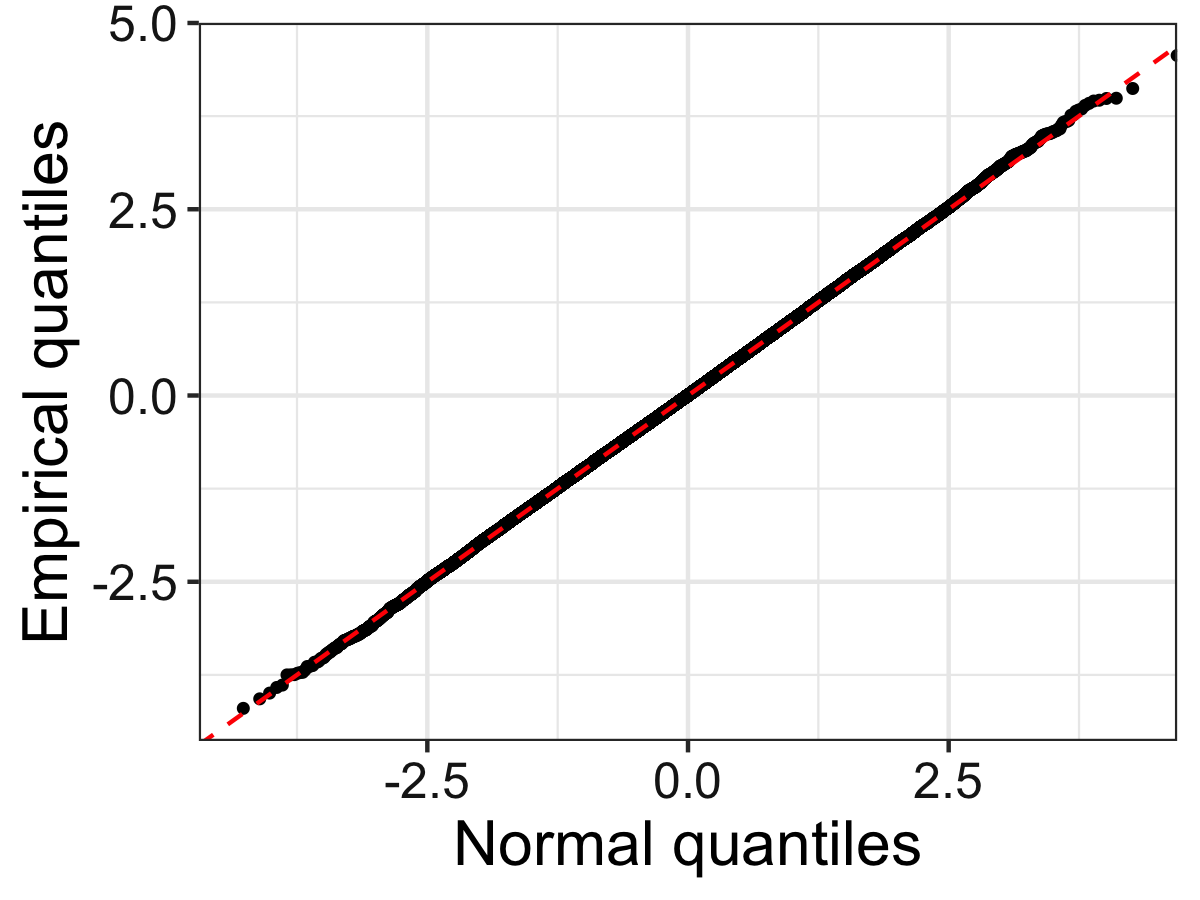
Figure 2: Quantiles of the empirical distribution of an appropriately centered and scaled MLE coordinate versus standard normal quantiles.

Table 1: Coverage proportion of a single variable. Each cell reports the proportion of times $\beta_{j}$ falls within (3.8), calculated over $B=100,000$ repetitions; the standard errors are provided as well.

Nominal coverage
$100(1-\alpha)$	99	98	95	90	80
Empirical coverage	98.97	97.96	94.99	89.88	79.88
Standard error	0.03	0.04	0.07	0.10	0.13

3.2.2 Condition on the regression coefficients

In this section, we conduct simulations to investigate to what extent the condition on the magnitude of $\beta_{j}$ in Theorem 3.1 may be relaxed. We vary the magnitude of the non-null coefficients $\beta_{j}$ by choosing $\beta_{j}$ such that $\tau_{j}\beta_{j}/\gamma\in\{0.15,0.3,0.5\}$ (so that $\sqrt{n}\tau_{j}\beta_{j}$ is large). We report the variance of a single MLE coordinate in $B=10,000$ repeated experiments (Figure 3). The observed biases range from 1.450 to 1.461 in the simulations and do not show a pattern. In this example, we set $\kappa=0.2$, $\gamma=2$ and use the same covariance matrix as in the last paragraph. The theoretical standard deviation of $\hat{\beta}_{j}$ is thus 5.65 (dashed line). We observe that our theory works well when $\tau_{j}\beta_{j}/\gamma\leq 0.15$, because the empirical standard error is close to the theoretical prediction and the MLE is approximately Gaussian (Figure 3(b)). However, the standard error of the MLE increases as $\beta_{j}$ increases. At $\tau_{j}\beta_{j}/\gamma=0.5$, for instance, the observed standard error when $n=4000$ is 7.71, which is 36% percent larger than the theoretical standard deviation. We also observe that for a fixed $\gamma$ and $\kappa$, the standard error slightly decreases as $n$ increases, suggesting that the theory becomes more accurate at larger $n$ if $\tau_{j}\beta_{j}/\gamma\lesssim 0.15$.

Now that we have reasons to believe the theory holds for $\tau_{j}\beta_{j}$ that is not vanishing, we study a possible path to a sharper statement. Theorem 3.1 requires the condition $\sqrt{n}\tau_{j}\beta_{j}=O(1)$ to ensure that $\sqrt{n}(\alpha(n)-\alpha_{\star})\tau_{j}\beta_{j}=o(1)$. (See the proof in [46, Section A].) We thus study the behavior of the random variable $\sqrt{n}(\alpha(n)-\alpha_{\star})$ and compute its standard deviation. We use the same covariance matrix as before and set half of the variables to be non-nulls. We compute $\alpha(n)$ as $\alpha(n)=\hat{\beta}^{\top}\Sigma\beta/\gamma^{2},$ and report

$$\widehat{\mathrm{sd}}(\sqrt{n}(\alpha(n)-\alpha_{\star}))=\left(\frac{1}{m}\sum_{i=1}^{m}\left[\sqrt{n}(\alpha_{i}(n)-\alpha_{\star})\right]^{2}\right)^{1/2}$$ (3.9)

over $m=10,000$ repetitions (Figure 4). We observe that while the standard deviations differ for varied choices of $\kappa$ and $\gamma$, they slightly decrease as $n$ increases and approach a constant asymptote. This suggests that $\sqrt{n}(\alpha(n)-\alpha_{\star})=O_{P}(1)$ and the condition may be relaxed to $\tau_{j}\beta_{j}=o(1)$. We do not expect that this latter condition can be relaxed further. To see this, note that this condition $\tau_{j}\beta_{j}=o(1)$ was required for [38, Theorem 2], since this earlier result holds in the setting where the empirical distribution of $\beta$ converges weakly to a distribution with finite second moment. In the setting of [38], $\tau_{j}=1/\sqrt{n}$ and therefore, their condition implies that $\tau_{j}\beta_{j}=o(1)$ for every coordinate.

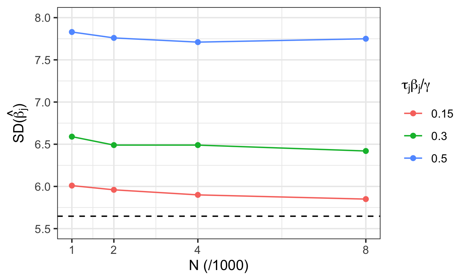
(a)

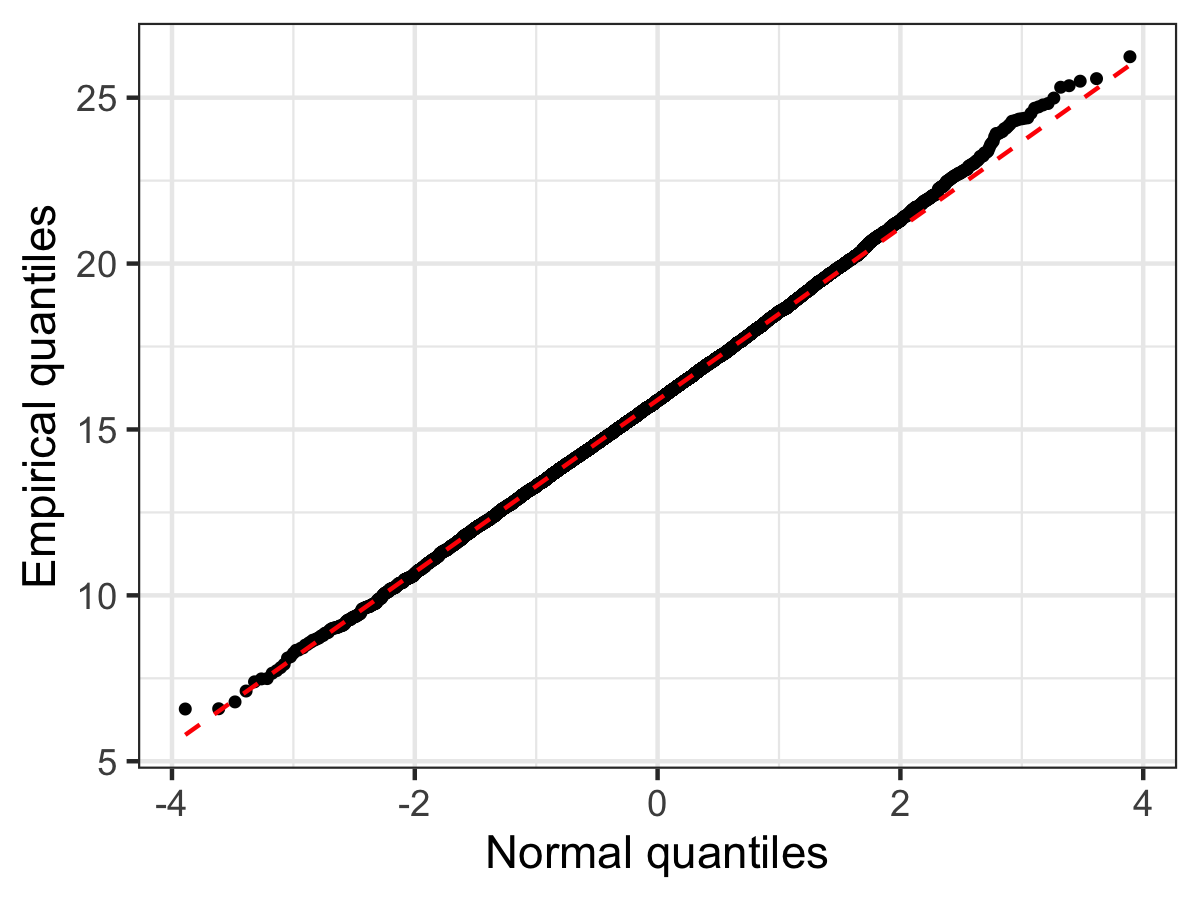
(b)

Figure 3: (a) Standard deviation of a single MLE $\hat{\beta}_{j}$ versus the sample size $n$ (shown on the $x$-axis as $n/1000$) when size of the coefficient $\beta_{j}$ varies at $\tau_{j}\beta_{j}/\gamma\in\{0.15,0.3,0.5\}$. $\mathrm{SD}(\hat{\beta}_{j})$ is larger than than theoretical value (dashed line) when $\beta_{j}$ is large. The standard deviations are calculated from $B=10,000$ repetitions. (b) Normal quantile plot for the non-null variable with $\tau_{j}\beta_{j}/\gamma=0.15$ and $n=4000$ in Figure (a).

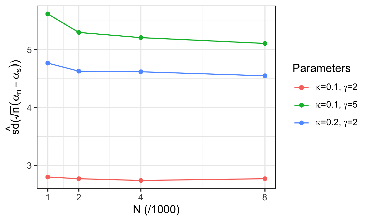
Figure 4: Plot of $\widehat{\mathrm{sd}}(\sqrt{n}(\alpha(n)-\alpha_{\star}))$ (see Eqn. (3.9)) versus the sample size $n$ different parameters $\kappa$ and $\gamma$.

3.3 The empirical distribution of all MLE coordinates (single experiment)

The preceding section tells us about the finite-dimensional marginals of the MLE, e.g. about the distribution of a given coordinate $\hat{\beta}_{j}$ when we repeat experiments. We now turn to a different type of asymptotics and characterize the limiting empirical distribution of all the coordinates calculated from a single experiment.

Theorem 3.2.

Let $c(n)=\lambda_{\max}(\boldsymbol{\Sigma}(n))/\lambda_{\min}(\boldsymbol{\Sigma}(n))$ be the condition number of $\boldsymbol{\Sigma}(n)$. Assume that $\limsup_{n\to\infty}\,c(n)<\infty$, and that $(\kappa,\gamma)$ lies in the region where the MLE exists asymptotically. Then the empirical cumulative distribution function of the rescaled MLE (1.2) converges pointwise to that of a standard normal distribution, namely, for each $t\in\mathbb{R}$,

$$\frac{1}{p}\sum_{i=1}^{p}\mathbb{I}\left\{T_{j}\leq t\right\}\stackrel{{\scriptstyle\mathrm{P}}}{{\longrightarrow}}\Phi(t).$$ (3.10)

As explained in the Introduction, this says that empirical averages of functionals of the marginals have a limit (1.5). By [46, Corollary B.2], this implies that the empirical distribution of $\boldsymbol{T}$ converges weakly to a standard Gaussian, in probability.

The statement above can be extended to general testing functions (the proof is provided in the supplementary material [46, Section C]):

Theorem 3.3.

Consider any pseudo-Lipschitz function of order 2 and suppose the conditions of Theorem 3.1 hold. Further, assume that the empirical distribution sequence $\sum_{j=1}^{p}\delta_{\sqrt{n}\tau_{j}\beta_{j}}/p$ converges weakly to a distribution $\Pi$ with finite second moment and that $\frac{1}{p}\sum_{j=1}^{p}n\tau_{j}^{2}\beta_{j}^{2}\stackrel{{\scriptstyle p}}{{\longrightarrow}}\mathbb{E}\left[\eta^{2}\right]$ for $\eta\sim\Pi$, then

$$\frac{1}{p}\sum_{i=1}^{p}\psi(\sqrt{n}\tau_{j}(\hat{\beta}_{j}-\alpha_{\star}\beta_{j}),\sqrt{n}\tau_{j}\beta_{j})\stackrel{{\scriptstyle P}}{{\longrightarrow}}\mathbb{E}\left[\psi(\sigma_{\star}Z,\eta)\right].$$ (3.11)

In the remainder of this section, we study the empirical accuracy of Theorem 3.2 in finite samples through some simulated examples.

The nature of this result is similar to [38, Theorem 2]. However, the techniques from [38] cannot be applied here. To prove Theorem 3.2, we connect the rescaled MLE vector $\boldsymbol{T}$ with a correlated Gaussian vector through a stochastic representation result, similar in spirit to Lemma 2.1. This is done in [46, Proposition B.1] and [46, Corollary B.1]. The rest of the proof focuses on analyzing this representation, see [46, Section B].

3.3.1 Finite sample accuracy

We consider an experiment with dimensions $n$ and $p$ the same as that for Figure 2, and the regression vector sampled similarly. According to (3.10), about $(1-\alpha)$ of all the $\beta_{j}$’s should lie within the corresponding intervals (3.8).

Table 2 shows the proportion of $\beta_{j}$’s covered by these intervals for a few commonly used confidence levels $(1-\alpha)$. The proportions are as predicted for each of the confidence levels, and every covariance we simulated from.

The four columns in Table 2 correspond to different covariance matrices; they include a random correlation matrix (details are given below), a correlation matrix from an AR(1) model whose parameter is either set to $\rho=0.8$ or $\rho=0.5$, and a covariance matrix set to be the identity. The random correlation matrix is sampled as follows: we randomly pick an orthogonal matrix $\boldsymbol{U}$, and eigenvalues $\lambda_{1},\dots,\lambda_{p}$ i.i.d. from a chi-squared distribution with 10 degrees of freedom. We then form a positive definite matrix $\boldsymbol{B}=\boldsymbol{U}^{\top}\boldsymbol{\Lambda}\boldsymbol{U}$ from these eigenvalues, where $\boldsymbol{\Lambda}=\mathrm{diag}(\lambda_{1},\dots,\lambda_{p})$. $\boldsymbol{\Sigma}$ is the correlation matrix obtained from $\boldsymbol{B}$ by scaling the variables to have unit variance.

Table 2: Each cell reports the proportion of all the variables in each run falling within the corresponding intervals from (3.8), averaged over $B=100,000$ repetitions; the standard deviation is given between parentheses.

Nominal coverage
$100(1-\alpha)$	Random	$\rho=0.8$	$\rho=0.5$	Identity
99	99.178 (0.002)	99.195 (0.002)	99.187 (0.002)	99.175 (0.002)
98	97.873 (0.003)	97.908 (0.003)	97.890 (0.003)	97.865 (0.003)
95	94.826 (0.005)	94.884 (0.005)	94.857 (0.005)	94.811 (0.005)
90	89.798 (0.007)	89.883 (0.007)	89.847 (0.007)	89.780 (0.007)
80	79.784 (0.009)	79.896 (0.009)	79.837 (0.009)	79.751 (0.009)

4 The distribution of the LRT

Lastly, we study the distribution of the log-likelihood ratio (LLR) test statistic

$$\operatorname{LLR}_{j}=\max_{\boldsymbol{b}}\ell(\boldsymbol{b};\boldsymbol{X},\boldsymbol{y})-\max_{\boldsymbol{b}:\>{b}_{j}=0}\ell(\boldsymbol{b};\boldsymbol{X},\boldsymbol{y}),$$ (4.1)

which is routinely used to test whether the $j$th variable is in the model or not; i. e. whether $\beta_{j}=0$ or not.

Theorem 4.1.

Assume that we are in the $(\kappa,\gamma)$ region where the MLE exists asymptotically. Then under the null (i.e. $\beta_{j}=0$),

$$2\operatorname{LLR}_{j}\,\,\stackrel{{\scriptstyle\mathrm{d}}}{{\longrightarrow}}\,\,\frac{\kappa\sigma_{\star}^{2}}{\lambda_{\star}}\chi^{2}_{1}.$$

Further, for every finite $\ell$, twice the LLR for testing $\ell$ null hypotheses $\beta_{j_{1}}=\dots=\beta_{j_{\ell}}=0$ is asymptotically distributed as $(\kappa\sigma_{\star}^{2}/\lambda_{\star})\,\,\chi^{2}_{\ell}$.

Invoking results from Section 2.1, we will show that this is a rather straightforward extension of [38, Theorem 4], which deals with independent covariates, see also [37, Theorem 1]. Choosing $\boldsymbol{L}$ to be the same as in (2.4) after permuting $\beta_{j}$ to be the last variable and setting $\boldsymbol{b}^{\prime}=\boldsymbol{L}^{\top}\boldsymbol{b}$ tell us that $b^{\prime}_{j}=0$ if and only if $b_{j}=0$. Hence, $\mathrm{LLR_{j}}$ reduces to

$$\operatorname{LLR}_{j} =\max_{\boldsymbol{b}}\ell(\boldsymbol{L}^{\top}\boldsymbol{b};\boldsymbol{X}\boldsymbol{L}^{-\top},\boldsymbol{y})-\max_{\boldsymbol{b}:b_{j}=0}\ell(\boldsymbol{L}^{\top}\boldsymbol{b};\boldsymbol{X}\boldsymbol{L}^{-\top},\boldsymbol{y})$$ (4.2)

$$=\max_{\boldsymbol{b}^{\prime}}\ell(\boldsymbol{b}^{\prime};\boldsymbol{X}\boldsymbol{L}^{-\top},\boldsymbol{y})-\max_{\boldsymbol{b}^{\prime}:b^{\prime}_{j}=0}\ell(\boldsymbol{b}^{\prime};\boldsymbol{X}\boldsymbol{L}^{-\top},\boldsymbol{y}),$$ (4.3)

which is the log-likelihood ratio statistic in a model with covariates drawn i.i.d. from $\mathcal{N}(\boldsymbol{0},\boldsymbol{I}_{p})$ and regression coefficient given by $\boldsymbol{\theta}=\boldsymbol{L}^{\top}\boldsymbol{\beta}$. This in turn satisfies $\theta_{j}=0$ if and only if $\beta_{j}=0$ so that we can think of the LLR above as testing $\theta_{j}=0$. Consequently, the asymptotic distribution is the same as that given in [38, Theorem 4] with $\gamma^{2}=\lim_{n\rightarrow\infty}\|\boldsymbol{\theta}\|^{2}=\lim_{n\rightarrow\infty}\boldsymbol{\beta}^{\top}\boldsymbol{\Sigma}\boldsymbol{\beta}$. The equality of the likelihood ratios implies that to study the finite sample accuracy of Theorem 4.1, we may just as well assume we have independent covariates; hence, we refer the readers to [38] for empirical results detailing the quality of the rescaled chi-square approximation in finite samples.

5 Accuracy with estimated parameters

In practice, the signal strength $\gamma^{2}$ and conditional variance $\tau_{j}^{2}$ are typically not known a priori. In this section, we plug in estimates of these quantities and investigate their empirical performance. We focus on testing a null variable and constructing confidence intervals.

The parameters are the same as in Section 3.2. In brief, we set $n=4,000$, $p=800$ (so that $\kappa=0.2$), and $\gamma^{2}=5$. The covariates follow an AR(1) model with $\rho=0.5$ and $\Sigma_{jj}=1$.

5.1 Estimating parameters

We here explain how to estimate the signal strength $\gamma^{2}$ and conditional variance $\tau_{j}^{2}$ needed to describe the distribution of the LLR and MLE.

To estimate the signal strength, we use the ProbeFrontier method introduced in [38]. As we have seen in Section 3.1, for each $\gamma$, there is a corresponding problem dimension $\kappa(\gamma)$ on the phase transition curve, see Figure 1: once $\kappa>\kappa(\gamma)$, the MLE no longer exists asymptotically [9]. The ProbeFrontier method searches for the smallest $\kappa$ such that the MLE ceases to exist by sub-sampling observations. Once we obtain $\hat{\gamma}$, we set $(\hat{\alpha},\hat{\sigma},\hat{\lambda})$ to be the solution to the system of equations with parameters $(\kappa,\hat{\gamma})$. Because the ProbeFrontier method only checks whether the points are separable, the quality of the estimate $\hat{\gamma}$ does not depend upon whether the covariates are independent or not. We therefore expect good performance across the board.

As to the conditional variance, since the covariates are Gaussian, it can be estimated by a simple linear regression. Let $\boldsymbol{X}_{\bullet,-j}$ be the data matrix without the $j$th column, and consider the residual sum of squares $\text{RSS}_{j}$ obtained by regressing the $j$th column $\boldsymbol{X}_{\bullet,j}$ onto $\boldsymbol{X}_{\bullet,-j}$. Then

$$\text{RSS}_{j}\,\,\sim{\tau_{j}^{2}}\,\,\chi^{2}_{n-p+1}.$$

Hence,

$$\hat{\tau}_{j}^{2}=\frac{\text{RSS}_{j}/n}{1-\kappa}$$ (5.1)

is nearly unbiased for $\tau_{j}^{2}$.

In our example, the covariates follow an AR(1) model and there is a natural estimate of $\rho$ by maximum likelihood. This yields an estimated covariance matrix $\hat{\boldsymbol{\Sigma}}(\hat{\rho})$ parameterized by $\hat{\rho}$, which we then use to estimate the conditional variance $\hat{\tau}^{2}_{j}(\hat{\rho})$. Below, we use both the nonparametric estimates $\hat{\tau}_{j}$ and parametric estimates $\hat{\tau}_{j}(\hat{\rho})$.

5.2 Empirical performance of a $t$-test

Imagine we want to use Theorem 3.1 to calibrate a test to decide whether $\beta_{j}=0$ or not. After plugging in estimated parameters, a p-value for a two-sided test takes the form

$$\hat{p}_{j}=2\bar{\Phi}(\sqrt{n}\hat{\tau}_{j}|\hat{\beta}_{j}|/\hat{\sigma}),$$ (5.2)

where $\bar{\Phi}(t)=\mathbb{P}(\mathcal{N}(0,1)>t)$. In Table 3, we report the proportion of p-values calculated from (5.2), below some common cutoffs. To control type-I errors, the proportion of p-values below 10% should be at most about 10% and similarly for any other level. The p-values computed from true parameters show a correct behavior, as expected. If we use estimated parameters, the p-values are also accurate and are as good as those obtained from true parameters. In comparison, p-values from classical theory are far from correct, as shown in Column 4.

Table 3: Empirical performance of a $t$-test from (5.2). Each cell reports the p-value probability and its standard error (in parentheses) estimated over $B=10,000$ repetitions. The first two columns use ProbeFrontier to estimate the problem parameter $\hat{\sigma}$, and the two estimates of conditional variance from Section 5.1. The third column assumes knowledge of the signal-to-noise parameter $\gamma$. The last column uses the normal approximation from R.

	1	2	3	4
	$(\hat{\tau},\hat{\sigma})$	$(\hat{\tau}(\hat{\rho}),\hat{\sigma})$	$(\tau,\sigma_{\star})$	Classical
$\mathbb{P}(\text{P-value}\leq 10\%)$	10.09% (0.30%)	10.14% (0.30%)	10.22% (0.30%)	17.80% (0.38%)
$\mathbb{P}(\text{P-value}\leq 5\%)$	5.20% (0.22%)	5.23% (0.22%)	5.24% (0.22%)	10.73% (0.31%)
$\mathbb{P}(\text{P-value}\leq 1\%)$	1.16% (0.11%)	1.22% (0.11%)	1.33% (0.11%)	3.72% (0.19%)
$\mathbb{P}(\text{P-value}\leq 0.5\%)$	0.68% (0.08%)	0.70% (0.08%)	0.74% (0.08%)	2.43% (0.15%)

5.3 Coverage proportion

We proceed to check whether the confidence intervals constructed from the estimated parameters

$$\left[\frac{1}{\hat{\alpha}}\left(\hat{\beta}_{j}-\frac{\hat{\sigma}}{\sqrt{n}\hat{\tau}_{j}}z_{(1-\alpha/2)}\right),\frac{1}{\hat{\alpha}}\left(\hat{\beta}_{j}+\frac{\hat{\sigma}}{\sqrt{n}\hat{\tau}_{j}}z_{(1-\alpha/2)}\right)\right]$$ (5.3)

achieve the desired coverage property.

Table 4: Coverage proportion of a single variable. Each cell reports the proportion of times a variable $\beta_{j}$ is covered by the corresponding confidence interval from (5.3), calculated over $B=10,000$ repetitions; we chose the variable to be the same null coordinate as in Section 5.2. The standard errors are given between parentheses. The first two columns use estimated parameters, and the last one uses the true parameters.

Nominal coverage	1	2	3
$100(1-\alpha)$	$(\hat{\tau},\hat{\sigma})$	$(\hat{\tau}(\hat{\rho}),\hat{\sigma})$	$(\tau,\sigma_{\star})$
99.5	99.32 (0.08)	99.30 (0.08)	99.26 (0.09)
99	98.84 (0.11)	98.78 (0.11)	98.67 (0.11)
95	94.80 (0.22)	94.77 (0.22)	94.76 (0.22)
90	89.91 (0.30)	89.86 (0.30)	89.78 (0.30)

Table 5: Proportion of variables inside the confidence intervals (5.3). Each cell reports the proportion of all the variables in each run falling within the corresponding confidence intervals from (5.3), averaged over $B=10,000$ repetitions (standard errors in parentheses). The first two columns use estimated parameters, and the last one uses the true parameters.

Nominal coverage	1	2	3
$100(1-\alpha)$	$(\hat{\tau},\hat{\sigma})$	$(\hat{\tau}(\hat{\rho}),\hat{\sigma})$	$(\tau,\sigma_{\star})$
98	97.96 (0.01)	97.95 (0.01)	97.85 (0.01)
95	95.01 (0.01)	95.00 (0.01)	94.85 (0.02)
90	89.92 (0.02)	89.91 (0.02)	89.72 (0.02)
80	79.99 (0.02)	79.99 (0.02)	79.77 (0.03)

We first test this in the context of Theorem 3.1, in particular (3.5). Table 4 reports the proportion of times a single coordinate lies in the corresponding confidence interval from (5.3). We observe that the coverage proportions are close to the respective targets, even with the estimated parameters.

Moving on, we study the accuracy of the estimated parameters in light of Theorem 3.2. This differs from our previous calculation: Table 4 focuses on whether a single coordinate is covered, but now we compute the proportion of all the $p=800$ variables falling within the respective confidence intervals from (5.3), in each single experiment. We report the mean of these proportions (Table 5), computed across 10,000 repetitions. Ideally, the proportion should be about the nominal coverage and this is what we observe.

5.4 Empirical performance of the LRT

Lastly, we examine p-values for the LRT when the signal strength $\gamma^{2}$ is unknown. The p-values take the form

$$\hat{p}_{j}=\operatorname{\mathbb{P}}\left(\chi^{2}_{1}\geq\frac{\hat{\lambda}}{\kappa\hat{\sigma}^{2}}\;2\mathrm{LLR}_{j}\right)$$ (5.4)

once we plug in estimated values for $\lambda_{\star}$ and $\sigma_{\star}$. Table 6 displays the proportion of p-values below some common cutoffs for the same null coordinate as in Table 3. Again, classical theory yields a gross inflation of the proportion of p-values in the lower tail. In contrast, p-values from either estimated or true parameters display the correct behavior.

Table 6: Empirical performance of the LRT. Each cell reports the p-value probability and its standard error (in parentheses) estimated over $B=10,000$ repetitions. The first column uses ProbeFrontier estimated factor $\hat{\lambda}/\kappa\hat{\sigma}^{2}$ whereas the second uses $\lambda_{\star}/\kappa\sigma_{\star}^{2}$. The last column displays the results from classical theory.

	Estimated	True	Classical
$\mathbb{P}(\text{P-value}\leq 10\%)$	10.04% (0.30%)	10.06% (0.30%)	17.86% (0.38%)
$\mathbb{P}(\text{P-value}\leq 5\%)$	5.19% (0.22%)	5.25% (0.22%)	10.76% (0.31%)
$\mathbb{P}(\text{P-value}\leq 1\%)$	1.17 % (0.11%)	1.18% (0.11%)	3.75% (0.19%)
$\mathbb{P}(\text{P-value}\leq 0.5\%)$	0.68% (0.08%)	0.69% (0.08%)	2.49% (0.15%)

6 A sub-Gaussian example

Our model assumes that the covariates arise from a multivariate normal distribution. As in [38, Section 4.g], however, we expect that our results apply to a broad class of covariate distributions, in particular, when they have sufficiently light tails. To test this, we consider a logistic regression problem with covariates drawn from a sub-Gaussian distribution that is inspired by genetic studies, and examine the accuracy of null p-values and confidence intervals proposed in this paper.

Since the signal strength $\gamma^{2}$ and conditional variances $\tau_{j}^{2}$ are unknown in practice, we use throughout the ProbeFrontier method and (5.1) to obtain accurate estimates.

6.1 Model setting

In genome-wide association studies (GWAS), one often wishes to determine how a binary response $Y$ depends on single nucleotide polymorphisms (SNPs); here, each sample of the covariates measures the genotype of a collection of SNPs, and typically takes on values in $\{0,1,2\}^{p}$. Because neighboring SNPs are usually correlated, GWAS inspired datasets form an excellent platform for testing our theory.

Hidden Markov Models (HMMs) are a broad class of distributions that have been widely used to characterize the behavior of SNPs [33, 31, 36, 23]. Here, we study the applicability of our theory when the covariates are sampled from a class of HMMs, and consider the specific model implemented in the fastPHASE software (see [33, Section 5] for details) that can be parametrized by three vectors $(\boldsymbol{r},\boldsymbol{\eta},\boldsymbol{\theta})$. We generate $n=5000$ independent observations $(\boldsymbol{X}_{i},y_{i})_{1\leq i\leq n}$ by first sampling $\boldsymbol{X}_{i}$ from an HMM with parameters $\boldsymbol{r}=\boldsymbol{r}_{0},\boldsymbol{\eta}=\boldsymbol{\eta}_{0},\boldsymbol{\theta}=\boldsymbol{\theta}_{0}$ and $p=1454$, so that $\kappa=0.29$, and then sampling $y_{i}\sim\mathrm{Ber}(\sigma(\boldsymbol{X}_{i}^{\top}\boldsymbol{\beta}))$. The SNPknock package [35] was used for sampling the covariates and the parameter values are available at https://github.com/zq00/logisticMLE. We then standardize the design matrix so that each column has zero mean and unit norm. The regression coefficients are obtained as follows: we randomly pick 100 coordinates to be i.i.d. draws from a mean zero normal distribution with standard deviation 10, and the remaining coordinates vanish. We repeat this experiment $B=5000$ times.

6.2 Accuracy of null p-values

We focus on a single null coordinate and, across the $B$ replicates, calculate p-values based on four test statistics—(a) the classical $t$-test, which yields the p-value formula $2\bar{\Phi}(\sqrt{n}|\hat{\beta}_{j}|/\hat{\sigma}_{j})$; here $\hat{\sigma}_{j}$ is taken to be the estimate of the standard error from R, (b) the classical LRT, (c) the $t$-test suggested by Theorem 3.1; in this case, the formula is the same as in (a), except that $\hat{\sigma}_{j}=\hat{\sigma}/\hat{\tau}_{j}$, where $\hat{\sigma}$ is estimated from ProbeFrontier and $\hat{\tau}_{j}$ from (5.1), and finally, (d) the LRT based on Theorem 4.1; here again, the rescaling constant is specified via the estimates $\hat{\sigma}$, $\hat{\lambda}$ produced by ProbeFrontier. The histograms of the classical p-values are shown in Figures 5(a) and 6(a)—these are far from the uniform distribution, with severe inflation near the lower tail. The histograms of the two sets of p-values based on our theory are displayed in Figures 5(b) and 6(b), whereas the corresponding empirical cdfs can be seen in Figures 5(c) and 6(c). In both of these cases, we observe a remarkable proximity to the uniform distribution. Furthermore, Table 7 reports the proportion of null p-values below a collection of thresholds; both the $t$-test and the LRT suggested by our results provide accurate control of the type-I error. These empirical observations indicate that our theory likely applies to a much broader class of non-Gaussian distributions.

(a)

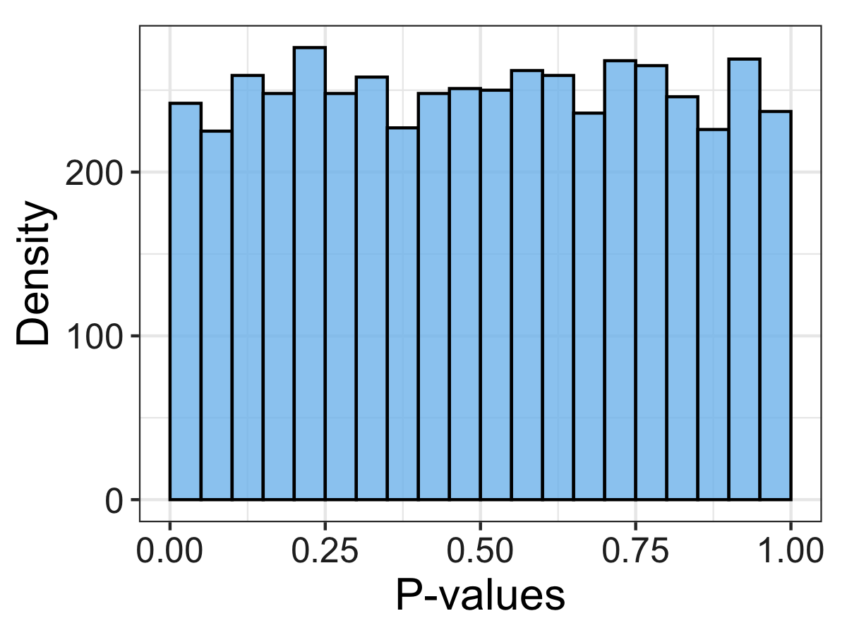
(b)

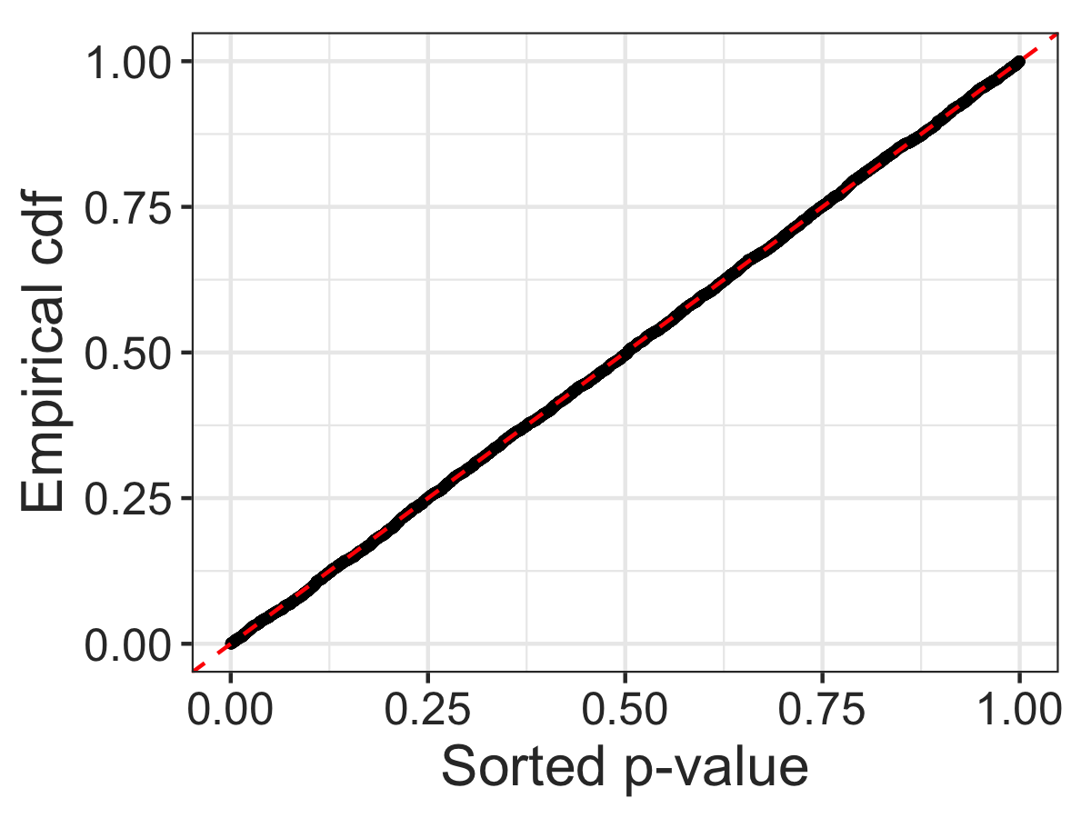
(c)

Figure 5: Distribution of null p-values from a two-sided $t$-test. Histograms of p-values are calculated by $p_{j}=2\bar{\Phi}(\sqrt{n}|\hat{\beta}_{j}|/\hat{\sigma}_{j})$. (a) $\hat{\sigma}_{j}$ is taken to be the standard error from R. (b) $\hat{\sigma}_{j}=\hat{\sigma}/\hat{\tau}_{j}$, where $\hat{\sigma}$ is estimated by ProbeFrontier and $\hat{\tau}_{j}$ is from (5.1) (c) Empirical cdf of the p-values in (b).

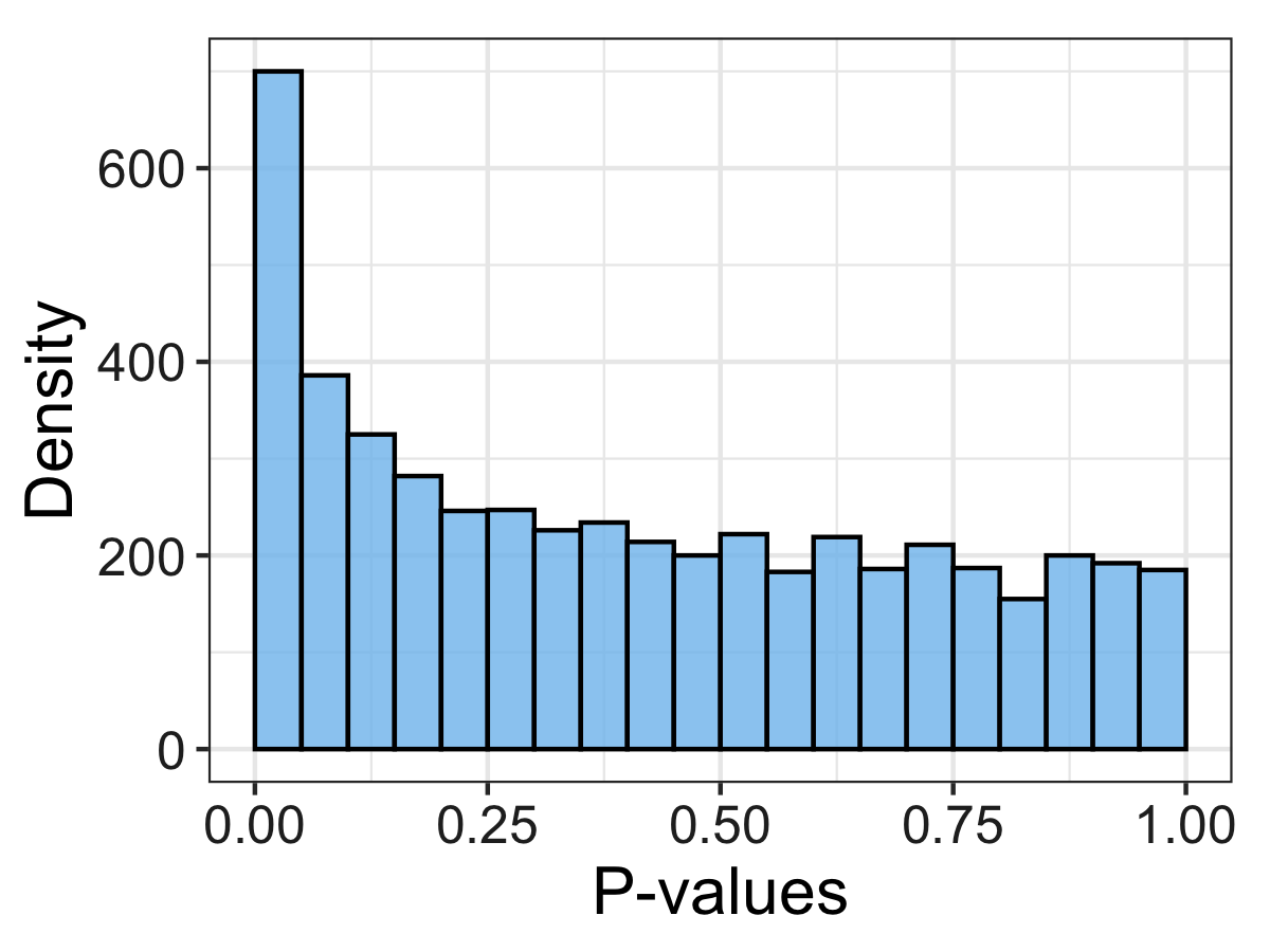
(a)

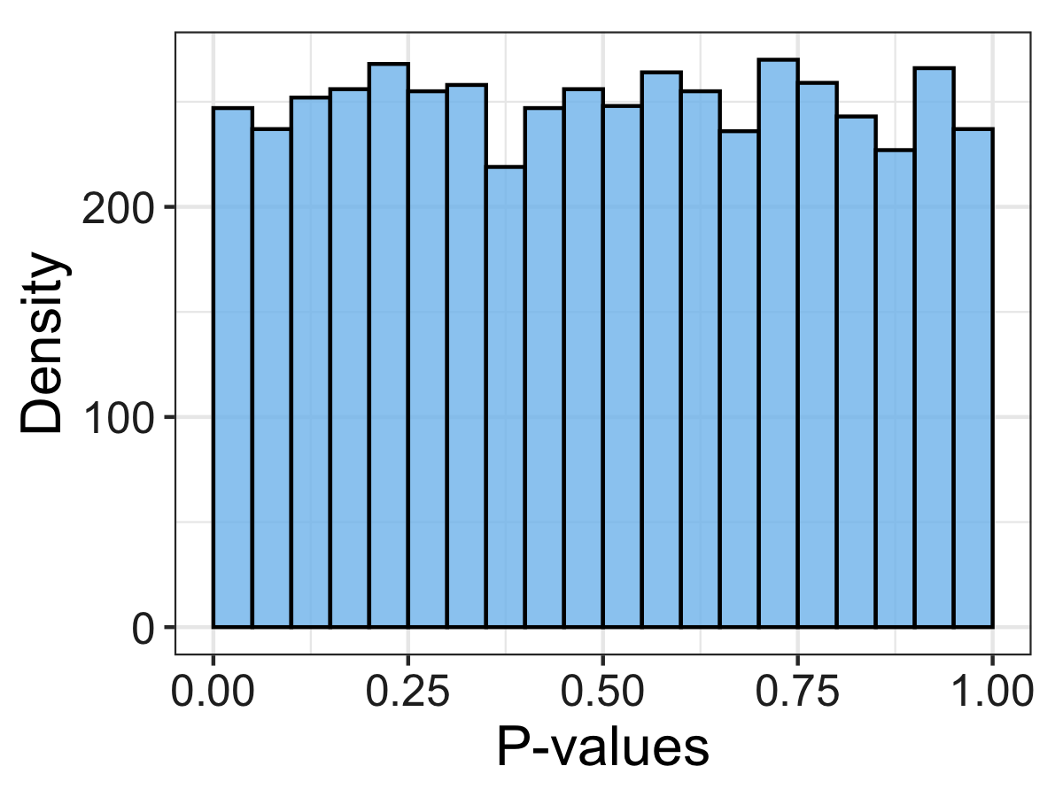
(b)

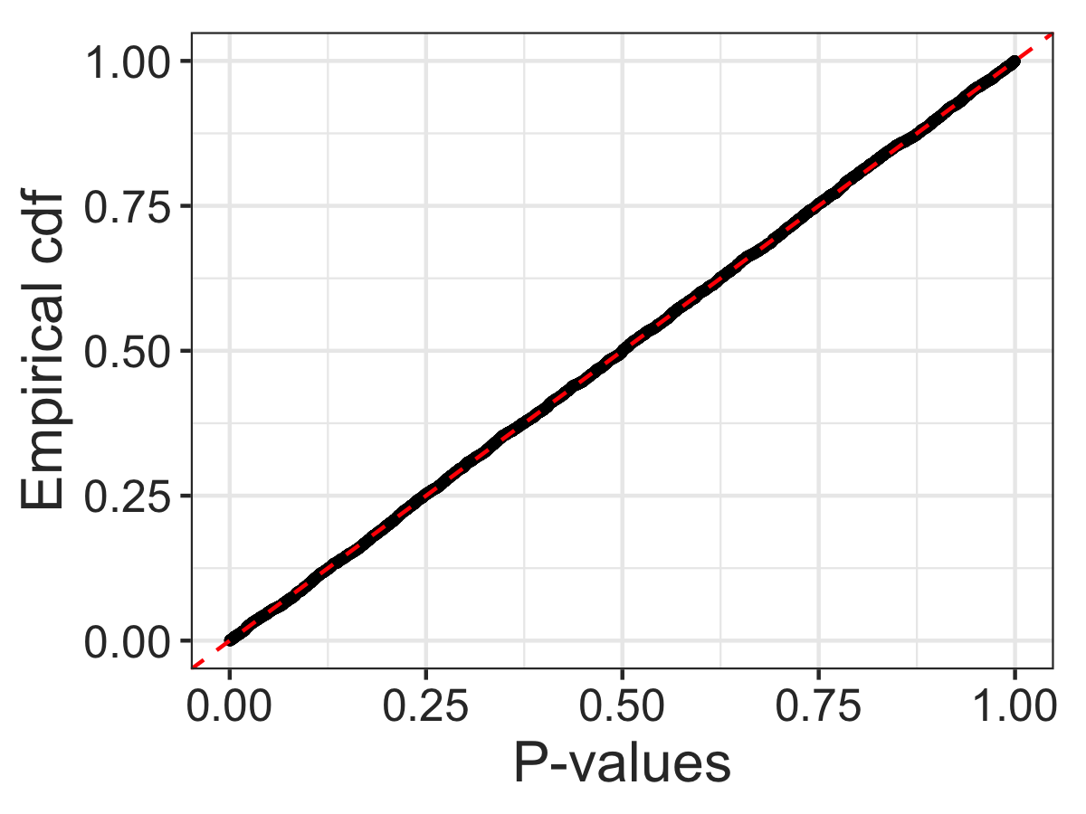
(c)

Figure 6: Distribution of null p-values calculated from the LRT (a) Histogram of p-values based on the chi-squared distribution (with 1 degree of freedom). (b) Histogram of p-values based on the re-scaled chi-squared distribution; the re-scaling factor is estimated by ProbeFrontier. (c) Empirical cdf of p-values from (b).

Table 7: Empirical performance of testing a null. Each cell reports the p-value probability and its standard error (in parentheses) estimated over $B=5,000$ repetitions. The p-values are calculated from a two sided $t$-test (as in Figure 5(c)) and the LRT (as in Figure 6(c)).

	$t$-test	LRT
$\mathbb{P}(\text{P-value}\leq 10\%)$	9.34% (0.41%)	9.68% (0.41%)
$\mathbb{P}(\text{P-value}\leq 5\%)$	4.84% (0.30%)	4.94% (0.30%)
$\mathbb{P}(\text{P-value}\leq 1\%)$	0.96% (0.14%)	0.94% (0.14%)
$\mathbb{P}(\text{P-value}\leq 0.1\%)$	0.08% (0.04%)	0.08% (0.04%)

6.3 Coverage proportion

We proceed to check the accuracy of the confidence intervals described by (5.3). We consider a single coordinate $\beta_{j}$ (we chose $\beta_{j}\neq 0$) and report the proportion of times (5.3) covers $\beta_{j}$ across the $B$ repetitions (Table 8). At each level, the empirical coverage proportion agrees with the desired target level, validating the marginal distribution (3.5) in non-Gaussian settings. To investigate the efficacy of (3.5) further, we calculate the standardized versions of the MLE given by

$$\hat{T}_{j}=\frac{\sqrt{n}(\hat{\beta}_{j}-\hat{\alpha}\beta_{j})}{\hat{\sigma}/\hat{\tau}_{j}}$$ (6.1)

for each run of the experiment; recall that the estimates $\hat{\alpha},\hat{\sigma},\hat{\tau}_{j}$ arise from the ProbeFrontier method and (5.1). Figure 7 displays a qqplot of the empirical quantiles of $\hat{T}_{j}$ versus the standard normal quantiles, and once again, we observe a remarkable agreement.

Table 8: Coverage proportion of a single variable. Each cell reports the proportion of times $\beta_{j}$ falls within (5.3), calculated over $B=5,000$ repetitions; the standard errors are provided as well. The unknown signal strength $\gamma^{2}$ is estimated by ProbeFrontier.

Nominal coverage
$100(1-\alpha)$	99	98	95	90	80
Empirical coverage	99.04	97.98	94.98	89.9	80.88
Standard error	0.2	0.2	0.3	0.4	0.6

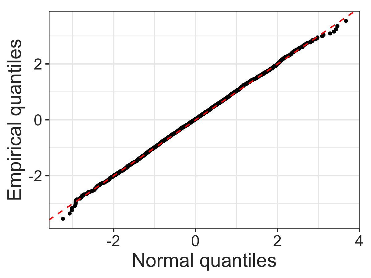
Figure 7: Quantiles of the empirical distribution of the MLE coordinate from Table 8, standardized as in (6.1), versus standard normal quantiles.

Finally, we turn to study the performance of Theorem 3.2. In each experiment, we compute the proportion of variables covered by the corresponding intervals in (5.3) and report the mean (Table 9) across the $5000$ replicates. Once again, the average coverages remained close to the desired thresholds for all the levels considered, demonstrating the applicability of the bulk result (3.10) beyond the setting of Gaussian covariates.

Table 9: Proportion of variables inside the confidence intervals (5.3). Each cell reports the average coverage estimated over $B=5,000$ repetitions. The standard errors are shown as well.

Nominal coverage
$100(1-\alpha)$	98	95	90	80
Empirical coverage	98.03	95.14	90.1	80.2
Standard error	0.01	0.01	0.02	0.02

7 Models with an intercept

In this section, we study the asymptotic distribution of a logistic MLE when the model contains an intercept, i.e. the likelihood of $y_{i}$ conditional on the covariates $\boldsymbol{x}_{i}$ is given by

$$\operatorname{\mathbb{P}}(y_{i}=1\,|\,\boldsymbol{x}_{i})=1/(1+\exp(-y_{i}(\beta_{0}+\boldsymbol{x}_{i}^{\top}\boldsymbol{\beta}))).$$ (7.1)

Suppose the intercept $\beta_{0}=o(1)$, then all the earlier theorems about the distribution of $\hat{\beta}_{j}$ and $\operatorname{LLR}_{j}$ apply as long as $j\geq 1$; the parameters in Theorem 3.1 and Theorem 4.1 are still solutions to (3.4). On the other hand, we conjecture that when $\beta_{0}$ is not asymptotically negligible, the MLE remains asymptotically Gaussian as in Theorem 3.1, but the parameters $\alpha_{\star}$ $\sigma_{\star}$ and $\lambda_{\star}$ now depend on $\beta_{0}$ as well as $\kappa$ and $\gamma$. (The phase transition curve in [9, Theorem 2.1] also depends on both $\gamma$ and $\beta_{0}$.) We conduct simulation studies to verify our conjecture (Section 7.1.1) and discuss how to estimate these parameters when the intercept is unknown (Section 7.2).

7.1 Asymptotic distribution of the MLE

Before we describe our conjecture when $\beta_{0}\neq o(1)$, we note that Proposition 2.1 and Lemma 2.1 applied to $\{\hat{\beta}_{j}\}_{j\geq 1}$—all coordinates except the intercept term—still hold because the rotation invariance argument operates in the same way. Thus, to establish the asymptotic MLE distribution, we only need to study the limit of $\alpha(n)$ and $\sigma(n)$ defined in Eqn. (2.7). We conjecture that, as $n,p\to\infty$ while $p/n\to\kappa$, $\alpha(n)$ and $\sigma(n)$ approach limits that can be determined by solving a system of four equations.

Conjecture 7.1.

Consider the logistic regression model (7.1) and assume that $(\kappa,\gamma,\beta_{0})$ is such that the MLE exists asymptotically. Denote $\hat{\beta}_{0}$ to be the MLE of the intercept and define $\alpha(n)$, $\sigma(n)$ as in Eqn. (2.7). Then, as $n,p\to\infty$ and $p/n\to\kappa>0$,

$$\hat{\beta}_{0}\stackrel{{\scriptstyle P}}{{\longrightarrow}}b_{\star},\quad\alpha(n)\stackrel{{\scriptstyle P}}{{\longrightarrow}}\alpha_{\star},\quad\sigma(n)\stackrel{{\scriptstyle P}}{{\longrightarrow}}\sigma_{\star},$$ (7.2)

and Theorem 3.1 and Theorem 4.1 hold with the set of parameters in (7.2). In (7.2), $\alpha_{\star},\sigma_{\star},b_{\star}$ are such that together with another constant $\lambda_{\star}$, these solve a system of equations in four variables $(\alpha,\sigma,\lambda,b)$ given by

$$\begin{dcases}&\kappa^{2}\sigma^{2}=\mathbb{E}\left[\rho^{\prime}(-S_{1})\left(\lambda\rho^{\prime}(\mathsf{prox}_{\lambda\rho}(S_{2}))\right)^{2}+\rho^{\prime}(S_{1})\left(\lambda\rho^{\prime}(\mathsf{prox}_{\lambda\rho}(-S_{2}))\right)^{2}\right]\\ &1-\kappa=\mathbb{E}\left[\frac{\rho^{\prime}(-S_{1})}{1+\lambda\rho^{\prime\prime}(\mathsf{prox}_{\lambda\rho}(S_{2}))}+\frac{\rho^{\prime}(S_{1})}{1+\lambda\rho^{\prime\prime}(\mathsf{prox}_{\lambda\rho}(-S_{2}))}\right]\\ &0=\mathbb{E}\left[\rho^{\prime}(\mathsf{prox}_{\lambda\rho}(S_{2}))\rho^{\prime}(-S_{1})S_{1}-\rho^{\prime}(\mathsf{prox}_{\lambda\rho}(-S_{2}))\rho^{\prime}(S_{1})S_{1}\right]\\ &0=\mathbb{E}\left[-\rho^{\prime}(\mathsf{prox}_{\lambda\rho}(-S_{2}))\rho^{\prime}(S_{1})+\rho^{\prime}(\mathsf{prox}_{\lambda\rho}(S_{2}))\rho^{\prime}(-S_{1})\right].\end{dcases}$$ (7.3)

where $(Z_{1},Z_{2})\sim\mathcal{N}(0,\boldsymbol{I}_{2})$ and

$$S_{1}=\gamma Z_{1}+\beta_{0},\quad S_{2}=\alpha\gamma Z_{1}+\sigma\sqrt{\kappa}Z_{2}+b.$$ (7.4)

$S_{1}$ and $S_{2}$ defined in (7.4) are related to $Q_{1}$ and $Q_{2}$ in Eqn. (3.4) as $S_{1}=-Q_{1}+\beta_{0}$ and $S_{2}=Q_{2}+b$. Compared to Eqn. (3.4), Eqn. (7.3) has four equations, and the fourth equation characterizes the limit of the estimated intercept. When $\beta_{0}=0$, the set of equations (7.3) reduces to the system of equations (3.4).

In sum, Conjecture 7.1 states that the marginal distribution of a logistic MLE $\hat{\beta}_{j}$ is asymptotically Gaussian with mean $\alpha_{\star}\beta_{j}$ and variance $\sigma_{\star}^{2}/\tau_{j}^{2}$, where the parameters $\alpha_{\star}$ and $\sigma_{\star}$ are determined by Eqn. (7.3).

7.1.1 Finite sample accuracy

We study the accuracy of our conjecture through simulated examples, where we fix $\beta_{0}=1$, but otherwise use the same setting as in Section 3.3. First, we report the coverage probability of a single non-null variable on using the confidence interval from Eqn. (3.8) (Table 10). Although the confidence intervals slightly undercovers the true coefficient, they are reasonably accurate as the error is within 0.5%. We also report the coverage proportion of all of the variables (Table 11) which shows that the $(1-\alpha)$ confidence interval covers approximately $(1-\alpha)$ of all of the variables in a single-shot experiment. We report results for different covariance matrices in the supplementary material [46, Section D], and observe that the performance is consistent across different types of matrices. Finally, we compute the adjusted p-values for a likelihood ratio statistics and report the distributions of p-values (Table 12). The adjusted p-values achieve the desired type I error because the proportion of p-values below each level is as we expect.

Table 10: Coverage proportion of a single non-null variable when the logistic model includes an intercept $\beta_{0}=1$ and the covariance matrix is defined as $\Sigma_{i,j}=0.5^{|i-j|}$. Each cell reports the proportion of times $\beta_{j}$ falls within the adjusted $(1-\alpha)$ CI using theoretical (Column I) and estimated parameters (Column II). The proportions are calculated over $B=100,000$ repetitions in Column I and $B=10,000$ in Column II, and the standard errors are provided as well.

	I. Theoretical		II. Estimated
Nominal coverage	Empirical	Standard	Empirical	Standard
$100(1-\alpha)$	coverage	error	coverage	error
99	98.96	0.03	98.74	0.11
98	97.90	0.05	97.71	0.15
95	94.86	0.07	94.56	0.23
90	89.83	0.10	89.18	0.31
80	79.88	0.13	79.34	0.40

Table 11: Each cell reports the proportion of all the variables in each run that fall within the corresponding intervals from (3.8) when $\beta_{0}=1$ in the same experiment as for Table 10. The standard errors are provided as well.

	I. Theoretical		II. Estimated
Nominal coverage	Empirical	Standard	Empirical	Standard
$100(1-\alpha)$	coverage	error	coverage	error
99	98.897	0.002	98.79	0.11
98	97.858	0.003	97.73	0.11
95	94.811	0.005	94.64	0.12
90	89.790	0.008	89.55	0.12
80	79.808	0.010	79.49	0.12

Table 12: Empirical performance of the LRT using adjusted p-values when the model has an intercept $\beta_{0}=1$. Each cell reports the p-value probability for a random null coordinate estimated in $B=10,000$ repetitions and the standard errors are provided in parentheses. Column I uses theoretical parameters, column II uses estimated parameters and Column III uses classical theory without adjustment.

	I. Theoretical	II. Estimated	III. Classical
$\mathbb{P}(\text{P-value}\leq 10\%)$	9.98 (0.30)	10.04 (0.30)	18.93 (0.45)
$\mathbb{P}(\text{P-value}\leq 5\%)$	4.92 (0.21)	5.02 (0.22)	11.62 (0.41)
$\mathbb{P}(\text{P-value}\leq 1\%)$	0.90 (0.09)	0.99 (0.10)	3.78 (0.29)
$\mathbb{P}(\text{P-value}\leq 0.5\%)$	0.54 (0.07)	0.61 (0.08)	2.46 (0.25)

7.1.2 Effect of the intercept

We study the effect of $\beta_{0}$ on the parameters $\alpha_{\star}$ and $\sigma_{\star}$ by showing the theoretical predictions at $\gamma^{2}=5$ for different choices of $\beta_{0}$ (Table 13). We observe that all of the parameters increase as $\beta_{0}$ increases (Column I). We should thus not ignore the intercept when it is not trivially small. Because the intercept term is not Gaussian, a model with an explicit intercept term is not equivalent to a model without an explicit intercept term and a matching overall signal strength. As a demonstration, we compare the parameters obtained here with solutions to the system of three equations (3.4) when we merge the intercept with the other coefficients, i.e. setting $\gamma=\sqrt{5+\beta_{0}^{2}}$. This approximation is accurate unless $\beta_{0}$ is large, for example, $\beta_{0}=2$ as in Table 13, row 4.

Table 13: The theoretical parameters for different $\beta_{0}$ when $\gamma^{2}=5$. Column I shows the solutions to the system of four equations (7.3) while Column II shows the solution to the system of three equations (3.4) assuming $\beta_{0}=0$ and $\gamma=\sqrt{5+\beta_{0}^{2}}$.

	I. Theoretical parameters				II. Merging intercept
$\beta_{0}$	$\alpha_{\star}$	$\sigma_{\star}$	$\lambda_{\star}$	$b_{\star}$	$\sqrt{5+\beta_{0}^{2}}$	$\alpha_{\star}$	$\sigma_{\star}$	$\lambda_{\star}$
0	1.50	4.75	3.03	0	2.24	1.50	4.75	3.03
0.5	1.51	4.84	3.13	0.76	2.29	1.51	4.84	3.12
1	1.56	5.16	3.45	1.559	2.45	1.55	5.13	3.42
2	1.83	7.01	5.47	3.68	3.00	1.75	6.45	4.83
2.5	2.31	10.00	8.96	5.80	3.35	1.95	7.73	6.26

7.2 Estimating model parameters

Conjecture 7.1 suggests that the MLE distribution for logistic models with intercepts is determined by $\kappa$, $\gamma$ and $\beta_{0}$. In this section, we introduce a procedure to estimate the unknown $\gamma$ and $\beta_{0}$ based on two observable quantities. First, the phase transition curve [9] determines a problem dimension $\kappa_{s}=h(\beta_{0},\gamma)$ such that if $\kappa>\kappa_{s}$, then the MLE does not exist asymptotically almost surely. We use the ProbeFrontier (see Section 5.1) method to estimate $\kappa_{s}$. In turn, the estimated $\hat{\kappa}_{s}$ provides the estimating equation

$$h(\beta_{0},\gamma)=\hat{\kappa}_{s}.$$ (7.5)

Second, the marginal probability $p$ of observing a positive outcome is determined by $\beta_{0}$ and $\gamma$ since

$$p=\operatorname{\mathbb{P}}(Y=1)=\mathbb{E}\left[1/{1+\exp(-\beta_{0}-\gamma Z)}\right],\quad Z\sim\mathcal{N}(0,1).$$

Here, we substitute a Gaussian variable for $X^{\top}\beta$, since $X^{\top}\beta\sim\mathcal{N}(0,\gamma^{2})$. We therefore use the observed proportion of positive outcomes $\hat{p}$ to get a second estimating equation

$$\mathbb{E}\left[1/{1+\exp(-\beta_{0}-\gamma Z)}\right]=\hat{p}.$$ (7.6)

Solving (7.5) and (7.6) gives $(\hat{\beta}_{0},\hat{\gamma})$, which is then plugged into (7.3) to compute $\hat{\alpha}$ and $\hat{\sigma}$. Eqn. (5.3) then provides adjusted $(1-\alpha)$ confidence interval for a single coefficient $\beta_{j}$.

Finally, we evaluate the empirical coverage of (5.3). As in Section 5, we compute the coverage proportion of a single non-null variable (Table 10) and across all of the variables (Table 11). We also study the performance of the LRT using estimated parameters (Table 12). Empirical coverage is accurate since it is within three standard deviations from the nominal value. The coverage across all of the variables is slightly smaller than nominal, but the relative error is within 1%. The adjusted p-values for the LRT also control the type I error. We can also see that the results obtained by using the estimated parameters compare favorably to those obtained using the theoretical parameters.

8 Is this all real?

We have seen that in logistic models with Gaussian covariates of moderately high dimensions, (a) the MLE overestimates the true effect magnitudes, (b) the classical Fisher information formula underestimates the true variability of the ML coefficients, and (c) classical ML based null p-values are far from uniform. We introduced a new maximum likelihood theory, which accurately amends all of these issues and demonstrated empirical accuracy on non-Gaussian light-tailed covariate distributions. We claim that the issues with ML theory apply to a broader class of covariate distributions; in fact, we expect to see similar qualitative phenomena in real datasets.

Consider the wine quality data [2], which contains 4898 white wine samples from northern Portugal. The dataset consists of 11 numerical variables from physico-chemical tests measuring various characteristics of the wine, such as density, pH and volatile acidity, while the response records a wine quality score that takes on values in $\{0,\ldots,10\}$. We define a binary response by thresholding the scores, so that a wine receives a label $y=0$, if the corresponding score is below $6$, and a label $y=1$, otherwise. We log-transform two of the explanatory variables as to make their distribution more symmetrical and concentrated. We also center the variables so that each has mean zero.

We explore the behavior of the classical logistic MLE for the variable “volatile acidity” ($\mathrm{va}$) at a grid of values of the problem dimension $\kappa\in K$. For each $\kappa\in K$, we construct $B=100$ subsamples containing $n=p/\kappa$ observations and calculate the MLE $\hat{\beta}_{\mathrm{va}}$ from each subsample. Figure 8 shows the boxplots of these estimated coefficients. Although the ground truth is unknown, the red dashed line plots the MLE $\hat{\beta}_{\mathrm{va}}=-6.18$ calculated over all 4898 observations so that it is an accurate estimate of the corresponding parameter. Noticeably, the ML coefficients move further from the red line, as the dimensionality factor increases, exhibiting a strong bias. For instance, when $\kappa$ is in $\{0.10,0.18,0.26\}$, the median MLE is repectively equal to $\{-7.48,-9.43,-10.58\}$; that is, $\{1.21,1.53,1.71\}$ times the value of the MLE (in magnitude) from the full data. These observations support our hypothesis that, irrespective of the covariate distribution, the MLE increasingly overestimates effect magnitudes in high dimensions.

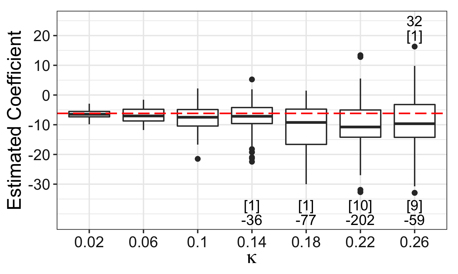
Figure 8: Estimated coefficient $\hat{\beta}_{\mathrm{va}}$ of the variable “volatile acidity”, obtained from $B=100$ sub-samples of size $p/\kappa$. The red dashed line shows the MLE using all the observations. The numbers of outliers outside of range are those between squared brackets. The minimum/maximum value of these outliers is given by the accompanying integer.

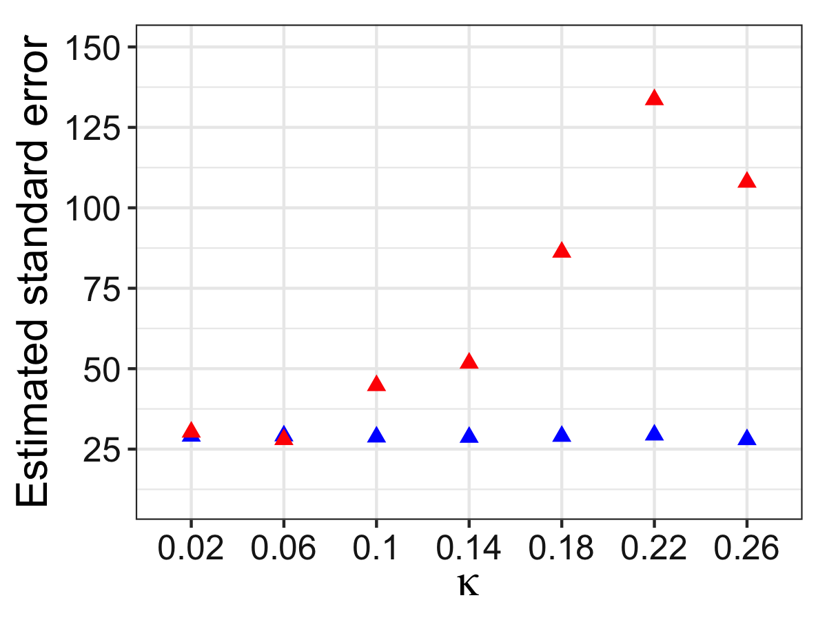
(a)

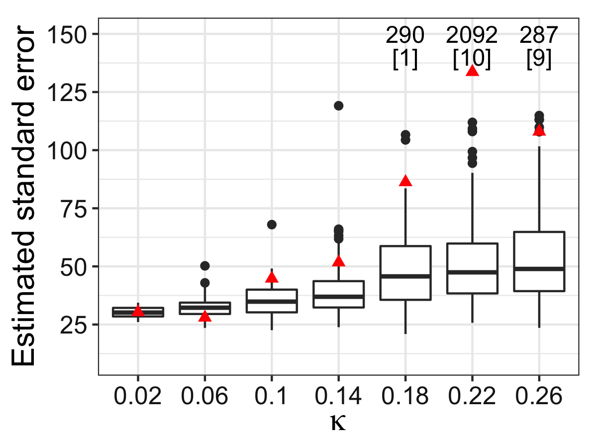
(b)

Figure 9: Comparison of standard errors adjusted for the sample size. Throughout, the red triangles represent an estimate of the standard deviation (sd) of the MLE for “volatile acidity”, obtained by creating folds of sample size $p/\kappa$ and computing the sd across these folds. To evidence the bias, the estimated standard deviations (blue) are multiplied by the root sample size (see text). (a) Estimated sd given by the inverse Fisher information (adjusted for sample size) averaged over $B=100$ subsamples for each value of $\kappa$. (b) Standard error (adjusted for sample size) from R calculated in each subsample. (The meaning of the numbers in between square brackets and their accompanying integer is as in Figure 8.)

Next, Figure 9 compares the standard deviation (sd) in high dimensions with the corresponding prediction from the classical Fisher information formula. Theorem 3.1 states that when $n$ and $p$ are both large and the covariates follow a multivariate Gaussian distribution, $\hat{\beta}_{j}$ approximately obeys

$$\hat{\beta}_{j}=\alpha_{\star}(\kappa)\beta_{j}+\sigma_{\star}(\kappa)Z/\sqrt{n},$$ (8.1)

where $Z\sim\mathcal{N}(0,1)$. If we reduce $n$ by a factor of 2, the standard deviation should increase by a factor of $\sigma_{\star}(2\kappa)/\sigma_{\star}(\kappa)\times\sqrt{2}$. Thus, in order to evidence the interesting contribution, namely, the factor of $\sigma_{\star}(2\kappa)/\sigma_{\star}(\kappa)$, we plot $\sqrt{n}\times\mathrm{sd}(\hat{\beta}_{\mathrm{va}})$, where $n$ is the sample size used to calculate our estimate.

With the sample size adjustment, we see in Figure 9(a) that the variance of the ML coefficient is much higher than the corresponding classical value, and that the mismatch increases as the problem dimension increases. Thus, we see once more a “variance inflation” phenomenon similar to that observed for Gaussian covariates (see also, [14, 6]). To be complete, we here approximate/estimate the (inverse) Fisher information as follows: for each $\kappa\in K$, we form $\hat{\mathcal{I}}(\boldsymbol{\beta})=\frac{1}{B}\sum_{j=1}^{B}\boldsymbol{X}_{j}^{\prime}\boldsymbol{D}_{\boldsymbol{\beta}}\boldsymbol{X}_{j}$, where $\boldsymbol{X}_{j}$ is the covariate matrix from the $j$-th subsample, and for $\boldsymbol{\beta}$, we plug in the MLE from the full data.

Standard errors obtained from software packages are different from those shown in Figure 9(a), since these typically use the maximum likelihood estimate $\hat{\boldsymbol{\beta}}$ from the data set at hand as a plug-in for $\boldsymbol{\beta}$, and in addition, do not take expectation over the randomness of the covariates. However, since these estimates are widely used in practice, it is of interest to contrast them with the true standard deviations. Figure 9(b) presents a boxplot of standard errors of $\hat{\beta}_{\mathrm{va}}$ (adjusted for sample size) as obtained from R. Observe that for large values of $\kappa$, these also severely underestimate the true variability.

9 Discussion

This paper establishes a maximum likelihood theory for high-dimensional logistic models with arbitrarily correlated Gaussian covariates. In particular, we establish a stochastic representation for the MLE that holds for finite sample sizes. This in turn yields a precise characterization of the finite-dimensional marginals of the MLE, as well as the average behavior of its coordinates. Our theory relies on the unknown signal strength parameter $\gamma$, which can be accurately estimated by the ProbeFrontier method. This provides a valid procedure for constructing p-values and confidence intervals for any finite collection of coordinates. Furthermore, we observe that our procedure produces reliable results for moderate sample sizes, even in the absence of Gaussianity—in particular, when the covariates are light-tailed.

We conclude with a few directions of future research—it would be of interest to understand (a) the class of covariate distributions for which our theory, or a simple modification thereof, continues to apply, (b) the class of generalized linear models for which analogous results hold, and finally, (c) the robustness of our proposed procedure to model misspecifications.

References

- [1] Anastasiou, A. and Reinert, G. (2020). Bounds for the asymptotic distribution of the likelihood ratio. Ann. Appl. Probab. 30 608–643.
- [2] Àngela, N. and Francisco, M. and Antoni, E. (2015). Modeling wine preferences from physicochemical properties using fuzzy techniques. Proceedings of the 5th International Conference on Simulation and Modeling Methodologies, Technologies and Applications. SciTePress. 501–507.
- [3] Bayati, M. and Montanari A. (2011). The dynamics of message passing on dense graphs, with applications to compressed sensing. IEEE Trans. Inform. Theory 57 764–785.
- [4] Bühlmann, P. and van der Geer, S. (2011). Statistics for High-dimensional Data: Methods, Theory and Applications. Heidelberg; New York: Springer.
- [5] Bellec, P. C. and Zhang, C.-H. (2019). Second order Poincaré inequalities and de-biasing arbitrary convex regularizers when . arXiv preprint arXiv:1912.11943.
- [6] Donoho, D. and Montanari, A. (2016). High dimensional robust M-estimation: asymptotic variance via approximate message passing. Probab. Theory Related Fields 166 935–969.
- [7] Barbier, J. and Krzakala, F. and Macris, N. and Miolane, L. and Zdeborová, L. (2019). Optimal errors and phase transitions in high-dimensional generalized linear models. Proc. Natl. Acad. Sci. USA. 116 5451–5460.
- [8] Bayati, M. and Montanari, A. (2011). The Lasso risk for Gaussian matrices. IEEE Trans. Inform. Theory 58 1997–2017.
- [9] Candès, E. J. and Sur, P. (2020). The phase transition for the existence of the maximum likelihood estimate in high-dimensional logistic regression. Ann. Statist. 48 27–42.
- [10] Celentano, M. and Montanari, A. and Wei, Y. (2020). The Lasso with general Gaussian designs with applications to hypothesis testing. arXiv preprint arXiv:2007.13716.
- [11] Chatterjee, S. (2009). Fluctuations of eigenvalues and second order Poincaré inequalities. Probab. Theory Related Fields 143 1–40.
- [12] Tony Cai, T. and Guo, Z. (2020). Semisupervised inference for explained variance in high-dimensional linear regression and its applications. J. R. Stat. Soc. Ser. B. Stat. Methodol. 82 391–419.
- [13] Donoho, D. and Maleki, A. and Montanari, A.(2009). Message-passing algorithms for compressed sensing. Proc. Natl. Acad. Sci. USA 106 18914–18919.
- [14] El Karoui, N. and Bean, D. and Bickel, P. J. and Lim, C. and Yu, B. (2013). On robust regression with high-dimensional predictors. Proc. Natl. Acad. Sci. USA 110 14557–14562.
- [15] El Karoui, N. (2018). On the impact of predictor geometry on the performance on high-dimensional ridge-regularized generalized robust regression estimators. Probab. Theory Related Fields 170 95–175.
- [16] Fan, Y. and Demirkaya, E. and Lv, J. (2019). Nonuniformity of P-values can occur early in diverging dimensions. J. Mach. Learn. Res. 20 1–33.
- [17] van der Geer, S. and Bühlmann, P. and Ritov, Y. and Dezeure, R. (2014). On asymptotically optimal confidence regions and tests for high-dimensional models. Ann. Statist. 42 1166–1202.
- [18] Gordon, Y (1988). On Milman’s inequality and random subspaces which escape through a mesh in . Geometric Aspects of Functional Analysis. Lecture Notes in Mathematics. 1317. Springer, Berlin, Heidelberg.
- [19] He, X. and Shao, Q.-M. (2020). On parameters of increasing dimensions. J. Multivariate Anal. 73 120–135.
- [20] Javanmard, A. and Montanari, A. (2013). State evolution for general approximate message passing algorithms, with applications to spatial coupling. Inf. Inference 2 115–144.
- [21] Javanmard, A. and Montanari, A. (2014). Confidence intervals and hypothesis testing for high-dimensional regression. J. Mach. Learn. Res. 15 2869–2909.
- [22] Janková, J. and van de Geer, S. (2021). De-biased sparse PCA: inference and testing for eigenstructure of large covariance matrices. IEEE Trans. Inform. Theory. 67 2507–2527.
- [23] Kimmel, G. and Shamir, R. (2005). A block-free hidden Markov model for genotypes and its application to disease association. J. Comput. Biol. 12 1243–1260.
- [24] Montanari, A. (2018). Mean field asymptotics in high-dimensional statistics: from exact results to efficient algorithms. Proceedings of the International Congress of Mathematicians Rio de Janeiro 2018. Singapore: SBM: World Scientific. 1 2973–2994.
- [25] Mézard, M. and Parisi, G. and Virasoro, M. (1986). Spin Glass Theory and Beyond: An Introduction to the Replica Method and Its Applications. Singapore; [Teaneck] New Jersey: World Scientific, c1987.
- [26] McCullagh, P. and Nelder, J.A. (1989). Generalized Linear Models, 2nd ed. London; New York: Chapman and Hall, 1989.
- [27] Ma, R. and Tony Cai, T and Li, H. (2021). Global and simultaneous hypothesis testing for high-dimensional logistic regression models. J. Amer. Statist. Assoc. 116 984–998.
- [28] Portnoy, S. (1984). Asymptotic behavior of M-estimators of regression parameters when is large. I. consistency. Ann. Statist. 12 1298–1309.
- [29] Portnoy, S. (1985). Asymptotic behavior of M-estimators of regression parameters when is large; II. normal approximation. Ann. Statist. 12 1403–1417.
- [30] Portnoy, S. (1988). Asymptotic behavior of likelihood methods for exponential families when the number of parameters tends to infinity. Ann. Statist. 16 356–366.
- [31] Rastas, P. and Koivisto, M. and Mannila, H. and Ukkonen, E. (2005). A hidden Markov technique for haplotype reconstruction. Algorithms in Bioinformatics. WABI 2005. Lecture Notes in Computer Science. 3692 Springer, Berlin, Heidelberg.
- [32] Rangan, S. (2011). Generalized approximate message passing for estimation with random linear mixing. 2011 IEEE International Symposium on Information Theory Proceedings.
- [33] Sabatti, C. and Candès, E. J. and Sesia, M. (2018). Gene hunting with hidden Markov model knockoffs. Biometrika 106 1–18.
- [34] Salehi, F. and Abbasi, E. and Hassibi, B. (2019). The impact of regularization on high-dimensional logistic regression. Proceedings of the 33rd International Conference on Neural Information Processing Systems.
- [35] Sesia, M. (2019). Using SNPknock with genetic data. https://msesia.github.io/snpknock/articles/genotypes.html, [online; accessed 30-October-2019].
- [36] Scheet, P. and Stephens, M. (2006). A fast and flexible statistical model for large-scale population genotype data: applications to inferring missing genotypes and haplotypic phase. Am. J. Hum. Genet. 78 629–644.
- [37] Sur, P. and Chen, Y. and Candès, E. J. (2019). The likelihood ratio test in high-dimensional logistic regression is asymptotically a rescaled chi-square. Probab. Theory Related Fields 175 487–558.
- [38] Sur, P. and Candès, E. J. (2019). A modern maximum-likelihood theory for high-dimensional logistic regression. Proc. Natl. Acad. Sci. USA 116 14516–14525.
- [39] Sur, P. (2019). A modern maximum-likelihood theory for high-dimensional logistic regression. Ph.D. thesis, Stanford University, purl.stanford.edu/jw604jq1260.
- [40] Thrampoulidis, C. and Oymak, S. and Hassibi, B. (2015). Regularized linear regression: a precise analysis of the estimation error. Proc. Mach. Learn. Res. 40 1683–1709.
- [41] Thrampoulidis, C. and Abbasi, E. and Hassibi, B. (2018). Precise error analysis of regularized M-estimators in high dimensions. IEEE Trans. Inform. Theory 64 5592–5628.
- [42] van der Vaart, A. W. (1998). Asymptotic Statistics. Cambridge, UK; New York, NY, USA: Cambridge University Press.
- [43] Wainwright, M. J. (2019). High-Dimensional Statistics: A Non-Asymptotic Viewpoint. Cambridge; New York, NY: Cambridge University Press.
- [44] Wilks, S. S. (1938). The large-sample distribution of the likelihood ratio for testing composite hypotheses. Ann. Statist. 9 60–62.
- [45] Zhang, C.-H. and Zhang, S.S. (2014). Confidence intervals for low dimensional parameters in high-dimensional linear models. J. R. Stat. Soc. Ser. B. Stat. Methodol. 76 217–242.
- [46] Zhao, Q., Sur, P. and Candès, E. J. (2021). Supplement to “The asymptotic distribution of the MLE in high-dimensional logistic models: arbitrary covariance.” DOI: 10.1214/[provided by typesetter].
- [47] Zhao, Q. (2020). Glmhd: statistical inference in high-dimensional binary regression, https://github.com/zq00/glmhd. R package version 0.0.0.9000.