LHC signals of triplet scalars as dark matter portal: cut-based approach and improvement with gradient boosting and neural networks

Abstract

We consider a scenario where an SU(2) triplet scalar acts as the portal for a scalar dark matter particle. We identify regions of the parameter space, where such a triplet coexists with the usual Higgs doublet consistently with all theoretical as well as neutrino, accelerator and dark matter constraints, and the triplet-dominated neutral state has substantial invisible branching fraction. LHC signals are investigated for such regions, in the final state same-sign dilepton + $\geq$ 2 jets + $\not E_{T}$. While straightforward detectability at the high-luminosity run is predicted for some benchmark points in a cut-based analysis, there are other benchmarks where one has to resort to gradient boosting/neural network techniques in order to achieve appreciable signal significance.

1 Introduction

The recent data on direct search for dark matter (DM), especially those from the Xenon1T observation Aprile:2018dbl , rather strongly constrain scenarios where the 125 GeV Higgs acts as dark matter portal. The coupling of, say, a scalar SU(2) singlet DM to the Higgs boson of the standard model (SM) is restricted by such constraints to be $\raisebox{-3.69899pt}{~{}\shortstack{$<$ \\ [-0.07cm] $\sim$}}~{}10^{-3}$. Ensuring the DM annihilation rate required for consistency with the observed relic density becomes a big challenge in such a case.

The restriction is considerably relaxed for an extended electroweak symmetry breaking sector. For example, in two-Higgs doublet models (2HDM), one can have regions in the parameter space where the DM candidate has rather feeble interaction with $h$, the SM-like scalar, but sufficient coupling with the heavier neutral scalar $H$ so as to be consistent with both direct search results and the relic density Drozd:2014yla . This can happen due to the large mass of a mediating $H$ suppressing the elastic scattering rates; it is also possible to have cancellation between the $h$ and $H$-mediated scattering amplitudes. The allowed regions in 2HDM satisfying such requirements and the corresponding signals at the Large Hadron Collider (LHC) have been studied in detail Dey:2019lyr .

Here we present the results of a similar investigation in the context of scalar triplet extension of the SM Magg:1980ut ; Schechter:1980gr ; Lazarides:1980nt ; Mohapatra:1980yp ; Cheng:1980qt ; Bilenky:1980cx ; Kobzarev:1980nk ; Gunion:1989ci ; Mukhopadhyaya:1990up ; Mohapatra:1991ng ; Ma:1998dx ; Chaudhuri:2013xoa ; Chaudhuri:2016rwo , together with a scalar DM candidate $\chi$ Krolikowski:2012jd . A $Y=2$ scalar triplet added to the SM doublet, with the triplet vacuum expectation value (VEV) limited to $\raisebox{-3.69899pt}{~{}\shortstack{$<$ \\ [-0.07cm] $\sim$}}~{}4.8$ GeV by the $\rho$-parameter Primulando:2019evb , can generate Majorana masses for neutrinos via the Type-II Seesaw mechanism. It also has a rich collider phenomenology Godbole:1994np ; Cheung:1994rp ; Ghosh:1996jg ; Perez:2008ha ; Du:2018eaw ; Ghosh:2018jpa , largely due to the presence of a doubly charged scalar that decays either to same-sign dileptons or same-sign $W$ pairs.

If the DM particle $\chi$, odd under a $Z_{2}$ symmetry, couples to such a triplet $\Delta$, the strength of the interaction is not subject to severe constraints. This is because the triplet cannot mediate the elastic scattering of $\chi$ against the quarks in a terrestrial detector, because of electroweak gauge invariance. On the other hand, the SM-like scalar doublet must again have suppressed interaction with $\chi$. The requisite DM annihilation rate in such a case can be ensured by an appropriate quartic interaction $\Delta^{\dagger}\Delta\chi^{2}$, on which no severe constraint exists. We have indeed found a substantial region in the parameter space, satisfying all constraints from direct search, relic density, neutrino masses and mixing, and of course collider searches for triplet scalars. We thereafter look for the LHC signals of such a scenario serving as DM portal, one of whose consequences is an invisible branching ratio for $H$, the physical state dominated by the neutral CP-even member of $\Delta$. This can be utilised in Drell-Yan (DY) processes involving the doubly charged scalar. The most profitable DY channel is found to be $pp\rightarrow H^{\pm\pm}H^{\mp}$, where $H^{\pm\pm},H^{\mp}$ are once more the doubly- and singly-charged mass eigenstate dominanted by components of the triplet. The $H^{\mp}$ in such a situation decays into $HW^{\mp}$; we latch on to the invisible decay of the $H$ into a DM pair, while the $W$ is identified in its hadronic decay channels.

The $\Delta L=2$ lepton Yukawa interactions of $\Delta$ generate neutrino masses. This puts constraints on the products of the triplet VEV multiplied by the Yukawa couplings strengths. When the VEV is small, relative large $\Delta L=2$ interactions make same-sign dileptons the dominant decay products of $H^{\pm\pm}$. In the other situation, namely, one where the triplet VEV is close to its experimental limit, this VEV drives the decay to $W^{\pm}W^{\pm}$ to be the principal mode. We find that the first scenario has especially clean signals, with large missing-$E_{T}$ ($\not{E_{T}}$) from invisible $H$-decay accompanied by a sharp dilepton mass peak. The event rate in vector boson fusion (VBF) channel is also estimated but found to be inadequate for detection of the signal. Lastly, we follow up of the cut-based analysis with a multivariate analysis based on gradient boosting, and also using the artificial neural network (ANN) technique.

The plan of this work is as follows. In Section 2, we present a brief outline of the model. In Section 3, we discuss all the relevant constraints on our model including those from Higgs sector, dark matter sector, electroweak presicion tests, neutrino data and theretical constraints. In Section 4, we choose appropriate final states and discuss interesting benchmark points for collider studies involving the model. In Section 5, we present the cut-based collider analysis for selected final states. In Section 6, we explore the scope for improvements using sophisticated neural network and gradient boosting analysis. We summarize our key findings of this work and conclude in Section 7.

2 A model with a triplet scalar and a scalar dark matter

We concentrate on an extension of a Type-II Seesaw scenario containing a $Y$ = 2 scalar triplet $\Delta$ along with a singlet scalar dark matter candidate $\chi$. $\chi$ interacts with $\Delta$ and the SM-like higgs doublet $\Phi$ via terms in the scalar potential. The Lagrangian of the full scenario is

$${\cal L}={\cal L}_{SM}+{\cal L}_{Type-IISeesaw}+{\cal L}_{DM}+{\cal L}_{Int}$$ (1)

where

$${\cal L}_{DM}+{\cal L}_{Int}=\frac{1}{2}\partial^{\mu}\chi\partial_{\mu}\chi-\frac{1}{2}M_{\chi}^{2}\chi^{2}+\lambda_{S}\chi^{4}+\lambda_{D}\chi^{2}\Phi^{\dagger}\Phi+\lambda_{T}\chi^{2}Tr(\Delta^{\dagger}\Delta)$$ (2)

$\chi$, an $SU(2)_{L}\times U(1)_{Y}$ singlet, does not have any vacuum expectation value (VEV). An additional $Z_{2}$ symmetry ensures this, under which $\chi$ is assumed to be odd but $\Phi$ and $\Delta$ are even. The $Z_{2}$ prevents $\chi$ from mixing with $\Phi$ and $\Delta$. Thus the phenomenological constraints on all particles/interactions except those involving $\chi$ are similar to those applicable on a Type-II Seesaw model.

The scalar potential of Type-II Seesaw model:

The most general Higgs potential involving $\chi$, $\phi$ and $\Delta$ can be written as

$$\mathcal{V}(\Phi,\Delta,\chi) = a\Phi^{\dagger}\Phi+\frac{b}{2}Tr(\Delta^{\dagger}\Delta)-\frac{1}{2}M_{\chi}^{2}\chi^{2}+c(\Phi^{\dagger}\Phi)^{2}+\frac{d}{4}\left(Tr(\Delta^{\dagger}\Delta)\right)^{2}$$ (3)

$$+ \frac{e-h}{2}\Phi^{\dagger}\Phi Tr(\Delta^{\dagger}\Delta)+\frac{f}{4}Tr(\Delta^{\dagger}\Delta^{\dagger})Tr(\Delta\Delta)+h\Phi^{\dagger}\Delta^{\dagger}\Delta\Phi+(t\Phi^{\dagger}\Delta\tilde{\Phi}+h.c)$$

$$+ \lambda_{S}\chi^{4}+\lambda_{D}\chi^{2}\Phi^{\dagger}\Phi+\lambda_{T}\chi^{2}Tr(\Delta^{\dagger}\Delta)\,.$$

where, $\tilde{\Phi}\equiv i\tau_{2}\Phi^{\ast}$. This scalar sector is expressed in terms of additional scalar triplet with usual scalar doublet

$$\Phi(1,2,+1)=\left(\begin{array}[]{c}\phi^{+}\\ \phi^{0}\end{array}\right)\quad\mbox{and}\quad\Delta(1,3,+2)=\left(\begin{array}[]{cc}\delta^{+}&\sqrt{2}\delta^{++}\\ \sqrt{2}\delta^{0}&-\delta^{+}\end{array}\right)\,.$$ (4)

The numbers in parentheses denotes their representation under SM Gauge group $SU(3)_{C}\times SU(2)_{L}\times U(1)_{Y}$.

The VEVs of the doublet and the triplet are given by

$$\langle\Phi_{0}\rangle=\left(\begin{array}[]{c}0\\ v_{D}\end{array}\right)\quad\mbox{and}\quad\langle\Delta_{0}\rangle=\left(\begin{array}[]{cc}0&0\\ 0&v_{T}\end{array}\right)\,.$$ (5)

We concentrate now on the part of (Equation 3) involving $\Phi$ and $\Delta$ alone. All the parameters we choose are real, excepting $t$ which can be complex in general. Thus we write $t=|t|e^{i\gamma^{{}^{\prime}}}$ and $v_{T}=\omega e^{i\gamma}$ with $\omega\equiv|v_{T}|$. The orders of magnitude for the other parameters in the potential are indicated as

$$a,\>b\sim v^{2}\>;\quad c,\>d,\>e,\>f,\>h\sim 1\>;\quad|t|\ll v\,.$$ (6)

where $v=\sqrt{{v_{D}}^{2}+2{v_{T}}^{2}}$. The minimum of the potential expressed in terms as of the VEVs, is given by  Grimus:1999fz

$$V(\langle\phi\rangle_{0},\langle\Delta\rangle_{0}) = \frac{1}{2}a{v_{D}}^{2}+\frac{1}{2}b\omega^{2}+\frac{1}{4}c{v_{D}}^{4}+\frac{1}{4}d\omega^{4}$$

$$+ \frac{1}{4}(e-h){v_{D}}^{2}\omega^{2}+{v_{D}}^{2}\omega|t|\cos(\gamma^{{}^{\prime}}+\gamma)\,.$$

The minimization condition in terms of $(v_{D},\omega,\cos(\gamma^{{}^{\prime}}+\gamma))$ yield $\gamma^{{}^{\prime}}+\gamma=\pi$ or

$$v_{T}=-\omega e^{-i\gamma^{{}^{\prime}}}\quad\mbox{and}\quad v_{T}t=-\omega|t|\,.$$ (8)

and

$$a+c{v_{D}}^{2}+\frac{e-h}{2}\omega^{2}-2|t|\omega = 0\,,$$ (9)

$$b+d\omega^{2}+\frac{e-h}{2}{v_{D}}^{2}-\frac{|t|}{\omega}{v_{D}}^{2} = 0\,.$$ (10)

with fields shifted with respect to the VEV’s, one can write

$$\Phi=\left(\begin{array}[]{c}\phi^{+}\\ \frac{v_{D}+\phi_{r}+i\phi_{i}}{\sqrt{2}}\end{array}\right)\quad\mbox{and}\quad\Delta=\left(\begin{array}[]{cc}\delta^{+}&\sqrt{2}\delta^{++}\\ v_{T}+\delta+i\eta&-\delta^{+}\end{array}\right)\,.$$ (11)

After Spontaneous Symmetry Breaking(SSB) three Goldstone bosons are eaten up by the $W$ and the $Z$ bosons. Thus after diagonalizing the mass matrices, one is left with a doubly charge scalar $H^{\pm\pm}\equiv\delta^{\pm\pm}$, a singly-charged scalar $H^{\pm}$ and two neutral scalars $h$ and $H$, along with a neutral pseudoscalar $A$. The corresponding mass eigenvalues are

$$m^{2}_{h} \simeq 2c{v^{2}_{D}}+\frac{(e-h-2q)^{2}}{2c-q}\omega^{2}\,,$$ (12)

$$m^{2}_{H} \simeq q{v^{2}_{D}}-\left[\frac{(e-h-2q)^{2}}{2c-q}-2d\right]\omega^{2}\,,$$ (13)

$$m^{2}_{A} = q({v^{2}_{D}}+4\omega^{2})\,,$$ (14)

$$m^{2}_{H^{\pm\pm}} = (h+q){v^{2}_{D}}+2f\omega^{2}\,,$$ (15)

$$m^{2}_{H^{\pm}} = (q+\frac{h}{2})({v^{2}_{D}}+2\omega^{2})\,$$ (16)

The diagonalization process also yields

$$\tan\alpha = \frac{\sqrt{(q-2c)^{2}{v_{D}}^{2}+(2dq-4cd+(h-e+2q)^{2})w^{2}}}{(h-e+2q)\omega}\,,$$ (17)

$$\tan\beta = \frac{2\omega}{v_{D}}\,,$$ (18)

$$\tan\beta^{{}^{\prime}} = \frac{\sqrt{2}\omega}{v_{D}}\,$$ (19)

where $\alpha$ is the mixing angle between the CP-even parts of $\Phi$ and $\Delta$, $\beta$ is the mixing angle in charge Higgs sector with the mixing angle $\beta^{{}^{\prime}}$ in the CP-odd Higgs sector. We can notice that only the CP-even scalars $h$ and $H$ can act as portal for dark matter where CP is conserved.

Gauge interactions:

The Gauge interaction terms are as usual as SM with additional term added for the triplet part

$${\cal L}_{gauge}=(D_{\mu}\Phi)^{\dagger}D^{\mu}\Phi+\frac{1}{2}Tr((D_{\mu}\Delta)^{\dagger}(D^{\mu}\Delta))$$ (20)

Where $D_{\mu}\Phi=\partial_{\mu}\Phi-\frac{i}{2}gW_{\mu}^{a}\tau^{a}\Phi-\frac{i}{2}g^{\prime}B_{\mu}\Phi$ and $D_{\mu}\Delta=\partial_{\mu}\Delta-\frac{i}{2}g[W_{\mu}^{a}\tau^{a},\Delta]-ig^{\prime}B_{\mu}\Delta$ and $\tau^{a}$ are the SU(2) generators.

The gauge interactions will turn out be useful in our scenario where $\lambda_{D}\ll\lambda_{T}$ and thus the triplet scalar serves effectively as dark matter portal. As we shall see, we need to utilize the Drell-Yan production of triplet dominated states, driven by gauge couplings, for signals identifying the DM particle $\chi$.

Yukawa interactions:

The triplet within this model have potential to induce Majorana neutrino masses via interactions with the left-handed lepton doublet $L\equiv(\nu,l)^{T}$  Perez:2008zc ; Primulando:2019evb . The Yukawa terms with $(\Delta L=2)$ can be written as

$${{\cal L}^{new}_{Y}}=\sqrt{2}f_{ab}{L_{a}}^{T}Ci\sigma^{2}\Delta L_{b}+h.c.$$ (21)

Where $C$ is the charge conjugation matrix and $a,b$ run over all three flavour indices. The neutrino masses are mostly dependent on the triplet VEV $w$ and can be expressed as

$$M_{\nu}=2f\omega$$ (22)

As $f_{ab}$ is symmetric under $a\leftrightarrow b$, $M_{\nu}$ turns out to be a symmetric matrix. We can get the masses of the neutrinos after the diagonalization of $M_{\nu}$ with the help of the Pontecorvo-Maki-Nakagawa-Sakata (PMNS) matrix.

3 Constraints and allowed regions of the parameter space

So long as there is small mixing between the dark matter particle $\chi$ and the scalar triplet and doublet, which is ensured by the smallness of the triplet VEV as compared to that of the doublet, the main constraints on the scalar sector remain similar as for the Type-II Seesaw model, as discussed in  Primulando:2019evb . We summarize them below, and turn to the additional constraints on the dark matter sector.

It is useful to constrain the model parameters in terms of physical masses and mixing angles. Thus we express the parameters in the potential as

$$d = \frac{1}{2\omega^{2}}\left[\frac{{m^{2}_{h}}\tan^{2}\alpha+{m^{2}_{H}}}{1+\tan^{2}\alpha}-q{v^{2}_{D}}\right]\,,$$ (23)

$$c = \frac{1}{2v^{2}_{D}}\left[\frac{{m^{2}_{H}}\tan^{2}\alpha+{m^{2}_{h}}}{1+\tan^{2}\alpha}\right]\,,$$ (24)

$$q = \frac{m^{2}_{A}}{v^{2}_{D}+4\omega^{2}}\,,$$ (25)

$$h = 2\left[\frac{m^{2}_{H^{\pm}}}{v^{2}_{D}+2\omega^{2}}-\frac{m^{2}_{A}}{v^{2}_{D}+4\omega^{2}}\right]\,,$$ (26)

$$f = \frac{1}{2\omega^{2}}\left[m^{2}_{H^{\pm\pm}}-\frac{m^{2}_{H^{\pm}}v^{2}_{D}}{v^{2}_{D}+2\omega^{2}}\right]\,,$$ (27)

$$e = \sqrt{\frac{\left[(q-2c)^{2}v^{2}_{D}+2(q-2c)d\omega^{2}\right]}{(\tan^{2}\alpha-1)\omega^{2}}}+2q+h\,$$ (28)

Our adopted model has been encapsulated in a file in Feynrules  Alloul:2013bka . In our convention, the mixing angle $\alpha$ (Equation 17) is such that $\alpha\rightarrow\pi/2$ aligns the lightest neutral scalar $h$ as the SM-like 125 GeV Higgs. Equations 17, 13 and 14 tell us that, in the limit of small triplet VEV, $m_{A}$ and $m_{H}$ become nearly degenerate, which is helpful in satisfying various constraints.

3.1 Constraints on relevant parameters of ${\cal L}_{Type-IISeesaw}$

Theoretical constraints come mainly from the requirement of vacuum stability and perturbativity at the TeV scale. We are not concerned with ultraviolet completion here. In the expression for the scalar potential in Equation 3, all quartic terms involving just $\Phi$ and $\Delta$ must be such that the scalar potential remains bounded from below in any direction of the field space. The consequent vacuum stability conditions are  Dey:2008jm ; Akeroyd:2010je ; Arhrib:2011uy ; Bonilla:2015eha

$$4c\geq 0\,,$$ (29)

$$\frac{d}{4}-f\geq 0\,$$ (30)

$$\frac{e-h}{2}+\sqrt{4c(\frac{d}{4}-2f)}\geq 0\,$$ (31)

$$\frac{e-3h}{2}+\sqrt{4c(\frac{d}{4}-2f)}\geq 0\,$$ (32)

$$2f\sqrt{4c}+|2h|\sqrt{(\frac{d}{4}-2f)}\geq 0\,$$ (33)

For perturbativity at the electroweak scale  Cornwall:1974km ; Dicus:1992vj , one demands that the quartic couplings at the EWSB scale must obey

$$C_{H_{i}H_{j}H_{k}H_{l}}<4\pi$$ (34)

Where $C_{H_{i}H_{j}H_{k}H_{l}}$ include all quartic couplings. Tree-level unitarity in the scattering of Higgs bosons and the longitudinal components of the EW gauge bosons demands that the eigenvalues of the scattering matrices have to be less than $16\pi$  Arhrib:2011uy .

Next come the phenomenological constraints. The two VEVs $v_{D}$ and $w\equiv|v_{T}|$ decide the masses of $W\pm$ and $Z$, via the expressions $m^{2}_{W}=g^{2}(v^{2}_{D}+2v^{2}_{T})/4$ and $m^{2}_{Z}=(g^{2}+g^{{}^{\prime}2})(v^{2}_{D}+4v^{2}_{T})/4$. Thus the ratio of these two gauge boson masses which is constrained by the $\rho$ parameter, can be defined as $\rho\equiv m^{2}_{W}/(m^{2}_{Z}\cos^{2}\theta_{W})\equiv 1-\frac{2v^{2}_{T}}{v^{2}_{D}+4v^{2}_{T}}$. This puts an upper bound on $|v_{T}|$, namely, $|v_{T}|\raisebox{-3.69899pt}{~{}\shortstack{$<$ \\ [-0.07cm] $\sim$}}~{}4.8$ GeV at 95% CL.

Other constraints arise from electroweak precision measurements, especially those of the oblique parameters $S$ and $T$  Lavoura:1993nq ; Chun:2012jw . However, the augmentation of the SM spectrum in terms of a scalar triplet in general does not affect them seriously, as long as the custodial SU(2) breaking is small. Loop contributions to gauge boson self-energies remain within control with relatively less effort, being suppressed by the square of the triplet VEV. We refer the reader to reference Chun:2012jw for the derived $2\sigma$ limits on the mass splitting between the triplet-dominated scalar mass eigenstates, which has been obeyed in the regions of parameter space used by us for the demonstration of our numerical results.

The LHC constraint on the heavy neutral scalar in such a scenario consists of upper limits on the values of $\sigma\times\text{Br}$ which can be translated to put some bound on the parameter space  Kanemura:2013vxa ; Kanemura:2014goa . However, the experimental bound on $m^{2}_{H^{\pm\pm}}$ can be easily determined from 95% CL of $\sigma(pp\rightarrow H^{++}H^{--})\times Br(H^{\pm\pm}\rightarrow\ell^{\pm}\ell^{\pm})$  Aaboud:2017qph , in cases where the same-sign dilepton decay is the dominant channel for the doubly charged scalar. The limit is much weaker Aaboud:2018qcu for high triplet VEV, when the $H^{\pm\pm}$ decays mostly into a same-sign $W$ pair. The choice of our benchmark points, as discussed in the next section, takes these limits into account.

3.2 Constraints on the dark matter sector

As the scenario under consideration treats $\chi$ as a weakly interacting thermal dark matter candidate, it should satisfy the following constraints:

• The thermal relic density of $\chi$ should be consistent with the latest Planck limits at the 95% confidence level Ade:2013zuv .

• The $\chi$-nucleon cross-section should be below the upper bound given by XENON1T experiment Aprile:2018dbl and any other data as and when they come up.

• Indirect detection constraints coming from both isotropic gamma-ray data and the gamma ray observations from dwarf spheroidal galaxies Ackermann:2015zua should be satisfied at the 95% confidence level. This is turn puts an upper limit on the velocity-averaged $\chi$-annihilation cross-section Ahnen:2016qkx .

• The invisible decay of the 125-GeV scalar Higgs $h$ has to be $\leq$ 15% Sirunyan:2018owy . This includes contributions to both a $\chi$-pair and any $\Delta L=2$ decay into neutrino pairs via doublet-triplet mixing.

The vacuum stability limits should not differ from those listed in the previous susbsection, since $\chi$ represents a flat direction, so far as the vacuum structure is concerned. In addition, perturbativity of all scalar quartic couplings demands $0<\lambda_{S}<4\pi$, $|\lambda_{D}|,|\lambda_{T}|<4\pi$.

3.3 The relevant parameter space

We perform a wide scan of the model parameter space to identify regions which satisfy all the aforementioned constraints. Keeping in mind scalar masses that are accessible to LHC searches, an exhaustive scan is contained in the following range choice:

$m_{\chi}\in\left[60,500\right]$ GeV, $m_{H}^{\pm}\in\left[100,1000\right]$ GeV, $m_{H}^{\pm\pm}\in\left[100,1000\right]$ GeV,

$|v_{T}|\equiv\omega\in\left[10^{-5},4.8\right]$ GeV, $|\sin\alpha|\in\left[0.999,1\right]$ ,

$\lambda_{D}\in[-12,12]$, $\lambda_{T}\in[-12,12]$

Another important thing to notice is that the perturbativity conditions for $d$ and $f$ are quite sensitive to the mass eigenvalues of the triplet-dominated states, including their splitting. With this as well as all precision constraints in view, our preferred benchmarks are tilted towards regions corresponding to

$$m_{A} \approx \sqrt{\left(\frac{2m^{2}_{H^{\pm}}}{v^{2}_{D}+2\omega^{2}}-\frac{m^{2}_{H^{\pm\pm}}}{v^{2}_{D}}\right)(v^{2}_{D}+4\omega^{2})}\,,$$ (35)

$$m_{H} \approx m_{A}\,$$ (36)

with $\Delta m=m_{H}^{\pm}-m_{H}^{\pm\pm}$.

Figure 1: Parameter space allowed by the relic density observation. The black line is the upper limit on the $\chi-N$ scattering cross-section from XENON1T experiment.

Figure 1 represents a scatter plot generated from the scan, compared with the allowed region in the $m_{\chi}-\sigma_{(\chi-N)}$ space obtained from the current XENON1T data Aprile:2018dbl . The yellow region satisfies all constraints including those from relic density, while the black curve shows the upper limit on cross-section for spin-independent nucleon-DM scattering coming from XENON1T. Note that the allowed region in the narrow strip in this figure corresponds to $m_{\chi}\simeq m_{h}/2$ and triplet VEV $\raisebox{-3.69899pt}{~{}\shortstack{$<$ \\ [-0.07cm] $\sim$}}~{}10^{-4}$ GeV. This is because all other regions below the curve with such small triplet VEV, although allowed by direct searches, do not ensure the required annihilation rate, unless one is close to the SM-like Higgs resonance. On the other hand, when the triplet VEV $\omega$ increases, the heavy CP-even state ($H$) starts contributing to the annihilation process. Therefore, regions with higher $m_{\chi}$ become allowed by the relic density requirements.

We use the global fit of neutrino data performed by the NuFITGroup  Esteban:2018azc (which basically constrains the triplet VEV times the $\Delta L=2$ Yukawa interactions) in zeroing in on the benchmarks. We illustrate our results corresponding the case where all neutrino masses are nearly degenerate with the lightest neutrino mass $m_{1}\approx 0.1$ eV. However, the LHC-related prediction does not change appreciably (beyond 10%) in the normal hierarchy (NH) or inverted hierarchy (IH) scenarios as well. In the degenerate case, using the central values of entries in the PMNS matrix Primulando:2019evb , one obtains

$$M_{\nu}=\begin{pmatrix}98.6e^{i0.0244}&14.4e^{-i1.64}&12.3e^{-i1.65}\\ 14.4e^{-i1.64}&106e^{-i0.0120}&4.93e^{-i0.22}\\ 12.3e^{-i1.65}&4.93e^{-i0.22}&104e^{-i0.0085}\end{pmatrix}$$ (37)

As already mentioned, $M_{\nu}$ is fixed by neutrino oscillation data. We remind the reader that the same-sign dilepton channel for the doubly charged Higgs (which is a game-changer in collider signatures) is enhanced for small triplet VEV. For small $f_{ab}$, on the other hand, the $W^{\pm}W^{\pm}$ decay channel dominates.

4 Signals and benchmarks

Having identified the parameter space allowed by all constraints from the Higgs sector and dark matter sector, we now proceed to look for experimental probes for the scenario where the heavy neutral scalar $H$ of Type II Seesaw model serves as DM portal. As the foregoing discussion amply indicates, it is imperative to look at the invisible decay of $H$. The production cross-sections of $H$ by both gluon fusion and vector boson fusion(VBF) are suppressed by the factor $\frac{v_{T}^{2}}{v_{D}^{2}}$. The Drell-Yan(DY) production of $H^{\pm\pm}H^{\mp}$ on the other hand is driven purely by gauge couplings. We also mention here that the cross section $\sigma(pp\rightarrow H^{\pm\pm}H^{\mp})$ increases with large negative values of $\Delta m\equiv m_{H^{\pm}}-m_{H^{\pm\pm}}$. Keeping this in mind, we consider DY production of $H^{\pm\pm}H^{\mp}$, followed by the $H^{\pm}$ decaying into $HW^{\pm}$ channel. The $H$, as we have seen, can decay invisibly with a substantial branching ratio, and thus gives rise to $\not{E_{T}}$. The $H^{\pm\pm}$ can decay into a same-sign dilepton pair($\ell^{\pm}\ell^{\pm}$) Aaboud:2017qph or a pair or same-sign $W$ bosons ($W^{\pm}W^{\pm}$) Aaboud:2018qcu , depending on the value of the $\Delta L=2$ Yukawa interactions and the triplet VEV. These two decay channels thus turn out to be complimentary to each other, as will be discussed shortly.

The choice of benchmark points in the parameter space, which will highlight the efficacy of our signals, requires a little attention to the important decay modes of $H^{\pm\pm}$. In Figure 2 (left panel) we can see that as long as $|\Delta m|\equiv|m_{H^{\pm}}-m_{H^{\pm\pm}}|$ is within 80 GeV, we can get sufficiently high branching fractions for $H^{\pm\pm}$ decay to $\ell^{\pm}\ell^{\pm}$ and $W^{\pm}W^{\pm}$ channels. As soon as $|\Delta m|$ crosses 80 GeV, the channel $H^{\pm\pm}\rightarrow H^{\pm}W^{\pm}$ opens up and dominates the decay. However, SU(2) invariance of the theory, together with the constraints from precision electroweak measurements does not usually favour such large mass splitting, when the triplet VEV is small, and one has not more than one triplet. Thus we concentrate on the scenarios corresponding to $H^{\pm\pm}\rightarrow\ell^{\pm}\ell^{\pm}$ and $H^{\pm\pm}\rightarrow W^{\pm}W^{\pm}$. A very close degeneracy of the two charged physical states, on the other hand, amounts to a suppression of the on-shell $HW^{\pm}$ mode of the singly charged scalar. The maximum mass splitting one finds compatible with the above above constraints is $|\Delta m|\in[70,80]$ GeV.

Figure 3 shows the relative strengths of the two channels as functions of the triplet VEV, the bands arising due to the allowed ranges of the neutrino mass eigenvalues in the NH scenario. One can see that, when the VEV of the triplet is $\leq 10^{-5}$ GeV, $H^{\pm\pm}$ dominantly decays to $\ell^{\pm}\ell^{\pm}$. For $w\raisebox{-3.69899pt}{~{}\shortstack{$>$ \\ [-0.07cm] $\sim$}}~{}10^{-4}$ GeV, on the other hand, the $W^{\pm}W^{\pm}$ decay mode of $H^{\pm\pm}$ becomes dominant, as is evident from Figure 3. The phenomenology is strongly dependent on the fact that the mixing angle($\alpha$) between the two CP-even neutral scalar states is rather small, implying that $\sin\alpha\simeq 1$.

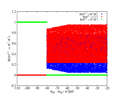
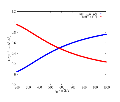
Figure 2: Distribution of various branching ratios of $H^{\pm\pm}$ decays.

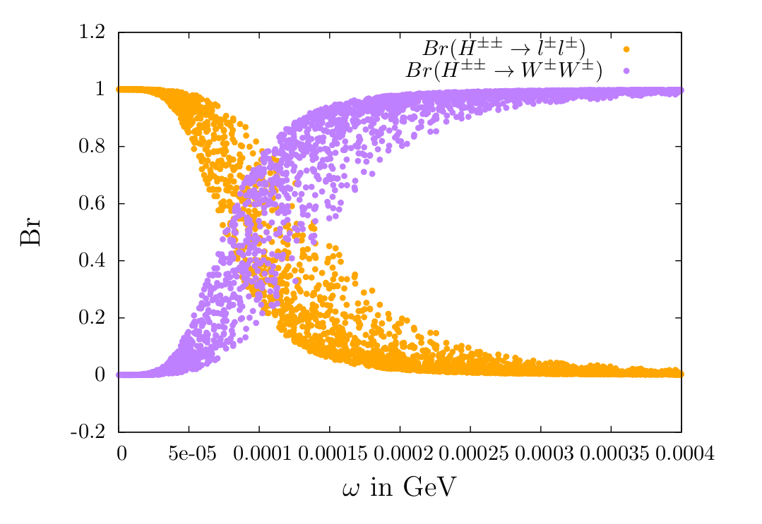
Figure 3: Branching fractions of doubly-charged Higgs decaying into $\ell^{\pm}\ell^{\pm}$ and $W^{\pm}W^{\pm}$ channels as a function of triplet VEV.

We have already seen that for $\omega<10^{-5}$ GeV, $Br(H^{\pm\pm}\rightarrow\ell^{\pm}\ell^{\pm})\simeq 100\%$ while for $\omega>10^{-4}$ GeV, $Br(H^{\pm\pm}\rightarrow W^{\pm}W^{\pm})\simeq 100\%$. In the intermediate region they are comparable with each other, and the branching ratio in either channel will depend on the mass of the doubly-charged Higgs. The right panel in Figure 2 describes the competition between the $Br(H^{\pm\pm}\rightarrow\ell^{\pm}\ell^{\pm})$ and $Br(H^{\pm\pm}\rightarrow W^{\pm}W^{\pm})$ as a function of $m_{H}^{\pm\pm}$ in such intermediate regions ($\omega\sim 10^{-4}$ GeV). It can be clearly seen that as $m_{H^{\pm\pm}}$ increases it favours $W^{\pm}W^{\pm}$ channel over $\ell^{\pm}\ell^{\pm}$ channel.

The doubly charged Higgs has been searched by ATLAS and CMS collaborations. The searches focus on $H^{\pm\pm}$ produced via DY process which is the only relevant channel. ATLAS have searched for the DY pair production of $H^{++}H^{--}$ with 36$fb^{-1}$ data at 13 TeV in $W^{\pm}W^{\pm}$ Aaboud:2018qcu and $\ell^{\pm}\ell^{\pm}$ Aaboud:2017qph channel. CMS have also looked for $H^{\pm\pm}\rightarrow\ell^{\pm}\ell^{\pm}$ in the $H^{++}H^{--}$ and $H^{\pm\pm}H^{\mp}$ final state with 12.9 $fb^{-1}$ data at 13 TeV CMS-PAS-HIG-16-036 . The search in the $W^{\pm}W^{\pm}$ channel puts a lower bound of $m_{H}^{\pm\pm}\raisebox{-3.69899pt}{~{}\shortstack{$<$ \\ [-0.07cm] $\sim$}}~{}220$ GeV. The lower limit on $m_{H^{\pm\pm}}$, from searches in the $\ell^{\pm}\ell^{\pm}$ final state depend on the Br($H^{\pm\pm}\rightarrow\ell^{\pm}\ell^{\pm}$). In Figure 4 we show the lower limit on the mass of doubly charged Higgs as function of Br($H^{\pm\pm}\rightarrow\ell^{\pm}\ell^{\pm}$). One can see from this figure that the lower limit on $m_{H}^{\pm\pm}$ ranges from $m_{H}^{\pm\pm}>550$ GeV for Br($H^{\pm\pm}\rightarrow\ell^{\pm}\ell^{\pm})\simeq 17\%$ to $m_{H}^{\pm\pm}>770$ GeV for Br($H^{\pm\pm}\rightarrow\ell^{\pm}\ell^{\pm})\simeq 100\%$.

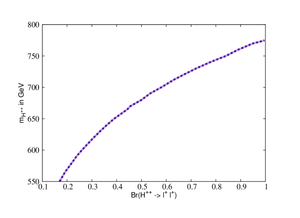
Figure 4: Experimental lower limit on $m_{H^{\pm\pm}}$ as a function of Br($H^{\pm\pm}\rightarrow\ell^{\pm}\ell^{\pm}$).

4.1 Same-sign dilepton channel

We first look for benchmarks for the case where $H^{\pm\pm}$ is best looked for in the same-sign dilepton final state. We want to identify the regions of parameter space where one can get sizable signal events in the decay channel that we are considering. It is clear from our previous discussion that the signal rate will be dependent on the product of three branching ratios, namely Br($H^{\pm\pm}\rightarrow\ell^{\pm}\ell^{\pm}$), $Br(H^{\pm}\rightarrow HW^{\pm})$ and Br($H\rightarrow invisible)$. It is clear from Figure 3 that $\omega\leq$ 0.0005 GeV Br$(H^{\pm\pm}\rightarrow\ell^{\pm}\ell^{\pm})>90\%$. We have noticed that when the mass gap between $H^{\pm}$ and $H$ exceeds $m_{W}$, $H^{\pm}$ goes to $HW^{\pm}$ with 50% branching as long as $\omega$ is very small. This is because, triplet VEV and correspondingly doublet-triplet mixing being small, additional channels such as $H^{\pm}\rightarrow hW^{\pm}$, $H^{\pm}\rightarrow W^{\pm}Z$ and $H^{\pm}\rightarrow t\bar{b}$ do not open up. In Figure 5 we show Br($H\rightarrow\chi\chi$) as a function of triplet VEV and also compare it with Br($H^{\pm\pm}\rightarrow\ell^{\pm}\ell^{\pm}$). We can see that Br($H\rightarrow\chi\chi$) increases with increasing triplet VEV whereas $Br(H^{\pm\pm}\rightarrow\ell^{\pm}\ell^{\pm}$) decreases with it. Typically one can choose some intermediate $\omega\in[10^{-5},10^{-4}]$ to get moderately good branching ratios in both these channels at the same time. We also notice that unless the mixing between the doublet and triplet CP-even scalar states is extremely small, the $H$ goes primarily to a pair of $hh$ and consequently Br($H\rightarrow\chi\chi$) becomes very small. The dependence of Br($H\rightarrow\chi\chi$) on the mixing angle $\alpha$ is shown in Figure 6. Therefore to get considerable branching in the $H\rightarrow\chi\chi$ channel, we have taken the mixing to be very small, ie. $\sin\alpha\sim 1$.

One should be careful while calculating the invisible decay width of heavy Higgs in this case, since $H$ can go to a pair of neutrinos or antineutrinos when the lepton flavor violating yukawa coupling is large enough. That will also contribute to invisible decay of the heavy Higgs. Br($H\rightarrow\nu\nu/\bar{\nu}\bar{\nu}$) has same dependence on $\omega$ as Br($H^{\pm\pm}\rightarrow\ell^{\pm}\ell^{\pm}$), because they are governed by the same yukawa coupling. We will consider Br_invisible of heavy Higgs to be the sum of Br($H\rightarrow\chi\chi$) and Br($H\rightarrow\nu\nu/\bar{\nu}\bar{\nu}$). We have chosen our benchmark points in a way to encompass different scenarios. We have chosen two cases (BP1 and BP2). In BP 1 Br($H\rightarrow\nu\nu/\bar{\nu}\bar{\nu}$) dominates over Br($H\rightarrow\chi\chi$), and in BP 2 they are comparable and we have tried to see whether these two cases can be distinguished. For comparison we have kept $m_{H}$ in a similar region in the two cases. We choose a third benchmark (BP 3) with lower $m_{H}$ and chosen $\omega$ in such a way that Br($H\rightarrow\chi\chi$) dominates over Br($H\rightarrow\nu\nu/\bar{\nu}\bar{\nu}$). In this case although the total branching in the specific decay mode will be less, the low mass of $H$ will enable us to get larger production cross section and in turn can be probed at the LHC.

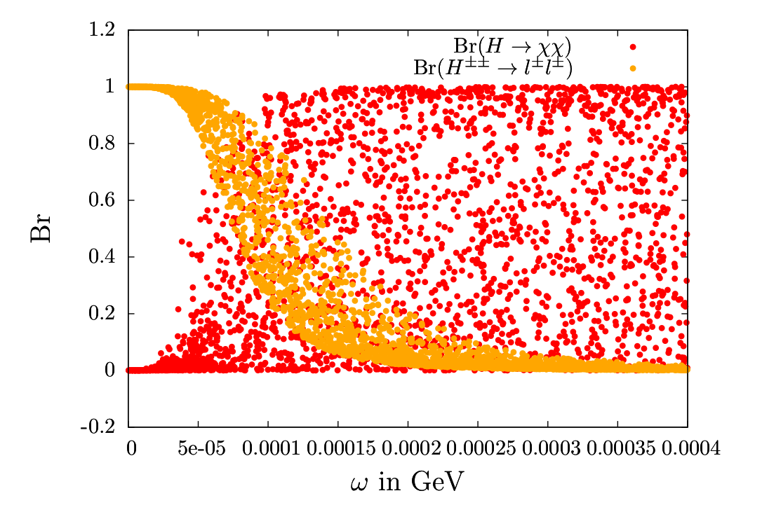
Figure 5: Distribution of various branching ratios as a function of $\omega$.

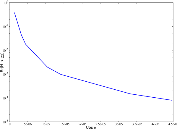
Figure 6: Br($H\rightarrow\chi\chi$) as a function of the mixing angle.

We define a new parameter $Br_{total}^{\ell\ell}=Br(H^{\pm\pm}\rightarrow\ell^{\pm}\ell^{\pm})\times Br(H^{\pm}\rightarrow W^{\pm}H)\times Br(H\rightarrow invisible)$ and search for moderate to large values of this quantity throughout our allowed parameter space. In Figure 7 we plot $Br_{total}^{\ell\ell}$ as a function of $m_{H}$. The orange region satisfy all the constraints except direct detection. The brown points satisfy the direct detection constraints along with all other constraints discussed above. We present our benchmark choices governed by the discussion above in Table 1. We have checked that they obey all the constraints discussed in Section 3, including the relic density suggested by the Planck data at $2\sigma$ level..

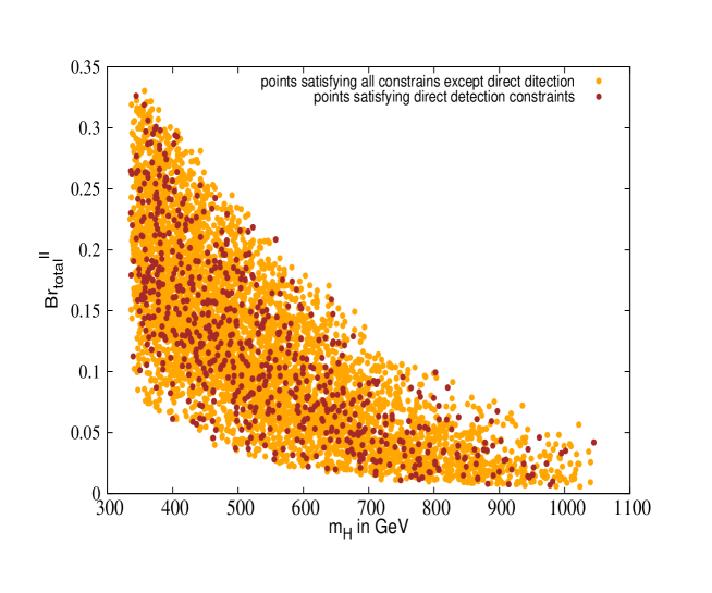
Figure 7: $m_{H}$ distribution of $Br_{total}^{\ell\ell}$. Orange points satisfy only relic density bounds and over and above that the brown points satisfy the current direct detection limit coming from XENON1T.

	BP 1	BP 2	BP 3
$m_{H}$ in GeV	423.1	615.1	615.1
$m_{A}$ in GeV	423.1	615.1	615.1
$m_{H^{\pm}}$ in GeV	509.3	697.0	697.0
$m_{H^{\pm\pm}}$ in GeV	582.8	770.0	770.0
$m_{\chi}$ in GeV	59.3	56.4	56.4
$\lambda_{S}$	0.49	0.0297	-0.0297
$\lambda_{D}$	0.00069	0.002125	0.002125
$\lambda_{T}$	11.258	10.51	10.51
$\omega$ in GeV	1.348$\times 10^{-4}$	4.074$\times 10^{-5}$	7.274$\times 10^{-5}$
$\sigma(pp\rightarrow H^{\pm\pm}H^{\mp})$ in $fb$	1.19	0.43	0.43
$Br(H\rightarrow invisible)$	0.92	0.935	0.79
$Br(H^{\pm\pm}\rightarrow\ell^{\pm}\ell^{\pm})$	0.228	0.95	0.65
$Br_{total}$	0.1049	0.44365	0.25675

Table 1: The Benchmark points for same-sign dilepton channel.

4.2 Same-sign vector boson ($W^{\pm}W^{\pm}$) channel

We turn next to the other important decay mode of $H^{\pm\pm}$, namely, a pair of same-sign $W$ bosons, which will give rise to different signature. In Figure 8 we present the comparison between $Br(H^{\pm\pm}\rightarrow W^{\pm}W^{\pm}$) and $Br(H^{\pm\pm}\rightarrow\chi\chi$), the two relevant branching fractions in this case. We can see here that Br$(H^{\pm\pm}\rightarrow W^{\pm}W^{\pm})$ increases with $\omega$ and becomes nearly 100% for $\omega\raisebox{-3.69899pt}{~{}\shortstack{$>$ \\ [-0.07cm] $\sim$}}~{}10^{-4}$ GeV. This is because when the triplet VEV increases beyond this value, $Br(H^{\pm\pm}\rightarrow\ell^{\pm}\ell^{\pm})$ becomes very low due to suppression in the lepton number violating Yukawa coupling and therefore the $W^{\pm}W^{\pm}$ channel takes over. As a consequence of the concomitantly suppressed lepton number violating Yukawa coupling $Br(H\rightarrow\nu\nu/\bar{\nu}\bar{\nu})$ also decreases significantly and therefore the heavy Higgs dominantly goes into the $\chi\chi$ channel. Thus in Figure 8 both $Br(H^{\pm\pm}\rightarrow W^{\pm}W^{\pm})$ and $Br(H^{\pm\pm}\rightarrow\chi\chi)$ both increase as $\omega$ increases. A notable point here is that in this region with larger triplet VEV, the invisible branching ratio of $H$ will consist of $H\rightarrow\chi\chi$ channel overwhelmingly, because of negligible branching fraction of $H$ in the $\nu\nu/\bar{\nu}\bar{\nu}$ channel.

While choosing benchmarks for our collider analysis we keep in mind the extremely low leptonic branching ratio of the same-sign $W$ pair. Therefore to get sufficient event rate we have chosen mass of $H$ to be on the lower side (220-400 GeV) which are consistent with the experimental searches. In BP 1 $m_{H}$ has been chosen to be $\simeq 220$ GeV. In BP 2 and BP 3 we take $m_{H}$ in a slightly higher range around $300-400$ GeV. When the triplet VEV is small and correspondingly the doublet-triplet mixing is also low, the decay modes $H^{\pm}\rightarrow hW^{\pm}$, $H^{\pm}\rightarrow W^{\pm}Z$ and $H^{\pm}\rightarrow t\bar{b}$ are not accessible. Hence $Br(H^{\pm}\rightarrow HW^{\pm}$) and $Br(H^{\pm}\rightarrow AW^{\pm}$) become the two dominant decay channels, each about 50% branching ratio as was discussed in the previous subsection. But as the triplet VEV increases, doublet-triplet mixing also goes up and the modes $H^{\pm}\rightarrow hW^{\pm}$, $H^{\pm}\rightarrow W^{\pm}Z$ and $H^{\pm}\rightarrow t\bar{b}$ open

Figure 8: Distribution of various branching ratios as a function of triplet VEV.

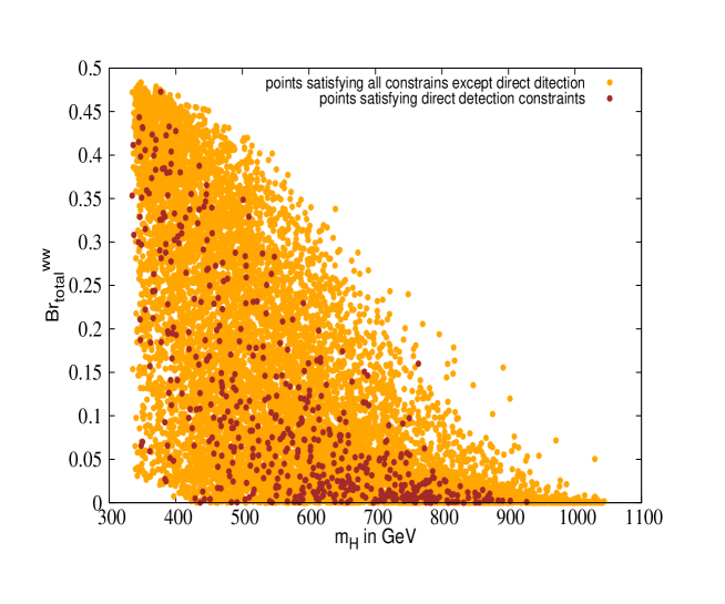
Figure 9: $m_{H}$ distribution of Br${}_{total}^{WW}$. Orange points satisfy only relic density bounds and over and above that the brown points satisfy the current direct detection limit coming from XENON1T.

	BP 1	BP 2	BP 3
$m_{H}$ in GeV	220.0	300.0	400.0
$m_{A}$ in GeV	220.0	300.0	400.0
$m_{H^{\pm}}$ in GeV	301.0	382.0	482.0
$m_{H^{\pm\pm}}$ in GeV	371.0	451.0	551.0
$m_{\chi}$ in GeV	57.6	125.0	180.1
$\lambda_{S}$	0.0472	0.0725	0.0264
$\lambda_{D}$	0.00156	0.00862	0.0256
$\lambda_{T}$	8.67	5.3938	8.981
$\omega$ in GeV	0.1034	4.68	0.261
$\sigma(pp\rightarrow H^{\pm\pm}H^{\mp})$ in $fb$	16.2	6.7	2.5
$Br(H\rightarrow invisible)$	0.99	0.89	0.82
$Br(H^{\pm}\rightarrow W^{\pm}H)$	0.50	0.30	0.50
$Br(H^{\pm\pm}\rightarrow W^{\pm}W^{\pm})$	1.0	1.0	1.0
$Br_{total}$	0.49	0.27	0.41

Table 2: The Benchmark points for same-sign $W$ channel.

up with considerable branching fractions. Consequently, $Br(H^{\pm}\rightarrow HW^{\pm}$) falls. In BP 2 we have considered such a situation with $\omega$ close to its allowed upper limit. In this case $Br(H^{\pm}\rightarrow HW^{\pm})$ comes down to 30% (see Table 2).

In Figure 9 we plot the quantity $Br_{total}^{WW}$ analogous to $B_{total}^{\ell\ell}$ as defined in the previous subsection, as a function of $m_{H}$ when the $W^{\pm}W^{\pm}$ decay mode of the doubly charged Higgs becomes dominant. The three benchmark points, used in our study of the $W^{\pm}W^{\pm}$-driven final state, are shown in Table 2. Once more, these are consistent with all constraints including those from the observed relic density.

5 Collider Analysis (Cut based)

From the discussion of the previous section, we are convinced that the heavy neutral Higgs can serve as a dark matter portal in a Type-II Seesaw scenario with a singlet scalar DM particle. Our goal at this point is to look for signatures of this model in the channels already discussed in the previous section, and explore their reach at the high-luminosity run of the LHC. In this spirit, we consider in turn cases where the heavy CP-even Higgs ($H$) can decay into a pair of dark matter with substantial branching fraction. Obviously, the events will consist of large $\not{E_{T}}$. As mentioned already, production of $H$ can be significant only through Drell-Yan processes. Hence we concentrate on (i) $pp\rightarrow H^{\pm\pm}H^{\mp},H^{\pm\pm}\rightarrow\ell^{\pm}\ell^{\pm},H^{\pm}\rightarrow HW^{\pm},H\rightarrow invisible$, and (ii) $pp\rightarrow H^{\pm\pm}H^{\mp},H^{\pm\pm}\rightarrow W^{\pm}W^{\pm},H^{\pm}\rightarrow HW^{\pm},H\rightarrow invisible$. These two channels are somewhat complementary in nature, having significant rates in different regions of the parameter space. We will henceforth call the first scenario Case I, and second one, Case II. As has been stated in the introduction, we have also considered the $W$-boson fusion process, namely, $pp\rightarrow H^{\pm\pm}H+\text{two forward jets}$ after which $H$ decays into invisible final states. However, this process will have irreducible background from SM VBF production and will not have enough signal rate even at the high-luminosity(HL) LHC. Thus we will concentrate on the DY-production of $H$ with final states pertaining to the two major decay modes of $H^{\pm\pm}$, namely, $\ell^{\pm}\ell^{\pm}$ and $W^{\pm}W^{\pm}$. We will briefly comment on the $W$-fusion channel at the end of this section.

Events for the signals and their corresponding backgrounds have been generated using Madgraph@MCNLO Alwall:2014hca and their cross-sections have been calculated at the next-to-leading order(NLO). We take the renormalization and factorization scales at the $p_{T}$ of the hardest jet and also use the nn23lo1 parton distribution function. At the NLO level, the results with other scale choices do not differ by more than ($10\%$). PYTHIA8 Sjostrand:2006za has been used for the showering and hadronization and the detector simulation has been taken care of by Delphes-3.4.1 deFavereau:2013fsa .

5.1 Case I

The Drell-Yan production of $H^{\pm\pm}H^{\mp}$ will lead to the final state containing a pair of same-sign dilepton from the decay of $H^{\pm\pm}$. The $H^{\pm}$ will decay into $W^{\pm}$ and $H$ wherever this decay is kinematically allowed . The invisible decay of $H$ will lead to $\not{E_{T}}$ in the final state. We have considered only hadronic decays of $W^{\pm}$ to have sizable number of events in the signal process. The same-sign dilepton pair constitutes a clean signal to look for in experiments.

Signal: The signal here is a pair of same-sign leptons ($e/\mu$) + 2 jets + $\not{E_{T}}$. This signal has been searched for in the LHC Khachatryan:2016kod . It reports no significant excess over the SM expectation with $\int{\cal L}dt=36fb^{-1}$ at 95% C.L. .

Background: The dominant backgrounds for this final state are Khachatryan:2016kod

• $t\bar{t}$ semileptonic decay which leads to non-prompt leptons in the final state. Non-prompt leptons are those which can arise from heavy flavor decay or hadrons being misidentified as leptons etc.

• $W$ + jets also contributes to the background producing non-prompt leptons.

• $t\bar{t}W^{\pm}$ with semileptonic decay of $t\bar{t}$ which directly produces same-sign dilepton background is another background.

• $W^{\pm}Z$ with leptonic decay of $W^{\pm}$ and $Z$ also produces same-sign dilepton pairs and therefore is an important background for our signal.

• Charge misidentification: The charge misidentification probability for $e^{\pm}e^{\pm}$ lies in the range $10^{-5}-10^{-3}$ Khachatryan:2016kod depending on the $p_{T}$ and $\eta$. For muons charge misidentification probability is negligible Khachatryan:2016kod . This background thus does not play any significant role in the analysis.

5.1.1 Distributions

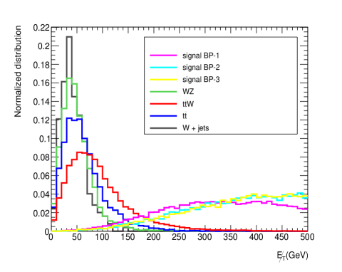
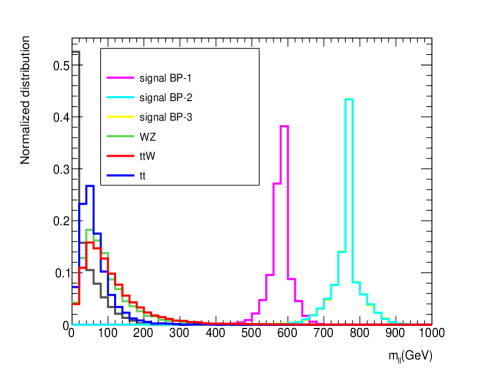
Figure 10: Distribution of $\not{E_{T}}$(left) and invariant mass(right) of same-sign dileptons for the three signal BPs and backgrounds in case I.

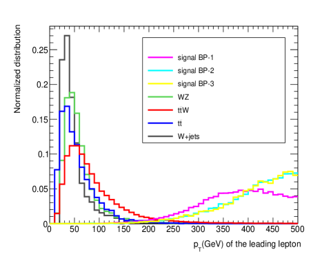
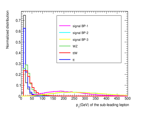
Figure 11: Distribution of transverse momenta of the leading(left) and sub-leading(right) leptons for the three signal BPs and backgrounds in case I.

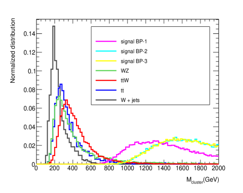
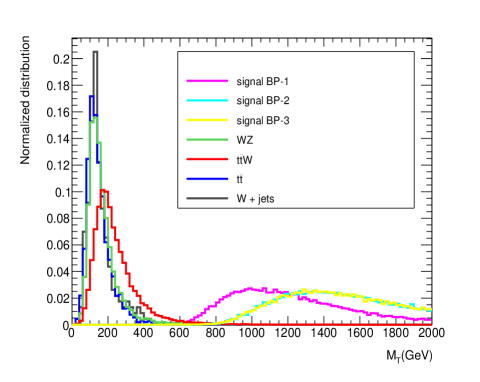
Figure 12: Distribution of cluster transverse mass(left) and transverse mass(right) for the three signal BPs and backgrounds in case I.

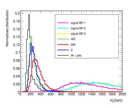
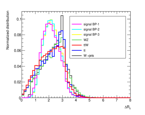
Figure 13: Distribution of $H_{T}$ and $\Delta R$ between leading and sub-leading leptons for the three signal BPs and backgrounds in case I.

We present various kinematic distributions for the signal and background processes. In Figure 10 (left), we plot the $\not{E_{T}}$ and invariant mass of the same-sign dilepton pair. The $\not{E_{T}}$ in the signals peaks at a higher value than that of the backgrounds since the $\not{E_{T}}$ in the signal comes from the invisible decay of a heavy Higgs. For BP 2 and 3 the $\not{E_{T}}$ peaks at a higher value as compared to BP 1, because of the higher mass of $H$ in the former case. The fact that the invariant mass of the same-sign dilepton peaks at $m_{H^{\pm\pm}}$ adds to the distinctness of the events, as can be seen in Figure 10 (right).

In Figure 11 we present the $p_{T}$ distributions of the leading and sub-leading leptons of the same-sign dilepton pair. The $p_{T}$ of the leptons in case of signal is much larger than that of the backgrounds as the dilepton pair in the signal process comes from the decay of a heavy doubly-charged Higgs. These, along with the observables mentioned in the previous paragraph, serve well to discriminate the signal from backgrounds.

Next come three observables which are related to each other. They are cluster transverse mass ($M_{cluster}$), transverse mass ($M_{T}$) and scalar $p_{T}$ sum ($H_{T}$), being defined as Han:2007bk

$$M_{cluster}=\sqrt{m^{2}_{2j}+(\sum{\vec{p_{T}}^{j}})^{2}}+\sqrt{m^{2}_{\ell\ell}+(\sum{\vec{p_{T}}^{\ell}})^{2}}+\not{E_{T}}$$ (38)

$$M_{T}=\sqrt{(\sqrt{m^{2}_{\ell\ell}+(\sum{\vec{p_{T}}^{\ell}})^{2}}+\not{E_{T}})^{2}}-(\sum{\vec{p_{T}}^{\ell}}+\vec{\not{E_{T}})^{2}}.$$ (39)

and

$$H_{T}=(\sum{{p_{T}}^{j}})+(\sum{{p_{T}}^{\ell}})+\not{E_{T}}$$ (40)

respectively.

From Equations. 38, 39 and  40 we can see that $m_{cluster}$ represents the sum of $p_{T}$ of the dilepton and jets system, invariant mass of the dilepton and the jets system and $\not{E_{T}}$. $M_{T}$ represents the sum of $p_{T}$ of the dilepton system, invariant mass of the dilepton system and $\not{E_{T}}$. $H_{T}$, on the other hand is the scalar sum of the transverse momenta of all the final state particles. As Table 3 shows, cuts on these variables have practically the same efficiency as far as the signal is concerned, while they affect the background a little differently from each other. While they have been applied in succession in the cut-based analysis reported here, they have been retained in the subsequent neural network analyses too, where their correlation is duly taken into account.

From Figure 12 (left) it can be seen that the distribution in the cluster transverse mass for the whole system for the signal peaks at a higher value than that of the background. The $M_{T}$-distribution in the right panel shows a similar trend. Figure 13 (left) shows the $H_{T}$-distributions, once more with the same trend, as expected. This common feature of all three observables is there because of higher $p_{T}$ for the leptons as well as the harder $\not{E_{T}}$-distribution of the signal compared to the background. These characteristics percolate through all three variables, and, albeit in a correlated fashion, constitute important inputs in a neural network analysis, as will be reported later in this paper.

We next consider the isolation $\Delta R(=\sqrt{\Delta\eta^{2}+\Delta\phi^{2}}$) between the two leptons. From Figure 13 (right) it can be seen the peaks for signal processes are at a lower value than that of the backgrounds. The signal dileptons come from the $H^{\pm\pm}$ and thus have a higher probability of being in the same hemisphere, than in the case of the dominant background channels. However, the $H^{\pm\pm}$ produced in a Drell-Yan process is devoid of large boost, thus preventing the aforesaid isolation from being a very good discriminator. It nonetheless has a role in the neural network analysis.

It is relevant to mention here that the above kinematic distributions for BP 2 and 3 look quite similar. The reason behind this is, in both the cases the mass of the heavy Higgs states are same. On the one hand, the lepton hardness level is controlled by the $m_{H^{\pm\pm}}$. On the other side, $\not{E_{T}}$, too, is decided by $m_{H}$, though the invisible decay of the latter takes place in different final states for the two benchmark points; for BP 2 it is $H\rightarrow\nu\nu$, and $H\rightarrow\chi\chi$ for BP 3.

5.1.2 Results

Based on the preceding observations, we have applied the following cuts on the observables. The events selected will have at least two jets and two same-sign dileptons($e/\mu$). The leptonic decay of $\tau$ has not been considered since its contribution is rather small.

• Cut 1: The invariant mass of the same-sign dileptons $m_{ll}>400$ GeV.

• Cut 2: Cluster transverse mass $M_{cluster}>700$GeV.

• Cut 3. Scalar $p_{T}$ sum $H_{T}>$ 700 GeV.

• Cut 4: Transverse mass $M_{T}>$ 550 GeV.

• Cut 5: $\not{E_{T}}>300$ GeV.

• Cut 6: $p_{T}$ of the leading lepton $>250$ GeV and $p_{T}$ of the sub-leading lepton $>200$ GeV.

	BP 1	BP 2	BP 3	$t\bar{t}$	$W$ + jets	$t\bar{t}W$	WZ
$\sigma(fb)$	0.12	0.19	0.11	$3.09\times 10^{5}$	$2.8\times 10^{7}$	9.77	355.10
Cut 1	99.3%	99.6%	99.6%	0.2%	0.15%	2.1%	1.8%
Cut 2	99.2%	99.6%	99.6%	0.1%	0.08%	1.7%	1.3%
Cut 3	96.8%	99.2%	99.1%	0.06%	0.03%	0.9%	0.4%
Cut 4	96.8%	99.2%	99.1%	0.05%	0.026%	0.8%	0.3%
Cut 5	73.5%	87.4%	87.6%	$0.01$%	0.003%	0.07%	0.04%
Cut 6	40.2%	62.5%	62.4%	$0.002$%	0.0009%	0.01%	0.005%

Table 3: Signal and background efficiencies after applying various cuts for case I at 14 TeV. The cross-sections are calculated at NLO.

Table 3 shows the cut-flow for the signal and the background for case I, yielding a fair indication of the efficiency of each cut. In Table 4 we calculate the projected significance (${\cal S})$ for each benchmark point for the 14 TeV LHC with 3000 $fb^{-1}$. The significance ${\cal S}$ is defined as

$${\cal S}=\sqrt{2[(S+B)\text{Log}(1+\frac{S}{B})-S]}$$ (41)

Where $S$ and $B$ are the number of signal and background events surviving the succession of cuts.

BP	${\cal S}$
BP 1	3.4 $\sigma$
BP 2	8.3 $\sigma$
BP 3	5.0 $\sigma$

Table 4: Signal significance for the benchmark points at 14 TeV with ${\cal L}$ = 3000 $fb^{-1}$ for case I.

We can see from Table 4 that for BP 2 the largest significance is predicted. Although in BP 2 the production cross-section for $H^{\pm\pm}H^{\mp}$ is smaller compared to that in BP 1, BP 2 has large invisible branching ratio(mostly $H\rightarrow\nu\nu$) as well as large Br($H^{\pm\pm}\rightarrow\ell^{\pm}\ell^{\pm}$) since it corresponds to the smallest triplet VEV among the three benchmarks. On the other hand, BP 1 has smaller Br($H^{\pm\pm}\rightarrow\ell^{\pm}\ell^{\pm}$) because of larger triplet VEV, and consequently smaller $\Delta L=2$ interaction strengths (in order to conform to the neutrino mass limits). Therefore, even with large invisible branching fraction for $H\rightarrow\chi\chi$ this BP suffers from lower overall rate. In case of BP 3, Br($H\rightarrow\chi\chi$) and Br($H\rightarrow\nu\nu$) are comparable, the smaller Br($H^{\pm\pm}\rightarrow\ell^{\pm}\ell^{\pm}$) due to smaller triplet VEV makes this BP a little more challenging than BP 2 from the experimental point of view. Moreover, the masses of the heavy states $H^{\pm\pm},H^{\pm}$ and $H$ are larger in BP 2 and 3, as compared to BP 1. Thus one has better handle on the signal separation process, using the variables discussed already.

5.2 Case II

For relatively large ($\raisebox{-3.69899pt}{~{}\shortstack{$>$ \\ [-0.07cm] $\sim$}}~{}10^{-3}$ GeV) triplet VEV, the $H^{\pm\pm}$ produced in the Drell-Yan process will decay into a pair of same-sign $W$ bosons. The leptonic decay of the produced $W$-bosons once more gives rise to same-sign dileptons along with $\not{E_{T}}$, but without any dilepton invariant mass peak. It is profitable to latch on to hadronic decays of the $W$ coming from the associated $H^{\pm}$ decaying into $HW^{\pm}$ final state. When the above decay is kinematically suppressed, the $H^{\pm}$ will decay into $W^{\pm}h$ or $W^{\pm}Z$ final states, empowered by the relatively higher triplet VEV. The subsequent invisible decay of $H$ will be a tell-tale signature of dark matter, the $\nu\nu$ mode being suppressed by the Yukawa coupling in this case.

The sources of backgrounds here are the same as in case I. However, the fact that same-sign dileptons in this case do not come from a single source causes somewhat different kinematical features compared to case I, as we will see below.

5.2.1 Distributions

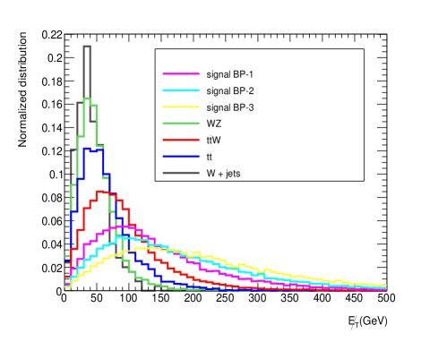
Figure 14: Distribution of $\not{E_{T}}$(left) and invariant mass(right) of same-sign dileptons for the three signal BPs and backgrounds in case II.

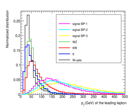
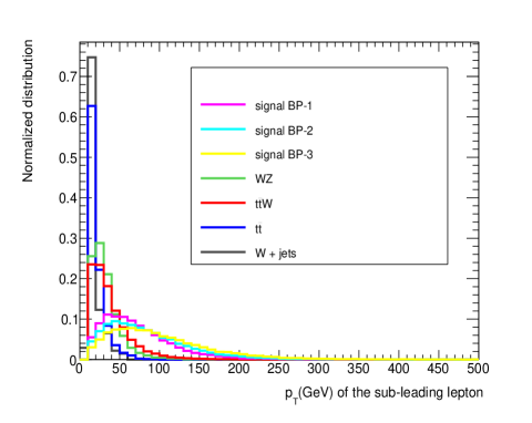
Figure 15: Distribution of transverse momenta of the leading(left) and sub-leading(right) leptons for the three signal BPs and backgrounds in case II.

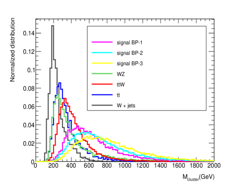
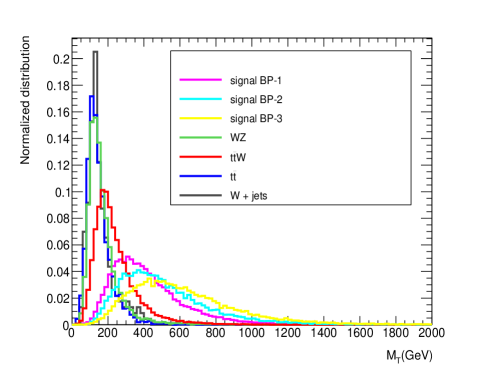
Figure 16: Distribution of cluster transverse mass(left) and transverse mass(right) for the three signal BPs and backgrounds in case II.

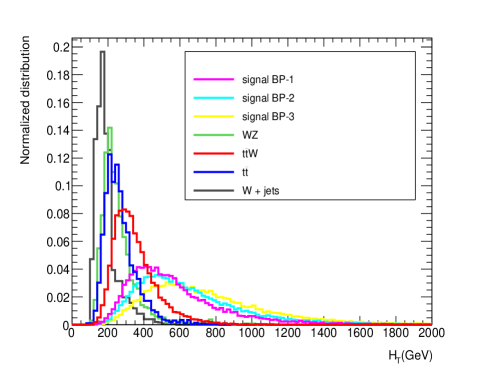
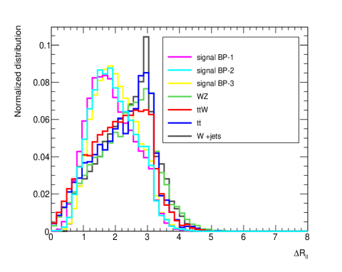
Figure 17: Distribution of $H_{T}$ and $\Delta R$ between leading and sub-leading leptons for the three signal BPs and backgrounds in case II.

In Figure 14 (left) we plot the $\not{E_{T}}$ distribution in the final state. We can see that for the signal processes, the distribution peaks at lower values than case I even when masses of heavy Higgses are in similar regions. This is because the source of neutrinos here are the two boosted same-sign $W$-bosons, which occur in the hemisphere opposite to the one where the $H$ emanates, thus enabling the cancellation of missing transverse momenta.

Figure 14 (right) shows the invariant mass distribution of the same-sign dilepton pair. The peak in this distribution also shifts to a lower value compared to case I, largely because of the reduced individual energy share of each participating lepton. The signal $p_{T}$ distributions, too, peak at a lower values compared to case I, as seen in Figure 14. A similar fate also awaits $M_{cluster},M_{T}$ and $H_{T}$, as seen from Figures 16 and 17. Along with similar, and less consequential isolations as in Figure 17 (right), these features make the statistical significance relatively modest in Case II.

5.2.2 Results

Gaining some insight into the kinematics of the final state particles in signal and background processes, we apply various cuts on the relevant observables and perform a cut-based analysis. The events with exactly two same-sign dileptons and at least two jets are selected. The following cuts have been applied in succession on both signal and background events.

• Cut 1: The invariant mass of the same-sign dileptons $m_{ll}>150$ GeV.

• Cut 2: Cluster transverse mass $M_{cluster}>500$GeV.

• Cut 3. Scalar $p_{T}$ sum $H_{T}>$ 500 GeV.

• Cut 4: Transverse mass $M_{T}>$ 500 GeV.

• Cut 5: $\not{E_{T}}>250$ GeV.

• Cut 6: $p_{T}$ of the leading lepton $>200$ GeV and $p_{T}$ of the sub-leading lepton $>100$ GeV.

	BP 1	BP 2	BP 3	$t\bar{t}$	$W$ + jets	$t\bar{t}W$	$WZ$
$\sigma(fb)$	0.79	0.18	0.10	$3.09\times 10^{5}$	$2.8\times 10^{7}$	9.77	355.10
Cut 1	62.0%	77.0%	88.0%	4.8%	3.1%	28.2%	24.4%
Cut 2	47.0%	64.0%	78.2%	3.0%	1.8%	18.2%	11.2%
Cut 3	39.0%	55.0%	70.0%	0.7%	0.42%	12.0%	4.0%
Cut 4	23.0%	39.0%	57.3%	0.2%	0.1%	4.0%	1.4%
Cut 5	8.8%	20.0%	31.8%	0.04%	0.014%	0.8%	0.3%
Cut 6	4.7%	10.0%	17.2%	0.01%	0.004%	0.1%	0.05%

Table 5: Signal and background efficiencies after applying various cuts for case II at 14 TeV. The cross-sections are calculated at NLO.

In Table 5 we present the cut-flow for signal and backgrounds for case II. Finally, Table 6 contains the projected signal significance for the three benchmarks for 14 TeV LHC with 3000 $fb^{-1}$ data. The significance ${\cal S}$ is defined in Equation 41.

BP	${\cal S}$
BP 1	2.0 $\sigma$
BP 2	1.0 $\sigma$
BP 3	1.1 $\sigma$

Table 6: Signal significance for the benchmark points at 14 TeV with ${\cal L}$ = 3000 $fb^{-1}$ for case II.

We can see from Table 6 that only BP 1 will have substantial significance at 3000 $fb^{-1}$ luminosity. The major reason behind that is large production cross-section helped by comparatively low heavy Higgs masses. Moreover, this benchmark also has all relevant branching fractions, namely, those for $H\rightarrow\chi\chi,H^{\pm}\rightarrow HW^{\pm}$ and $H^{\pm\pm}\rightarrow W^{\pm}W^{\pm}$, working in favour of the signal. It has Br($H\rightarrow\chi\chi\approx 90\%$). On the other hand, BP 1 has the lowest triplet VEV among the three BPs. In this case $H^{\pm}$ decays mostly to $HW^{\pm}$ final state. For BP 2, however, other decay channels like $hW^{\pm},t\bar{b}$ etc open up, hence the Br$(H^{\pm}\rightarrow HW^{\pm}$) falls (27% in case of BP 2 as this channel has the largest VEV). Therefore, although BP 2 and 3 have better separation between signal and background owing to large heavy Higgs masses, the low cross-sections and branching fractions make such regions in the parameter space somewhat challenging. Keeping this in mind, the remaining part of our investigation goes beyond rectangular cuts.

5.3 W-boson fusion

As an alternative channel, one may think of $W$-boson fusion, since it provides the useful forward jets tag. Here a relevant production channel could be $pp\rightarrow H^{\pm\pm}H$ + two forward jets along with $H$ decaying into the invisible channel, and leading to same-sign dilepton + $\not{E_{T}}$ in the rapidity interval between the forward jets. On actual calculation, however, it is found that even the most optimistic benchmarks lead to production cross-section $\approx 10^{-2}fb$. The event rate after factorizing in the decay branching ratios and applying various selection criteria thus becomes rather small even for the HL-LHC. We therefore do not enter into detailed analysis of this channel.

6 Results with gradient boosting and neural networks

Having performed the rectangular cut-based analysis for same-sign dilepton + $\not{E_{T}}$ signal, we see that some benchmark points yield very good signal significance at the HL-LHC. Therefore they will be easily detectable at the future run. However, there are some benchmarks which predict rather poor signal significance in a cut-based analysis. Specifically, BP 2 and 3 of the scenario with $H^{\pm\pm}\rightarrow W^{\pm}W^{\pm}$ yield very low significance, as seen in Table 6. The main reason behind this is the comparatively low production cross-section and branching ratio in this case. Moreover, the absence of a same-sign dilepton peak makes it somewhat challenging in case II. Taking this issue into consideration we move towards a more sophisticated analysis using packages based on Gradient boosting (XGBoost) Chen:2016btl and Artificial neural network (ANN) Teodorescu:2008zzb techniques. Their usefulness has been widely demonstrated Baldi:2014kfa ; Woodruff:2017geg ; Oyulmaz:2019jqr ; Bhattacherjee:2019fpt including studies in the Higgs sector Hultqvist:1995ibm ; Field:1996rw ; Bakhet:2015uca ; Dey:2019lyr ; Lasocha:2020ctd . In this section we will explore the possibility of improvement of our analysis using these techniques. In particular for ANN we have used the toolkit Keras keras . We perform the analysis for both case I and II and also make a comparative study of the performance of ANN and XGBoost in the two cases. In Table 7 we list all relevant variables these being a total of 12 such feature variables in the analysis.

Variable	Definition
$P^{l_{1}}_{T}$	Transverse momentum of the leading lepton
$P^{l_{1}}_{T}$	Transverse momentum of the sub-leading lepton
$E^{miss}_{T}$	Missing transverse energy
$N_{j}$	No of jets in the event
$m_{ll}$	Invariant mass of the same-sign dilepton pair
$P^{j_{1}}_{T}$	Transverse momentum of the leading jet
$P^{j_{1}}_{T}$	Transverse momentum of the sub-leading jet
$m_{jj}$	Invariant mass of the jets
$m_{cluster}$	The cluster transverse mass
$m_{transverse}$	Transverse mass
$H_{T}$	Scalar sum of $p_{T}$ of all the final state particles
$\Delta R_{ll}$	$\Delta R$ between two leptons

Table 7: Feature variables for training in the XGBoost and ANN analysis.

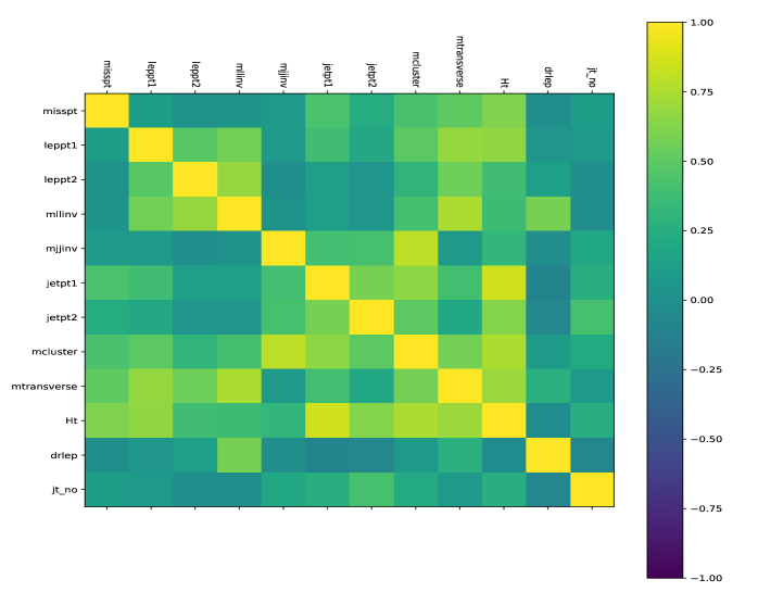
Figure 18: Correlation matrix between the feature variables using XGBoost.

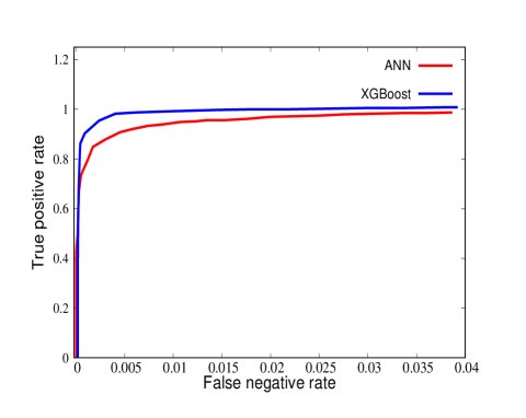
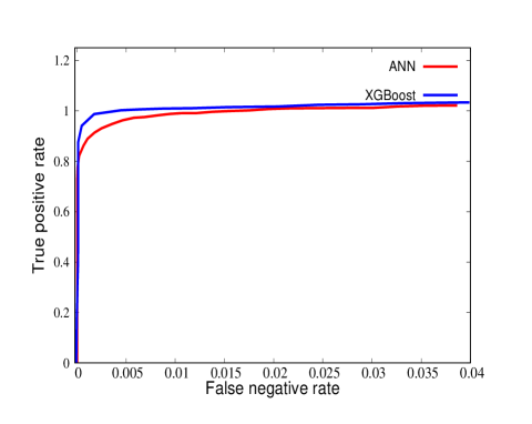
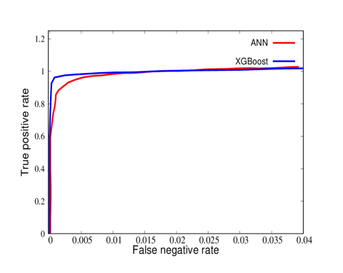
Figure 19: ROC curves of BP 1 (top left), BP 2 (top right) and BP 3 (bottom centre) in case I with ANN and XGBoost.

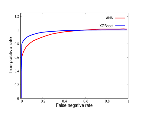
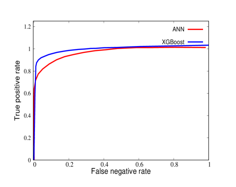
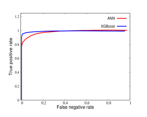
Figure 20: ROC curves of BP 1 (top left), BP 2 (top right) and BP 3 (bottom centre) in case II with ANN and XGBoost.

In the gradient boosted decision tree analysis we have used 1000 estimators, maximum depth 2 and a learning rate 0.02. In case of ANN we have used four hidden layers with activation curve tanh and relu in succession, a batch-size 200 for each epoch, and 100 such epochs. For both XGBoost and ANN analysis we have used 80% of the data for training and 20% for test or validation of the algorithm. We found out that in case I, the invariant mass of the same-sign dilepton pair plays the most important role in signal-background identification, $m_{transverse}$, $\not{E_{T}}$, $p_{T}$ of the leading and sub-leading leptons being of relatively lower importance. In case II, the invariant mass of the lepton pair becomes less relevant as we have discussed earlier. The most important observable in this case turns out to be $m_{transverse}$ including the correlated ones, namely $m_{cluster}$, $m_{transverse}$ $H_{T}$ as seen in Figures 18.

In Figure 19 and 20 we present the Receiver Operating Characteristic (ROC) curves for all the benchmarks of case I and II. For different scenarios and benchmarks considered here, the area under the ROC curves vary within the range 0.92-0.99. This implies that it is indeed possible to gain high signal selection efficiency with extremely low background selection. One possible issue with this kind of analyses is the possibility of over-training, in which case the separation between signal and background becomes extremely good for the training sample but for the test sample it fails to achieve the same level of distinction. We have explicitly checked that in our case the algorithm is not over-training, as a result of which the area under the curves remain almost same for training and test sample. In Figure 19 we can see that the large signal selection efficiency ($\sim 90$%) is achievable with extremely low background selection ($\sim 0.1$%) in case of all the BPs. The invariant mass of dilepton pair is the major reason behind such separation. For clarity we have plotted the background selection rate (false positive rate) upto a smaller range in this figure. In Figure 20 we can see that for signal selection efficiency ($\sim 90$%), one will have to allow $\sim 1$% fake background in case of $W^{\pm}W^{\pm}$ final state. Evidently the results will worsen as compared to $\ell^{\pm}\ell^{\pm}$ final state. One can also see from Figures 19 and 20, XGBoost performs slightly better than ANN in all cases, one deciding factor being the number of input variables Roe:2004na .

Next we compute the signal significance for all the benchmarks in case I and II with ANN and XGBoost. We present the results in Table 8 and 9 respectively. One can compare these results with the ones quoted in Table 4 and 6. It is clear that in all cases there is significant improvement from rectangular cut-based analysis. We particularly point out the BP 2 and 3 in case II. In these two cases we observe striking improvement from the cut-based results. Finding the best possible combination of feature variables to separate the signal and background ANN helps us improve the significance. On the other hand XGBoost does the same by choosing the best possible set of cuts on the most relevant observables. We remark here that the data sample used by us for training purpose may in principle be subjected to some pre-assigned additional cuts, such as demanding specific invariant masses for same-sign dileptons. Such a practice usually improves the signal significance furtherDey:2019lyr . We have desisted from using such cuts, since the significance is already quite impressive.

BP	${\cal S}$ (ANN)	${\cal S}$ (XGBoost)
BP 1	5.9 $\sigma$	7.8 $\sigma$
BP 2	9.3 $\sigma$	11.6 $\sigma$
BP 3	6.4 $\sigma$	7.9 $\sigma$

Table 8: Signal significance for the benchmark points at 14 TeV with ${\cal L}$ = 3000 $fb^{-1}$ for case I with ANN and XGBoost.

BP	${\cal S}$ (ANN)	${\cal S}$ (XGBoost)
BP 1	3.6 $\sigma$	4.8 $\sigma$
BP 2	3.9 $\sigma$	5.0 $\sigma$
BP 3	3.4 $\sigma$	4.0 $\sigma$

Table 9: Signal significance for the benchmark points at 14 TeV with ${\cal L}$ = 3000 $fb^{-1}$ for case II with ANN and XGBoost.

7 Conclusions

We use the fact that theories with extended scalar sectors can provide viable candidates for DM portal, avoiding the constraints prevailing on the SM Higgs from direct search and relic density considerations. Keeping this in mind, we have explored the scenario where a CP-even scalar from a triplet acts as the portal to the dark sector, consistently with the role of the triplet in the Type-II seesaw mechanism for neutrino mass generation. One can find interesting regions of the parameter space, which are consistent with all the requirements from Higgs data, dark matter experiments, precision measurement as well as theoretical constraints. We have chosen a few representative benchmark points which give significant production cross-section for the heavy Higgs bosons as well as branching ratios in the invisible channel for the heavy CP-even scalar $H$. The production of $H$ along with doubly charged Higgs has the advantage of same-sign dilepton in the final state, which is a clean signal to look for at the LHC. We have considered two complimentary scenarios with low and high triplet VEV, and explored the reach of the high-luminosity LHC in probing both cases. We have found out that choosing suitable kinematical observables it is possible to achieve significant event rates in both channels for specific benchmark points. The region with low triplet VEV provides us better signal-background separation, having the advantage of invariant mass peak for the same-sign dileptons. The region with moderate to large triplet VEV do not have this invariant mass peak as a discriminating variable. Also this channel suffers from low leptonic branching of the $W$ bosons. We ameliorate such difficulties by going beyond the rectangular cut-based analysis, applying gradient boosting as well as neural network techniques which strikingly improve the significance for all the scenarios.

It has been already mentioned in Section 4 that the signals considered here can be mimicked by a situation where the heavy triplet-dominated scalar $H$ has a substantial branching ratio into a pair of neutrinos, something that can be envisioned for small values of the triplet VEV. In principle, such a possibility can be distinguished by other collider signals of the Type-II Seesaw scenario, and from a relatively detailed understanding of its parameter space acquired thereby. In the (unlikely) case where such differentiation is impossible, searches for the signals suggested here will in any case serve to constrain a triplet DM portal.

8 Acknowledgement

We thank Asesh Krishna Datta for valuable comments. This work was supported by funding available from the Department of Atomic Energy, Government of India, for the Regional Centre for Accelerator-based Particle Physics (RECAPP), Harish-Chandra Research Institute. AD and JL thank Saha Institute of Nuclear Physics, Kolkata and Indian Institute of Science Education and Research Kolkata for hospitality, where substantial part of this work was done.

References

- (1) XENON collaboration, E. Aprile et al., Dark Matter Search Results from a One Ton-Year Exposure of XENON1T, Phys. Rev. Lett. 121 (2018) 111302, [1805.12562].
- (2) A. Drozd, B. Grzadkowski, J. F. Gunion and Y. Jiang, Extending two-Higgs-doublet models by a singlet scalar field - the Case for Dark Matter, JHEP 11 (2014) 105, [1408.2106].
- (3) A. Dey, J. Lahiri and B. Mukhopadhyaya, LHC signals of a heavy doublet Higgs as dark matter portal: cut-based approach and improvement with gradient boosting and neural networks, JHEP 09 (2019) 004, [1905.02242].
- (4) M. Magg and C. Wetterich, Neutrino Mass Problem and Gauge Hierarchy, Phys. Lett. 94B (1980) 61–64.
- (5) J. Schechter and J. W. F. Valle, Neutrino Masses in SU(2) x U(1) Theories, Phys. Rev. D22 (1980) 2227.
- (6) G. Lazarides, Q. Shafi and C. Wetterich, Proton Lifetime and Fermion Masses in an SO(10) Model, Nucl. Phys. B181 (1981) 287–300.
- (7) R. N. Mohapatra and G. Senjanovic, Neutrino Masses and Mixings in Gauge Models with Spontaneous Parity Violation, Phys. Rev. D23 (1981) 165.
- (8) T. P. Cheng and L.-F. Li, Neutrino Masses, Mixings and Oscillations in SU(2) x U(1) Models of Electroweak Interactions, Phys. Rev. D22 (1980) 2860.
- (9) S. M. Bilenky, J. Hosek and S. T. Petcov, On Oscillations of Neutrinos with Dirac and Majorana Masses, Phys. Lett. 94B (1980) 495–498.
- (10) I. Yu. Kobzarev, B. V. Martemyanov, L. B. Okun and M. G. Shchepkin, THE PHENOMENOLOGY OF NEUTRINO OSCILLATIONS, Sov. J. Nucl. Phys. 32 (1980) 823.
- (11) J. F. Gunion, R. Vega and J. Wudka, Higgs triplets in the standard model, Phys. Rev. D42 (1990) 1673–1691.
- (12) B. Mukhopadhyaya, Exotic Higgs interactions and Z factories, Phys. Lett. B252 (1990) 123–126.
- (13) R. N. Mohapatra and P. B. Pal, Massive neutrinos in physics and astrophysics, World Sci. Lect. Notes Phys. 41 (1991) 1–318.
- (14) E. Ma and U. Sarkar, Neutrino masses and leptogenesis with heavy Higgs triplets, Phys. Rev. Lett. 80 (1998) 5716–5719, [hep-ph/9802445].
- (15) A. Chaudhuri, W. Grimus and B. Mukhopadhyaya, Doubly charged scalar decays in a type II seesaw scenario with two Higgs triplets, JHEP 02 (2014) 060, [1305.5761].
- (16) A. Chaudhuri and B. Mukhopadhyaya, CP -violating phase in a two Higgs triplet scenario: Some phenomenological implications, Phys. Rev. D93 (2016) 093003, [1602.07846].
- (17) W. Krolikowski, A new weak-isospin triplet of scalars and ’electroweak portal’ to hidden sector of the Universe, 1211.6010.
- (18) R. Primulando, J. Julio and P. Uttayarat, Scalar phenomenology in type-II seesaw model, JHEP 08 (2019) 024, [1903.02493].
- (19) R. Godbole, B. Mukhopadhyaya and M. Nowakowski, Triplet Higgs bosons at e+ e- colliders, Phys. Lett. B352 (1995) 388–393, [hep-ph/9411324].
- (20) K.-m. Cheung, R. J. N. Phillips and A. Pilaftsis, Signatures of Higgs triplet representations at TeV e+ e- colliders, Phys. Rev. D51 (1995) 4731–4737, [hep-ph/9411333].
- (21) D. K. Ghosh, R. M. Godbole and B. Mukhopadhyaya, Unusual charged Higgs signals at LEP-2, Phys. Rev. D55 (1997) 3150–3155, [hep-ph/9605407].
- (22) P. Fileviez Perez, T. Han, G.-y. Huang, T. Li and K. Wang, Neutrino Masses and the CERN LHC: Testing Type II Seesaw, Phys. Rev. D78 (2008) 015018, [0805.3536].
- (23) Y. Du, A. Dunbrack, M. J. Ramsey-Musolf and J.-H. Yu, Type-II Seesaw Scalar Triplet Model at a 100 TeV Collider: Discovery and Higgs Portal Coupling Determination, JHEP 01 (2019) 101, [1810.09450].
- (24) D. Kumar Ghosh, N. Ghosh and B. Mukhopadhyaya, Distinctive Collider Signals for a Two Higgs Triplet Model, Phys. Rev. D99 (2019) 015036, [1808.01775].
- (25) W. Grimus, R. Pfeiffer and T. Schwetz, A Four neutrino model with a Higgs triplet, Eur. Phys. J. C13 (2000) 125–132, [hep-ph/9905320].
- (26) P. Fileviez Perez, T. Han, G.-Y. Huang, T. Li and K. Wang, Testing a Neutrino Mass Generation Mechanism at the LHC, Phys. Rev. D78 (2008) 071301, [0803.3450].
- (27) A. Alloul, N. D. Christensen, C. Degrande, C. Duhr and B. Fuks, FeynRules 2.0 - A complete toolbox for tree-level phenomenology, Comput. Phys. Commun. 185 (2014) 2250–2300, [1310.1921].
- (28) P. Dey, A. Kundu and B. Mukhopadhyaya, Some consequences of a Higgs triplet, J. Phys. G36 (2009) 025002, [0802.2510].
- (29) A. G. Akeroyd and C.-W. Chiang, Phenomenology of Large Mixing for the CP-even Neutral Scalars of the Higgs Triplet Model, Phys. Rev. D81 (2010) 115007, [1003.3724].
- (30) A. Arhrib, R. Benbrik, M. Chabab, G. Moultaka, M. C. Peyranere, L. Rahili et al., The Higgs Potential in the Type II Seesaw Model, Phys. Rev. D84 (2011) 095005, [1105.1925].
- (31) C. Bonilla, R. M. Fonseca and J. W. F. Valle, Consistency of the triplet seesaw model revisited, Phys. Rev. D92 (2015) 075028, [1508.02323].
- (32) J. M. Cornwall, D. N. Levin and G. Tiktopoulos, Derivation of Gauge Invariance from High-Energy Unitarity Bounds on the s Matrix, Phys. Rev. D10 (1974) 1145.
- (33) D. A. Dicus and V. S. Mathur, Upper bounds on the values of masses in unified gauge theories, Phys. Rev. D7 (1973) 3111–3114.
- (34) L. Lavoura and L.-F. Li, Making the small oblique parameters large, Phys. Rev. D49 (1994) 1409–1416, [hep-ph/9309262].
- (35) E. J. Chun, H. M. Lee and P. Sharma, Vacuum Stability, Perturbativity, EWPD and Higgs-to-diphoton rate in Type II Seesaw Models, JHEP 11 (2012) 106, [1209.1303].
- (36) S. Kanemura, K. Yagyu and H. Yokoya, First constraint on the mass of doubly-charged Higgs bosons in the same-sign diboson decay scenario at the LHC, Phys. Lett. B726 (2013) 316–319, [1305.2383].
- (37) S. Kanemura, M. Kikuchi, K. Yagyu and H. Yokoya, Bounds on the mass of doubly-charged Higgs bosons in the same-sign diboson decay scenario, Phys. Rev. D90 (2014) 115018, [1407.6547].
- (38) ATLAS collaboration, M. Aaboud et al., Search for doubly charged Higgs boson production in multi-lepton final states with the ATLAS detector using proton–proton collisions at , Eur. Phys. J. C78 (2018) 199, [1710.09748].
- (39) ATLAS collaboration, M. Aaboud et al., Search for doubly charged scalar bosons decaying into same-sign boson pairs with the ATLAS detector, Eur. Phys. J. C79 (2019) 58, [1808.01899].
- (40) Planck collaboration, P. A. R. Ade et al., Planck 2013 results. XVI. Cosmological parameters, Astron. Astrophys. 571 (2014) A16, [1303.5076].
- (41) Fermi-LAT collaboration, M. Ackermann et al., Searching for Dark Matter Annihilation from Milky Way Dwarf Spheroidal Galaxies with Six Years of Fermi Large Area Telescope Data, Phys. Rev. Lett. 115 (2015) 231301, [1503.02641].
- (42) MAGIC, Fermi-LAT collaboration, M. L. Ahnen et al., Limits to Dark Matter Annihilation Cross-Section from a Combined Analysis of MAGIC and Fermi-LAT Observations of Dwarf Satellite Galaxies, JCAP 1602 (2016) 039, [1601.06590].
- (43) CMS collaboration, A. M. Sirunyan et al., Search for invisible decays of a Higgs boson produced through vector boson fusion in proton-proton collisions at 13 TeV, Phys. Lett. B793 (2019) 520–551, [1809.05937].
- (44) I. Esteban, M. C. Gonzalez-Garcia, A. Hernandez-Cabezudo, M. Maltoni and T. Schwetz, Global analysis of three-flavour neutrino oscillations: synergies and tensions in the determination of , , and the mass ordering, JHEP 01 (2019) 106, [1811.05487].
- (45) CMS Collaboration collaboration, A search for doubly-charged Higgs boson production in three and four lepton final states at , Tech. Rep. CMS-PAS-HIG-16-036, CERN, Geneva, 2017.
- (46) J. Alwall, R. Frederix, S. Frixione, V. Hirschi, F. Maltoni, O. Mattelaer et al., The automated computation of tree-level and next-to-leading order differential cross sections, and their matching to parton shower simulations, JHEP 07 (2014) 079, [1405.0301].
- (47) T. Sjostrand, S. Mrenna and P. Z. Skands, PYTHIA 6.4 Physics and Manual, JHEP 05 (2006) 026, [hep-ph/0603175].
- (48) DELPHES 3 collaboration, J. de Favereau, C. Delaere, P. Demin, A. Giammanco, V. Lemaître, A. Mertens et al., DELPHES 3, A modular framework for fast simulation of a generic collider experiment, JHEP 02 (2014) 057, [1307.6346].
- (49) CMS collaboration, V. Khachatryan et al., Search for new physics in same-sign dilepton events in proton–proton collisions at , Eur. Phys. J. C76 (2016) 439, [1605.03171].
- (50) T. Han, B. Mukhopadhyaya, Z. Si and K. Wang, Pair production of doubly-charged scalars: Neutrino mass constraints and signals at the LHC, Phys. Rev. D76 (2007) 075013, [0706.0441].
- (51) T. Chen and C. Guestrin, XGBoost: A Scalable Tree Boosting System, 1603.02754.
- (52) L. Teodorescu, Artificial neural networks in high-energy physics, in Computing. Proceedings, inverted CERN School of Computing, ICSC2005 and ICSC2006, Geneva, Switzerland, February 23-25, 2005, and March 6-8, 2006, pp. 13–22, 2008, http://doc.cern.ch/yellowrep/2008/2008-002/p13.pdf.
- (53) P. Baldi, P. Sadowski and D. Whiteson, Searching for Exotic Particles in High-Energy Physics with Deep Learning, Nature Commun. 5 (2014) 4308, [1402.4735].
- (54) MicroBooNE collaboration, K. Woodruff, Automated Proton Track Identification in MicroBooNE Using Gradient Boosted Decision Trees, in Proceedings, Meeting of the APS Division of Particles and Fields (DPF 2017): Fermilab, Batavia, Illinois, USA, July 31 - August 4, 2017, 2018, 1710.00898, http://lss.fnal.gov/archive/2017/conf/fermilab-conf-17-440-e.pdf.
- (55) K. Y. Oyulmaz, A. Senol, H. Denizli and O. Cakir, Top quark anomalous FCNC production via couplings at FCC-hh, Phys. Rev. D99 (2019) 115023, [1902.03037].
- (56) B. Bhattacherjee, S. Mukherjee and R. Sengupta, Study of energy deposition patterns in hadron calorimeter for prompt and displaced jets using convolutional neural network, JHEP 11 (2019) 156, [1904.04811].
- (57) K. Hultqvist, R. Jacobsson and K. E. Johansson, Using a neural network in the search for the Higgs boson, .
- (58) R. D. Field, Y. Kanev, M. Tayebnejad and P. A. Griffin, Using neural networks to enhance the Higgs boson signal at hadron colliders, Phys. Rev. D53 (1996) 2296–2308.
- (59) N. Bakhet, M. Yu. Khlopov and T. Hussein, Neural Networks Search for Charged Higgs Boson of Two Doublet Higgs Model at the Hadrons Colliders, 1507.06547.
- (60) K. Lasocha, E. Richter-Was, M. Sadowski and Z. Was, Deep Neural Network application: Higgs boson CP state mixing angle in H to tau tau decay and at LHC, 2001.00455.
- (61) J. R. Hermans, Distributed Keras: Distributed Deep Learning with Apache Spark and Keras, CERN IT-DB, .
- (62) B. P. Roe, H.-J. Yang, J. Zhu, Y. Liu, I. Stancu and G. McGregor, Boosted decision trees, an alternative to artificial neural networks, Nucl. Instrum. Meth. A543 (2005) 577–584, [physics/0408124].