Flatons: flat-top solitons in extended Gardner equations

Abstract

In both the Gardner equation and its extensions, G(n): $u_{t}+(u^{2}-u^{3})_{x}+(u^{n})_{xxx}=0~{}$, $n\geq 1$, the non-convex convection bounds the range of solitons/compactons velocities beyond which they dissolve and kink/anti-kink form. Close to solitons barrier we unfold a narrow strip of velocities where solitons shape undergoes a structural change and rather than grow with velocity, their top flattens and they widen rapidly; $\epsilon^{2}\ll 1$ change in velocity causes their width to expand $\sim\ln{1/\epsilon}$. To a very good approximation these solitary waves, referred to as flatons, may be viewed as made of a kink and anti-kink placed at an arbitrary distance from each other. Like ordinary solitons, once flatons form they are very robust. A multi-dimensional extension of the Gardner equation reveals that spherical flatons are as prevalent and in many cases every admissible velocity supports an entire sequence of multi-nodal flatons.

1. Introduction

This communication is concerned with both one-dimensional and multi-dimensional flatons which are solitary formations with an almost flat top that emerge in dispersive systems wherein the prevailing mechanisms bound the range of velocities at which solitons are admissible. Beyond the barrier solitons dissolve into a constant and kink and anti-kink emerge. It will be seen that close to the barrier there is a transition layer where solitons undergo a structural change and rather than to grow with velocity, they widen very quickly and, as their velocity closes on its upper bound, they become almost completely flat at their top. It is thus natural to refer to such solitons as flatons: velocity changes $~{}{\cal{O}}(\epsilon^{2})$ cause flatons to expand as $\sim~{}-\ln{\epsilon}$). To a very good approximation 1D flatons may be viewed as made of a kink and anti-kink pair which travels at the transition velocity of their range, placed at an arbitrarily chosen distance from each other.

Among the many dispersive systems which may support flatons, perhaps the simplest one is given via an extended Gardner equation G(n)

$$G(n):~{}~{}~{}~{}u_{t}+(u^{2}-u^{3})_{x}+(u^{n})_{xxx}=0,~{}~{}~{}n\geq 1,$$ (1)

which for $n=1$ reduces to the classical Gardner equation Drazin , Gardner , whereas for $n>1$ it becomes a non-convex extension of the $K(m=2,3;n)$ equation which yields compactons. RosHym ; RZ . Though the Gardner equation was originally introduced as an auxiliary mathematical device Gardner used to deduce an infinity of conservation laws, it has since emerged in a variety of applications. For instance, the convection’s non-convexity may be due to two opposing mechanisms causing the convection to reverse its direction at a critical amplitude, as may happen during liquid film’s flow on a tilted plane when gravity and Marangoni stress induce convection of opposing directions Wit . Thus in Eq. (1), convection’s velocity $C(u)=2u-3u^{2}$ assumes its maximal value at $u=1/3$ and reverses its direction at $u=2/3$.

As a further extension, we shall consider other nonlinearities and higher dimensions as well

$$G_{d}^{n}(\kappa,\ell):~{}~{}~{}~{}u_{t}+(c_{+}u^{\kappa}-c_{-}u^{\ell})_{x}+\big{(}\nabla^{2}u^{n}\big{)}_{x}=0,$$ (2)

where $d=1,2,3$ stands for the spatial dimension and $c_{\pm},\kappa$ and $\ell$ are positive constants, and show that the extended equation supports a far richer variety of flatons than on the line. Actually, in certain cases to be detailed in Section III, in particular when the underlying potential is symmetric, every admissible velocity may support an entire sequence of multi-nodal flatons. We note in passing that within the complex Klein-Gordon realm spherical flat solitary formations were addressed, among others, in Q-balls and Q-balls2 .

The plan of the paper is as follows: in Section II, we explore the emergence of 1D flatons and study their dynamics in the framework of the G(n) equation. In Section III, we extend our study to the spherically symmetric $G_{d}^{1}(\kappa,\ell)$ flatons. Section IV concludes with discussion and comments.

2. Emergence of 1D flatons

We start with the original 1D Gardner equation Gardner ,

$$G(1):~{}~{}~{}~{}u_{t}+\left(u^{2}-u^{3}\right)_{x}+u_{xxx}=0.$$ (3)

Two integrations in the traveling frame with velocity $\lambda$, where $s=x-\lambda t$, yield

$$\frac{1}{2}u_{s}^{2}+P_{1}(u)=0~{}~{}~{}{\rm with}~{}~{}P_{1}(u)=-\frac{1}{2}\lambda u^{2}+\frac{1}{3}u^{3}-\frac{1}{4}u^{4}.$$ (4)

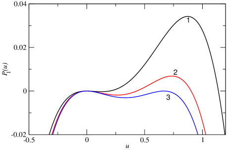
Figure 1: Display of the potential $P_{1}(u)=-\frac{1}{2}\lambda u^{2}+\frac{1}{3}u^{3}-\frac{1}{4}u^{4}$ for Eq. (3) with $\lambda=1/9$, $7/36$ and $2/9$, cases 1-3, respectively. Flatons emerge in the domain between cases 2 and 3. In case 3 wherein $P=P^{\prime}=0$, there are no solitons. Instead kink and/or anti-kink emerge.

Equation (4) yields solitons

$$u=\frac{3\lambda}{1+\sqrt{1-\frac{9\lambda}{2}}\cosh{\left(\sqrt{\lambda}(x-\lambda t)\right)}}$$ (5)

with their peak reaching

$$u_{max}=\frac{2}{3}\Big{(}1-\sqrt{1-\frac{9\lambda}{2}}\Big{)}.$$ (6)

The defocusing effect due to the cubic term enforces an upper bound, $\lambda=2/9$, on the admissible propagation velocities. At the limiting velocity, the soliton (5) flattens into a constant. This is a singular limit for, in addition, also kink and anti-kink emerge,

$$u=\frac{2}{3\left(1+\exp(\mp\frac{\sqrt{2}}{3}s)\right)}~{}~{}~{}{\rm{where}}~{}~{}~{}s=x-\frac{2}{9}t.$$ (7)

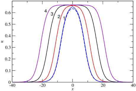
Figure 2: Comparison between the approximate shape (solid lines) of the G(1) flaton, Eq. (8), and the exact solution (dashed lines) for a several values of $x_{0}$ (or $\epsilon$, see Eq. (10)): 1- $x_{0}=8.0$ ($\Rightarrow\epsilon=0.05$), 2- $x_{0}=11.27$ ($\Rightarrow\epsilon=10^{-2}$), 3- $x_{0}=16.13$ ($\Rightarrow\epsilon=10^{-3}$), 4- $x_{0}=21.01$ ($\Rightarrow\epsilon=10^{-4}$). Notably, apart of the first pair with visible difference at the top between the exact solution and its approximation, in other cases, they are truly indistinguishable.

The disconnection between solitons and kinks can be also seen from the underlying potential $P_{1}$ in Fig. 1; as $\lambda\rightarrow 2/9$, potential’s top comes down, but once it touches the u-axis, solitons dissolve and instead a kink and anti-kink emerge.

To unfold the 1D flatons we proceed as follows: first, we join the kink with an anti-kink into a pair, with their centers (defined as the location where $u$ assumes half of its maximal value) placed at $\pm x_{0}$, $x_{0}\gg 1$. Clearly, for a finite $x_{0}$ such structure

$$u=\frac{2}{3\left(1+\exp{\left[\frac{\sqrt{2}}{3}\left(|x|-x_{0}\right)\right]}\right)}~{}~{}~{}-\infty<x<\infty.$$ (8)

is an approximate solution. It will be used as an initial input for Eq. (3).

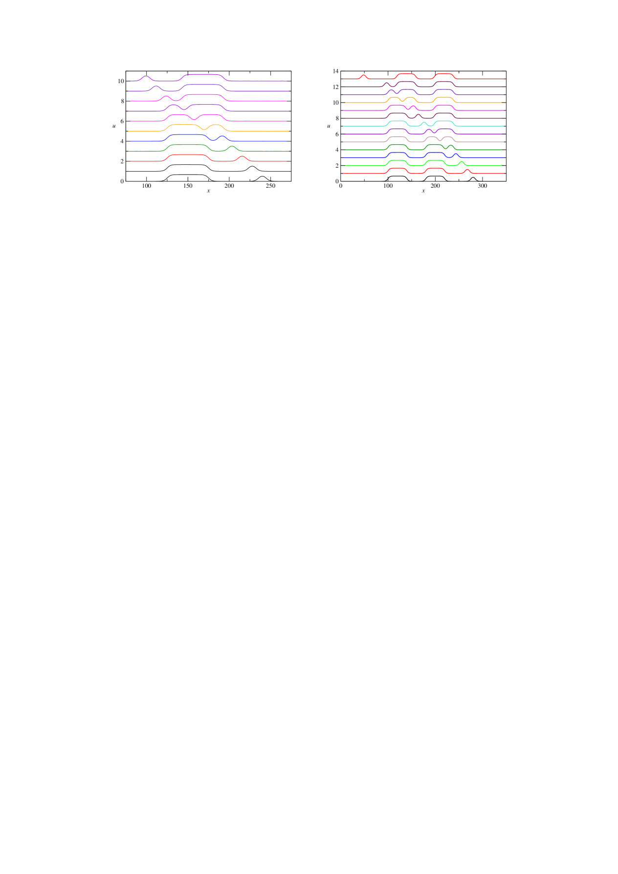
Figure 3: Interaction between G(1) flatons and a soliton. Left panel: Space-time display of the interaction of a wide flaton, $x_{0}=25$, with a $\lambda=0.21$ soliton, shown here and elsewhere in a reference frame moving with the kink velocity of the flaton. From the bottom to the top; the time ranges from $t=0$ to $t=10^{4}$ with time intervals of $1000$. Right panel: Space-time display of the interaction between two equal flatons, $x_{0}=20$, with a $\lambda=0.21$ soliton. From the bottom to the top, the time ranges from $t=0$ to $12000$ with time intervals of $1000$ and finally $t=16000$.

Given by Eq. (8) $u$ is continuous at $x=0$, where $\displaystyle u\simeq 1-\exp{\left(-\frac{\sqrt{2}}{3}x_{0}\right)}$, and though its derivative undergoes a finite jump $[u]\simeq 2\exp{\left(-\frac{\sqrt{2}}{3}x_{0}\right)}$, for $1<<x_{0}$ the jump is very small and decreases very quickly with $x_{0}$. Indeed, as clearly seen in Fig. 2, the approximate solution converges very quickly with $x_{0}$ to the exact solution.

The solutions of the Gardner equation and other partial differential equations considered, are numerically determined using periodic boundary conditions in a sufficiently large domain employing the Newton-Kantorovich procedure Boyd which has second-order accuracy in both time and space and an implementation similar to the one in Dji1995 , for details see RO .

To test the viability and robustness of flatons we let them collide with solitons. As seen in Fig. 3, they reemerge in their original form without any observable debris, with the left panel displaying the interaction between a wide flaton and a relatively fast (and large) soliton ($\lambda=0.21<2/9$), whereas on the right panel, we combine a pair of equal-width flatons and follow their interaction with a soliton. Note that by the time the soliton collides with the flaton, the latter has already settled into its ultimate form.

The soliton-flaton interactions clearly indicate that flatons are more than merely approximate solutions and there should be an underlying analytical structure. Indeed, it was always there, it just had to be unfolded. The ’trick’ is not to take the $\lambda\rightarrow 2/9$ limit but to focus on a narrow layer squeezed between the upper solitons range, Eq. (5), and their barrier where kink/antikink form. Flatons saga can be read from the left panel of Fig. 4 where we draw profiles of $u$; whereas at small velocity $\lambda$, solitons have their usual peaked shape, upon approaching their upper speed limit, their shape changes drastically and rather than to grow with $\lambda$, a slightest increase in velocity causes them to widen very quickly.

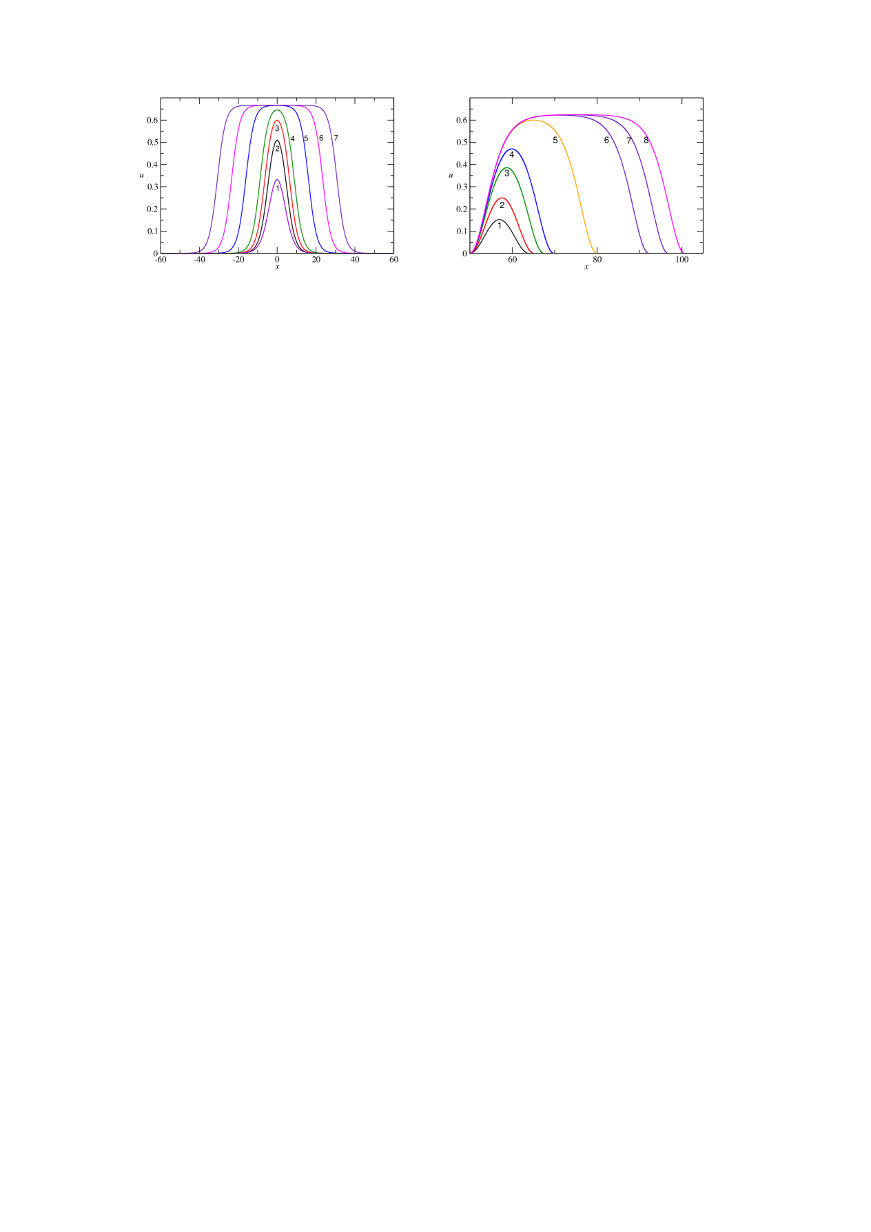
Figure 4: Left panel: Soliton’s profile as an ascending function of its velocity $\lambda=1/6,~{}0.21,~{}0.22,~{}0.222,~{}2(1-10^{-6})/9,~{}2(1-10^{-9})/9$ and $2(1-10^{-12})/9$, respectively. Note the structural change that soliton’s shape undergoes as $\lambda\rightarrow 2/9$; their top flattens, the amplitude hardly changes and they turn into a sequence of ever widening flatons. Right panel: Profiles of G(2) compactons, Eq. (1) with $n=2$, as a function of $\lambda$. When $\lambda\rightarrow 15/64$, compactons turn into flatons. Cases 1 to 8 correspond to $\lambda=0.1,~{}0.15,~{}0.2,~{}0.22,~{}0.234,~{}0.23437,~{}0.234374$, and $0.23437475$, respectively.

To ’extract’ those features from solitons formula (5), we define

$$\lambda_{f}=\frac{2}{9}\Big{(}1-\epsilon^{2}\Big{)}~{}~{}~{}~{}{\rm{where}}~{}~{}0<\epsilon\ll 1,$$

then, in terms of $\epsilon$, Eq. (5) reads

$$u=\frac{2}{3}\left(\frac{1-\epsilon^{2}}{1+\epsilon\cosh{\left[\sqrt{\lambda_{f}}(x-\lambda_{f}t)\right]}}\right)$$ (9)

and thus $u_{max}=\frac{2}{3}(1-\epsilon)$.

Comparing the exact solution with its approximation (8) we find their difference to be ${\cal{O}}\left(\epsilon^{2}\right)$ and the extent of soliton’s profile widening and flattening may be expressed via $x_{1/2}$ where the soliton’s amplitude has decreased by half, i.e., when

$$x_{1/2}\simeq\frac{3}{\sqrt{2}}\ln{\frac{2}{\epsilon}}.$$ (10)

Thus, velocity change $\sim 1-\epsilon^{2}$ and amplitude change $\sim 1-\epsilon$, cause the corresponding flaton to widen as $\sim\ln{1/\epsilon}$.

That 1D flatons went for so long unnoticed may perhaps be due to their very narrow domain of attraction. The left panel of Fig. 5 displays emergence of a flaton out of a carefully orchestrated initial excitation. With one exception we have found this feature to be typical of all studied cases. Therefore, it would have been misleading to start unfolding flatons with the left panel of Fig. 5 which is an end result of numerous numerical experiments and was ’extracted’ after the mere existence of flatons was firmly established.

Compact Flatons. Turning to flatons with a compact support we start with
(i)

The G(n=2) equation.

Without the defocusing cubic term, Eq. (1) reduces to the K(2,2) equation RosHym with the underlying compacton

$$u=\frac{4\lambda}{3}\cos^{2}\left(\frac{s}{4}\right)H(2\pi-|s|)~{}~{}~{}{\rm{where}}~{}~{}s=x-\lambda t$$ (11)

($H(y)$ is the Heaviside function), being its basic solitary mode with a compact support. Though K(2,2) is not integrable in the conventional sense, its interactions are remarkably clean RosHym ; RZ .

To derive the compact solitary waves let $u=u(s)$ where $s=x-\lambda t$ and integrate Eq. (1) with $n=2$ twice to obtain

Figure 5: Evolution of carefully tailored initial excitations. Left panel: G(1). $u_{0}(x)=0.66\cos{(x/16)}H(8\pi-|x|)$ which begets as its main response the G(1) flaton, see Eq. (9); the displayed times are $t=0,400,800,1200$ and $t=1600$. Right panel: G(2). $u_{0}=0.66\cos{(x/16)}H(8\pi-|x|)$ which begets as its main response the G(2) compact flaton. The displayed interactions are at time intervals of $\Delta t=100$.

.

$$u^{2}\Big{(}u^{2}_{s}+P(u;\lambda)\Big{)}=0~{}~{}~{}{\rm{with}}~{}~{}~{}P(u;\lambda)=-\frac{\lambda}{3}u+\frac{1}{4}u^{2}-\frac{1}{5}u^{3}$$ (12)

where $u^{2}$ is kept out of the bracket to stress the singular nature at $u=0$ which induces compactness. In terms of $u=\frac{4\lambda}{3}W^{2}$, we obtain

$$4W^{2}_{s}=1-W^{2}+\gamma W^{4}=\gamma(W^{2}_{-}-W^{2})(W^{2}_{+}-W^{2})$$ (13)

where

$$~{}~{}\gamma=\frac{16}{15}\lambda~{}~{}~{}{\rm{and}}~{}~{}W^{2}_{\pm}=\frac{2}{1\mp\sqrt{1-4\gamma}}~{}~{}.$$

Insofar as $\gamma<1/4$ or $\lambda<15/64$, we obtain compactons. Their profiles displayed in the right panel of Fig. 4 may be expressed via elliptic functions, but were determined numerically solving the first order ode Eq. (13) via evaluation of the primitive of the inverse potential function $P(u;\lambda)$. Note that unlike the K(2,2), the width of G(2) compactons depends on their velocity. When $\gamma=1/4$, $W_{-}=W_{+}$, compactons dissolve and semi-compact kink and anti-kink vanishing at $u=0$ emerge

$$u=\frac{5}{8}\tanh^{2}\left(\frac{\pm s}{4\sqrt{2}}\right)H(\pm s),~{}~{}~{}s=x-\frac{15}{64}t.$$ (14)

The right panel of Fig. 5 illustrates the emergence of a compact flaton out of a carefully tailored initial excitation and, as in G(1) shown in the left panel of Fig. 5, is the end result of numerous numerical experiments. The left panel of Fig. 6 displays interaction of the G(2) compact flaton with a G(2) compacton. The flaton emerges unchanged, but the compacton sheds some of its mass.

(ii) The G(n=3) equation.

For the present case we have an exact solution RO

$$u=\frac{3}{5}\left[1-\sqrt{1-\frac{25\lambda}{6}}\cosh{(\frac{s}{3})}\right]_{+}$$ (15)

representing for $\displaystyle 0<\lambda<6/25$ a compacton. As elsewhere, flatons emerge near the edge of their upper range

$$\lambda_{f}=\lambda_{max}(1-\epsilon^{2})~{}~{}~{}{\rm{where}}~{}~{}\lambda_{max}=\frac{6}{25},$$

yielding

$$u=\frac{3}{5}\left[1-\epsilon\cosh{\left(\frac{x-\lambda_{f}t}{3}\right)}\right]_{+}.$$ (16)

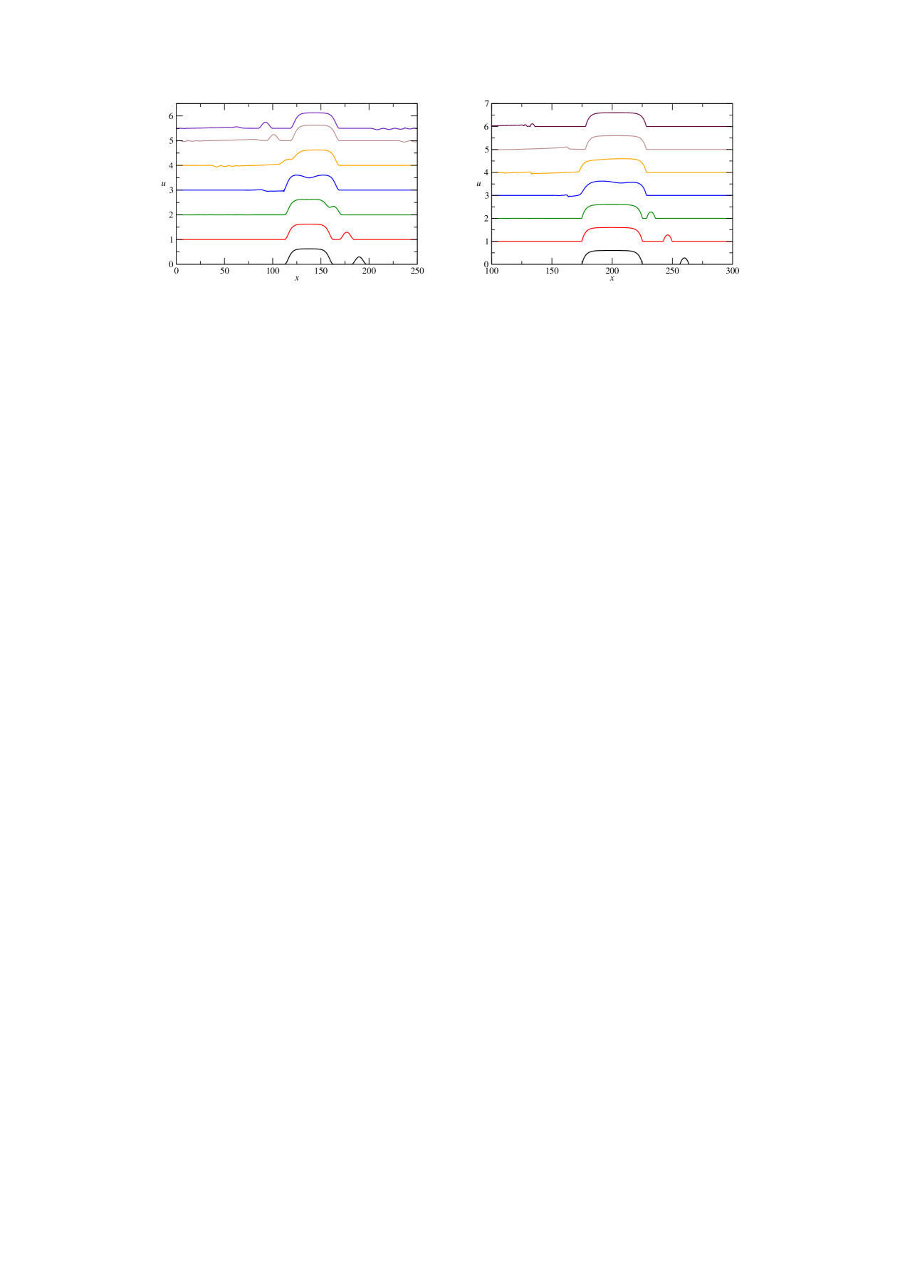
Figure 6: Left panel: G(2)- Interaction of a $\lambda=0.1$ compacton with a $\lambda=0.23437475$ compact flaton. Right panel: G(3)- Interaction of a $\lambda=0.17$ compacton with a $\lambda=0.23999995$ compact flaton. In both cases, flatons reemerge from the encounter unchanged, but in both cases the smaller compacton sheds some of its mass. The snapshots in both panels correspond to time intervals of $200$.

The right panel of Fig. 6 displays G(3) compact flaton colliding with a G(3) compacton. The flaton emerges unaffected, but the compacton loses a big chunk of its mass. We note that unlike all other studied cases, G(3) flatons emerge quite ’naturally’ out of generic initial excitations (not shown). This could be attributed, at least in part, to the fact that since for G(3) flatons $u<0.6$, the convection velocity $C(u)$ remains always positive. We shall further comment on this issue in the last section.

3. Multi-dimensional Flatons

We now turn to the multi-dimensional extension of the Gardner equation (2) and seek spherically symmetric solitary waves $U(r=\sqrt{s^{2}+y^{2}+z^{2}})$, $s=x-\lambda t$, that propagate in x-direction. Hereafter we address only the $n=1$ case. Other cases are deferred to a future publication.

After one integration

$$-\lambda U(r)+{c_{+}U^{\kappa}-c_{-}U^{\ell}+\frac{d-1}{r}U^{\prime}(r)+U^{\prime\prime}}=0,~{}~{}~{}\kappa,\ell>1.$$ (17)

Assuming $r$ to play the role of time, $(d-1)/r$ may be looked upon as a time-dependent ’friction coefficient’ which decays with time. Another formal integration yields

$$\frac{1}{2}U^{\prime 2}+P(U)+(d-1)\int{\frac{dr}{r}{U^{\prime 2}}}=E_{0}~{}~{}~{}$$ (18)

where

$$P(U)=-\frac{\lambda}{2}U^{2}+{c_{+}\frac{U^{1+\kappa}}{1+\kappa}-c_{-}}\frac{U^{1+\ell}}{1+\ell}$$ (19)

with $E_{0}$ playing the role of an effective total energy.

Consider again the potential landscape on Fig. 1. To overcome the ’friction’ present whenever $d>1$, the starting point $u_{0}$ from which the ”particle” starts its descent has to be moved up the potential hill. As in 1D case, if potential’s peak is close enough to the u-axis then the spherical solitary wave will be a flaton, but now things are a bit more involved for if the particle does not have initially a sufficient potential energy, the friction may stop it prior to its arrival to the origin. This difficulty is resolved noting that since on potential’s top the particle can rest indefinitely, thus, being close enough to the top, enables the particle to delay its descent until the time-dependent friction $(d-1)/r$ becomes sufficiently suppressed, so that it could not prevent the particle from arriving to the origin. The longer the particle ’waits’, the longer becomes its flat top.

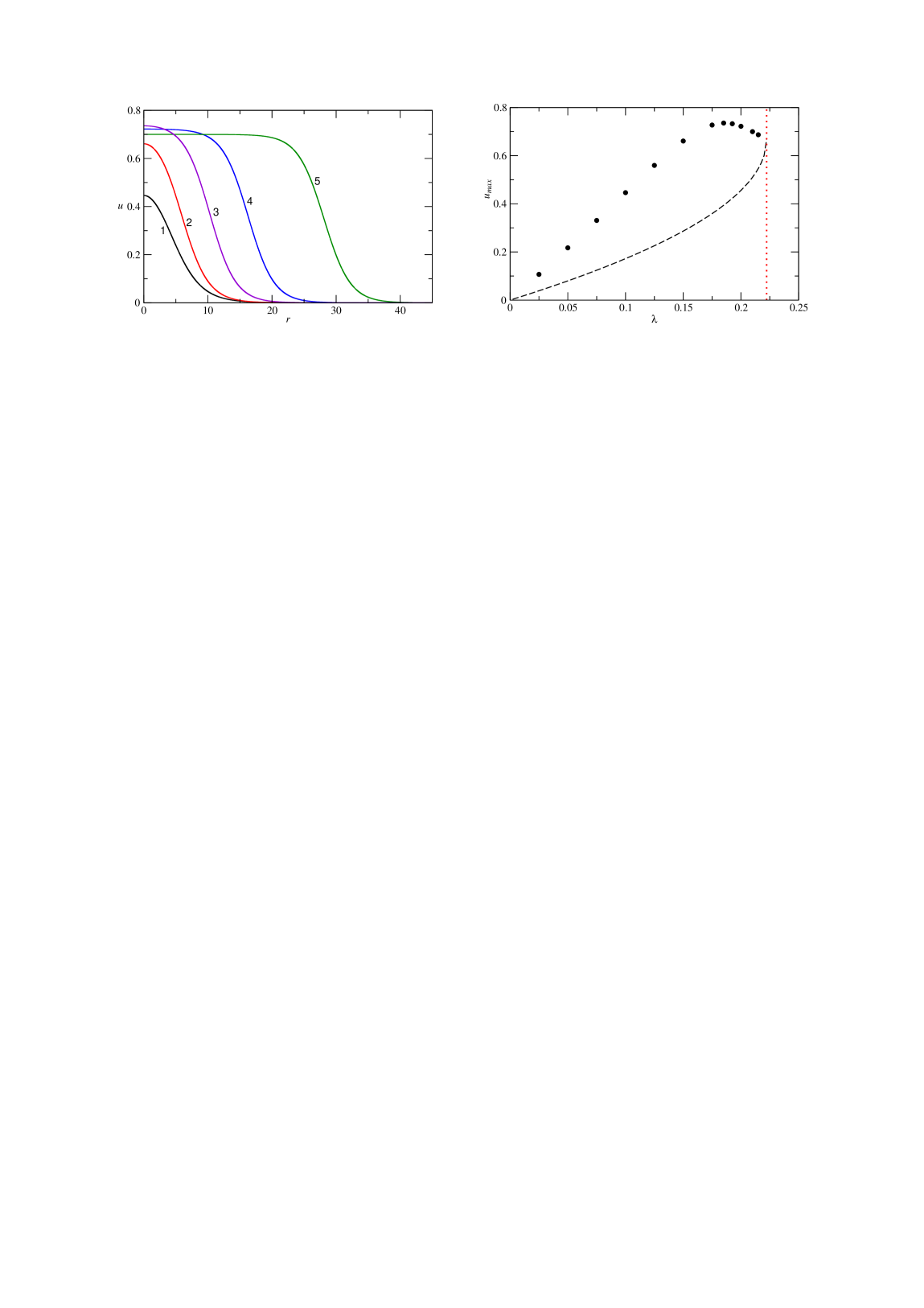
Figure 7: $G_{3}^{1}(2,3)$, Eq. (2). Left panel: Displays 1-5 correspond to $\lambda=0.1,~{}0.15,~{}0.185,~{}0.2$ and $0.21$, respectively, with the latter two being flatons, whereas the corresponding 1D patterns in Fig. 4 are still very much conventional solitons. Note the non-monotone dependence of solitons amplitudes on their speed, explicitly shown by the circles on the right panel, which happens concurrently with the emergence of flatons; for though soliton’s peak ascends with $\lambda$ toward potential’s top, this does not compensate for potential’s descent toward the u-axis. The dashed curve displays the $\lambda$-dependence of the maximal amplitude, $u_{max}$, of the 1D solitons/flatons, see Eq. (6). The vertical dotted line at $\lambda=2/9$ marks the upper limit of the admissible propagation speeds.

Left panel of Fig. 7 is the 3D counterpart of Fig.’s 4 left panel and, as expected, shows that 3D flatons exist for a much wider range of velocities. The right panel of Fig. 7 displays the non-monotone dependence of solitons peak $u_{max}(\lambda)$ on its velocity. Insofar that solitons peak is far from potential’s top then, as in 1D, $u_{max}(\lambda)$ increases with $\lambda$. However, since concurrently with $\lambda$ increase, potential’s top decreases, from a certain velocity on solitons peak comes close enough to potential top so that flatons form. From now on, though with a further increase in velocity, soliton’s peak will be even closer to the top, this will not compensate for potential’s descent toward the $u$-axis, with the net effect that flatons amplitude, as clearly seen in Fig. 7 decreases. As velocity approaches its upper bound, $u_{max}(\lambda)$ approaches from above the amplitude (=2/3) of 1D kinks.

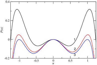
Figure 8: The $G_{1}^{1}(3,5)$ potential, Eq. (21): $P=-\frac{u^{2}}{2}\big{(}\lambda-2u^{2}+u^{4}\big{)}$. Cases 1-3 correspond to $\lambda=0.7$, $0.95$ and $1$, respectively. The second case begets flatons. The third - kinks/antikinks.

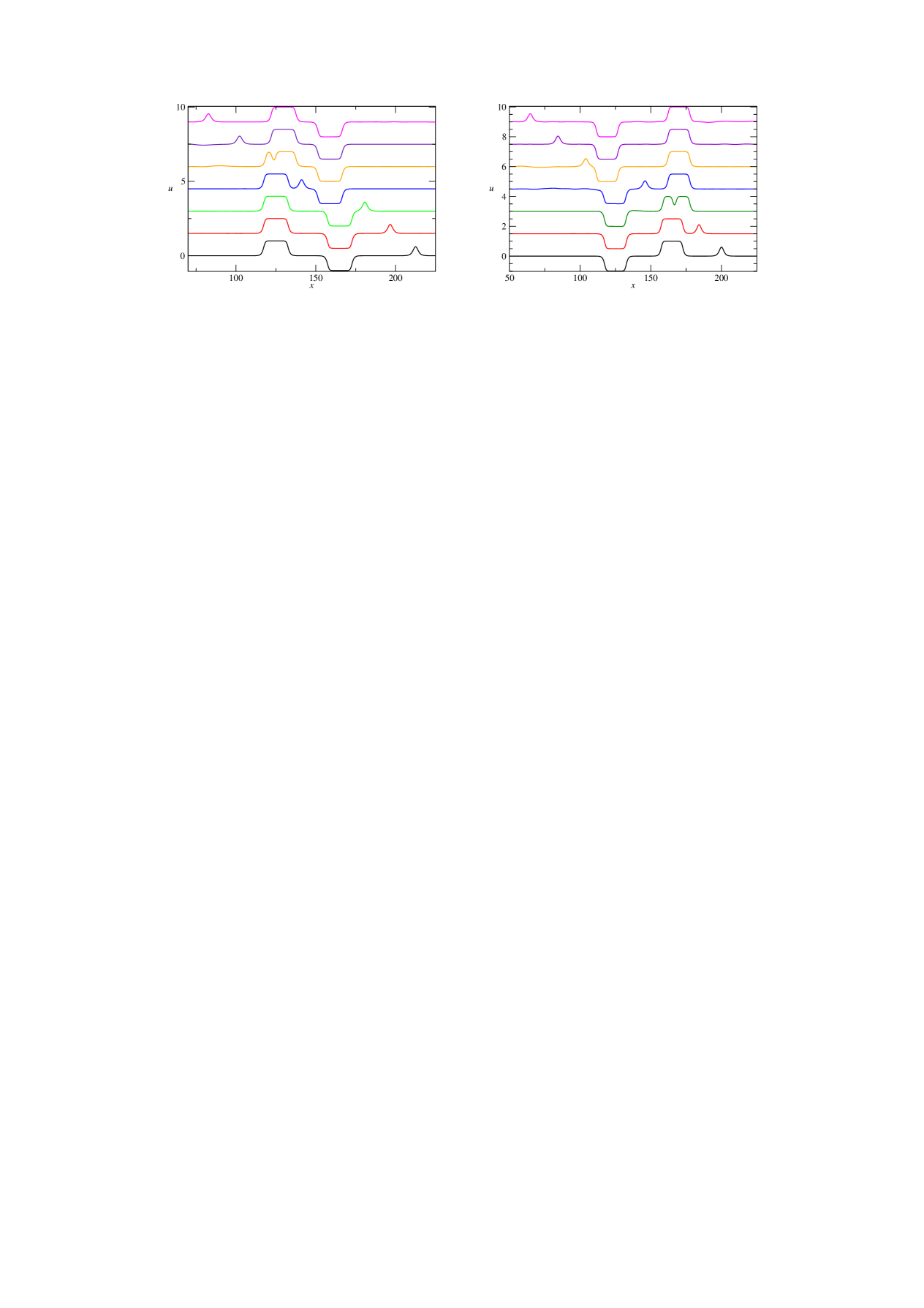
Figure 9: $G_{1}^{1}(3,5)$, Eq. (20). Left panel: Interaction of a $\lambda=0.6$ soliton, Eq. (22), with flaton-antiflaton formation, $\epsilon=10^{-6}$, Eq.(25). Right panel: The antiflaton and the flaton have switched their positions causing an opposite post collision dislocation. Both displays are in a reference frame moving with $\lambda_{f}=1-\epsilon^{2}$. On both panels the shown displays, from the bottom up, are at time intervals of $\Delta t=40$.

The $\mathbf{G_{3}^{1}(3,5)}$. It is convenient to address first its 1D variant

$$G_{1}^{1}(3,5):~{}~{}~{}u_{t}+\left(4u^{3}-3u^{5}\right)_{x}+u_{xxx}=0,$$ (20)

with its underlying traveling waves potential, see Fig. 8,

$$P(u)=-\frac{u^{2}}{2}\big{(}\lambda-2u^{2}+u^{4}\big{)}$$ (21)

which for $0<\lambda<\lambda_{max}=1$ admits solitary solutions

$$u=\pm\frac{\sqrt{\lambda}}{\sqrt{1+\sqrt{1-\lambda}\cosh\left[2\sqrt{\lambda}(x-\lambda t)\right]}},$$ (22)

peaking at

$$u_{max}^{2}=1-\sqrt{1-\lambda},$$ (23)

and kinks when $\lambda=1$

$$u=\pm\frac{1}{\sqrt{1+\exp{\left(2(x-t)\right)}}}.$$ (24)

Let $\lambda_{f}=(1-\epsilon^{2})\lambda_{max}=1-\epsilon^{2}$, $0<\epsilon<<1$, then flatons follow

$$u=\pm\frac{{\sqrt{1-\epsilon^{2}}}}{\sqrt{1+\epsilon\cosh{\left[2\sqrt{1-\epsilon^{2}}(x-\lambda_{f}t)\right]}}}.$$ (25)

Here, the convection velocity $C(u)=12u^{2}-15u^{3}$ reverses its direction and whenever $\sqrt{0.8}<u$, it acts in a direction opposite to flatons motion. Yet, as can be seen in Fig. 9, this does not seem to have a direct impact on their dynamics: both flatons and anti-flatons seem very robust, and their interaction with solitons is fairly clean, though solitons seem to lose some mass. Also, since the collision causes the flaton (anti-flaton) to move to the right (left), the distance between the flaton and anti-flaton decreases when the anti-flaton is hit first, see the left panel, but increases when the flaton is the one to be hit first, see the right panel. However, convection’s reverse of direction within flatons amplitude range manifests itself otherwise; even with a careful tailoring of initial excitations we did not observe flatons emerge. They had to be ’planted’ ab initio.

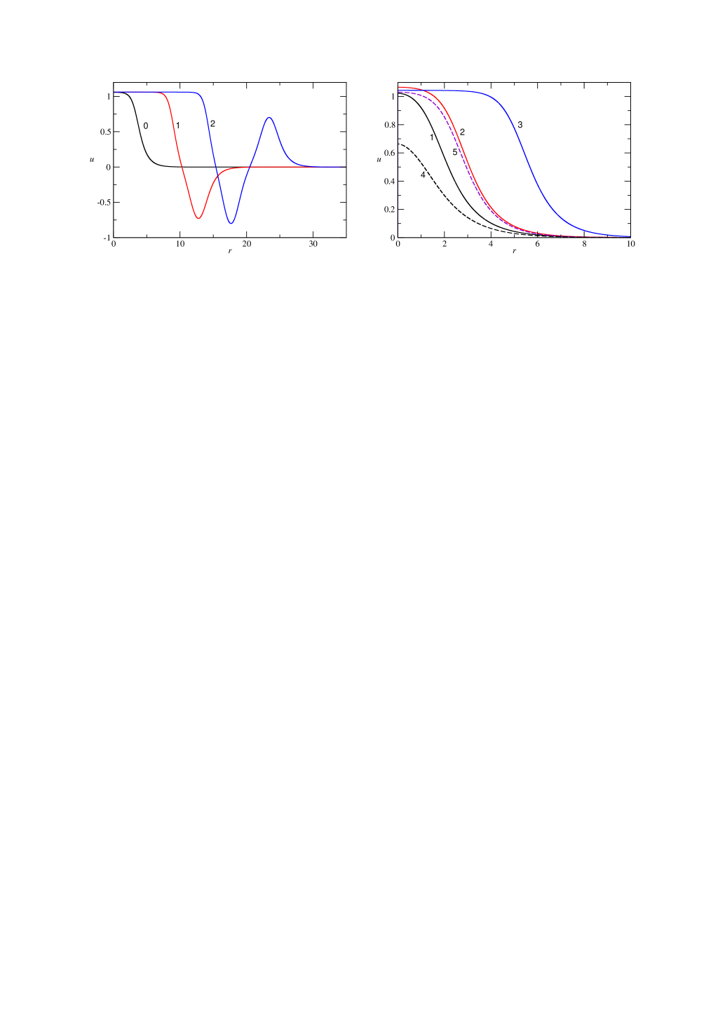
Figure 10: $G_{3}^{1}(3,5)$. Left panel: Display of the first three $\lambda=0.7$ 3D flatons. Right panel: $\lambda=0.4,~{}0.6$ and $0.8$ 3D solitons marked by 1, 2 and 3, respectively and $\lambda=0.8$ solitary waves in one and two dimensions marked by 4 and 5, respectively.

A far richer scenario awaits us in the spherical extension of the problem. Let $u=u_{0}(\lambda)$ be the initial position of a ”particle” on potential’s particular positive branch descending from there to $u=0$. Now, since the potential is symmetric, a further climb on the positive hill will lead to point $u_{1}$ where the descending particle has a sufficient potential energy to overcome the friction, pass through the origin, make one round in the negative well and settle at the origin. A further climb along the potential leads to point $u_{2}$ which equips the ”particle” with adequate potential energy to make two rounds between the two potential wells prior to its settling at the origin.

For an unbounded potential like $P(u)=-u^{2}+u^{4}$, the above procedure would beget an infinite sequence of $N$-nodal solitons, however, since the relevant potential $P(u)$ with $\kappa=2$ and $\ell=4$ peaks at

$$u^{2}_{P_{max}}=\frac{2}{3}\Big{(}1+\sqrt{1-\frac{3\lambda}{4}}\Big{)},~{}~{}\lambda\leq 1,$$ (26)

a climb along potential’s specific branch can proceed only so far. Yet, in this case as well there is a sequence of multi-nodal solitons, but now they condense near the potential’s top. Again, a ”particle” close enough to the top may wait there until ’friction’ becomes sufficiently suppressed and let the particle execute exactly $N$-oscillations prior to its settling at the origin. One thus derives a sequence of modes condensing near potential’s top with $(N+1)$-nodal soliton ”waiting” for a longer ’time’ and thus acquiring a longer quasi-plateau than its $N$-nodal predecessor prior to its descent. The left panel of Fig. 10 displays a $\lambda=0.7$ example of first three such modes. Note that the difference between the initial values of $u_{0}$, $u_{1}$ and $u_{2}$ is smaller than $10^{-8}$. Also, since the 3D ’friction’ is larger than the planar one, the spherical particle has to hover near the top for a longer ’time’ which results in both slightly higher initial amplitude than the respective 2D case, and a longer quasi-plateau, see the right plate of Fig. 10. The latter also shows that with an increase in $\lambda$ solitons transform to flatons emerging already at $\lambda\approx 0.6\lambda_{max}$.

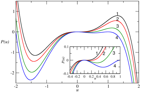
Figure 11: The potential $P=-\frac{\lambda}{2}u^{2}+u^{3}-{\frac{1}{3}}u^{5}$ of Eq. (27) with $\kappa=2$, $\ell=4$, $c_{+}=3$ and $c_{-}=5/3$, for $\lambda=0.2,~{}0.5,~{}1$ and $4/3$ marked by 1 - 4, respectively. The inset: vicinity of the origin.

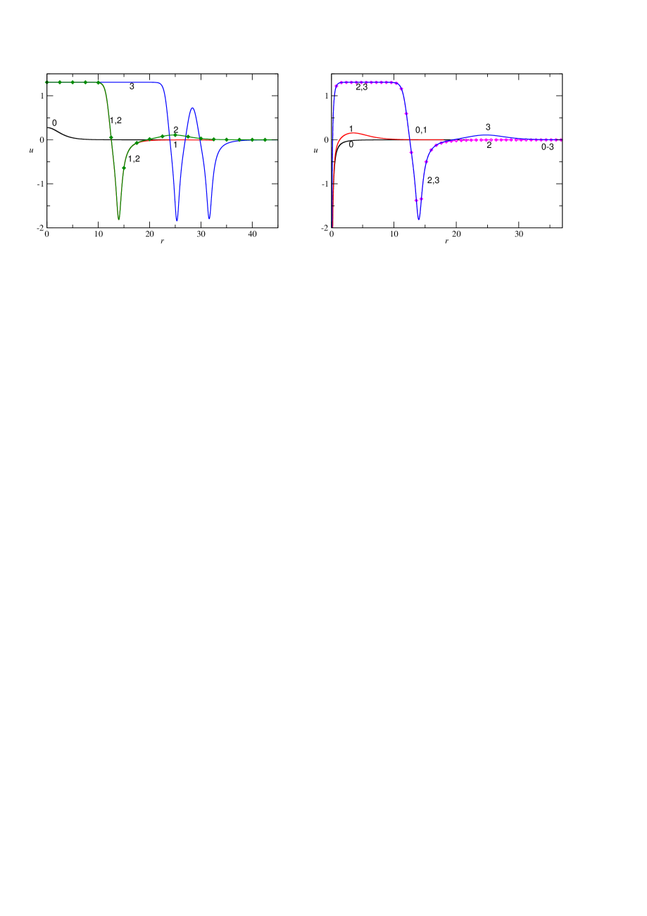
Figure 12: $\lambda=0.2$. Bright and dark spherical solitons of Eq. (27). Left panel: The first four bright modes. Note that up to $r\approx 20$, modes 1 and 2 coincide visually. Right panel: The first four dark modes. Notably, apart of a very narrow layer near dark modes origin where $u_{0}=-6.54976\ldots$, $u_{1}=-7.02246$ …, $u_{2}=-15.821105239848875\ldots$ and $u_{3}=u_{2}-5.21\times 10^{-13}$, bright and dark modes look very similar!

Thus, whereas in 1D, for flatons to emerge we need the potential top to come close enough to the $u$-axis, in higher dimensions there is a joint action: on one hand one has to climb toward potential’s top on the other, the top comes down which results in flatons forming in a much wider velocities range, c.f., the G(1) case, whereas in a symmetric potential it always assures flatons, though not necessarily starting with the basic $N=0$ mode. Hereafter we shall refer to either a soliton or flaton as an $N$-mode if it crosses $u=0$, $N$ times.

The last case to be considered amalgamates the two previous cases. Let $\kappa=2$ and $\ell=4$. Without loss of generality we assume $c_{+}=3$ and $c_{-}=5/3$. Thus

$$G_{3}^{1}(2,4):~{}~{}~{}u_{t}+\left(3u^{2}-\frac{5}{3}u^{4}\right)_{x}+(\nabla^{2}u)_{x}=0.$$ (27)

The underlying potential of its travelling waves, see Fig. 11,

$$P(u)=-\frac{\lambda}{2}u^{2}+u^{3}-{\frac{1}{3}}u^{5},$$ (28)

has two very asymmetric wells. Its positively valued branch admits the so-called bright solitons, i.e., solitons which assume a positive value at the origin, in a bounded velocity range, whereas the negative branch, $u<0$, supports dark ones, i.e., solitons which assume a negative value at the origin, for any $\lambda$. In more detail:

1) Bright modes. Since potential’s negative branch reflects all particles coming from the positive side, they may then condense near potential’s top. Left panel of Fig. 12 displays an example of the first four spherical modes from the basic $N=0$ till $N=3$.

2) Dark modes: Let $u=u_{0}<0$ denote the amplitude of its 0-nodal dark soliton. Now let $u=u_{top}$ be a point on the negative branch such that a ”particle” released from $P(u_{top})$ lands on the top of potential’s positive branch. Clearly, any initial position $u<u_{top}$ will cross potential’s top and roll to infinity. Thus, the dark modes range is limited to the $u_{top}<u<u_{0}<0$ strip. One may now attempt to repeat the condensation scenario of the previous case near the positive top by launching particles sufficiently close to $u=u_{top}$, expecting them to land near the top and wait there until the ’friction’ is subdued and then repeat the spiel: descend to the valley and execute $N$ oscillations prior to settling at the origin. Such solution would start as a dark entity followed by a flat part and conclude with an oscillatory tail, c.f., right plate of Fig. 12 where four such modes are displayed.

Finally, we pause to note that all multi-dimensional solutions presented in this section were numerically found solving Eq. (17) amended with boundary conditions $U^{\prime}(r=0)=0$, and $U(r\to\infty)\to 0$ for the relevant values of $\kappa$, $\ell$ and $c_{\pm}$ via a shooting method based on fourth-order Runge- Kutta scheme with a typical $\Delta r=O\left(10^{-5}\right)$ step size. In spite of using quadruple-precision, 128 bit computations, we were unable to unfold numerically more than three sign-changing modes, with the difficulty escalating very quickly as $\lambda$ increases toward the limiting value beyond which the solution diverges. To appreciate the computational difficulty, note that the convergence to the far-field condition $r\to\infty$ requires exceedingly small changes in $u(r=0)$, for instance at the $17^{th}$ digit in the case of the $0^{th}$-mode for $\lambda=0.215$ shown in the right panel of Fig. 7. Part of the difficulty stems from the fact that unlike the previous cases which were initiated from the positive top’s vicinity, and we were able to control their starting point, and thus the waiting time, with the starting point located on the negative branch, we have no direct control over the landing point on the positive branch, and apart of the first four cases, searching for higher modes we always either ended in the negative well or escaped all together the potential hill. Though one cannot preclude that higher $N$ modes could be unfolded with a much higher precision, a truly-high $N$ modes seem to be out of reach for both dark and bright modes.

4. Summary

The present work focuses on unfolding flatons - flat-top - solitons which emerge in dispersive systems whenever solitons range is bounded from above. Whereas in two or three dimensions any solution hovering long enough close to potential’s peak, or better yet. emerging there, may be ’colonized’ by a flaton(s), for 1D flatons to emerge, potential’s peak has to be brought down sufficiently close to the u-axis, which takes place only when solitons speed approaches the top of its range. This makes 1D flatons far more delicate affair; they are very sensitive to even a minute change of their velocity which causes a dramatic change of their width.

Finally, we comment upon 1D flatons domain of attraction which with one exception is very narrow, as one can witness from the carefully orchestrated initial excitations in Fig. 5 which beget flatons and were done posteriori after flatons existence was already established. Though, as we have stressed, the existence of flatons bears no consequence as to their robustness once they emerge or are planted ab initio. Two cases are to be contrasted: whereas for $G_{1}^{1}(3,5)$ we were unable to see flatons emerging from any reasonable initial conditions, for G(3) they emerge quite naturally from any generic initial excitation. The only plausible explanation that comes to mind is that whereas G(3) flatons amplitude evolves within cooperative domain of convection, in the $G_{1}^{1}(3,5)$ case flatons amplitude, $0\leq u<1$, falls within a regime where convection reverses its direction, $C(u=\sqrt{0.8})=0$, and opposes in part motion of the flaton. G(1) is a borderline case: convection vanishes at $u=2/3$ which is flatons’ upper bound, whereas G(2) represents an intermediate case between G(1) and G(3). This perhaps answers in part why unlike the spherical flatons which were already noted before in the complex field theory Q-balls ; Q-balls2 , 1D flatons have hitherto escaped our attention. In closing, we note that flatons in spatially discrete system will be addressed in RoPi .

Declaration of Competing Interest

The authors declare that they have no known competing financial interests or personal relationships that could have appeared to influence the work reported in this paper.

Figures captions

Fig.1: Display of the potential $P_{1}(u)=-\frac{1}{2}\lambda u^{2}+\frac{1}{3}u^{3}-\frac{1}{4}u^{4}$ for Eq. (3) with $\lambda=1/9$, $7/36$ and $2/9$, cases 1-3, respectively. Flatons emerge in the domain between cases 2 and 3. In case 3 wherein $P=P^{\prime}=0$, there are no solitons. Instead kink and/or anti-kink emerge.

Fig. 2: Comparison between the approximate shape (solid lines) of the G(1) flaton, Eq. (8), and the exact solution (dashed lines) for a several values of $x_{0}$ (or $\epsilon$, see Eq. (10)): 1- $x_{0}=8.0$ ($\Rightarrow\epsilon=0.05$), 2- $x_{0}=11.27$ ($\Rightarrow\epsilon=10^{-2}$), 3- $x_{0}=16.13$ ($\Rightarrow\epsilon=10^{-3}$), 4- $x_{0}=21.01$ ($\Rightarrow\epsilon=10^{-4}$). Notably, apart of the first pair with visible difference at the top between the exact solution and its approximation, in other cases, they are truly indistinguishable.

Fig. 3: Interaction between G(1) flatons and a soliton. Left panel: Space-time display of the interaction of a wide flaton, $x_{0}=25$, with a $\lambda=0.21$ soliton, shown here and elsewhere in a reference frame moving with the kink velocity of the flaton. From the bottom to the top; the time ranges from $t=0$ to $t=10^{4}$ with time intervals of $1000$. Right panel: Space-time display of the interaction between two equal flatons, $x_{0}=20$, with a $\lambda=0.21$ soliton. From the bottom to the top, the time ranges from $t=0$ to $12000$ with time intervals of $1000$ and finally $t=16000$.

Fig. 4: Left panel: Soliton’s profile as an ascending function of its velocity $\lambda=1/6,~{}0.21,~{}0.22,~{}0.222,~{}2(1-10^{-6})/9,~{}2(1-10^{-9})/9$ and $2(1-10^{-12})/9$, respectively. Note the structural change that soliton’s shape undergoes as $\lambda\rightarrow 2/9$; their top flattens, the amplitude hardly changes and they turn into a sequence of ever widening flatons. Right panel: Profiles of G(2) compactons, Eq. (1) with $n=2$, as a function of $\lambda$. When $\lambda\rightarrow 15/64$, compactons turn into flatons. Cases 1 to 8 correspond to $\lambda=0.1,~{}0.15,~{}0.2,~{}0.22,~{}0.234,~{}0.23437,~{}0.234374$, and $0.23437475$, respectively.

Fig. 5: Evolution of carefully tailored initial excitations. Left panel: G(1). $u_{0}(x)=0.66\cos{(x/16)}H(8\pi-|x|)$ which begets as its main response the G(1) flaton, see Eq. (9); the displayed times are $t=0,400,800,1200$ and $t=1600$. Right panel: G(2). $u_{0}=0.66\cos{(x/16)}H(8\pi-|x|)$ which begets as its main response the G(2) compact flaton. The displayed interactions are at time intervals of $\Delta t=100$.

Fig. 6: Left panel: G(2)- Interaction of a $\lambda=0.1$ compacton with a $\lambda=0.23437475$ compact flaton. Right panel: G(3)- Interaction of a $\lambda=0.17$ compacton with a $\lambda=0.23999995$ compact flaton. In both cases, flatons reemerge from the encounter unchanged, but in both cases the smaller compacton sheds some of its mass. The snapshots in both panels correspond to time intervals of $200$.

Fig. 7: $G_{3}^{1}(2,3)$, Eq. (2). Left panel: Displays 1-5 correspond to $\lambda=0.1,~{}0.15,~{}0.185,~{}0.2$ and $0.21$, respectively, with the latter two being flatons, whereas the corresponding 1D patterns in Fig. 4 are still very much conventional solitons. Note the non-monotone dependence of solitons amplitudes on their speed, explicitly shown by the circles on the right panel, which happens concurrently with the emergence of flatons; for though soliton’s peak ascends with $\lambda$ toward potential’s top, this does not compensate for potential’s descent toward the u-axis. The dashed curve displays the $\lambda$-dependence of the maximal amplitude, $u_{max}$, of the 1D solitons/flatons, see Eq. (6). The vertical dotted line at $\lambda=2/9$ marks the upper limit of the admissible propagation speeds.

Fig. 8: The $G_{1}^{1}(3,5)$ potential, Eq. (21): $P=-\frac{u^{2}}{2}\big{(}\lambda-2u^{2}+u^{4}\big{)}$. Cases 1-3 correspond to $\lambda=0.7$, $0.95$ and $1$, respectively. The second case begets flatons. The third - kinks/antikinks.

Fig. 9: $G_{1}^{1}(3,5)$, Eq. (20). Left panel: Interaction of a $\lambda=0.6$ soliton, Eq. (22), with flaton-antiflaton formation, $\epsilon=10^{-6}$, Eq.(25). Right panel: The antiflaton and the flaton have switched their positions causing an opposite post collision dislocation. Both displays are in a reference frame moving with $\lambda_{f}=1-\epsilon^{2}$. On both panels the shown displays, from the bottom up, are at time intervals of $\Delta t=40$.

Fig. 10: $G_{3}^{1}(3,5)$. Left panel: Display of the first three $\lambda=0.7$ 3D flatons. Right panel: $\lambda=0.4,~{}0.6$ and $0.8$ 3D solitons marked by 1, 2 and 3, respectively and $\lambda=0.8$ solitary waves in one and two dimensions marked by 4 and 5, respectively.

Fig. 11: The potential $P=-\frac{\lambda}{2}u^{2}+u^{3}-{\frac{1}{3}}u^{5}$ of Eq. (27) with $\kappa=2$, $\ell=4$, $c_{+}=3$ and $c_{-}=5/3$, for $\lambda=0.2,~{}0.5,~{}1$ and $4/3$ marked by 1 - 4, respectively. The inset: vicinity of the origin.

Fig. 12: $\lambda=0.2$. Bright and dark spherical solitons of Eq. (27). Left panel: The first four bright modes. Note that up to $r\approx 20$, modes 1 and 2 coincide visually. Right panel: The first four dark modes. Notably, apart of a very narrow layer near dark modes origin where $u_{0}=-6.54976\ldots$, $u_{1}=-7.02246$ …, $u_{2}=-15.821105239848875\ldots$ and $u_{3}=u_{2}-5.21\times 10^{-13}$, bright and dark modes look very similar!

References

- (1) Drazin PG, Johnson RS, Solitons, Cambridge University Press; 1989.
- (2) Miura RM, Gardner CS, Kruskal MD, Korteweg-de Vries equation and generalizations, II. existence of conservation laws and constants of motion, J. Math. Phys. 1968, 9:1204 (1968).
- (3) Rosenau P, Hyman JM, Compactons: solitons with finite wavelength”, Phys. Rev. Letts 1993, 70: 564; Rosenau P, What is compacton?, Notices Am. Soc. 2005, 52: 738.
- (4) Rosenau P, Zilburg A, Compactons, J. Phys. A: Math. Theor. 2018, 51: 343001.
- (5) Haskett RP, Witelski TP, Sur J, Localized Marangoni forcing in driven thin films, Physica D 2005, 209: 117.
- (6) Battye RA, Sutcliffe PM, Q-ball dynamics, Nucl. Phys. B 2000, 590: 390; Volkov MS, Wohnert E, Spinning Q-balls, Phys. Rev. D 2002, 66: 085003.
- (7) Rosenau P, Kazdan E, Emergence of compact structures in a Klein-Gordon model, Phys. Rev. Letts. 2010, 104: 034101.
- (8) Boyd JP, Chebyshev and Fourier Spectral Methods, New York: Springer-Verlag; 1989.
- (9) Djidjeli K, Price WG, Twizell EH, Wang Y, Numerical methods for the solution of the third-and fifth-order dispersive Korteweg-de Vries equations, J. Comp. Appl. Math. 1995, 58: 307.
- (10) Rosenau P, Oron A, On compactons induced by a non-convex convection, Commun. Nonlin. Sci. Numer. Simulat. 2014, 19: 1329.
- (11) Rosenau P, Pikovsky A, to be published.