Intent Classification in Question-Answering Using LSTM Architectures

Abstract

Question-answering (QA) is certainly the best known and probably also one of the most complex problem within Natural Language Processing (NLP) and artificial intelligence (AI). Since the complete solution to the problem of finding a generic answer still seems far away, the wisest thing to do is to break down the problem by solving single simpler parts. Assuming a modular approach to the problem, we confine our research to intent classification for an answer, given a question. Through the use of an LSTM network, we show how this type of classification can be approached effectively and efficiently, and how it can be properly used within a basic prototype responder.

1 Introduction

Despite the remarkable results obtained in the different areas of Natural Language Processing, the solution to the Question-Answering problem, in its general sense, still seems far away [1]. This lies in the fact that the search for an answer to a specific question requires many different phases, each of which representative of a separate problem. For this reason, in this work, we have approached the problem confining our attention to the classification of the intent of a response, given a specific question. In other words, our objective is not to classify the incoming questions according to their meaning, but rather referring them to the type of response they may require.

The interest in this case study is not limited to the achievement of the aforementioned objective, but also to the building of a processing block that could be inserted in a larger architecture of an autonomous responder. Furthermore, current chatbot-based dialogue interfaces can also already take advantage of these type of structures [2], [3].

By acting just as an aid in the separation of intents, it is possible to assess incoming questions in a more targeted manner. The objective is to conceive simple systems, such as those based on AIML (Artificial Intelligence Markup Language), to circumvent the extremely complex problem of evaluating all possible variations of the input.

In the following, after an introduction to the LSTM and its main features, the predictive model is presented in two successive steps. Finally, we report an example of a network trained to respond after it has been trained on previous dialogues.

2 A particular RNN: The LSTM

The understanding of natural language is directly linked to human thought, and as such is persistent. During reading, the comprehension of a text does not happen simply through single word understanding, but mostly through the way in which they are arranged. In other words, there is the need to model the dynamics with which individual words arise.

Unfortunately, traditional feedforward neural networks are not directly fit to extrapolate information from the temporal order in which the inputs occur, as they are limited to considering only the current input for their processing. The idea of considering blocks of input words as independent from each other is too limited within the NLP context. Indeed, just as the process of reading for a human being does not lead to a memorization of all the words of the text, but to the extraction of the fundamental concepts expressed, we need a “memory” that is not limited only to explicit consideration of the previous inputs, but compresses all the relevant information acquired at each step into state variables.

This has naturally led to the so-called Recurrent Neural Networks (RNN) [4] that, by introducing the concept of “internal state” (obtained on the basis of the previous entries), have already shown great promise, especially in NLP tasks. The RNNs contain loops inside them, which allow the previous information to pass through the various steps of the analysis. An explicit view of the recurrent system can be obtained by unrolling the network activations considering the individual subnets as copies (updated at each step) of the same network, linked together to form a chain in which each one sends a message to his successor.

In theory, RNNs should be able to retain in their states the information that the learning algorithm finds in a training sequence. Unfortunately, in the propagation of the gradient backwards through time, the effect of desired output values that contribute to the cost function can become so small that, after only a few steps, there is no longer sufficient contribution to parameter learning (vanishing gradient problem). This problem, explored by [5], means that the RNNs can only retain a short-term memory, because the parts of the sequence further away in time is gradually less important. This makes the RNNs useful only for very short sequences.

(a) RNN

(b) LSTM

Figure 1: Schematic representation of a classic RNN and an LSTM network

To overcome (at least in part) the problem of short-term memory, the Long short-term memory (LSTM) [6] architectures were introduced. Unlike a classic RNN network (Figure 1.a), the LSTM has a much more complex single-cell structure (Figure 1.b), in which a single neural network is replaced by four that interact with each other. However, the distinctive element of LSTM is the cell state $c$, which allows information to flow along the chain through simple linear operations. The addition or removal of information from the state is regulated by three structures, called “gates”, each one with specific objectives.

The first, called “forget gate,” has the purpose of deciding the information that must be eliminated from the state. To reach this goal, the state is pointwise multiplied with:

$$f_{t}=\sigma(W_{f}\cdot[h_{t-1},x_{t}]+b_{f}),$$ (1)

that is obtained from a linear (actually affine because of the biases) block that combines the joint vector of the input with the previous output ($[h_{t-1},x_{t}]$), followed by a standard logistic sigmoidal activation function ($\sigma(x)={1\over 1+e^{-x}}$). The forget gate makes possible to delete (values close to zero), or to maintain (values close to one), individual state vector components.

The second gate, called “input gate”, has instead the purpose of conditioning the addition of new information to the state. This operation is obtained through pointwise multiplication between two vectors:

$$i_{t} = \sigma(W_{i}\cdot[h_{t-1},x_{t}]+b_{i}),$$ (2)

$$\tilde{c}_{t} = \tanh(W_{c}\cdot[h_{t-1},x_{t}]+b_{c})$$ (3)

the first (always obtained through a sigmoid activation) which decides the values to update, and the second (obtained through a layer with $tanh$ activation) whose purpose is to create new candidates. Observe that the function $tanh$ has also the purpose of regulating the flow of information, forcing the activations to remain in the interval $[-1;1]$.

Note that the cell status update depends only on the two gates just defined, and is in fact represented by the following equation:

$$c_{t}=f_{t}*c_{t-1}+i_{t}*\tilde{c}_{t},$$ (4)

Finally, there is the “output gate”, that controls the generation of the new output $h_{t}$ for this cell in relation to the current input and previous visible state:

$$o_{t} = \sigma(W_{o}\cdot[h_{t-1},x_{t}]+b_{o}),$$ (5)

$$h_{t} = o_{t}*tanh(c_{t}).$$ (6)

Also, in this case there is a sigmoid activation layer that determines which part of the state to send out, multiplying them by values between zero and one. Note that, again to limit output values, the $tanh$ function is applied to each element of the state vector (this is a simple function without any neural layer) before it is multiplied by the vector determined by the gate.

3 Implementation

Through the recurrent neural networks, with LSTM type architecture, the models used to achieve the intended objective are analysed and described below. Despite the relative simplicity of these architectures (from a general point of view in the dynamic text processing), they prove extremely efficient in being able to catalogue the intent of the answer; demonstrating how the decomposition of the general complex problem can also be tackled simply in its individual parts.

3.1 Embedding

Obviously, and regardless of the type of neural network used, having to deal with text in natural language it is essential to define the type of embedding used. In fact, unlike formal languages, which are completely specified, natural language emerges from the simple need for communication, and is therefore the bearer of a large number of ambiguities. To be able to at least try to understand it, it is therefore necessary to specify a sort of “semantic closeness” between the various terms, transforming the single words into vectors with real values within an appropriate space [7]. The resulting embedding is therefore able to map the single words into a numerical representation that “preserves their meaning”, making it, in a certain sense, “understandable” even to the computer.

Nowadays there are various ways to obtain this semantic space, generally known as Word Embeddings techniques, each with its own peculiarities. For the prefixed purpose it was decided to use a pre-trained embedding known as GloVe [8], based on a vocabulary of 400,000 words mapped in a 300-dimensional space.

3.2 Dataset

A heterogeneous dataset, consisting of questions both manually constructed and published by TREC and USC [9], was used to train and test the various models. This dataset contains 5500 questions in English in the training set and another 500 in the test set. Each question has a label that classifies the answer in a two-level hierarchy. The highest level contains six main classes (abbreviation, entity, description, human, location, numeric), each of which is in turn specialized in distinct subclasses, which together represent the second level of the hierarchy (e.g. human/group, human/ind, location/city, location/country, etc). In total, from the combination of all the categories and the sub-categories we get 50 different labels with which the answer to the supplied question is classified. An example extracted from the dataset is the following (label is marked with bold and the question in italics):

HUMAN:ind  Who was the 16th President of the United States?

As you can see, the label is composed of two parts separated by the symbol ‘:’, representing the main class and the sub class respectively. In this example, the main class indicates that the answer must communicate a person or a group, while the sub class informs that we want to identify a specific individual (obviously through his name).

It should be noted that the representation provided by GloVe covers the totality of the words (9123 words) present in the Dataset, without therefore the need for further work in this sense. However, once the data has been extracted from the dataset, a first manipulation is carried out, which consists in cleaning the strings from any special characters and punctuation symbols (excluding the question mark). Moreover, all the words contained in the strings are transformed into lowercase, thus avoid multiple codings for the same word.

3.3 Models analysis and results

The search for the problem solution has been divided in two steps. It was in fact preferred to create a basic model first, which aimed to classify only the main class, and then continue with a second model that also used the secondary class.

3.3.1 First model

To achieve the first objective, the strategy pursued was to map the entire sequence, entering the network, into a vector of fixed dimensions, equal to the number of main categories. In other words, the procedure foresees that every single word constituting the question (according to the temporal order and after having been mapped through the level of embedding) is placed in input to the LSTM, whose final state is mapped through a classical neural network with Softmax activation in one of the six main prediction classes (Figure 2).

The Table 1 shows the results of the accuracy obtained, both on the training set and on the test set, varying the size of the $h$ state of the LSTM.

Figure 2: Representation of the first classification model

The supervised learning of the model was carried out using the Backpropagation through time (BPTT) [10] algorithm with the classical Categorical Cross-Entropy cost function:

$$L(t,p)=-\sum_{n}\sum_{j}t_{n,j}log(p_{n,j})$$ (7)

where the first summation is extended on the number of evaluated samples (examples) while the second on the number of classes owned; $t_{n,j}$ is the target of the example $n$ represented as one-hot vector where only the $j$-th entry is $1$ and $p_{n,j}$ is the predicted probability that example $n$ belong to class $j$.

h Dimension	Training set	Test set
25	99,26%	87,80%
50	99,94%	89,80%
75	99,94%	90,60%
100	99,98%	90,20%

Table 1: Accuracy relative to the size of the state for the first model

3.3.2 Second model.

The good results obtained in the prediction of the main class, have further encouraged the progress in the development of the model, maintaining the first part unchanged. In this second part we have included the subclass prediction, that having to represent a specialization of the main classes, it must be influenced in some way by the prediction of the first.

The basic idea was therefore simply to add a further element to the end of the question. This added padding element does not carry any kind of information, but it is necessary only to evaluate the output following the one corresponding to the last element of the question. The second last exit, linked to the last element of the question, can be considered just like in the previous case, while the latter depends only on the previous state (represented both by $h_{t-1}$ and $c_{t-1}$) since the embedding representative of the padding element is previously set to a vector of all zeros and hence doesn’t contribute to computation of $h_{t}$ (look at Section 2).

By training the network, in a supervised manner, to associate the sub-category to this output, a dependence will therefore be created on both the main classification and the question itself. The two information coming out of the recursive part are subsequently discriminated by two distinct fully-connected layers with Softmax, thus mapping the input sequence into two fixed size vectors representing the main class and the associated sub class. The schematic representation of the second model just described can be observed in Figure 3.

Figure 3: Representation of the double classification model

The BPTT algorithm is still used for the training phase of the model, but with a subtle difference compared to the previous case: in fact, there will not be a single (Categorical Cross-Entropy) cost function but two, since our goals have doubled.

Table 2 shows the results obtained, with an accuracy of around $80\%$ for the prediction of the sub-category of the samples belonging to the test set. Furthermore, as was to be expected, there are almost identical performances on the main category prediction.

	Training set		Test set
h Dimension	Main class	Sub class	Main class	Sub class
25	99,24%	96,86%	86,20%	74,40%
50	99,94%	99,83%	90,00%	80,00%
75	99,94%	99,72%	91,00%	78,60%
100	99,82%	99,67%	91,20%	82,20%

Table 2: Accuracy relative to the size of the state for the second model

It should be noted that, despite the excellent performance of the model on the training set, it does not seem to have gone into overfitting. This affirmation can be confirmed by observing through the accuracy trend for the model with $H=100$ (Figure 4) both on the training and on the test set at different epochs, which shows how the greater accuracy on the training set does not become pejorative for the test set. In fact, both trends seem to stabilize around a regime value, with slight fluctuations that do not seem to affect the generalization characteristics of the network.

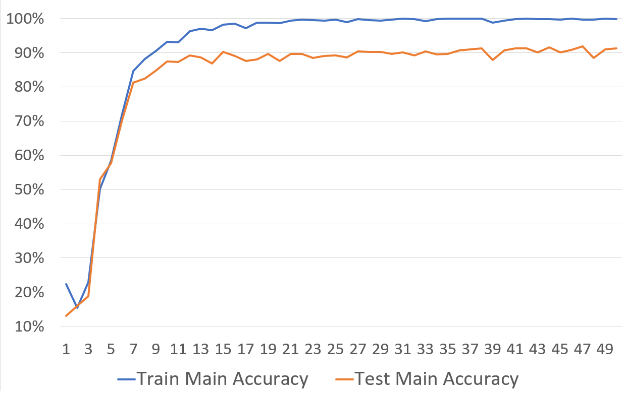
(a)

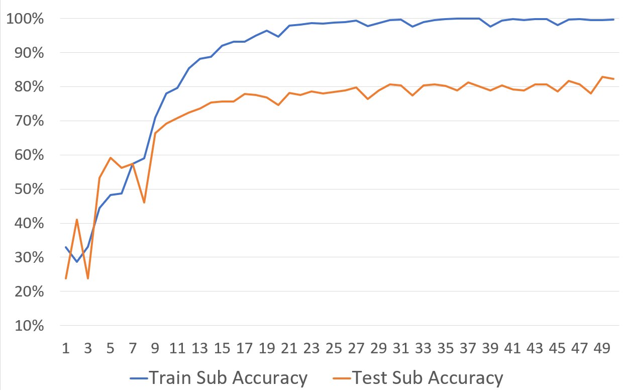
(b)

Figure 4: Accuracy trend for the Main (a) and Sub (b) classes at different epochs.

3.4 Prototype responder

Finally, in order to test (at least briefly) the importance of what was achieved in the classification of intents on the ultimate purpose of creating a responder, it was decided to create a prototype that could exploit the categorization obtained to generate a response. This prototype (Figure 5) uses a bidirectional LSTM (BLSTM) network [11] to review the inbound application, so that it can generate an answer only after acquiring the entire question.

Figure 5: Representation of the responder prototype

The status of this BLSTM network is conditioned by the prediction returned by the previous model. The two vectors representing the main and the sub class are in fact linked together, forming a single vector that will represent the initial state of the BLSTM network. The exits of the network, which constitute the words forming the answer, are thus generated by the analysis of both contexts (future and past), and strongly influenced by the categorization provided.

Question	Answer
How many people speak French?	13
What day is today?	the first day may nights and the
Who will win the war?	north
Who is Italian first minister?	francisco vasquez
When World War II ended?	march
When Gandhi was assassinated?	1976

Table 3: Examples of answers for questions not belonging to the training set

The supervised training of the network was performed on a set of 500 question-answer samples, and in the Table 3 are shown some of the network outputs relating to questions not present in the training set. It should be noted that the purpose of this prototype is not to provide a correct answer (which is quite impossible given the limited dataset and since no knowledge of the answer not relating to it is never provided to the network) but to show how the simple excellent categorization of the intent allows, already alone, to get consistent answers to the context of the question.

4 Conclusion

The results obtained from the models presented show very high accuracy values, both for the training set and for the test set. Networks of this type are actually very effective in this type of classification, perhaps because of their simplicity. The example of the responder prototype then confirms how the choice to classify the questions based on the intent of the answer is extremely effective in limiting and contextualizing the outgoing answer. Consequently, this approach can be of help for the development of more complex systems, being already able to compensate for the deficiencies of “traditional” systems that can benefit from the classification of intent provided.

References

- [1] D. Jurafsky and J. H. Martin, Speech and Language Processing (3rd Edition - Draft). 2019.
- [2] L. Shen and J. Zhang, “Empirical Evaluation of RNN Architectures on Sentence Classification Task,” arXiv e-prints, Sep 2016.
- [3] L. Meng and M. Huang, “Dialogue intent classification with long short-term memory networks,” in Natural Language Processing and Chinese Computing (X. Huang, J. Jiang, D. Zhao, Y. Feng, and Y. Hong, eds.), (Cham), pp. 42–50, Springer International Publishing, 2018.
- [4] D. E. Rumelhart, G. E. Hinton, and R. J. Williams, “Learning representations by back-propagating errors,” Nature, vol. 323, p. 533–536, 10 1986.
- [5] Y. Bengio, P. Simard, and P. Frasconi, “Learning long-term dependencies with gradient descent is difficult,” IEEE Transactions on Neural Networks, vol. 5, pp. 157–166, 03 1994.
- [6] S. Hochreiter and J. Schmidhuber, “Long short-term memory,” Neural computation, vol. 9, pp. 1735–80, 12 1997.
- [7] Y. Bengio, R. Ducharme, and P. Vincent, “A neural probabilistic language model,” in Advances in Neural Information Processing Systems 13 (T. K. Leen, T. G. Dietterich, and V. Tresp, eds.), pp. 932–938, MIT Press, 2001.
- [8] J. Pennington, R. Socher, and C. Manning, “Glove: Global vectors for word representation,” vol. 14, pp. 1532–1543, 01 2014.
- [9] X. Li and D. Roth, “Learning question classifiers,” in Proceedings of the 19th International Conference on Computational Linguistics - Volume 1, COLING ’02, (Stroudsburg, PA, USA), pp. 1–7, Association for Computational Linguistics, 2002.
- [10] M. Mozer, “A focused backpropagation algorithm for temporal pattern recognition,” Complex Systems, vol. 3, 01 1995.
- [11] M. Schuster and K. K. Paliwal, “Bidirectional recurrent neural networks,” IEEE Transactions on Signal Processing, vol. 45, pp. 2673–2681, Nov 1997.