Observation of multifractality of light in prime number arrays

Many natural patterns and shapes, such as meandering coastlines, clouds, or turbulent flows, exhibit a characteristic complexity mathematically described by fractal geometry Mandelbrot (1983). In recent years, the engineering of self-similar structures in photonics and nano-optics technology Berry (1979); Soljačić et al. (2000); Ilday et al. (2004); Cao and Wiersig (2015); Bandres et al. (2016); Aslan et al. (2016) enabled the manipulation of light states beyond periodic Joannopoulos et al. (1997) or disordered systems Wiersma (2013); Lagendijk et al. (2009), adding novel functionalities to complex optical media Vardeny et al. (2013); Dal Negro and Boriskina (2012); Torquato (2018); Segev et al. (2013) with applications to nano-devices and metamaterials Shalaev (2007); Kabashin et al. (2009); Zheludev and Kivshar (2012). Here, we extend the reach of “fractal photonics” by experimentally demonstrating multifractality of light in engineered arrays of dielectric nanoparticles. Our findings stimulate fundamental questions on the nature of transport and localization of wave excitations with multi-scale fluctuations beyond what is possible in traditional fractal systems Berry (1979); Soljačić et al. (2000); Ilday et al. (2004); Cao and Wiersig (2015); Bandres et al. (2016); Aslan et al. (2016). Moreover, our approach establishes structure-property relationships that can readily be transferred to planar semiconductor electronics Khajetoorians et al. (2019) and to artificial atomic lattices Bloch et al. (2012), enabling the exploration of novel quantum phases and many-body effects that emerge directly from fundamental structures of algebraic number theory.

Critical phenomena in disordered quantum systems have been the subject of intense theoretical and experimental research leading to the discovery of multifractality (MF)–intertwined sets of fractals Stanley and Meakin (1988); Chhabra and Jensen (1989); Frisch and Parisi (1980)–in electronic wave functions at the metal-insulator Anderson transition for conductors Richardella et al. (2010); Evers and Mirlin (2008), superconductors Zhao et al. (2019), as well as atomic matter waves Chabé et al. (2008). MF of classical waves has also been observed in the propagation of surface acoustic waves on quasi-periodically corrugated structures Desideri et al. (1989) and in ultrasound waves through random scattering media close to the Anderson localization threshold Faez et al. (2009). Considering the fundamental analogy between the behavior of electronic and optical waves Lagendijk et al. (2009), the question naturally arises on the possibility to experimentally observe and characterize multifractal optical resonances in the visible spectrum using engineered photonic media. Besides the fundamental interest, multifractal optical waves offer a novel mechanism to transport and resonantly localize photons at multiple length scales over extended surfaces, enhancing light-matter interactions across broad frequency spectra. These are important attributes for the development of more efficient light sources, optical sensors, and nonlinear optical components Maciá (2005); Dal Negro and Boriskina (2012). However, to the best of our knowledge, the direct experimental observation of multifractal optical resonances is still missing.

In this paper, we demonstrate and systematically characterize multifractality in the optical resonances of aperiodic arrays of nanoparticles that manifest the distinctive aperiodic order intrinsic to fundamental structures of algebraic number theory Lang (1994); Dekker (1994); Conway and Smith (2003). The devices consist of TiO₂ nanopillars deposited atop a transparent SiO₂ substrate and arranged according to the prime elements of the Eisenstein and Gaussian integers Dekker (1994), as well as two-dimensional cross sections of the irreducible elements of the Hurwitz and Lifschitz quaternions Conway and Smith (2003). These arrays have recently been shown to support spatially complex resonances with critical behavior akin to localized modes near the Anderson transition in random systems Faez et al. (2009); Evers and Mirlin (2008). Fig. 1 (a) outlines the process flow utilized for the fabrication of the arrays (details in Methods). Scanning electron microscope (SEM) images of the fabricated devices are reported in panels (b-e), while their geometrical properties, illustrated in Figs. S1 and S2, are discussed in the Supplementary Information. The multifractality in the optical response of these novel photonic structures is demonstrated experimentally by combining diffraction spectra and scattering microscopy across the visible spectral range.

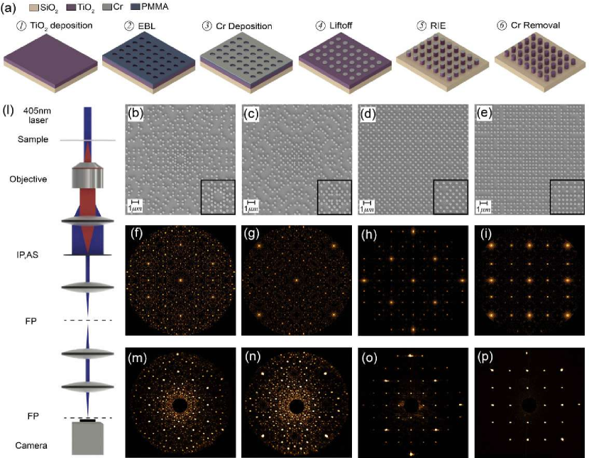
Figure 1: Experimental realization of sub-wavelength prime arrays and their diffractive properties. (a) Process flow used to fabricate the TiO₂ nanocylinders on a SiO₂ substrate. (b-e) SEM images of fabricated samples: panel (b-e) refer to Eisenstein, Gaussian, Hurwitz, and Lifschitz prime configurations, respectively. Insets: enlarged view of the central features for each pattern type. Nanocylinders have a 210 nm mean diameter, 250 nm height, and average inter-particle separation of 450 nm (see also Fig. S2). (l) Optical setup for measuring far-field diffraction patterns of laser illuminated sample. IP=Image Plane, AS=Aperture Stop, FP=Fourier Plane. Calculated (f-i) and measured (m-p) k-space intensity profiles corresponding to the prime arrays reported in panels (b-e), respectively.

When laser light illuminates the arrays at normal incidence, sub-wavelength pillars behave as dipolar scattering elements and the resulting far-field diffraction pattern is proportional to the structure factor defined by:

$$S(\bm{k})=\frac{1}{N}\Biggl{|}\sum_{j=1}^{N}e^{-i\bm{k}\cdot\bm{r}_{j}}\Biggr{|}^{2}$$ (1)

where $\bm{k}$ is the in-plane component of the wavevector and $\bm{r}_{j}$ are the vector positions of the $N$ nanoparticles in the array. This is demonstrated in Fig. 1 where we compare the calculated structure factors, shown in panels (f-i), with the measured diffraction patterns, shown in panels (m-p). The optical setup used to measure the diffraction is schematically illustrated in Fig. 1 (l) and further discussed in the Methods section. The experimental diffraction patterns match very well with the calculated ones and display sharp diffraction peaks embedded in a weaker diffuse background, particularly noticeable in the case of Gaussian and Eisenstein primes. The coexistence of sharp diffraction peaks with a continuous background is characteristic of singular continuous spectra described by singular functions that oscillate at every length scale Wang et al. (2018a); Baake and Grimm (2013). Systems with singular continuous spectra do not occur in nature and are generally associated to multifractal structures. See also Fig. S3 and the related discussion. The strength of the continuous spectral component weakens progressively from Eisenstein and Gaussian primes to Hurwitz and Lifschitz structures, which display a more regular geometry.

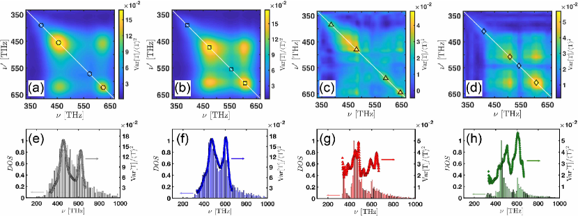
Figure 2: Frequency-frequency correlation analysis. (a-d) Frequency-frequency correlation matrix $C(\nu,\nu^{\prime})$ of Eisenstein, Gaussian, Hurwitz, and Lifschitz arrays, respectively. The different markers identify the frequency location of representative scattering resonances reported in Fig. 3. (e-f) Normalized variance as compared to the normalized density of states.

Multifractality is demonstrated by analyzing the local scale-invariance of the measured scattering resonances over a large range of scales. In contrast to traditional random media, where MF is achieved only close to the Anderson transition Richardella et al. (2010); Evers and Mirlin (2008); Faez et al. (2009), in complex prime arrays MF manifests over a much broader spectral range Wang et al. (2018a). To establish this fact experimentally, we collected multispectral images of the scattering resonances across the visible spectrum and analyzed their statistical correlations using the frequency-frequency correlation matrix Riboli et al. (2017):

$$C(\nu,\nu^{\prime})=\frac{\langle\delta I(\bm{r},\nu)\delta I(\bm{r},\nu^{\prime})\rangle}{\langle I(\bm{r},\nu)\rangle\langle I(\bm{r},\nu^{\prime})\rangle}$$ (2)

where $\bm{r}=(x,y)$ indicates the in-plane coordinates and $\delta I(\bm{r},\nu)=I(\bm{r},\nu)-\langle I(\bm{r},\nu)\rangle$ describes the fluctuations of the intensity with respect to the average value (see Supplementary Information). The degree of spatial similarity between different scattering resonances is directly quantified by the off-diagonal elements of matrix (2).

The results of the correlation analysis separate the set of collected scattering resonances into two spectral classes. The first class includes the Eisenstein and Gaussian arrays and is characterized by large fluctuations in the correlation matrix concentrated around two distinct spectral regions, as shown in Fig. 2 (a-b). In the second class, which includes the Hurwitz and Liftschitz arrays, the $C(\nu,\nu^{\prime})$ matrices are more structured and exhibit multi-scale fluctuations spreading over the entire frequency spectrum, as shown in Fig. 2 (c-d). This characteristic behavior indicates that the spatial intensity distributions of the measured scattered radiation rapidly fluctuate with frequency due to the excitation of scattering resonances in the systems (see Fig. S4). This is confirmed by comparing the behavior of the frequency-frequency correlation with the spectral behavior of the computed optical density of states (DOS) of the systems, which we obtained using the Green’s matrix spectral method (see Fig. S5 and detailed derivation in the Supplementary Information). Fig. 2 (e-h) presents the comparison between the DOS and the normalized variance $C(\nu,\nu)$ (see Methods). The Eisenstein and Gaussian prime arrays feature a DOS with two main peaks demonstrating that their scattering resonances are indeed located within the two spectral regions identified using the correlation analysis. On the other hand, the behavior of $C(\nu,\nu)$ and of the DOS for the Hurwitz and Lifschitz configurations features multiple spectral regions of strong intensity fluctuations.

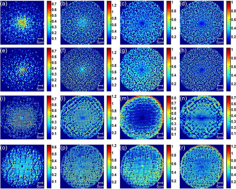
Figure 3: Direct observation of the scattering resonances of prime arrays. Representative multispectral dark-field images of the scattering resonances of Eisenstein, (a-d), Gaussian (e-h), Hurwitz (i-n), and Lifschitz (o-r) prime arrays. These quasi-modes are the scattering resonances that interact mostly with the structures and correspond to the spectral positions identified by the markers in Fig. 4 (a-d). These scattering resonances are normalized with respect to the transmission signal of a reference Ag-mirror.

We now investigate the spatial distributions of the measured scattering resonances within the two identified spectral classes. Fig. 3 shows representative dark-field images of the scattering resonances of Eisenstein (a-d), Gaussian (e-h), Hurwitz (i-n), and Lifschitz (o-r) arrays. Their spectral locations are labelled by the symbols in Fig. 2 (a-d) where different markers capture the main features identified using the correlation analysis. Specifically, the scattering resonances of the Eisenstein and Gaussian prime arrays, which belong to the first spectral class discussed above, display a clear transition from localization in the center of the arrays to a more extended nature in the plane of the arrays (see also Fig. S6). This scenario is far richer for the Hurwitz and Lifschitz configurations. In particular, the spatial distributions of their scattering resonances were found to be: (i) weakly localized around the central region of the arrays, (ii) localized at the edges of the arrays, and (iii) spatially extended over the whole arrays (more details provided in Figs. S6 and S7). The complex spatial distributions of the scattering resonances shown in Fig. 3 exhibit oscillations at multiple length scales, which are characteristic of critical modes in aperiodic systems with fractal and multifractal energy spectra. However, in order to quantitatively describe this behavior, we have analyzed the local scaling of the measured spatial intensity distributions using rigorous multifractal analysis Chhabra and Jensen (1989). In particular, we employ the box-counting method to characterize the size-scaling of the moments of the light intensity distribution. This is achieved by dividing the system into small boxes of varying size $l$. We then determine the minimum number of boxes $N(l)$ needed to cover the system for each size $l$ and evaluate the fractal dimension $D_{f}$ using the power-law scaling $N(l)\sim l^{-D_{f}}$. Traditional (homogeneous) fractal structures are characterized by a global scale-invariance symmetry described by a single fractal dimension $D_{f}$. On the other hand, heterogeneous fractals or multifractals are characterized by a continuous distribution $f(\alpha)$ of local scaling exponents such that $N(l)\sim l^{-f(\alpha)}$ Chhabra and Jensen (1989). The so-called singularity spectrum $f(\alpha)$ generalizes the fractal description of complex systems in terms of intertwined sets of traditional fractal objects. Different approaches are used to extract $f(\alpha)$ from the local scaling analysis. We have obtained the multifractal spectra directly from the dark-field measurements by employing the method introduced in ref. Chhabra and Jensen (1989). Details on the implementation are discussed in the Supplementary Information and in Fig. S7-S11.

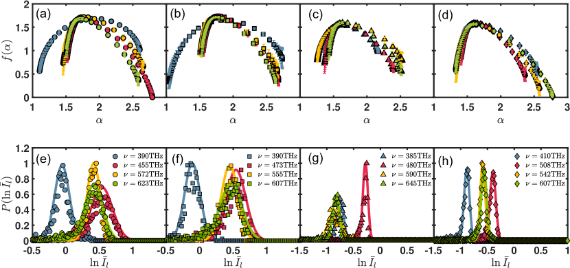
Figure 4: Multifractal nature of scattering resonances of prime arrays. Multifractal singularity spectra (a-d) and probability density functions of the box-integrated intensity $P(\ln I_{l})$ (e-h) of representative scattering resonances of Eisenstein (a,e), Gaussian (b,f), Hurwitz (c,g), and Lifschitz (d,h) prime arrays, respectively. Their resonance spectral positions are identified by the different markers of Fig. 2 (a-d). The continuous lines in panels (e-h) show the best fits obtained using log-normal function model.

Fig. 4 (a-d) demonstrate the multifractal nature of the measured scattering resonances of the prime arrays. All the singularity spectra $f(\alpha)$ exhibit a downward concavity with a large width $\Delta\alpha$, which is the hallmark of multifractality Chhabra and Jensen (1989). The behavior of the width $\Delta\alpha$ as a function of frequency reflects the previously identified classification in terms of the correlation matrix (see Fig. S9). In particular, the arrays with more significant intensity fluctuations, i.e. Eisenstein and Gaussian arrays, also display the broadest singularity spectra. Our findings establish a direct connection between the multifractal properties of the geometrical supports of the arrays (discussed in the Supplementary Information), the MF of the corresponding scattering resonances, and the singular continuous nature of diffraction patterns. To further characterize the MF of the scattering resonances we also computed, based on the experimental data, the mass exponent $\tau(q)$ and the generalized dimension $D(q)$, which provide alternative descriptions of multifractals. Multifractals are unambiguously characterized by a nonlinear $\tau(q)$ function and a smooth $D(q)$ function Stanley and Meakin (1988). This is reported in Fig. S8 and discussed in the Supplementary Information.

A direct consequence of multifractality is the non-Gaussian nature of the probability density function (PDF) of the light intensity distribution near, or at criticality Richardella et al. (2010); Faez et al. (2009). We have evaluated the PDF of the scattered radiation from the histogram of the logarithm of the box-integrated intensities, i.e. $P(\log[I_{l_{i}}])$. We show in Fig. 4 (i-l) the histograms produced by a box size of approximately $0.8\times\lambda$ where $\lambda$ is the wavelength in each case. We note that, although the intensity distributions of the scattering resonances in Fig. 3 show different degrees of spatial variations, all the PDFs are very-well reproduced considering log-normal distributions (continuous lines in Fig. 4 (e-h)). Moreover, we have verified that these findings do not depend on the box-counting size $l$, as shown in Fig. S10. Furthermore, the multifractal spectrum $f(\alpha)$ can be rigorously obtained from the PDF of the intensity within the parabolic approximation:

$$f(\alpha)=D_{f}-(\alpha-\alpha_{0})^{2}/4(\alpha_{0}-d)$$ (3)

where $D_{f}=f(\alpha_{0})$ is the fractal dimension of the geometrical support Faez et al. (2009). Equation (24) characterizes $f(\alpha)$ by the single parameter $\alpha_{0}$ associated to the mean $\mu$ and variance $\sigma$ of the PDF via the formula $\alpha_{0}=2\mu d/(2\mu+\sigma^{2})$. Deviations from the parabolic spectrum are associated to the strong MF of the scattering resonances of prime arrays across a broad range of frequencies (see Supplementary Information). The observed strong MF in the scattering resonances is uniquely associated to the multi-scale geometrical structure of prime arrays. In contrast, only weak MF was previously reported in uniform random scattering media at their metal-insulator Anderson transitions Richardella et al. (2010); Faez et al. (2009).

In conclusion, we have provided the first experimental observation of multifractality of classical waves in the optical regime by studying the resonances of photonic structures designed to reflect the intrinsic aperiodic order of complex primes and the irreducible elements of quaternion rings. Beyond its fundamental interest with respect to the discovery and characterization of multifractality in number theory Oliver and Soundararajan (2016); Wolf (1989), our findings establish a novel mechanism to transport and resonantly localize photons at multiple length scales and to enhance light-matter interactions with applications to active photonic devices and novel broadband nonlinear components. Moreover, the concepts developed in this work can be naturally transferred to quantum waves Bloch et al. (2012); Viebahn et al. (2019) and stimulate the development of novel quantum phases of matter and many-body phenomena that emerge from fundamental structures of algebraic number theory.

Methods

Sample fabrication

TiO₂ thin films were grown by reactive DC magnetron sputtering (MSP) on quartz (SiO₂) substrates with a Denton Discovery D8 Sputtering System. A 3 inch diameter Ti target (Kurt J. Lesker, 99.998$\%$) was used. The deposition was performed under a 200 Watt power at a 3.0 mTorr deposition pressure with a 1:3 Sccm flow rate ratio of O₂ to Ar gases. These growth conditions resulted in a deposition rate of about 1 nm/min. Chamber base pressure was kept below 5$\times$10${}^{-}7$ Torr, the target-substrate distance was fixed at 10cm, and substrates were rotated at a speed of 5 rpm. Substrates were solvent washed and plasma cleaned in O₂ prior to deposition.

The optical constants of the films were determined using a variable angle spectroscopic ellipsometer (V-Vase, J.A. Woollam) in the wavelength range of 300 nm to 2000 nm. The measured data were fitted in good agreement with the Cauchy model, an empirical relationship between refractive index and wavelength. The film thickness, verified with ellipsometry and scanning electron microscopy (SEM), was targeted at 250 nm.

Nanoparticle fabrication was performed with electron beam lithography. A PMMA resist layer of about 100 nm thickness was spun and baked before sputtering a thin conducting layer ($\sim$6 nm) of Au to compensate for the electrically insulating SiO₂ substrate. The resist was exposed at 30 keV by an SEM (Zeiss Supra 40) integrated with Nanometer Pattern Generation System direct write software. The sample was then developed in IPA:MIBK (3:1) solution for 70sec followed by a rinsing with IPA for 20sec. Next, a 20 nm thick layer of Cr was deposited on top of the developed resist with electron beam evaporation (CHA Industries Solution System). After this deposition, unwanted Cr was removed with a three minutes lift-off in acetone, and the nanoparticle patterns were transferred from the Cr mask to the TiO₂ thin film by reactive ion etching (RIE, Plasma-Therm, model 790) using Ar and SF₆ gases. Finally, the Cr mask was removed by wet etching in Transene 1020 Zheng et al. (2014).

Optical characterization

We measure the far-field diffraction pattern of laser light passing through the sample using the setup depicted in Fig. 2 (l). A 405 nm laser is focused onto the patterned area to overfill the pattern and to ensure uniformity in intensity across it. The forward scattered light is collected by a high numerical aperture objective (NA=0.9 Olympus MPlanFL N) which collects light scattered up to $64^{\circ}$ from the normal direction. A 4-F optical system, immediately behind the objective, creates an intermediate image plane and intermediate Fourier plane. An iris located at the intermediate image plane was used to restrict the light collection area only to the patterned region. A second 4-F optical system then re-images the intermediate Fourier plane onto the CCD (MediaCybernetics) with the appropriate magnification. Finally, digital filtering was employed to remove the strong D.C. component of the diffraction spectra to produce clear images. In order to measure the spatial distribution of the scattering resonances of prime arrays, we used a line-scan hyperspectral imaging system (XploRA Plus by Horiba Scientific). The field of view is illuminated by light from a lamp through the microscope objective. A line-like region of the field of view is projected into the spectrograph entrance slit. The slit image is then spectrally dispersed by means of a grating onto the camera image sensor. This allows the collection of all the spectra corresponding to a single line in the field of view. Scanning the sample with a stage then produces the hyperspectral image of the entire field of view. In our system, scanning 696 lines results in square-size hyperspectral image. The resolution of the CCD (Cooke/PCO Pixelfly PCI Camera) was set to be 430$\times$470, where 430 and 470 corresponds to a spatial and spectral resolution of 30 nm and 0.25 THz, respectively. The exposure time was set to be 1000 ms with a time interval of 1 min between different scanning lines. Finally, the dark-field data were normalized with respect to a reference signal of a Ag-mirror.

Correlation analysis

Each element $C(\nu_{i},\nu_{j})$ of the frequency-frequency correlation matrices of Fig. 4 (a-d) is the result of an average over $9\times 10^{4}$ correlated values. The normalization of the covariance $\langle\delta I(\bm{r},\nu)\delta I(\bm{r},\nu^{\prime})\rangle$ with respect to the product of the average values $\langle I(\bm{r},\nu)I(\bm{r},\nu^{\prime})\rangle$ minimizes the intrinsic spectral effects related to the illumination source of the experimental apparatus (see equation (2)). Each element of $C(\nu,\nu^{\prime})$ is a combination of spatial intrinsic fluctuations of the system’s parameters and extrinsic effects related to the illumination-collection efficiency and to the point spread function of the experimental apparatus. The spectral dependence of the extrinsic effects can be mitigated by the proper normalization of the correlations matrix Riboli et al. (2017). The white diagonal elements of Fig. 2 (a-d) as well as the continuous lines in Fig. 2 (e-h) are the normalized variance of the scattering resonances of prime arrays and are calculated by the equation:

$$C(\nu,\nu)=\frac{\langle\delta I(\bm{r},\nu)^{2}\rangle}{\langle I(\bm{r},\nu)\rangle^{2}}=\frac{\sigma^{2}(\nu)}{\mu^{2}(\nu)}$$ (4)

where $\mu(\nu)$ is the average value and $\sigma(\nu)$ is the standard deviation.

Multifractal analysis

The multifractal analysis of both structural and dynamical properties was performed from the corresponding 600 dpi bitmap image using the direct Chhabra-Jensen algorithm Chhabra and Jensen (1989) implemented in the routine FracLac (ver. September 2015) developed for the NIH distributed Image-J software package Schneider et al. (2012). This method is a useful tool to determine the scaling properties of a certain image, but has to be handled with care. First of all, the size of the boxes must satisfy some requirements. In the FracLac routine, the largest box should be larger than 50% but not exceed the entire image, while the smallest box is chosen to be the point at which the slope starts to deviate from the linear regime in the $\log(N)$ versus $\log(1/r)$ plot Schneider et al. (2012). Furthermore, the scattering resonance maps are not binary. Therefore, it is necessary to specify the threshold value above which the pixels are part of the object under analysis. Different calculations were performed for several threshold percentages (between 55% and 75%) of the maximum intensity of each scattering resonance of Fig. 3. Another source of error could be the scaling method used during the analysis. For each dark-field image we employed a linear, a rational, and a power scaled series of box sizes Schneider et al. (2012). All these aspects do not affect the main results of our paper, as shown by the error bars of Fig. 4 (a-d).

I Acknowledgements

All the authors would like to acknowledgment Dr. R.Wang for his contribution during the first stage of this work. All the authors would like to acknowledgment Dr. A. Ambrosio and Dr. M. Tamaglione for their help during the multispectral dark-field measurements performed at the Center for Nanoscale Systems at Harvard University (Cambridge, MA 02138 USA). F.S acknowledges Dr. F. Scazza for fruitful discussion on the applications of aperiodic lattices on ultracold quantum physics. L.D.N. acknowledges partial support from the Army Research Laboratory under Cooperative Agreement Number W911NF-12-2-0023 for the development of theoretical modeling.

Author contributions statement

F.S. performed numerical calculations, data analysis, organized the results, and contributed to the experimental measurements. S.G. performed Fourier spectra experiments, dark field measurements and contributed in numerical simulations. W.A.B. and R. Z. fabricated the samples. F.R. performed the correlation analysis. L.D.N. conceived, lead and supervised the research activities. L.D.N organized the results. L.D.N. and F.S. wrote the manuscript with critical feedback from all the authors. All authors contributed to discussions and manuscript revision.

II Supplementary Information

Multifractal analysis of prime arrays

The spatial distributions of the prime arrays considered in the paper are shown in Fig. 5 (a-d). The Eisenstein and Gaussian prime arrays, generated from the prime elements in the integer rings of complex quadratic fields, are characterized by a 12-fold and an 8-fold rotational symmetry, respectively. These features are evident from Fig. 5 (e-f) where we report their vector two-point correlation function $g_{2}(r,\theta)$, defined by:

$$g_{2}(r,\theta)dA=\frac{N_{exp}}{\rho}$$ (5)

where $\rho$ is the averaged point density and $N_{exp}$ refers to the expected number of points contained in the infinitesimal area $dA$=$rdrd\theta$ at position $(r,\theta)$. On the other hand, the Hurtwitz and Lifschitz configurations, obtained from two-dimensional cross section of the irreducible elements of quaternions, can be interpreted as the integer and the half-integer lattice points on a sphere of radius $\sqrt{N(z)}$ in $\mathbb{R}^{4}$, respectively. These lattice structures are evident in their $g_{2}(r,\theta)$, as shown in Fig. 5 (g-h). We refer to refs.Wang et al. (2018a); Vardi (1998); Rudnick and Waxman (2019); Prasad (2014); Conway and Smith (2003) for more details about the mathematical backgrounds to generate these point pattern distributions and to get more information on their geometrical properties.

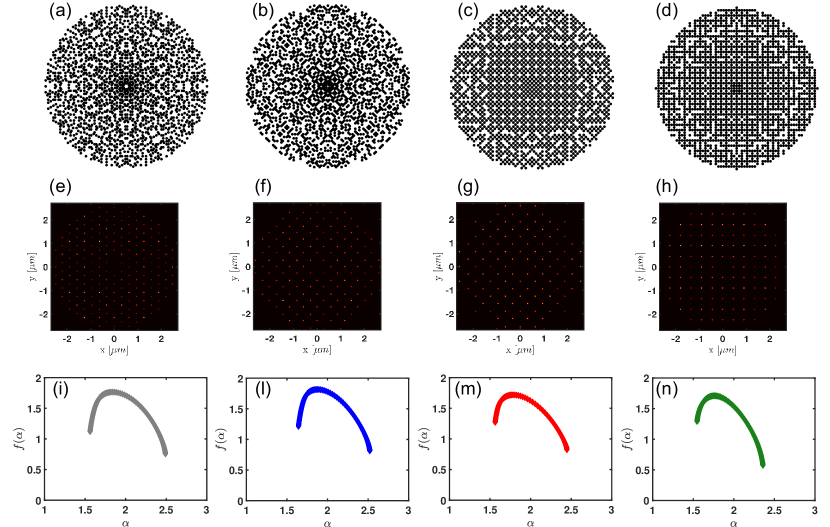
Figure 5: Geometrical properties of point patterns based on prime elements distributions. Prime point patterns generated by considering (a) N=2100 Eisenstein primes (EP), (b) N=2016 Gaussian primes (GP), (c) N=1957 Hurwitz primes (HP), and (d) N=2013 Lifschitz primes (LP).(e-h) Vector two-point correlation functions $g_{2}(r,\theta)$ of the prime arrays, and (i-n) singularity spectra $f(\alpha)$ corresponding to the respective array at the top of each column. The fractal dimensions $D_{f}$ are equal to 1.76, 1.82, 1.72, and 1.71 for the Eisenstin, Gaussian, Hurwitz, and Lifschitz geometry, respectively

To characterize the multifractal properties of prime elements in complex algebraic rings, we have applied the multifractal scaling analysis to the corresponding point patterns. As discussed in the manuscript, multifractal analysis is a statistical description that enables the study of long-term dynamical behavior of an arbitrary signal Chhabra and Jensen (1989); Hentschel and Procaccia (1983); Halsey et al. (1986); Meakin et al. (1985); Frisch and Parisi (1980); Hilborn et al. (2000); Nakayama and Yakubo (2013); Stanley and Meakin (1988); Mandelbrot (1983); Feder (2013). The idea of multifractality (MF), first introduced to analyze energy dissipation in turbulent fluids Frisch and Parisi (1980), widened our understanding of complex and intricate distributions observed in various fields of science Nakayama and Yakubo (2013). Specifically, multifractal analysis provided a number of significant insights into signal analysis Muzy et al. (1994), finance Mandelbrot et al. (1997); Schmitt et al. (2000); Schertzer et al. (1997), network traffic Riedi et al. (1999); Taqqu et al. (1997); Ribeiro et al. (2000), photonics Albuquerque and Cottam (2003); Trevino et al. (2012); Maciá (1999); Ryu et al. (1992); Sorensen (2001); Sroor et al. (2019); Desideri et al. (1989); Dal Negro and Boriskina (2012), and critical phenomena Richardella et al. (2010); Rodriguez et al. (2009); Zhao et al. (2019); Schreiber and Grussbach (1991); Evers and Mirlin (2008); Faez et al. (2009); Stanley and Meakin (1988); Mandelbrot (1983); Feder (2013); Stanley (1971), to cite a few.

Fig. 5 (i-n) report the results of this study. The geometrical supports of the prime arrays exhibit clear MF with singularity spectra $f(\alpha)$ of characteristic downward concavity which extends over a compact interval $[\alpha_{min},\alpha_{max}]$. Here, $\alpha_{min}$ (respectively $\alpha_{max}$) corresponds to the weakest (respectively the strongest) singularity. It is important to emphasize that if the geometrical support of an object is fractal (or multifractal), then also their dynamical properties (like their wavefunctions, energy spectra, and local density of states) exhibit fractality (multifractality) Nakayama and Yakubo (2013); Albuquerque and Cottam (2003); Trevino et al. (2012); Maciá (1999); Ryu et al. (1992); Kempkes et al. (2019). Interestingly, the opposite is not true. Indeed, electron wavefunctions and energy spectra at the frequency where the Anderson metal-insulator transition occurs have multifractal properties although electrons lie on an Euclidean (non-fractal) support Nakayama and Yakubo (2013); Schreiber and Grussbach (1991).

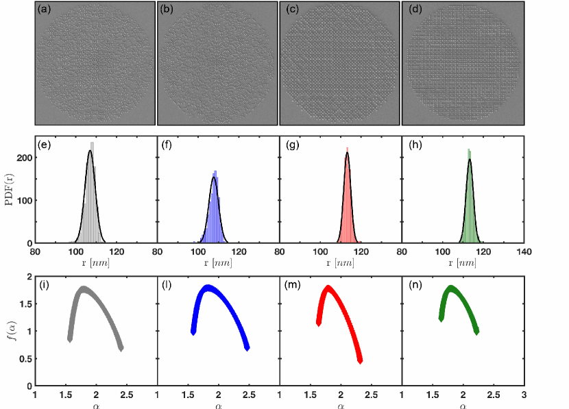
Figure 6: Geometrical properties of photonic prime arrays. Scanning Electron Microscope (SEM) of Eisenstein (a), Gaussian (b), Hurwitz (c), and Lifschitz configurations. (e-h) Nanocylinder size distributions of the corresponding prime arrays reported on top of each column evaluated from the SEM images by using the Image-J software package Schneider et al. (2012). (i-n) Singularity spectra $f(\alpha)$ of Eisenstin, Gaussian, Hurwitz, and Lifschitz geometry, respectively. The fractal dimensions $D_{f}$ are equal to 1.76, 1.79, 1.77, and 1.76, respectively.

In order to corroborate MF in the geometrical support of prime arrays, we have also applied multifractal scaling analysis to the SEM images of the fabricated TiO₂ nanoparticles deposited atop of a quartz substrate. Fig. 6 (a-d) show SEM images of the Eisenstein (a), Gaussian (b), Hurwitz (c), and Lifschitz (d) prime distributions. The fabricated nanocylinders have a 210 nm mean diameter, 250 nm height, and average inter-particle separation of 450 nm, as reported in Fig. 6 (e-d) that display histograms of the nanoparticle size distributions evaluated by using the ImageJ software package Schneider et al. (2012). These distributions show the traditional Gaussian profile (black-curves identify the Gaussian fits) associated to the random fluctuations of the electron beam and to the diffusion of the resist during the development. These results demonstrate the homogeneity of the size of the particles in the fabricated devices. Accordingly, the fabricated arrays display the same multifractal features of the point pattern distributions. The corresponding $f(\alpha)$ spectra are reported in Fig. 6 (i-n). Moreover, the Eisenstein and Gaussian prime arrays show a larger width $\Delta\alpha$, which describes the degree of inhomogeneity of the structures, compared to the Hurwitz and Lifschitz configurations. This is consistent with the more complex nature of their geometrical supports, as also reflected in the features of their $g_{2}(r,\theta)$.

As discussed in the main text, the MF of a geometrical object is also reflected in the singular continuous nature of its diffraction spectrum Baake and Grimm (2013, 2008). Although this cannot be rigorously proven, the singular continuous nature of the diffraction spectra can be shown by analyzing the cumulative integrated structure factor defined by the relation Wang et al. (2018a); Baake and Grimm (2013):

$$Z(k)=\int_{0}^{2\pi}\int_{0}^{k}S(q,\phi)qdqd\phi$$ (6)

The structure factor $S(\bm{k})$ of singular-continuous structures consist of bright peaks on a smooth and continuous background Wang et al. (2018a). Therefore, $Z(k)$, also named integrated intensity function, will exhibit sharp jumps connected by monotonically increasing intervals. Alternatively, its derivative $Z^{\prime}(k)$ consists of a non-zero baseline with intermittent spikes. All these features can indeed be observed for the all four prime arrays in Fig. 7 (a,b) when studying $Z(k)$ and $Z^{\prime}(k)$, respectively. An important aspect of this analysis is to make sure that the observed scaling curves are not dependent on the number of particles in the arrays. This is established in Fig. 7 where we report the scaling of $Z(k)$ and $Z^{\prime}(k)$ with respect to the size of the different prime arrays. Each curve in panels (a-b) is a superposition of four and nearly overlapping lines corresponding to different number of particles from 500 to 2000 elements (in intervals of 500). The small qualitative changes reported when varying the numbers of particles show that this analysis is very robust with respect to the size of the arrays and is indicative of their singular continuous nature.

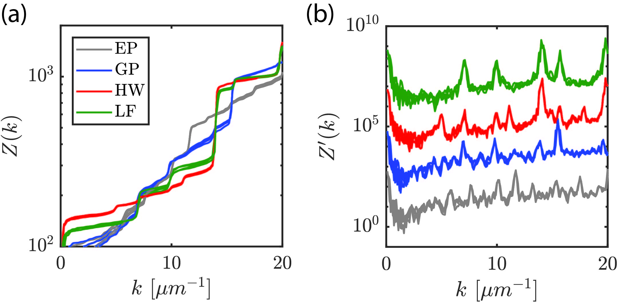
Figure 7: Integrated structure factor $Z(k)$ scaling analysis. (a) Z(k) and (b) $Z^{\prime}(k)$ for the four arrays. In (b) the GP, HW, and LF curves are vertically offest by factors of $10^{2}$, $10^{4}$, and $10^{6}$, respectively. The non-zero baseline of $Z^{\prime}(k)$ demonstrates the singular-continuous nature of the structures. In both plots there are four nearly-overlapping curves of each color, corresponding to different particle numbers in the array ranging from 500 to 2000 particles, showing that the result is insensitive to particle number.

Frequency-frequency correlation analysis.

Differently from the traditional random media where MF is achieved only close to the Anderson-transition Richardella et al. (2010); Evers and Mirlin (2008); Faez et al. (2009), in complex prime arrays MF is exhibited over a much broader spectral range Wang et al. (2018a). The frequency-frequency correlation matrices $C(\nu,\nu^{\prime})$, reported in Fig. 2 of the main manuscript, were used to establish a statistical and predictive relationship between the degree of similarity of all the measured dark-field scattering resonances. The degree of spatial similarity is measured by their off-diagonal elements Riboli et al. (2017). The main result of this analysis is the classification of prime arrays into two different classes, which reflects their mathematical structure. The first class comprises the Eisenstein and Gaussian (integers complex prime numbers) arrays, while the second one Hurtwitz and Lifschitz (generated from quaternions numbers) arrays. In the following we will discuss the relation between the $C(\nu,\nu^{\prime})$ results and the spatial features of the representative scattering resonances shown in Fig. 3 of the manuscript.

The first class is characterized by peak intensity fluctuations concentrated in two well-defined spectral regions located at $\nu\approx 460$THz and $\nu\approx 600$THz, respectively, with very similar absolute values close to $C(\nu,\nu)\approx 0.18$. Here, $C(\nu,\nu)$ indicates the normalized variance of the signal (see the main muascript for more details). In the present work, we didn’t evaluate the autocorrelation function due to the strong variations of the frequency dispersion of the scattering resonances of prime arrays Riboli et al. (2017). The off-diagonal peaks show that these large fluctuating resonances are correlated, indicating that their spatial distributions share common structural features. Moreover, a depletion of the intensity fluctuations is observed around $\nu\approx 550$THz in both Eisenstein and Gaussian arrays. All these features can be qualitatively observed also in the spatial distributions of the representative scattering resonances reported in Fig. 3 of the manuscript. Indeed, the Eisenstein and Gaussian configurations are characterized by a clear transition from modes localized in the center of the arrays to optical resonances more radially spreading in the plane of their geometrical supports. Specifically, Figs. 3 (a) and (c) do not share any common features: while the resonance (a) is more concentrated in the center of the arrays, resonance (c) is characterized by a minimum of the intensity in that region. On the other hand, the spatial distributions of panels (b) and (d) are correlated, as also shown by the off-diagonal peaks of the correlation matrix of Fig. 2 (a). The same conclusions are obtained in the Gaussian arrays: while the resonances (e) and (g) are not correlated, the spatial distributions (f) and (h) are similar.

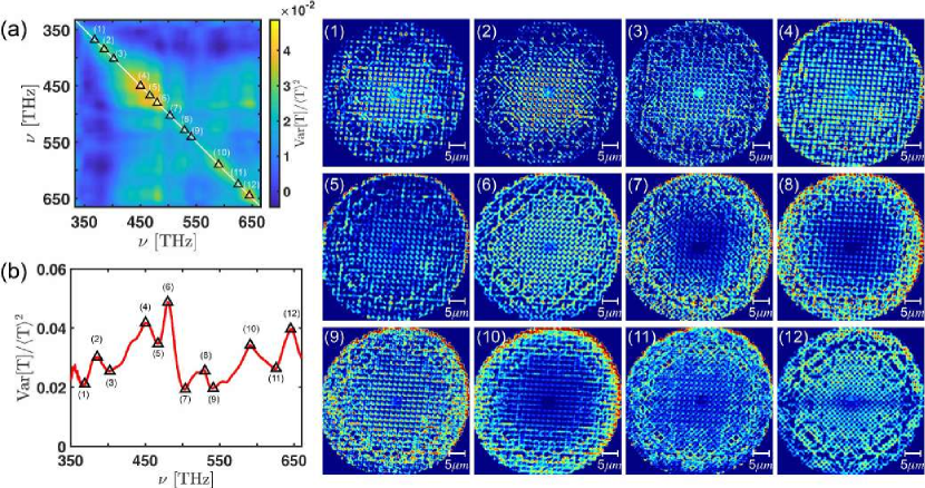
Figure 8: Frequency-frequency correlation of Hurwitz prime array. (a) Frequency-frequency correlation matrix $C(\nu,\nu^{\prime})$. (b) Normalized variance $C(\nu,\nu)$. The different numbers identify the spectral positions of 12 representative scattering resonances that are also reported in the figure.

The second class displays more variegated and richer correlation matrices. Specifically, their normalized variances are characterized by peaks and dips that spread over the entire measured frequency spectrum. This behavior indicates that their spatial distributions rapidly fluctuate with frequency. In the Hurwitz configuration, for example, some of these fast fluctuating resonances are correlated (or anti-correlated), as highlighted by the off-diagonal elements of the correlation matrix. Indeed, Fig. 8 shows that scattering resonances of the Hurwitz array can be classified in four different spectral regions: (i) [350,420] THZ (dark-field images 1-3), (ii) [430,480] THz (dark-field images 4-6), (iii) [480,600] THz (dark-field images 7-11), (iv) larger than 600 THz (dark-field image 12). Specifically, the region (i) is characterized by scattering resonances that are mostly concentered at the center of the array and that are anti-correlated with respect to the all the others, as shown in Fig. 8 (b). On the other hand, the spectral region (ii) is correlated with region (iv). The spectral region (iii), characterized by a minimum of the fluctuations of the scattered intensity, is populated by scattering resonances spatially localized at the edge of their geometrical support. Interestingly, these optical modes can be the analogues of the recently discovered topological edge states in aperiodic system Bandres et al. (2016); Wang et al. (2018b). The same considerations can be applied to the Lifschitz prime array. Though less noticeable, clear features of edge states can be recognized in Fig. 3 (q), which depicts a representative scattering resonance spectrally located in a minimum of its normalized variance. Furthermore, the scattering resonances (o) and (q) of Fig. 3 are not correlated in space, while (p) and (r) are correlated. This complex scenario is well-reproduced in our numerical simulations shown in Fig. 10 (see the next section for more details). Therefore, the quasi-modes of this second class display a more complex spatial structure as compared to Eisenstein and Gaussian arrays. In addition, the absolute value of their fluctuations ($C(\nu,\nu)\approx 0.05$) are smaller then the ones of the first class consistently with the more uniform nature of Hurwitz and Lifschitz arrays.

Electric and magnetic Green’s matrix method

In this section, we discuss an extension of the Green’s matrix spectral method Rusek et al. (2000), named electric and magnetic coupled dipole approximation (EMCDA) Dal Negro et al. (2019). This theoretical approach accounts for both the first-order Mie-Lorentz coefficients through the induced electric and magnetic polarizability Yurkin and Hoekstra (2007) and it provides valuable physical insights into the complex behavior on how light interacts with the aperiodic prime arrays. This approximation enables the simulation of the scattering response of large-scale photonic arrays with several thousand interacting particles, which are well beyond the reach of traditional numerical methods such as finite difference time domain (FDTD) or finite element method (FEM) techniques Dal Negro et al. (2019). The validity of this approximation depends on the scatterer material and the size parameter $kR$, where $k$ is the wavelength number and $R$ is the scatterer radius Dal Negro et al. (2019). In the following we briefly review some aspects of this formalism and we refer to Ref.Dal Negro et al. (2019) for a more detailed derivation and validation of this method.

The starting point to derive the EMCDA approximation is to evaluate the total electric and magnetic fields at the i-th particle location resulting from the electric and magnetic dipole moments of the j-th particle. These coupled equations can be written as:

$$\begin{bmatrix}\bm{E}_{i}\\ \bm{H}_{i}\end{bmatrix}=\begin{bmatrix}C_{ij}&-f_{ij}\\ f_{ij}&C_{ij}\\ \end{bmatrix}\begin{bmatrix}\tilde{\alpha}_{E}&0\\ 0&\tilde{\alpha}_{H}\\ \end{bmatrix}\begin{bmatrix}\bm{E}_{j}\\ \bm{H}_{j}\end{bmatrix},$$ (7)

where $\tilde{\alpha}_{E}$ and $\tilde{\alpha}_{H}$ are 3$\times$3 diagonal matrices containing the electric and magnetic polarizability $\alpha_{E}$ and $\alpha_{H}$Yurkin and Hoekstra (2007); Doyle (1989). The matrices $C_{ij}$ and $f_{ij}$ are defined by the relations

$$C_{ij}=\begin{bmatrix}a_{ij}+b_{ij}(n_{ij}^{x})^{2}&b_{ij}n_{ij}^{x}n_{ij}^{y}&b_{ij}n_{ij}^{x}n_{ij}^{z}\\ b_{ij}n_{ij}^{y}n_{ij}^{x}&a_{ij}+b_{ij}(n_{ij}^{y})^{2}&b_{ij}n_{ij}^{y}n_{ij}^{z}\\ b_{ij}n_{ij}^{z}n_{ij}^{x}&b_{ij}n_{ij}^{z}n_{ij}^{y}&a_{ij}+b_{ij}(n_{ij}^{z})^{2}\end{bmatrix}$$ (8)

$$f_{ij}=\begin{bmatrix}0&-d_{ij}n_{ij}^{z}&d_{ij}n_{ij}^{y}\\ d_{ij}n_{ij}^{z}&0&-d_{ij}n_{ij}^{x}\\ -d_{ij}n_{ij}^{y}&d_{ij}n_{ij}^{x}&0\end{bmatrix}$$ (9)

where $n_{ij}^{\beta}=\beta_{i}-\beta_{j}$ ($\beta=x,y,$ and $z$) are the components of the normal vector from the $jth$ to the $ith$ particle, while the coefficients $a_{ij}$, $b_{ij}$, and $c_{ij}$ are discussed in Refs.Dal Negro et al. (2019); Mulholland et al. (1994). These matrices define the electric and magnetic dyadic Green’s matrix $\overleftrightarrow{G}_{ij}$ that connects the electromagnetic field of the $i$-th-particle with the electromagnetic field of the $j$-th-particle:

$$\overleftrightarrow{G}_{ij}=\begin{bmatrix}C_{ij}&-f_{ij}\\ f_{ij}&C_{ij}\\ \end{bmatrix}=\begin{bmatrix}\overleftrightarrow{G}^{ee}_{ij}&\overleftrightarrow{G}^{eh}_{ij}\\ \overleftrightarrow{G}^{he}_{ij}&\overleftrightarrow{G}^{hh}_{ij}\\ \end{bmatrix}.$$ (10)

The dyadic symbol $\overleftrightarrow{\{\cdots\}}$ is used because we are taking into account all the field components. $\overleftrightarrow{G}_{ij}$ is a $6\times 6$ matrix. This formalism allows one to calculate the scattering, extinction, and absorption properties of an arbitrary geometry after applying a Foldy-Lax procedure Dal Negro et al. (2019) as discussed in the section “Scattering properties of prime arrays”.

The EMCDA method provides fundamental physical information about the light transport properties of open scattering media that cannot be easily accessed via FEM or FDTD techniques. Indeed, in contrast to numerical mesh-based methods, the EMCDA extension not only allows one to obtain the frequency positions and lifetimes of all the scattering resonances, but also to fully characterize their spectral statistics and measurable scattering parameters, such as the density of optical states (DOS) Wang et al. (2018a); Skipetrov (2019) reported in the Fig. 2 of the manuscript. Specifically, to include the magnetic dipole contribution inside the Green’s matrix spectral method, we have to isolate the traditional electric Green’s matrix $G_{ij}$, defined by the relation

$$G_{ij} =\frac{3}{2}\left(1-\delta_{ij}\right)\frac{e^{ik_{0}r_{ij}}}{ik_{0}r_{ij}}\Biggl{\{}\Bigl{[}\bm{U}-\hat{\bm{r}}_{ij}\hat{\bm{r}}_{ij}\Bigr{]}-$$

$$\Bigl{(}\bm{U}-3\hat{\bm{r}}_{ij}\hat{\bm{r}}_{ij}\Bigr{)}\left[\frac{1}{(k_{0}r_{ij})^{2}}+\frac{1}{ik_{0}r_{ij}}\right]\Biggr{\}}$$

Rusek et al. (1996); Lagendijk and Van Tiggelen (1996); Skipetrov and Sokolov (2014); Sgrignuoli et al. (2019a, b), by rewriting the matrix (8) in the compact form

$$C_{ij}=a_{ij}U+b_{ij}\hat{r}_{ij}\hat{r}_{ij}$$ (12)

where the term $\hat{r}_{ij}\hat{r}_{ij}$ has the explicit expression

$$\begin{bmatrix}(x_{i}-x_{j})^{2}&(x_{i}-x_{j})(y_{i}-y_{j})&(x_{i}-x_{j})(z_{i}-z_{j})\\ (x_{i}-x_{j})(y_{i}-y_{j})&(y_{i}-y_{j})^{2}&(y_{i}-y_{j})(z_{i}-z_{j})\\ (x_{i}-x_{j})(z_{i}-z_{j})&(y_{i}-y_{j})(z_{i}-z_{j})&(z_{i}-z_{j})^{2}\end{bmatrix}$$

divided by the factor $1/r^{2}_{ij}$. Equation (12) is then equivalent to

$$\begin{aligned} C_{ij}&=(1-\delta_{ij})\frac{e^{ik_{0}r_{ij}}}{r_{ij}}k_{0}^{2}\\ &\left[(U-\hat{r}_{ij}\hat{r}_{ij})-\left(\frac{1}{(k_{0}r_{ij})^{2}}+\frac{1}{ik_{0}r_{ij}}\right)(U-3\hat{r}_{ij}\hat{r}_{ij})\right]\\ &=\frac{2}{3}ik_{0}^{3}G_{ij}\end{aligned}$$

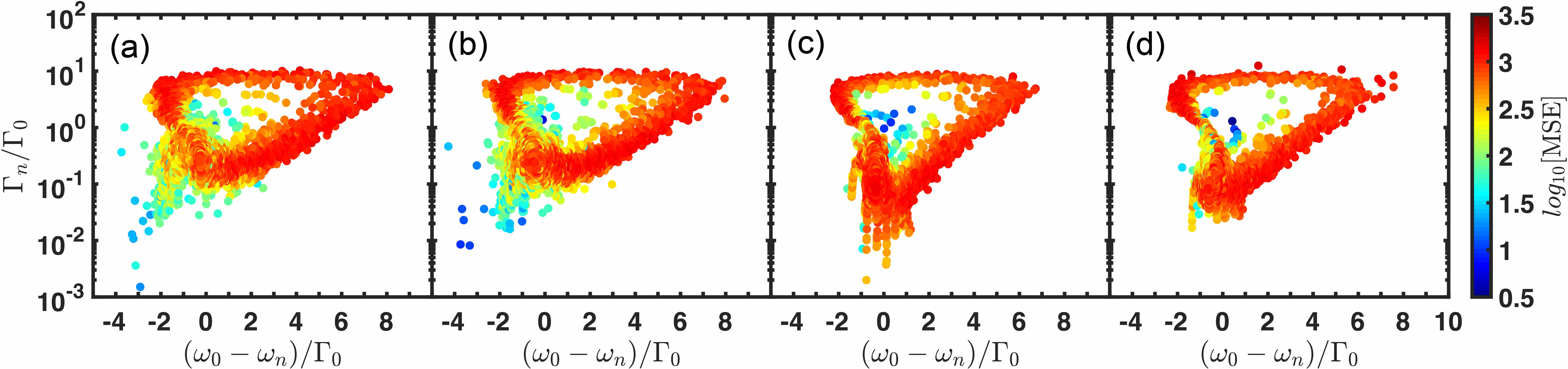
Figure 9: Spectral properties of the prime arrays. Eigenvalues of the electromagnetic Green’s matrix (15) are shown by point on the complex plane for almost 2000 electric and magnetic dipoles arranged in Eisenstein (a), Gaussian (b), Hurwitz (c), and Lifschitz (d) prime geometries. All these distributions are evaluated by fixing the optical density $\rho\lambda^{2}$ equal to 5. This value matches with the experimental conditions discussed in the main manuscript.

In the same way, matrix (9) can be rewritten in the compact form

$$f_{ij}=\frac{e^{ik_{0}r_{ij}}}{r_{ij}}k_{0}^{2}\left(1-\frac{1}{ik_{0}r_{ij}}\right)\hat{R}_{ij}$$ (13)

where

$$\hat{R}_{ij}=\begin{bmatrix}0&-\hat{r}^{z}_{ij}&\hat{r}^{y}_{ij}\\ \hat{r}^{z}_{ij}&0&-\hat{r}^{x}_{ij}\\ -\hat{r}^{y}_{ij}&\hat{r}^{x}_{ij}&0\end{bmatrix}$$

denotes the cartesian components of the unit directional vector $\hat{r}_{ij}=r_{ij}/|r_{ij}|$. Summarizing, the $6\times 6$ sub-blocks of the full Green’s matrix defined by equation (10) assumes the explicit form:

$$\begin{aligned} \overleftrightarrow{G_{ij}}&=\begin{bmatrix}\overleftrightarrow{G}^{ee}_{ij}&\overleftrightarrow{G}^{eh}_{ij}\\ \overleftrightarrow{G}^{he}_{ij}&\overleftrightarrow{G}^{hh}_{ij}\\ \end{bmatrix}=\\ &=\begin{bmatrix}\frac{2}{3}ik_{0}^{3}G_{ij}&-\Xi_{ij}\\ \Xi_{ij}&\frac{2}{3}ik_{0}^{3}G_{ij}\\ \end{bmatrix}\end{aligned}$$ (14)

where $\Xi_{ij}$ is equal to:

$$\frac{e^{ik_{0}r_{ij}}}{r_{ij}}k_{0}^{2}\left(1-\frac{1}{ik_{0}r_{ij}}\right)\hat{R}_{ij}$$

To be consistent with the notation of equation (Electric and magnetic Green’s matrix method), we have to multiply the matrix $\overleftrightarrow{G}_{ij}$ by the factor $3/2ik_{0}^{3}$ such that:

$$\frac{3}{2}\frac{1}{ik_{0}^{3}}\overleftrightarrow{G_{ij}}=\begin{bmatrix}G^{ee}_{ij}&G^{eh}_{ij}\\ G^{he}_{ij}&G^{hh}_{ij}\\ \end{bmatrix}$$ (15)

where $G^{ee}_{ij}=G^{hh}_{ij}=G_{ij}$ are defined by equation (Electric and magnetic Green’s matrix method), while the off-diagonal terms $G^{eh}_{ij}=-G^{he}_{ij}$ become

$$G^{he}_{ij}=\frac{3}{2}\frac{e^{ik_{0}r_{ij}}}{ik_{0}r_{ij}}\left(1-\frac{1}{ik_{0}r_{ij}}\right)\hat{R}_{ij}$$ (16)

The matrix (15) is a non-Hermitian matrix. As a consequence, it has complex eigenvalues $\Lambda_{n}$ with a physical interpretation related to the scattering frequency and decay time. Fig. 9 shows the eigenvalue distributions produced by numerically diagonalizing the matrix (15) made from more than 2000 electric and magnetic dipoles arranged in the Eisenstein (a), Gaussian(b), Hurwitz (c), and Lifschitz (d) geometries. These complex pole distributions are color coded according to the $\log_{10}$ values of the mode spatial extent (MSE). The MSE characterizes the spatial extent of a photonic mode Sgrignuoli et al. (2015). All these data are obtained by fixing the optical density $\rho\lambda^{2}$ equal to 5. Here $\rho$ is the number of particles per unit area while $\lambda$ in the optical wavelength. This value is compatible with our experimental conditions discussed in the main manuscript. Moreover, the distribution of level spacing calculated from the eigenvalues of the matrix (Electric and magnetic Green’s matrix method) is reproduced by the critical cumulative probability distribution at this optical regime Wang et al. (2018a). This feature is confirmed by the main result of our manuscript: MF characterizes the scattering resonances of prime arrays over a broad frequency range.

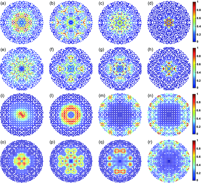
Figure 10: Calculated scattering resonances of the prime arrays. Representative spatial distributions of the electromagnetic Green’s matrix eigenvectors produced by approximately 2000 electric and magnetic point dipoles arranged in Eisenstein (a-d), Gaussian (e-h), Hurwitz (i-n), and Lifschitz (o-r) prime arrangement, respectively.

A peculiar feature is shown in Fig. 9: the existence of spectral gaps. This characteristic, which does not occur in traditional random arrays, reflects the role played by the structural correlations of prime arrays and becomes prominent in the DOS behavior. The DOS distributions are calculated from the histograms of the real part of the eigenvalue of the matrix (15). Within the Green’s formalism, the size and the refractive index of the particles can be taken into account after the diagonalization of the Green’s matrix by extracting the frequency $\omega_{0}$ and the decay rate $\Gamma_{0}$ from the central position and the lineshape of the scattering cross section of a single particle. In the present case, we have extracted these parameters from the scattering cross section of a single TiO₂ nanoparticle of 105 nm radius embedded in an effective refractive index medium ($n\sim 2.5$) to emulate the presence of the quartz substrate. Although the relation between the fluctuations of scattered intensity and the DOS is not trivial because it depends on many intrinsic and extrinsic factors Yasumoto (2005), the results of Fig. 2 show qualitative agreement confirming the analysis provided by the frequency-frequency correlation matrix $C(\nu,\nu^{\prime})$.

The spatial distribution of the scattering resonances can be evaluated by analyzing the eigenvectors of the matrix (15). Representative scattering resonances of prime arrays are reported in Fig. 10. These quasi-modes populate the region of the complex plane near the spectral gaps and are characterized by a low decay rates ($\Im[\Lambda_{n}]<1$) and a high value of the mode spatial extent ($\log_{10}$[MSE]$>1.5$). These eigenvectors are critical scattering resonances because they are long-lived and extended quasi-modes Wang et al. (2018a). Moreover, they show the same characteristic of the experimental dark-field images reported in the main manuscript. Specifically, the scattering resonances of Eisenstein (a-d) and Gaussian (e-h) configurations display a clear transition from quasi-modes localized at the center of the arrays to resonances more radially spread around the plane of their geometrical supports. Furthermore, band-edges scattering resonances are clearly visible in both the Hurtwitz and Lifschitz array.

Multifractal Analysis of the scattering resonances of the prime arrays

We have used the very well know FracLac routine, developed for the Image-J software package Schneider et al. (2012), to perform the multifractal analysis presented and discussed in the main manuscript. This routine is based on the method introduced in Ref.Chhabra and Jensen (1989). In the following, we will review how evaluate the singularity spectrum $f(\alpha)$, the generalized dimensions $D_{q}$, and the mass exponent $\tau(q)$ from the binary map of a representative scattering resonance reported in Fig. 11 (a-b). These parameters are calculated by using the box-counting method and are used to discriminate if a certain distribution is non fractal, fractal, or multifractal.

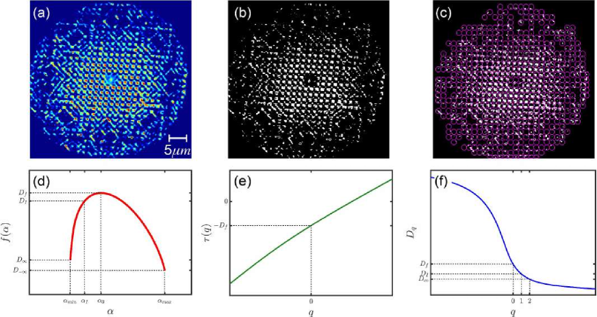
Figure 11: Multifractal analysis: method overview. (a) Selected scattering resonance produced by the Hurwitz prime array at the frequency $\nu=387$THz. (b) Corresponding 600dbi bitmap image. (c) Box counting discretization. Multifractal exponents are evaluated by using the direct Chhabra-Jensen algorithm Chhabra and Jensen (1989) implemented in the FracLac routine Schneider et al. (2012). Specifically, panel (d), (e), and (f) displays the multifractal singularity spectrum $f(\alpha)$, the mass exponent $\tau(q)$, and the generalized dimensions $D_{q}$, respectively.

As discussed in the main manuscript, the idea of the box-counting method is to divide the space embedding the object into a hyper-cubic grid of boxes of size $l$, as shown in Fig. 11 (c) for a representative Hurwitz scattering resonance. In inhomogeneous systems, the probability $P_{i}(l)$, calculated as the integral of the measure over the $i^{th}$ box, scales as $P_{i}(l)\sim l^{\alpha_{i}}$, where $\alpha_{i}$ are named Lipschitz-Holder exponents and quantify the strength of the singularity of a measure inside the $i^{th}$ box. Similar $\alpha_{i}$ values can be found at different positions within a distribution of boxes. The number of boxes $N(l)$, where $P_{i}$ has singularity strength $\alpha$ between $\alpha$ and $\alpha+d\alpha$, scales as $N(l)\sim l^{-f(\alpha)}$ Chhabra and Jensen (1989); Halsey et al. (1986); Schreiber and Grussbach (1991). The fact that the subset specified by $\alpha_{i}$ has its own fractal dimension $f(\alpha_{i})$ explains the etymology of the word multifractal.

Multifractal sets can also be described by a parameter called generalized dimensions $D_{q}$. This parameter was proposed for the first time as a different measure to describe the “strangeness” of some phase space of dissipative dynamical systems, called attractors, which exhibit chaotic behavior Grassberger and Procaccia (1983). There are three dimensions that characterize $D_{q}$: the capacity dimension $D_{0}$, the information dimension $D_{I}$, and the correlation dimension $D_{co}$ Mandelbrot (1977); Hentschel and Procaccia (1983). The capacity dimension is independent from $q$ and provides global information of a system, i.e. D₀ coincides with the box-counting dimension $D_{f}$ Hilborn et al. (2000); Voss (1988). On the other hand, $D_{I}$ is related to the information or Shannon entropy and quantifies the degree of disorder present in a distribution Mandelbrot (1977); Chhabra and Jensen (1989); Gouyet (1996). $D_{co}$, which is mathematically equivalent to the correlation integral Grassberger and Procaccia (1983), computes the correlation of measures contained in the intervals of size $l$. The relation between these three measures is $D_{co}\leq D_{I}\leq D_{0}$, where the three are equal only in the case of homogeneous fractals Korvin (1992). The generalized dimension is related to the scaling of the $q^{th}$ moments of a distribution and it is defined as:

$$D_{q}=\frac{1}{q-1}\lim_{l\rightarrow 0}\Biggl{[}\frac{\log\mu(q,l)}{\log l}\Biggr{]}$$ (17)

where $\mu(q,l)$ is equal to

$$\mu(q,l)=\sum_{i}P_{i}(l)^{q}\sim l^{-\tau(q)}$$ (18)

Equation (18) can be interpreted in the following way: if the $q^{th}$ moments of $P_{i}(l)$ are proportional to some power $\tau(q)$ of the box size $l$, then $\mu(q,l)$ distinguishes intertwined regions which scale in different ways according to the exponent $\tau(q)$, also named mass exponent Schreiber and Grussbach (1991). Specifically, $\tau(q)=(q-1)D_{q}$ shows how the moments of a given distributions scale with the box size $l$. If $\tau(q)$ is a nonlinear function of $q$, we call the distribution of measures multifractal Schreiber and Grussbach (1991); Nakayama and Yakubo (2013).

The two exponents $f(\alpha)$ and $\tau(q)$ are related to each other by means of a Legendre transformation Chhabra and Jensen (1989); Halsey et al. (1986); Schreiber and Grussbach (1991); Nakayama and Yakubo (2013):

$$\tau(q) =\alpha(q)q-f[\alpha(q)]\leavevmode\nobreak\ \leavevmode\nobreak\ \leavevmode\nobreak\ \leavevmode\nobreak\ \mbox{where}\leavevmode\nobreak\ \leavevmode\nobreak\ q=\frac{df(\alpha)}{d\alpha}$$ (19)

$$f(\alpha) =q(\alpha)-\tau[q(\alpha)]\leavevmode\nobreak\ \leavevmode\nobreak\ \leavevmode\nobreak\ \leavevmode\nobreak\ \leavevmode\nobreak\ \leavevmode\nobreak\ \mbox{where}\leavevmode\nobreak\ \leavevmode\nobreak\ \alpha=\frac{d\tau(q)}{dq}$$

This relationship reflects a deep connection with the thermodynamic formalism of statistical mechanics where $\tau(q)$ and $q$ are conjugate thermodynamic variables to $f(\alpha)$ and $\alpha$ Chhabra and Jensen (1989). In this context, the function $\mu(q,l)$ is formally analogous to the partition function $Z(\beta)$, while $\tau(q)$ can be interpreted as the free energy. Its Legendre transform $f(\alpha)$ is thus the analogue of the entropy, while $\alpha$ is the energy $E$. Notably, the characteristic shape of $f(\alpha)$ in the parabolic approximation (see following sections for more details) resembles the functional dependence of the entropy from $E$.

In order to evaluate these exponents, we can derive $\tau(q)$ from the log-log plot of $l$ versus $\mu(q,l)$ by using a least-fit square method. Then, $D_{q}$ and $f(\alpha)$ can be obtained from equations (17) and (19), respectively. However, the derivation of $f(\alpha)$ through the Legendre transformation suffers from numerical inaccuracies related to the differentiation to obtain the coefficients $\alpha$ Schreiber and Grussbach (1991); Nakayama and Yakubo (2013); Chhabra and Jensen (1989). In order to overcome these numerical errors, the Chhabra-Jensen method can be implemented. This method computes $f(\alpha)$ directly from the data Chhabra and Jensen (1989). By defining the one parameter family $\hat{\mu}_{i}(q,l)$ through the relation:

$$\hat{\mu}_{i}(q,l)=\frac{P_{i}(l)^{q}}{\sum_{j}P_{j}(l)^{q}}$$ (20)

the singularity strength $\alpha$ and the multifractal spectrum $f(\alpha)$ are given by:

$$\alpha=\lim_{l\rightarrow 0}\frac{\sum_{i}\hat{\mu}_{i}(q,l)\log[P_{i}(l)]}{\log l}$$ (21)

$$f[\alpha(q)]=\lim_{l\rightarrow 0}\frac{\sum_{i}\hat{\mu}_{i}(q,l)\log[\hat{\mu}_{i}(q,l)]}{\log l}$$ (22)

Specifically, the numerators of equations (21) and (22) are evaluated for each value of $q$ for decreasing box sizes. $f[\alpha(q)]$ and $\alpha(q)$ are then extrapolated from the slopes of the plots of $\sum_{i}\hat{\mu}_{i}(q,l)\log[\hat{\mu}_{i}(q,l)]$ and $\sum_{i}\hat{\mu}_{i}(q,l)\log[P_{i}(l)]$ versus $\log l$, respectively. Therefore, $\alpha$ and $f(\alpha)$ are calculated directly from the data by performing a box-counting procedure. More details on the explicit derivation of equations (21) and (22) can be found in Refs.Nakayama and Yakubo (2013); Chhabra and Jensen (1989); Schreiber and Grussbach (1991).

Fig. 11 (d) shows a representative multifractal spectrum evaluated by using the method explained above. Fig. 11 (d) displays a singularity spectrum which is multifractal, i.e. smooth downward concavities with a finite width $\Delta\alpha=\alpha_{max}-\alpha_{min}$. The mass exponent $\tau(q)$ can be also evaluated directly from Fig. 11 (c), as discussed above. Fig. 11 (e) displays the non-linear dependence of the mass exponent, demonstrating that the representative scattering resonance of panel (a) is characterized by intertwined fractal sets that scale in different ways. Notice that the moment $q=0$ corresponds to the maximum of the spectrum yielding $f(\alpha_{0})=D_{f}$. Finally, from the knowledge of $\tau(q)$, the generalized dimensions $D_{q}$ can be easily calculated by the relation $D_{q}=\tau(q)/(q-1)$, as reported in panel (f).

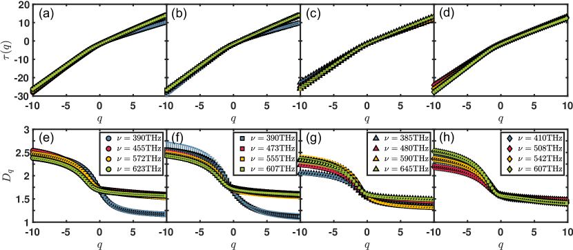
Figure 12: Alternative multifractal hallmarks. Mass exponent $\tau(q)$ (a-d) and generalized dimensions $D_{q}$ (e-h) of the representative scattering resonances of the prime arrays discussed in Fig. 3 of the main manuscript.

Mass exponent, generalized dimensions, $\Delta\alpha$, and PDF fit trends

Table 1: Generalized dimensions. Fractal ($D_{f}$), information ($D_{I}$), and correlation ($D_{co}$) dimensions of the representative scattering resonances discussed in the main manuscript.

	$D_{f}$	$D_{I}$	$D_{co}$
EP	(1.69,1.71,1.72,1.68)	(1.55,1.70,1.67,1.65)	(1.36,1.68,1.64,1.64)
GP	(1.65,1.74,1.69,1.72)	(1.54,1.71,1.66,1.68)	(1.39,1.69,1.64,1.67)
HP	(1.54,1.57,1.55,1.60)	(1.47,1.53,1.46,1.56)	(1.44,1.51,1.42,1.54)
LP	(1.57,1.59,1.58,1.57)	(1.53,1.56,1.54,1.54)	(1.51,1.54,1.52,1.53)

The exponent $\tau(q)$, as discussed in the previous section, describes the scaling of the partition function $\mu(q,l)$ with respect to box size $l$ and defines the generalized dimension through the relation $D(q)=\tau(q)/(q-1)$. Multifractals are unambiguously characterized by nonlinear $\tau(q)$ functions Stanley and Meakin (1988) and a smooth $D(q)$ function Hentschel and Procaccia (1983). This is reported in Fig. 12 (a-d) for $\tau(q)$ and (e-h) for $D(q)$, demonstrating the multifractal nature of dark-field images of Fig. 3 of the main manuscript. Moreover, Table 1 reports the capacity, the information, and the correlation dimensions for all the analyzed scattering resonances. These values are in agreement with the main results discussed in the manuscript. In particular, the information dimension is always larger for the Eisenstein and Gaussian arrays. This is consistent with the more inhomogeneous nature of these arrays with respect to the Hurwitz and Lifschitz arrays.

Also of interest are the $\Delta\alpha$ trends extrapolated from the multifractal spectra of Fig. 4 (a-d) and reported in Fig. 13. $\Delta\alpha$ is a parameter related to the inhomogeneity of a system Richardella et al. (2010) and it displays, as a function of the frequency, similar features in the Eisenstein and Gaussian configuration as well as in the Hurtwitz and Liftschitz arrays resembling the classification of the prime arrays in two different classes. Indeed, while a trend from large to small $\Delta\alpha$ values is observed in the Eisenstein and Gaussian configuration, the $\Delta\alpha$ of the scattering resonances of Hurtwitz and Liftschitz arrays shows the opposite behavior.

Finally, Fig. 14 plots the peak-position and the width of the histogram of the logarithm of the box-integrated intensity, normalized with respect to their averaged values, as a function of the box size $l=b\lambda$. These results demonstrate the stability of the non-Gaussian nature of the PDF reported in Fig. 4 (e-h). Moreover, the peaks of these PDFs are always shifted from their averaged intensity resembling the criticality near the Anderson transition of ultrasound waves Faez et al. (2009).

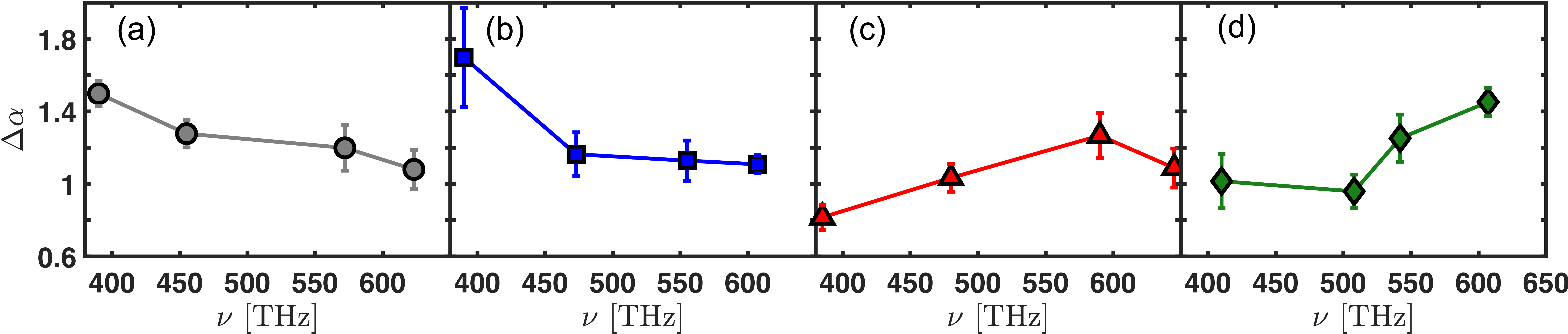
Figure 13: $\Delta\alpha$ characterization. The width $\Delta\alpha$=$\alpha_{max}-\alpha_{min}$ of the multifractal spectra of Eisenstein (a), Gaussian (b), Hurwitz (c), and Lifschitz (d) arrays are reported as a function of the frequency. Here $\alpha_{min}$ (respectively $\alpha_{max}$) corresponds to the weakest (respectively the strongest) singularity.

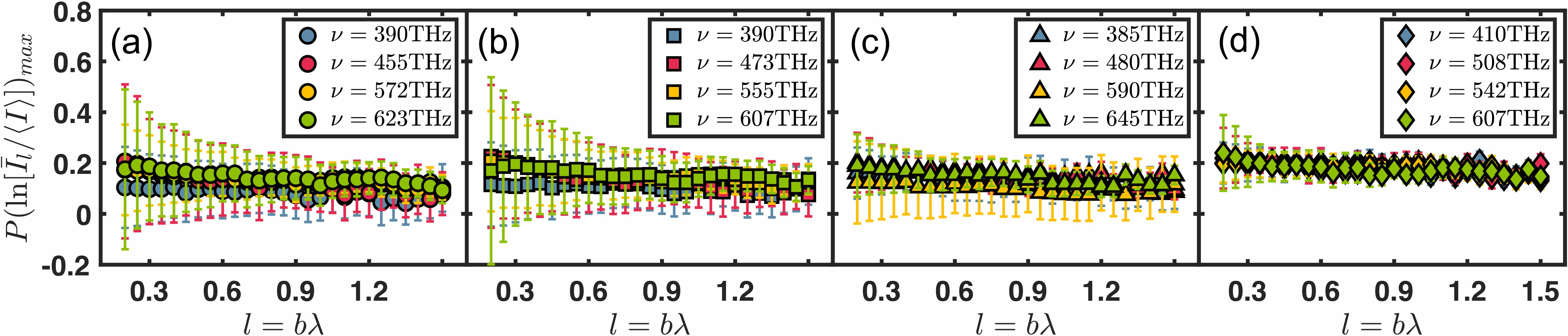
Figure 14: Results of intensity PDF fits. The peak position (symbols) and the full width half maximum (bars) of the intensity histograms, normalized with respect to their averaged values, with respect to their averaged values are plotted for Eisenstein (a), Gaussian (b), Hurwitz (c), and Lifschitz (d) arrays as a function of the box size $l$ for different frequencies corresponding to the main features of their correlation matrices $C(\nu,\nu^{\prime})$.

Parabolic approximation of $f(\alpha)$

Taking inspiration from the physics of the metal-insulator transition occurring in disordered electron systems Richardella et al. (2010); Schreiber and Grussbach (1991); Evers and Mirlin (2008) and from its elastic wave counterpart Faez et al. (2009), we discuss in this section the consequences of the parabolic approximation applied to the scattering resonances of the prime arrays. As discussed in the main manuscript, first order perturbation theory for an Anderson transition in $2+\epsilon$ dimensions Wegner (1980), produces the parabolic approximation to describe the multifractal nature of its wave functions Wegner (1980); Aoki (1983); Castellani and Peliti (1986). As a consequence, an infinite set of exponents, contrary to the usual situation occurring in standard critical phenomena where only two independent exponents are required Stanley (1971), have to be considered. Therefore, this critical transition is accompanied by a broadening of distributions of physical quantities governed, no longer by a unique length scale, but by a distribution of them Ioffe et al. (1985).

To understand this approximation is sufficient to remember that the multifractal analysis can be operationally implemented considering the power law behaviors of the q-th power of multiresolution structure quantities $S(q,a)\sim{a^{\zeta(q)}}$ that depend on $q$ as well as on the analysis scale $a$. The scaling exponent $\zeta(q)$ is ten expanded to a polynomial as:

$$\zeta(q)=c_{1}q+c_{2}q^{2}/2+c_{3}q^{3}/6+\cdots$$ (23)

The meaning of equation (23) is the following: (i) if $\zeta(q)$ is a linear function of $q$, then the distribution is fractal; (ii) if $\zeta(q)$ is a quadratic function of $q$ (i.e. parabolic function of $q$), then the distribution is called weak multifractal Faez et al. (2009); (iii) if $\zeta(q)$ is characterized by higher $q$ moments, then the distribution is multifractal in the strong sense.

In order to test the deviation of an arbitrary $f(\alpha)$ with respect to the parabolic approximation:

$$f(\alpha)=D_{f}-(\alpha-\alpha_{0})^{2}/4(\alpha_{0}-d)$$ (24)

we can derive a relation between the singularity spectrum and the probability distribution function of the corresponding measure Nakayama and Yakubo (2013). Denoting a distribution function of box measures $\mu_{b}$, grained by a box of size $l_{i}$, with $P(\mu_{b},\delta_{i})$ ($\delta_{i}=l_{i}/L$ where $L$ is the system size), $P(\mu_{b},\delta_{i})d\mu_{b}$ expresses the number of boxes that have $\mu_{b}$ lying in the interval $[\mu_{b},\mu_{b}+d\mu_{b}]$. By defining the exponents $\alpha_{i}=\log\mu_{b}/\log\delta_{i}$ and if $\delta_{i}$ are small, we can replace $P(\mu_{b},\delta_{i})$ with the distribution function $\bar{P}(\alpha_{i},\delta_{i})$ such to define the expression $K(\log\mu_{b},\delta_{i})$ through the relation:

$$K(\log\mu_{b},\delta_{i})=\frac{\bar{P}(\alpha_{i},\delta_{i})}{\log\delta_{i}}\approx e^{f(\alpha_{i})\log\delta_{i}}$$ (25)

where we have used $\bar{P}(\alpha_{i},\delta_{i})=\rho(\alpha_{i})\delta_{i}^{-f(\alpha_{i})}$ ($\rho(\alpha_{i})$ is the density of boxes with exponent $\alpha_{i}$) and the fact that both $\rho(\alpha_{i})$ and $1/\log\delta_{i}$ are weaker than $\delta_{i}^{f(\alpha_{i})}$ for small $\delta_{i}$ Nakayama and Yakubo (2013).

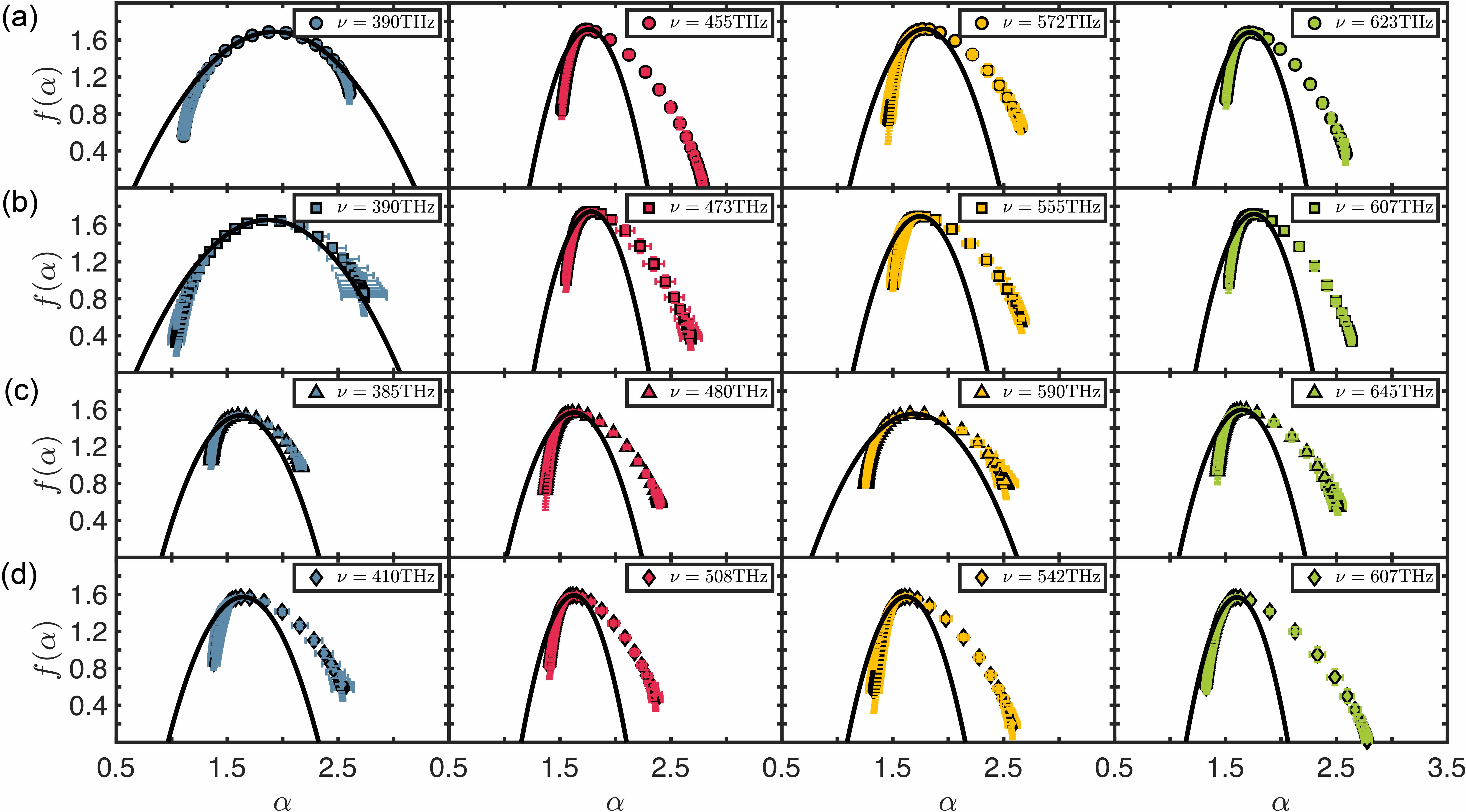
Figure 15: Parabolic approximation. The parabolic approximation (black lines) is compared with respect to the multifractal spectra (symbols) evaluated directly from the experimental dark-field images of Fig. 3 of the main paper.

Substituting equation (24) into equation (25) and introducing a normalization factor $N(\delta_{i})$, the distribution function $K(\log\mu_{b},\delta_{i})$ can be re-written as:

$$\begin{aligned} K(\log\mu_{b},\delta_{i})&=\frac{1}{N(\delta_{i})}\exp\{-f(\alpha_{i})\log\delta_{i}\}\\ &=\frac{1}{N(\delta_{i})}\exp\left\{\left[D_{f}\frac{(\alpha_{i}-\alpha_{0})^{2}}{4(\alpha_{0}-D_{f})}\right]\log\delta_{i}\right\}\\ \end{aligned}$$

$$\sim\exp\left\{\frac{(\log\mu_{b}-\alpha_{0}\log\delta_{i})^{2}}{4(\alpha_{0}-D_{f})\log\delta_{i}}\right\}$$ (26)

This is a log-normal distribution function. Indeed, considering that $\log\delta_{i}<0$ and defining $x=\mu_{b}$, $\bar{x}=-\alpha_{i}|\log\delta_{i}|$, and $\sigma=\sqrt{2(\alpha_{0}-D_{f})|\log\delta_{i}|}$, equation (Parabolic approximation of $f(\alpha)$) can be rewritten in the from

$$K(\log\mu_{b},\delta_{i})\sim\exp\left\{-\frac{(\log x-\bar{x})^{2}}{2\sigma^{2}}\right\}$$ (27)

Equation (27) allows to evaluate the parameter $\alpha_{0}$, that characterizes the parabolic approximation (24), through the log-normal fit of the probability density function associated to the box measure $\mu_{b}$.

Fig. 15 shows the deviation of the multifractal spectra $f(\alpha)$ of representative scattering resonances of prime arrays from their parabolic approximation. Here the box measures $\mu_{b}$ are the integrated intensities $I_{l_{i}}$. Notice that the black curves of Fig. 15 are not fits but are produced by evaluating equation (24) with the different single parameters $\alpha_{0}$ derived from the fit results reported in Fig. 4 (e-h). As clearly shown in Fig. 15, the parabolic approximation reproduces very well the “true” $f(\alpha)$ spectra quite well near $\alpha=\alpha_{0}$ but deviates significantly away from it. This implies that our data cannot be reproduced by taking into account only the quadratic term of the expansion (23). Therefore, our results demonstrate the strong multifractal character of the optical resonances of the prime arrays.

Scattering properties of prime arrays

In this section we report the analysis of the scattering spectra of prime arrays. Dark-field (DF) microscopy measurements were performed using the experimental setup sketched in Fig. 16 (a). A 75W Xenon lamp (Olympus U-LH75XEAPO) illuminates an Olympus Darkfield Condenser with numerical aperture (NA) of 0.8-0.92 (U-DC9) which is focused onto the arrays. The incident angle cone of illumination was approximatively of $15^{\circ}$ with respect to the normal of the array plane. The scattered light was collect with a 0.75 NA Objective (Olympus MPLA-N) then split by a 50/50 beam splitter. On one path, the light was focused onto a CCD array to produce the dark-field images reported in Fig. 16 (b-e). On the other path, an image was formed onto an iris to restrict the collected light to that of a single array, and then focused into an Ocean Optics (QE65000) fiber coupled spectrometer to generate the dark-field scattering spectra shown in Fig. 16 (f-i). All the scattering spectra were background corrected by subtraction of the scattering signal from an equal-size unpatterned area adjacent to each prime array. In order to couple light through the microscope objective with no sample in place, the DF objective was severely defocused. Moreover, the scattering spectra were additionally corrected with respect to the normalized emission line shape of the excitation lamp.

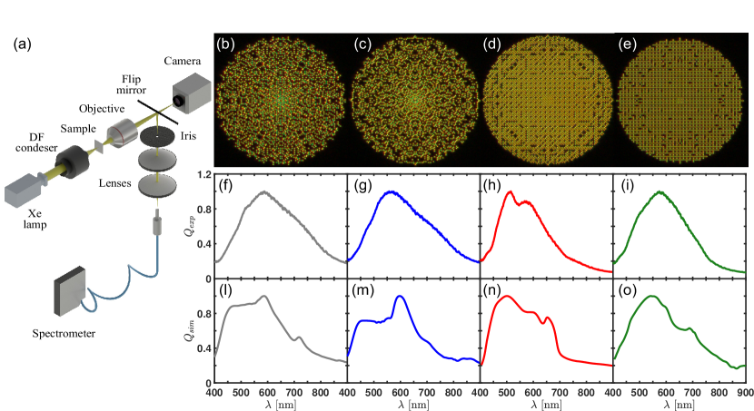
Figure 16: Scattering properties of prime arrays. (a) Experimental setup to perform dark-field microscopy measurements and dark-field scattering spectra. Multispectral dark-field images of Eisenstein (b), Gaussian (c), Hurwitz (d), and Lifschitz (e) prime arrays. Measured (f-i) dark-field scattering spectra and calculated (l-o) scattering efficiencies of the corresponding array at the top of each column.

When the prime arrays are illuminated by a white light source, they give rise to highly organized structural color patterns as shown in Fig. 16 (b-e). The formation of these multispectral complex patterns, especially in the Eisenstein and Gaussian configurations, is the result of a redistribution of the incident radiation field intensity, at each given wavelength, into a multitude of spatial directions. These spatial colorimetric patterns are, therefore, the result of the complex superposition of the scattered fields that strongly depend on the nature of the optical modes generated by the interaction of light with the multifractal geometrical support of these arrays. Interestingly, these unique features were employed in the engineer of optical devices, based on Gaussian prime distributions, where both the spectral and spatial information encoded in the scattered fields were retrieved for efficient detection of protein monolayers Lee et al. (2010).

Fig. 16 (f-i) show the measured normalized scattering intensity of prime arrays. These spectra reveal variations of the array scattering intensity as a function of the incident wavelength. Specifically, all the structures display a broad spectrum in the range (500 nm,650 nm) except for the Hurwitz in which two clear peaks are visible. These scattering peaks are dominated by the electric and magnetic dipole terms of the multipolar expansions Mulholland et al. (1994); Dal Negro et al. (2019). Moreover, the spectral mixing of dipolar modes makes these arrays relatively insensitive to increasing the average interparticle separation. The absence of a red-shift of the scattering band as a function of interparticle separation, related to the coherent contribution of radiative coupling Trevino et al. (2011), is consistent with the inhomogeneity and the multifractal complexity of their geometrical supports.

To support the interpretation of our experimental results, we have evaluate the scattering efficiencies (the ratio of the scattering cross section to the volume of the particles) of prime arrays by employing the EMCDA approximation. These results, reported in Fig. 16 (l-o), are evaluated as the difference of the extinction and the absorption efficiency, $i.e.$ $Q_{sca}=Q_{ext}-Q_{abs}$ Dal Negro et al. (2019). The simulated prime arrays are characterized by more than 2000 nanospheres of 105 nm in radius separated by an average center-to-center separation of 450 nm embedded in an effective refractive index medium to emulate the presence of a quartz substrate. These results, which approximate the nanocylinder shapes using spherical particles of 105 nm radius, are sufficiently well-described by taking into account only the electric and magnetic dipole terms, while the contribution of higher order electromagnetic multipoles can be safely neglected for incident wavelength larger than $\sim$470 nm. To match the experimental conditions, we have used unpolarized excitation and we have performed an average over three different angles of incidence ($\theta_{inc}$=50^∘,55^∘,65^∘-consistent with our experimental conditions). Fig. 16 (l-o) reproduce qualitatively the main features of the measured scattering spectra of prime arrays. The discrepancy between simulation and experiment is attributed to the combined effects of the non-collinear nature of the dark-field excitation (limiting frequency resolution) and to the non-spherical shape of the fabricated nanocylinders.

References

- Mandelbrot (1983) B. B. Mandelbrot, The fractal geometry of nature, Vol. 173 (W.H. freeman New York, 1983).
- Berry (1979) M. Berry, Diffractals, J. Phys. A 12, 781 (1979).
- Soljačić et al. (2000) M. Soljačić, M. Segev, and C. R. Menyuk, Self-similarity and fractals in soliton-supporting systems, Phys. Rev. E 61, R1048 (2000).
- Ilday et al. (2004) F. Ilday, J. Buckley, W. Clark, and F. Wise, Self-similar evolution of parabolic pulses in a laser, Phys. Rev. Lett. 92, 213902 (2004).
- Cao and Wiersig (2015) H. Cao and J. Wiersig, Dielectric microcavities: Model systems for wave chaos and non-Hermitian physics, Rev. Mod. Phys. 87, 61 (2015).
- Bandres et al. (2016) M. A. Bandres, M. C. Rechtsman, and M. Segev, Topological photonic quasicrystals: Fractal topological spectrum and protected transport, Phys. Rev. X 6, 011016 (2016).
- Aslan et al. (2016) E. Aslan, E. Aslan, R. Wang, M. K. Hong, S. Erramilli, M. Turkmen, O. G. Saracoglu, and L. Dal Negro, Multispectral Cesaro-Type Fractal Plasmonic Nanoantennas, ACS Photonics 3, 2102 (2016).
- Joannopoulos et al. (1997) J. D. Joannopoulos, P. R. Villeneuve, and S. Fan, Photonic crystals: putting a new twist on light, Nature 386, 143 (1997).
- Wiersma (2013) D. S. Wiersma, Disordered photonics, Nat. Photonics 7, 188 (2013).
- Lagendijk et al. (2009) A. Lagendijk, B. Van Tiggelen, and D. S. Wiersma, Fifty years of Anderson localization, Phys. Today 62, 24 (2009).
- Vardeny et al. (2013) Z. V. Vardeny, A. Nahata, and A. Agrawal, Optics of photonic quasicrystals, Nat. Photonics 7, 177 (2013).
- Dal Negro and Boriskina (2012) L. Dal Negro and S. V. Boriskina, Deterministic aperiodic nanostructures for photonics and plasmonics applications, Laser Photonics Rev. 6, 178 (2012).
- Torquato (2018) S. Torquato, Hyperuniform states of matter, Phys. Rep. 745, 1 (2018).
- Segev et al. (2013) M. Segev, Y. Silberberg, and D. N. Christodoulides, Anderson localization of light, Nat. Photonics 7, 197 (2013).
- Shalaev (2007) V. M. Shalaev, Optical negative-index metamaterials, Nat. Photonics 1, 41 (2007).
- Kabashin et al. (2009) A. Kabashin, P. Evans, S. Pastkovsky, W. Hendren, G. Wurtz, R. Atkinson, R. Pollard, V. Podolskiy, and A. Zayats, Plasmonic nanorod metamaterials for biosensing, Nat. Mater. 8, 867 (2009).
- Zheludev and Kivshar (2012) N. I. Zheludev and Y. S. Kivshar, From metamaterials to metadevices, Nat. Mater. 11, 917 (2012).
- Khajetoorians et al. (2019) A. A. Khajetoorians, D. Wegner, A. F. Otte, and I. Swart, Creating designer quantum states of matter atom-by-atom, Nature Reviews Physics , 1 (2019).
- Bloch et al. (2012) I. Bloch, J. Dalibard, and S. Nascimbene, Quantum simulations with ultracold quantum gases, Nat. Phys. 8, 267 (2012).
- Stanley and Meakin (1988) H. E. Stanley and P. Meakin, Multifractal phenomena in physics and chemistry, Nature 335, 405 (1988).
- Chhabra and Jensen (1989) A. Chhabra and R. V. Jensen, Direct determination of the f() singularity spectrum, Phys. Rev. Lett. 62, 1327 (1989).
- Frisch and Parisi (1980) U. Frisch and G. Parisi, Fully developed turbulence and intermittency, Ann. N. Y. Acad. Sci. 357, 359 (1980).
- Richardella et al. (2010) A. Richardella, P. Roushan, S. Mack, B. Zhou, D. A. Huse, D. D. Awschalom, and A. Yazdani, Visualizing critical correlations near the metal-insulator transition in Ga1-xMnxAs, Science 327, 665 (2010).
- Evers and Mirlin (2008) F. Evers and A. D. Mirlin, Anderson transitions, Rev. Mod. Phys. 80, 1355 (2008).
- Zhao et al. (2019) K. Zhao, H. Lin, X. Xiao, W. Huang, W. Yao, M. Yan, Y. Xing, Q. Zhang, Z.-X. Li, S. Hoshino, J. Wang, S. Zhou, L. Gu, M. Saeed Bahramy, H. Yao, N. Nagaosa, Q.-K. Xue, K. T. Law, X. Chen, and S.-H. Ji, Disorder-induced multifractal superconductivity in monolayer niobium dichalcogenides, Nat. Phys. 15, 904 (2019).
- Chabé et al. (2008) J. Chabé, G. Lemarié, B. Grémaud, D. Delande, P. Szriftgiser, and J. C. Garreau, Experimental observation of the Anderson metal-insulator transition with atomic matter waves, Phys. Rev. Lett. 101, 255702 (2008).
- Desideri et al. (1989) J.-P. Desideri, L. Macon, and D. Sornette, Observation of critical modes in quasiperiodic systems, Phys. Rev. Lett. 63, 390 (1989).
- Faez et al. (2009) S. Faez, A. Strybulevych, J. H. Page, A. Lagendijk, and B. A. van Tiggelen, Observation of multifractality in Anderson localization of ultrasound, Phys. Rev. Lett. 103, 155703 (2009).
- Maciá (2005) E. Maciá, The role of aperiodic order in science and technology, Rep. Prog. Phys. 69, 397 (2005).
- Lang (1994) S. Lang, Algebraic Number Theory, 2nd edition (Springer, NY, 1994).
- Dekker (1994) T. J. Dekker, Primes in quadratic fields, Quarterly 7, 357 (1994).
- Conway and Smith (2003) J. H. Conway and D. A. Smith, On quaternions and octonions (AK Peters/CRC Press, Boca Raton, 2003).
- Wang et al. (2018a) R. Wang, F. A. Pinheiro, and L. Dal Negro, Spectral statistics and scattering resonances of complex primes arrays, Phys. Rev. B 97, 024202 (2018a).
- Baake and Grimm (2013) M. Baake and U. Grimm, Aperiodic order, Vol. 1 (Cambridge University Press, 2013).
- Riboli et al. (2017) F. Riboli, F. Uccheddu, G. Monaco, N. Caselli, F. Intonti, M. Gurioli, and S. Skipetrov, Tailoring correlations of the local density of states in disordered photonic materials, Phys. Rev. Lett. 119, 043902 (2017).
- Oliver and Soundararajan (2016) R. J. L. Oliver and K. Soundararajan, Unexpected biases in the distribution of consecutive primes, Proc. Natl. Acad. Sci. U.S.A. 113, E4446 (2016).
- Wolf (1989) M. Wolf, Multifractality of prime numbers, Physica 160, 24 (1989).
- Viebahn et al. (2019) K. Viebahn, M. Sbroscia, E. Carter, J.-C. Yu, and U. Schneider, Matter-wave diffraction from a quasicrystalline optical lattice, Phys. Rev. Lett. 122, 110404 (2019).
- Zheng et al. (2014) J. Zheng, S. Bao, Y. Guo, and P. Jin, TiO2 films prepared by DC reactive magnetron sputtering at room temperature: Phase control and photocatalytic properties, Surf. Coat. Tech. 240, 293 (2014).
- Schneider et al. (2012) C. A. Schneider, W. S. Rasband, and K. W. Eliceiri, NIH Image to ImageJ: 25 years of image analysis, Nat. Methods 9, 671 (2012).
- Vardi (1998) I. Vardi, Prime percolation, Experimental Mathematics 7, 275 (1998).
- Rudnick and Waxman (2019) Z. Rudnick and E. Waxman, Angles of Gaussian primes, Israel Journal of Mathematics 232, 159 (2019).
- Prasad (2014) S. Prasad, Walks on Primes in Imaginary Quadratic Fields, arXiv preprint arXiv:1412.2310 (2014).
- Hentschel and Procaccia (1983) H. Hentschel and I. Procaccia, The infinite number of generalized dimensions of fractals and strange attractors, Physica D 8, 435 (1983).
- Halsey et al. (1986) T. C. Halsey, P. Meakin, and I. Procaccia, Scaling structure of the surface layer of diffusion-limited aggregates, Phys. Rev. Lett. 56, 854 (1986).
- Meakin et al. (1985) P. Meakin, H. E. Stanley, A. Coniglio, and T. A. Witten, Surfaces, interfaces, and screening of fractal structures, Phys. Rev. A 32, 2364 (1985).
- Hilborn et al. (2000) R. C. Hilborn et al., Chaos and nonlinear dynamics: an introduction for scientists and engineers (Oxford University Press on Demand, 2000).
- Nakayama and Yakubo (2013) T. Nakayama and K. Yakubo, Fractal concepts in condensed matter physics, Vol. 140 (Springer Science & Business Media, 2013).
- Feder (2013) J. Feder, Fractals (Springer Science & Business Media, 2013).
- Muzy et al. (1994) J.-F. Muzy, E. Bacry, and A. Arneodo, The multifractal formalism revisited with wavelets, Int. J. Bifurc. Chaos Appl. Sci. 4, 245 (1994).
- Mandelbrot et al. (1997) B. B. Mandelbrot, A. J. Fisher, and L. E. Calvet, A multifractal model of asset returns, Cowles Foundation Discussion Paper (1997).
- Schmitt et al. (2000) F. Schmitt, D. Schertzer, and S. Lovejoy, Multifractal fluctuations in finance, IJTAF 3, 361 (2000).
- Schertzer et al. (1997) D. Schertzer, S. Lovejoy, F. Schmitt, Y. Chigirinskaya, and D. Marsan, Multifractal cascade dynamics and turbulent intermittency, Fractals 5, 427 (1997).
- Riedi et al. (1999) R. H. Riedi, M. S. Crouse, V. J. Ribeiro, and R. G. Baraniuk, A multifractal wavelet model with application to network traffic, IEEE T. Inform. Theory 45, 992 (1999).
- Taqqu et al. (1997) M. S. Taqqu, V. Teverovsky, and W. Willinger, Is network traffic self-similar or multifractal? Fractals 5, 63 (1997).
- Ribeiro et al. (2000) V. J. Ribeiro, M. J. Coates, R. H. Riedi, S. Sarvotham, B. Hendricks, and R. G. Baraniuk, Multifractal cross-traffic estimation, in ITC Conference on IP Traffic, Modeling and Management (2000).
- Albuquerque and Cottam (2003) E. L. Albuquerque and M. G. Cottam, Theory of elementary excitations in quasiperiodic structures, Phys. Rep 376, 225 (2003).
- Trevino et al. (2012) J. Trevino, S. F. Liew, H. Noh, H. Cao, and L. Dal Negro, Geometrical structure, multifractal spectra and localized optical modes of aperiodic Vogel spirals, Opt. Express 20, 3015 (2012).
- Maciá (1999) E. Maciá, Physical nature of critical modes in Fibonacci quasicrystals, Phys. Rev. B 60, 10032 (1999).
- Ryu et al. (1992) C. Ryu, G. Oh, and M. Lee, Extended and critical wave functions in a Thue–Morse chain, Phys. Rev. B 46, 5162 (1992).
- Sorensen (2001) C. Sorensen, Light scattering by fractal aggregates: a review, Aerosol Sci. Tech.. 35, 648 (2001).
- Sroor et al. (2019) H. Sroor, D. Naidoo, S. W. Miller, J. Nelson, J. Courtial, and A. Forbes, Fractal light from lasers, Phys. Rev. A 99, 013848 (2019).
- Rodriguez et al. (2009) A. Rodriguez, L. J. Vasquez, and R. A. Römer, Multifractal analysis with the probability density function at the three-dimensional Anderson transition, Phys. Rev. Lett. 102, 106406 (2009).
- Schreiber and Grussbach (1991) M. Schreiber and H. Grussbach, Multifractal wave functions at the Anderson transition, Phys. Rev. Lett. 67, 607 (1991).
- Stanley (1971) H. E. Stanley, Phase transitions and critical phenomena (Clarendon Press, Oxford, 1971).
- Kempkes et al. (2019) S. Kempkes, M. Slot, S. Freeney, S. Zevenhuizen, D. Vanmaekelbergh, I. Swart, and C. M. Smith, Design and characterization of electrons in a fractal geometry, ?Nat. Phys.. 15, 127 (2019).
- Baake and Grimm (2008) M. Baake and U. Grimm, The singular continuous diffraction measure of the Thue–Morse chain, J. Journal of Physics A 41, 422001 (2008).
- Wang et al. (2018b) R. Wang, M. Röntgen, C. V. Morfonios, F. A. Pinheiro, P. Schmelcher, and L. Dal Negro, Edge modes of scattering chains with aperiodic order, Opt. Lett. 43, 1986 (2018b).
- Rusek et al. (2000) M. Rusek, J. Mostowski, and A. Orłowski, Random Green matrices: From proximity resonances to Anderson localization, Phys. Rev. A 61, 022704 (2000).
- Dal Negro et al. (2019) L. Dal Negro, Y. Chen, and F. Sgrignuoli, Aperiodic photonics of elliptic curves, Crystals 9, 482 (2019).
- Yurkin and Hoekstra (2007) M. A. Yurkin and A. G. Hoekstra, The discrete dipole approximation: an overview and recent developments, J Quant Spectrosc. Ra. 106, 558 (2007).
- Doyle (1989) W. T. Doyle, Optical properties of a suspension of metal spheres, Phys. Rev. B 39, 9852 (1989).
- Mulholland et al. (1994) G. W. Mulholland, C. F. Bohren, and K. A. Fuller, Light scattering by agglomerates: coupled electric and magnetic dipole method, Langmuir 10, 2533 (1994).
- Skipetrov (2019) S. E. Skipetrov, Finite-size scaling of the density of states inside band gaps of ideal and disordered photonic crystals, arXiv preprint arXiv:1909.13661 (2019).
- Rusek et al. (1996) M. Rusek, A. Orłowski, and J. Mostowski, Localization of light in three-dimensional random dielectric media, Phys. Rev. E 53, 4122 (1996).
- Lagendijk and Van Tiggelen (1996) A. Lagendijk and B. A. Van Tiggelen, Resonant multiple scattering of light, Phys. Rep 270, 143 (1996).
- Skipetrov and Sokolov (2014) S. E. Skipetrov and I. M. Sokolov, Absence of Anderson localization of light in a random ensemble of point scatterers, Phys. Rev. Lett. 112, 023905 (2014).
- Sgrignuoli et al. (2019a) F. Sgrignuoli, R. Wang, F. Pinheiro, and L. Dal Negro, Localization of scattering resonances in aperiodic Vogel spirals, Phys. Rev. B 99, 104202 (2019a).
- Sgrignuoli et al. (2019b) F. Sgrignuoli, M. Röntgen, C. V. Morfonios, P. Schmelcher, and L. Dal Negro, Compact localized states of open scattering media: a graph decomposition approach for an ab initio design, Opt. Lett. 44, 375 (2019b).
- Sgrignuoli et al. (2015) F. Sgrignuoli, G. Mazzamuto, N. Caselli, F. Intonti, F. S. Cataliotti, M. Gurioli, and C. Toninelli, Necklace state hallmark in disordered 2D photonic systems, ACS Photonics 2, 1636 (2015).
- Yasumoto (2005) K. Yasumoto, Electromagnetic theory and applications for photonic crystals (CRC press, 2005).
- Grassberger and Procaccia (1983) P. Grassberger and I. Procaccia, Characterization of strange attractors, Phys. Rev. Lett. 50, 346 (1983).
- Mandelbrot (1977) B. B. Mandelbrot, Fractals: form, chance, and dimension, Vol. 706 (WH Freeman San Francisco, 1977).
- Voss (1988) R. F. Voss, Fractals in nature: from characterization to simulation, in The science of fractal images (Springer, 1988) pp. 21–70.
- Gouyet (1996) J.-F. Gouyet, Physics and fractal structures (Springer Verlag, 1996).
- Korvin (1992) G. Korvin, Fractal models in the earth sciences, Vol. 448 (elsevier Amsterdam, 1992).
- Wegner (1980) F. Wegner, Inverse participation ratio in 2+ dimensions, Zeitschrift für Physik B Condensed Matter 36, 209 (1980).
- Aoki (1983) H. Aoki, Critical behaviour of extended states in disordered systems, J. Phys. Condens. Matter 16, L205 (1983).
- Castellani and Peliti (1986) C. Castellani and L. Peliti, Multifractal wavefunction at the localisation threshold, J. Phys. A 19, L429 (1986).
- Ioffe et al. (1985) L. Ioffe, I. Sagdeev, and V. Vinokur, A large dispersion of physical quantities as a consequence of Anderson localisation, J. Phys. C 18, L641 (1985).
- Lee et al. (2010) S. Y. Lee, J. J. Amsden, S. V. Boriskina, A. Gopinath, A. Mitropolous, D. L. Kaplan, F. G. Omenetto, and L. Dal Negro, Spatial and spectral detection of protein monolayers with deterministic aperiodic arrays of metal nanoparticles, Proc. Natl. Acad. Sci. U.S.A. 107, 12086 (2010).
- Trevino et al. (2011) J. Trevino, H. Cao, and L. Dal Negro, Circularly symmetric light scattering from nanoplasmonic spirals, Nano Lett. 11, 2008 (2011).