Sparse Interpolation in Terms of Multivariate Chebyshev Polynomials

Abstract

Sparse interpolation refers to the exact recovery of a function as a short linear combination of basis functions from a limited number of evaluations. For multivariate functions, the case of the monomial basis is well studied, as is now the basis of exponential functions. Beyond the multivariate Chebyshev polynomial obtained as tensor products of univariate Chebyshev polynomials, the theory of root systems allows to define a variety of generalized multivariate Chebyshev polynomials that have connections to topics such as Fourier analysis and representations of Lie algebras. We present a deterministic algorithm to recover a function that is the linear combination of at most $r$ such polynomials from the knowledge of $r$ and an explicitly bounded number of evaluations of this function.
Keywords: Chebyshev Polynomials, Hankel matrix, root systems, sparse interpolation, Weyl groups.
Mathematics Subject Classification: 13A50, 17B10, 17B22, 30E05, 33C52, 33F10, 68W30

1 Introduction

The goal of sparse interpolation is the exact recovery of a function as a short linear combination of elements in a specific set of functions, usually of infinite cardinality, from a limited number of evaluations, or other functional values. The function to recover is sometimes refered to as a blackbox: it can be evaluated, but its expression is unknown. We consider the case of a multivariate function $f(x_{1},\ldots,x_{n})$ that is a sum of generalized Chebyshev polynomials and present an algorithm to retrieve the summands. We assume we know the number of summands, or an upper bound for this number, and the values of the function at a finite set of well chosen points.

Beside their strong impact in analysis, Chebyshev polynomials arise in the representation theory of simple Lie algebras. In particular, the Chebyshev polynomials of the first kind may be identified with orbit sums of weights of the Lie algebra $\mathrm{sl}_{2}$ and the Chebyshev polynomials of the second kind may be identified with characters of this Lie algebra. Both types of polynomials are invariant under the action of the symmetric group $\{1,-1\}$, the associated associated Weyl group, on the exponents of the monomials. In presentations of the theory of Lie algebras (c.f., [11, Ch.5,§3]), this identification is often discussed in the context of the associated root systems and we will take this approach. In particular, we define the generalized Chebyshev polynomials associated to a root system, as similarly done in [27, 41, 43, 46]. Several authors have already exploited the connection between Chebyshev polynomials and the theory of Lie algebras or root systems (e.g., [18], [47], [57]) and successfully used this in the context of quadrature problems [38, 42, 44, 46] or differential equations [53].

A forebear of our algorithm is Prony’s method to retrieve a univariate function as a linear combination of exponential functions from its values at equally spaced points [51]. The method was further developed in a numerical context [48]. In exact computation, mostly over finite fields, some of the algorithms for the sparse interpolation of multivariate polynomial functions in terms of monomials bear similarities to Prony’s method and have connections with linear codes [8, 3]. General frameworks for sparse interpolation were proposed in terms of sums of characters of Abelian groups and sums of eigenfunctions of linear operators [19, 25]. The algorithm in [35] for the recovery of a linear combination of univariate Chebyshev polynomials does not fit in these frameworks though. Yet, as observed in [5], a simple change of variables turns Chebyshev polynomials into Laurent polynomials with a simple symmetry in the exponents. This symmetry is most naturally explained in the context of root systems and Weyl groups and leads to a multivariate generalization.

Previous algorithms [5, 22, 30, 35, 49] for sparse interpolation in terms of Chebyshev polynomials of one variable depend heavily on the relations for the products, an identification property, and the commutation of composition. We show in this paper how analogous results hold for generalized Chebyshev polynomials of several variables and stem from the underlying root system. As already known, expressing the multiplication of generalized Chebyshev polynomials in terms of other generalized Chebyshev polynomials is presided over by the Weyl group. As a first original result we show how to select $n$ points in $\mathbb{Q}^{n}$ so that each $n$-variable generalized Chebyshev polynomial is determined by its values at these $n$ points (Lemma 2.25, Theorem 2.27). A second original observation permits to generalize the commutation property in that we identify points where commutation is available (Proposition 3.4).

To provide a full algorithm, we revisit sparse interpolation in an intrinsically multivariate approach that allows one to preserve and exploit symmetry. For the interpolation of sparse sums of Laurent monomials the algorithm presented (Section 3.1) has strong ties with a multivariate Prony method [34, 45, 55]. It associates to each sum of $r$ monomials $f(x)=\sum_{\alpha}a_{\alpha}x^{\alpha},\mbox{ where }x^{\alpha}=x_{1}^{\alpha_{1}}\ldots x_{n}^{\alpha_{n}}$ and $a_{\alpha}$ in a field $\mathbb{K}$, a linear form $\Omega:\mathbb{K}[x,x^{-1}]\rightarrow\mathbb{K}$ given by $\Omega(p)=\sum_{\alpha}a_{\alpha}p(\zeta_{\alpha})$ where $\zeta_{\alpha}=(\xi^{\alpha_{1}},\ldots,\xi^{\alpha_{n}})$ for suitable $\xi$. This linear form allows us to define a Hankel operator from $K[x,x^{-1}]$ to its dual (see Section 4.1) whose kernel is an ideal $I$ having precisely the $\zeta_{\alpha}$ as its zeroes. The $\zeta_{\alpha}$ can be recovered as eigenvalues of multiplication maps on $\mathbb{K}[x,x^{-1}]/I$. The matrices of these multiplication maps can actually be calculated directly in terms of the matrices of a Hankel operator, without explicitly calculating $I$. One can then find the $\zeta_{\alpha}$ and the $a_{\alpha}$ using only linear algebra and evaluation of the original polynomial $f(x)$ at well-chosen points. The calculation of the $(\alpha_{1},\ldots,\alpha_{n})$ is then reduced to the calculation of logarithms.

The usual Hankel or mixed Hankel-Toepliz matrices that appeared in the literature on sparse interpolation [8, 35] are actually the matrices of the Hankel operator mentioned above in the different univariate polynomial bases considered. The recovery of the support of a linear form with this type of technique also appears in optimization, tensor decomposition and cubature [2, 9, 13, 15, 36, 37]. We present new developments to take advantage of the invariance or semi-invariance of the linear form. This allows us to reduce the size of the matrices involved by a factor equal to the order of the Weyl group (Section 4.3).

For sparse interpolation in terms of Chebyshev polynomials (Section 3.2 and 3.3), one again recasts this problem in terms of a linear form on a Laurent polynomial ring. We define an action of the Weyl group on this ring as well as on the underlying ambient space and note that the linear form is invariant or semi-invariant according to whether we consider generalized Chebyshev polynomials of the first or second kind. Evaluations, at specific points, of the function to interpolate provide the knowledge of the linear form on a linear basis of the invariant subring or semi-invariant module. In the case of interpolation of sparse sums of Laurent monomials the seemingly trivial yet important fact that $(\xi^{\beta})^{\alpha}=(\xi^{\alpha})^{\beta}$ is crucial to the algorithm. In the multivariate Chebyshev case we identify a family of evaluation points that provides a similar commutation property in the Chebyshev polynomials (Lemma 3.4).

Since the linear form is invariant, or semi-invariant, the support consists of points grouped into orbits of the action of the Weyl group. Using tools developed in analogy to the Hankel formulation above, we show how to recover the values of the fundamental invariants (Algorithm 4.15) on each of these orbits and, from these, the values of the Chebyshev polynomials that appear in the sparse sum. Furthermore, we show how to recover each Chebyshev polynomial from its values at $n$ carefully selected points (Theorem 2.27).

The relative cost of our algorithms depends on the linear algebra operations used in recovering the support of the linear form and the number of evaluations needed. Recovering the support of a linear form on the Laurent polynomial ring is solved with linear algebra after introducing the appropriate Hankel operators. Symmetry reduces the size of matrices, as expected, by a factor the order of the group. Concerning evaluations of the function to recover, we need evaluations to determine certain sunbmatrices of maximum rank used in the linear algebra component of the algorithms. To bound the number of evaluations needed, we rely on the interpolation property of sets of polynomials indexed by the hyperbolic cross (Proposition 4.5, Corollary 4.12), a result generalizing the case of monomials in [55]. The impact of this on the relative costs of the algorithms is discussed in Section 3.4.

The paper is organized as follows. In Section 2, we begin by describing the connection between univariate Chebyshev polynomials and the representation theory of traceless $2\times 2$ matrices. We then turn to the multivariate case and review the theory of root systems needed to define and work with generalized Chebyshev polynomials. The section concludes with the first original contribution: we show how an $n$-variable Chebyshev polynomial, of the first or second kind, is determined by its values on $n$ special points. In Section 3 we show how multivariate sparse interpolation can be reduced to retrieving the support of certain linear forms on a Laurent polynomial ring. For sparse interpolation in terms of multivariate Chebyshev polynomials of the first and second kind, we show how we can consider the restriction of the linear form to the ring of invariants of the Weyl group or the module of semi-invariants. In addition, we discuss some of the costs of our algorithm as compared to treating generalized Chebyshev polynomials as sums of monomials. In Section 4 we introduce Hankel operators and their use in determining algorithmically the support of a linear form through linear algebra operations. After reviewing the definitions of Hankel operators and multiplication matrices in the context of linear forms on a Laurent polynomial ring, we extend these tools to apply to linear forms invariant under a Weyl group and show how these developments allow one to scale down the size of the matrices by a factor equal to the order of this group. Throughout these sections we provide examples to illustrate the theory and the algorithms. In Section 5 we discuss the global algorithm and point out some directions of further improvement.

Acknowledgment: The authors wish to thank the Fields institute and the organizers of the thematic program on computer algebra where this research was initiated. They also wish to thank Andrew Arnold for discussions on sparse interpolation and the timely pointer on the use of the hypercross in the multivariate case.

2 Chebyshev polynomials

In this section we first discuss how the usual Chebyshev polynomials arise from considerations concerning root systems and their Weyl group. This approach allows us to give higher dimensional generalizations of these polynomials [27, 46]. We review the results about root systems and representation theory allowing us to define the generalized Chebyshev polynomials of the first and second kind. This section concludes with the first original result in this article necessary to our purpose: we show how one can determine the degree of a Chebyshev polynomial from its values at few well chosen points.

2.1 Univariate Chebyshev polynomials

The univariate Chebyshev polynomials of the first and second kind arise in many contexts; approximation theory, polynomial interpolation, and quadrature formulas are examples. A direct and simple way to define these polynomials is as follows.

Definition 2.1

1. The Chebyshev polynomials of the first kind, $\{\tilde{T}_{n}(x)\ |\ n=0,1,2,\ldots\}$, are the unique monic polynomials satisfying

   $$\tilde{T}_{n}(\cos(\theta))=\cos(n\,\theta)\quad\mbox{ or }\quad\tilde{T}_{n}\left(\frac{x+x^{-1}}{2}\right)=\frac{x^{n}+x^{-n}}{2}.$$

2. The Chebyshev polynomials of the second kind, $\{\tilde{U}_{n}(x)\ |\ n=0,1,2,\ldots\}$, are the unique monic polynomials satisfying

   $$\tilde{U}_{n}(\cos(\theta))=\frac{\sin((n+1)\,\theta)}{\sin(\theta)}\quad\mbox{ or }\quad{\tilde{U}_{n}\left(\frac{x+x^{-1}}{2}\right)=\frac{x^{(n+1)}-x^{-(n+1)}}{x-x^{-1}}=x^{n}+x^{n-2}+\dots+x^{2-n}+x^{-n}}.$$

The second set of equalities for $\tilde{T}_{n}$ and $\tilde{U}_{n}$ are familiar when written in terms of $x=e^{i\theta}$ since $\cos{n\theta}=\frac{1}{2}\left(e^{in\theta}+e^{-in\theta}\right)$ and $\sin(n\theta)=\frac{1}{2}\left(e^{in\theta}-e^{-in\theta}\right)$. We introduced these equalities in terms of $x$ for a clearer connection with the following sections.

These polynomials also arise naturally when one studies the representation theory of the Lie algebra $\mathrm{sl}_{2}(\mathbb{C})$ of $2\times 2$-matrices with zero trace [18, 57]. Any representation $\pi:\mathrm{sl}_{2}(\mathbb{C})\rightarrow\mathrm{gl}_{n}(\mathbb{C})$ is a direct sum of irreducible representations. For each nonnegative integer $n$, there is a unique irreducible representation $\pi_{n}:\mathrm{sl}_{2}(\mathbb{C})\rightarrow\mathrm{gl}_{n+1}(\mathbb{C})$ of dimension $n+1$ (see [56, Capitre IV] for a precise description). Restricting this representation to the diagonal matrices $\left\{\operatorname{diag}(a,-a)\ |\ a\in\mathbb{C}\right\}$, this map is given by $\pi_{n}\left(\operatorname{diag}(a,\;-a)\right)=\operatorname{diag}(na,\;(n-2)\,a,\;\ldots,\;(2-n)\,a,\;-n\,a)$. Each of the maps $\operatorname{diag}(a,\;-a)\mapsto m\,a$, for $m=n,\,n-2,\,\ldots,\,2-n,\,-n$ is called a weight of this representation. The set of weights appearing in the representations of $\mathrm{sl}_{2}(\mathbb{C})$ may therefore be identified with the lattice of integers in the one-dimensional vector space $\mathbb{R}$. The group of automorphisms of this vector space that preserves this lattice is precisely the two element group $\{id,\sigma\}$ where $id(m)=m$ and $\sigma(m)=-m$. This group is called the Weyl group $\mathcal{W}$.

We now make the connection between Lie theory and Chebyshev polynomials. Identify the weight corresponding to the integer $m$ with the weight monomial $x^{m}$ in the Laurent polynomial ring $\mathbb{Z}[x,x^{-1}]$ and let the generator $\sigma$ of the group $\mathcal{W}$ act on this ring via the map $\sigma\cdot x^{m}=x^{\sigma(m)}$. For each weight monomial $x^{m},m\geq 0$, we can define the orbit polynomial

$${\Theta}_{m}(x)=x^{m}+x^{-m}$$

and the character polynomial

$${\Xi}_{m}(x)=x^{m}+x^{m-2}+\ldots+x^{2-m}+x^{-m}.$$

Note that for each $m$, both of these polynomials lie in the ring of invariants $\mathbb{Z}[x,x^{-1}]^{\mathcal{W}}=\mathbb{Z}[x+x^{-1}]$ of the Weyl group. Therefore there exist polynomials ${T}_{n}(X)$ and ${U}_{n}(X)$ such that ${\Theta}_{n}(x)={T}_{n}(x+x^{-1})$ and ${\Xi}_{n}(x)={U}_{n}(x+x^{-1})$. The Chebyshev polynomials of the first and second kind can be recovered using the formulas

$$\tilde{T}_{n}(X)=\frac{1}{2}{T}_{n}(2X)\mbox{ and }\tilde{U}_{n}(X)={U}_{n}(2X).$$

The previous discussion shows how the classical Chebyshev polynomials arise from representation of a semisimple Lie algebra and the action of the Weyl group on a Laurent polynomial ring. As noted above, this discussion could have started just with the associated root system and its Weyl group and weights. This is precisely what we do in Section 2.3 and 2.4 where we define a generalization of these polynomials for any (reduced) root system.

2.2 Root systems and Weyl groups

We review the definition and results on root systems that are needed to define generalized Chebyshev polynomials. These are taken from [11, Chapitre VI],[26, Chapter 8] or [56, Chapitre V] where complete expositions can be found.

Definition 2.2

Let $V$ be a finite dimensional real vector space with an inner product $\langle\cdot\,,\cdot\rangle$ and $\mathrm{R}$ a finite subset of $V$. We say $\mathrm{R}$ is a root system in $V$ if

1. $\mathrm{R}$ spans $V$ and does not contain $0$.

2. If $\rho,\tilde{\rho}\in\mathrm{R}$, then $s_{\rho}(\tilde{\rho})\in\mathrm{R}$, where $s_{\rho}$ is the reflection defined by $\displaystyle s_{\rho}(\gamma)=\gamma-2\frac{\langle\gamma,\rho\rangle}{\langle\rho,\rho\rangle}\rho,\ \ \gamma\in V.$

3. For all $\rho,\tilde{\rho}\in\mathrm{R}$, $\displaystyle 2\frac{\langle\tilde{\rho},\rho\rangle}{\langle\rho,\rho\rangle}\in\mathbb{Z}.$

4. If $\rho\in\mathrm{R}$, and $c\in\mathbb{R}$, then $c\rho\in R$ if and only if $c=\pm 1$.

The definition of $s_{\rho}$ above implies that $\langle s_{\rho}(\mu),s_{\rho}(\nu)\rangle=\langle\mu,\nu\rangle$ for any $\mu,\nu\in V$.

In many texts, a root system is defined only using the first three of the above conditions and the last condition is used to define a reduced root system. All root systems in this paper are reduced so we include this last condition in our definition and dispense with the adjective “reduced”. Furthermore, some texts define a root system without reference to an inner product (c.f. [11, Chapitre VI],[56, Chapitre V]) and only introduce an inner product later in their exposition. The inner product allows one to identify $V$ with its dual $V^{*}$ in a canonical way and this helps us with many computations.

Definition 2.3

The Weyl group $\mathcal{W}$ of a root system $\mathrm{R}$ in $V$ is the subgroup of the orthogonal group, with respect to the inner product $\langle\cdot\,,\cdot\rangle$, generated by the reflections $s_{\rho}$, $\rho\in\mathrm{R}$.

One can find a useful basis of the ambient vector space $V$ sitting inside the set of roots :

Definition 2.4

Let $\mathrm{R}$ be a root system.

1. A subset $\mathrm{B}=\{\rho_{1},\ldots,\rho_{n}\}$ of $\mathrm{R}$ is a base if

   1. $\mathrm{B}$ is a basis of the vector space $V$.

   2. Every root $\mu\in\mathrm{R}$ can be written as $\mu=\alpha_{1}\rho_{1}+\ldots+\alpha_{n}\rho_{n}$ or $\mu=-\alpha_{1}\rho_{1}-\ldots-\alpha_{n}\rho_{n}$ for some $\alpha\in\mathbb{N}^{n}$.

2. If $\mathrm{B}$ is a base, the roots of the form $\mu=\alpha_{1}\rho_{1}+\ldots+\alpha_{n}\rho_{n}$ for some $\alpha\in\mathbb{N}^{n}$ are called the positive roots and the set of positive roots is denoted by $\mathrm{R}^{+}$.

A standard way to show bases exist (c.f. [26, Chapter 8.4],[56, Chapitre V,§8]) is to start by selecting a hyperplane $H$ that does not contain any of the roots and letting $v$ be an element perpendicular to $H$. One defines $R^{\plus}=\{\rho\in\mathrm{R}\ |\ \langle v,\rho\rangle>0\}$ and then shows that $\mathrm{B}=\{\rho\in\mathrm{R}^{\plus}\ |\ \rho\neq\rho^{\prime}+\rho^{\prime\prime}\mbox{ for any pair }\rho^{\prime},\rho^{\prime\prime}\in\mathrm{R}^{\plus}\}$, the indecomposable positive roots, forms a base. For any two bases $\mathrm{B}$ and $\mathrm{B}^{\prime}$ there exists a $\sigma\in\mathcal{W}$ such that $\sigma(\mathrm{B})=\mathrm{B}^{\prime}$. We fix once and for all a base $\mathrm{B}$ of $\mathrm{R}$.

The base can be used to define the following important cone in $V$.

Definition 2.5

The closed fundamental Weyl chamber in $V$ relative to the base $\mathrm{B}=\{\rho_{1},\ldots,\rho_{n}\}$ is $\Lambda\!\!\Lambda=\{v\in V\ |\ \langle v,\rho_{i}\rangle\geq 0\}$. The interior of $\Lambda\!\!\Lambda$ is called the open fundamental Weyl chamber.

Of course, different bases have different open fundamental Weyl chambers. If $L_{i}$ is the hyperplane perpendicular to an element $\rho_{i}$ in the base $\mathrm{B}$, then the connected components of $V-\bigcup_{i=1}^{n}L_{i}$ correspond to the possible open fundamental Weyl chambers. Furthermore, the Weyl group acts transitively on these components.

The element

$$\rho^{\vee}=2\frac{\rho}{\langle\rho,\rho\rangle}$$

that appears in the definition of $s_{\rho}$ is called the coroot of $\rho$. The set of all coroots is denoted by $\mathrm{R}^{\vee}$ and this set is again a root system called the dual root system with the same Weyl group as $\mathrm{R}$ [11, Chapitre VI, §1.1],[26, Proposition 8.11]. If $\mathrm{B}$ is a base of $\mathrm{R}$ then $\mathrm{B}^{\vee}$ is a base of $\mathrm{R}^{\vee}$.

A root system defines the following lattice in $V$, called the lattice of weights. This lattice and related concepts play an important role in the representation theory of semisimple Lie algebras.

Definition 2.6

Let $\mathrm{B}=\{\rho_{1},\ldots,\rho_{n}\}$ the base of $\mathrm{R}$ and $\mathrm{B}^{\vee}=\{\rho_{1}^{\vee},\ldots,\rho_{n}^{\vee}\}$ its dual.

1. An element $\mu$ of $V$ is called a weight if

   $$\langle\mu,\rho_{i}^{\vee}\rangle=2\frac{\langle\mu,\rho_{i}\rangle}{\langle\rho_{i},\rho_{i}\rangle}\in\mathbb{Z}$$

   for $i=1,\ldots,n$. The set of weights forms a lattice called the weight lattice $\Lambda$.

2. The fundamental weights are elements $\{\omega_{1},\ldots,\omega_{n}\}$ such that $\langle\omega_{i},\rho_{j}^{\vee}\rangle=\delta_{i,j},i,j=1,\ldots,n$.

3. A weight $\mu$ is strongly dominant if $\langle\mu,\rho_{i}\rangle>0$ for all $\rho_{i}\in\mathrm{B}$. A weight $\mu$ is dominant if $\langle\mu,\rho_{i}\rangle\geq 0$ for all $\rho_{i}\in\mathrm{B}$, i.e., $\mu\in\Lambda\!\!\Lambda$.

Weights are occasionally referred to as integral elements, [26, Chapter 8.7]. In describing the properties of their lattice it is useful to first define the following partial order on elements of $V$ [29, Chapter 10.1].

Definition 2.7

For $v_{1},v_{2}\in V$, we define $v_{1}\succ v_{2}$ if $v_{1}-v_{2}$ is a sum of positive roots or $v_{1}=v_{2}$, that is, $v_{1}-v_{2}=\sum_{i=1}^{n}n_{i}\rho_{i}$ for some $n_{i}\in\mathbb{N}$.

The following proposition states three key properties of weights and of dominant weights which we will use later.

Proposition 2.8

1. The weight lattice $\Lambda$ is invariant under the action of the Weyl group $\mathcal{W}$.

2. Let $\mathrm{B}=\{\rho_{1},\ldots,\rho_{n}\}$ be a base. If $\mu$ is a dominant weight and $\sigma\in\mathcal{W}$, then $\mu\succ\sigma(\mu)$. If $\mu$ is a strongly dominant weight, then $\sigma(\mu)=\mu$ if and only if $\sigma$ is the identity.

3. $\displaystyle\delta=\frac{1}{2}\sum_{\rho\in\mathrm{R}^{+}}\rho$ is a strongly dominant weight equal to $\displaystyle\sum_{i=1}^{n}\omega_{i}$.

4. If $\mu_{1}$ and $\mu_{2}$ are dominant weights, then $\langle\mu_{1},\mu_{2}\rangle\geq 0$.

Proof.

The proofs of items 1., 2., and 3. may be found in [29, Section 13.2 and 13.3]. For item 4. it is enough to show this when $\mu_{1}$ and $\mu_{2}$ are fundamental weights since dominant weights are nonnegative integer combinations of these. The fact for fundamental weights follows from Lemma 10.1 and Exercise 7 of Section 13 of [29] (see also [26, Proposition 8.13, Lemma 8.14]).    $\Box$

Example 2.9

The (reduced) root systems have been classified and presentations of these can be found in many texts. We give three examples, $\mathcal{A}_{1},\mathcal{A}_{2},\mathcal{B}_{2}$, here. In most texts, these examples are given so that the inner product is the usual inner product on Euclidean space. We have chosen the following representations because we want the associated weight lattices (defined below) to be the integer lattices in the ambient vector spaces. Nonetheless there is an isomorphism of the underlying inner product spaces identifying these representations.

$\mathcal{A}_{1}$.

This system has two elements $[2],[-2]$ in $V=\mathbb{R}^{1}$. The inner product given by $\langle u,v\rangle=\frac{1}{2}uv$. A base is given by $\rho_{1}=[2]$. The Weyl group has two elements, given by the matrices $\begin{bmatrix}1\end{bmatrix}$ and $\begin{bmatrix}-1\end{bmatrix}$.

$\mathcal{A}_{2}$.

This system has 6 elements $\pm{\begin{bmatrix}2&-1\end{bmatrix}}^{{\mathsf{T}}}$, $\pm{\begin{bmatrix}-1&2\end{bmatrix}}^{{\mathsf{T}}}$, $\pm{\begin{bmatrix}1&1\end{bmatrix}}^{{\mathsf{T}}}\in\mathbb{R}^{2}$ when the inner product is given by $\langle u,v\rangle={u}^{{\mathsf{T}}}S\,v$ where

$$S=\frac{1}{3}\begin{bmatrix}2&1\\ 1&2\end{bmatrix}.$$

A base is given by $\rho_{1}={\begin{bmatrix}2&-1\end{bmatrix}}^{{\mathsf{T}}}$ and $\rho_{2}={\begin{bmatrix}-1&2\end{bmatrix}}^{{\mathsf{T}}}$. We have $\langle\rho_{i},\rho_{i}\rangle=2$ so that $\rho_{i}^{\vee}=\rho_{i}$ for $i=\{1,2\}$.

The Weyl group is of order $6$ and represented by the matrices

$$\underbrace{\left[\begin{array}[]{cc}-1&0\\ \vskip 6.0pt plus 2.0pt minus 2.0pt\cr 1&1\end{array}\right]}_{A_{1}},\;\underbrace{\left[\begin{array}[]{cc}1&1\\ \vskip 6.0pt plus 2.0pt minus 2.0pt\cr 0&-1\end{array}\right]}_{A_{2}},\;\left[\begin{array}[]{cc}0&-1\\ \vskip 6.0pt plus 2.0pt minus 2.0pt\cr-1&0\end{array}\right],\;\left[\begin{array}[]{cc}1&0\\ \vskip 6.0pt plus 2.0pt minus 2.0pt\cr 0&1\end{array}\right],\;\left[\begin{array}[]{cc}-1&-1\\ \vskip 6.0pt plus 2.0pt minus 2.0pt\cr 1&0\end{array}\right],\;\left[\begin{array}[]{cc}0&1\\ \vskip 6.0pt plus 2.0pt minus 2.0pt\cr-1&-1\end{array}\right].$$

where $A_{1}$ and $A_{2}$ are the reflections associated with $\rho_{1}$ and $\rho_{2}$. We implicitly made choices so that the fundamental weights are $\omega_{1}={\begin{bmatrix}1&0\end{bmatrix}}^{{\mathsf{T}}}$ and $\omega_{2}={\begin{bmatrix}0&1\end{bmatrix}}^{{\mathsf{T}}}$. The lattice of weights is thus the integer lattice in $\mathbb{R}^{2}$ and orbits of weights are represented in Figure 2.1.

$\mathcal{B}_{2}$.

This system has 8 elements $\pm{\begin{bmatrix}2&-2\end{bmatrix}}^{{\mathsf{T}}}$, $\pm{\begin{bmatrix}-1&2\end{bmatrix}}^{{\mathsf{T}}}$, $\pm{\begin{bmatrix}0&2\end{bmatrix}}^{{\mathsf{T}}}$, $\pm{\begin{bmatrix}1&0\end{bmatrix}}^{{\mathsf{T}}}$ when the inner product is given by $\langle u,v\rangle={u}^{{\mathsf{T}}}S\,v$ where

$$S=\frac{1}{2}\,\begin{bmatrix}2&1\\ 1&1\end{bmatrix}.$$

A base is given by $\rho_{1}={\begin{bmatrix}2&-2\end{bmatrix}}^{{\mathsf{T}}}$ and $\rho_{2}={\begin{bmatrix}-1&2\end{bmatrix}}^{{\mathsf{T}}}$. We have $\langle\rho_{1},\rho_{1}\rangle=2$ and $\langle\rho_{2},\rho_{2}\rangle=1$. Hence $\rho_{1}^{\vee}=\rho_{1}$ and $\rho_{2}^{\vee}=2\,\rho_{2}$. The Weyl group is of order $8$ and represented by the matrices

$$\left[\begin{array}[]{cc}1&0\\ \vskip 6.0pt plus 2.0pt minus 2.0pt\cr 0&1\end{array}\right],\left[\begin{array}[]{cc}-1&0\\ \vskip 6.0pt plus 2.0pt minus 2.0pt\cr 2&1\end{array}\right],\left[\begin{array}[]{cc}1&1\\ \vskip 6.0pt plus 2.0pt minus 2.0pt\cr 0&-1\end{array}\right],\left[\begin{array}[]{cc}1&1\\ \vskip 6.0pt plus 2.0pt minus 2.0pt\cr-2&-1\end{array}\right],\left[\begin{array}[]{cc}-1&-1\\ \vskip 6.0pt plus 2.0pt minus 2.0pt\cr 2&1\end{array}\right],\left[\begin{array}[]{cc}-1&-1\\ \vskip 6.0pt plus 2.0pt minus 2.0pt\cr 0&1\end{array}\right],\left[\begin{array}[]{cc}1&0\\ \vskip 6.0pt plus 2.0pt minus 2.0pt\cr-2&-1\end{array}\right],\left[\begin{array}[]{cc}-1&0\\ \vskip 6.0pt plus 2.0pt minus 2.0pt\cr 0&-1\end{array}\right].$$

We implicitly made choices so that the fundamental weights are $\omega_{1}={\begin{bmatrix}1&0\end{bmatrix}}^{{\mathsf{T}}}$ and $\omega_{2}={\begin{bmatrix}0&1\end{bmatrix}}^{{\mathsf{T}}}$. The lattice of weights is thus the integer lattice in $\mathbb{R}^{2}$ and orbits of weights are represented in Figure 2.1.

Convention: We will always assume that the root systems are presented in such a way that the associated weight lattices are the integer lattice. This implies that the associated Weyl group lies in $\mathrm{GL}_{n}(\mathbb{Z})$.

We may assume that there is a matrix $S$ with rational entries such that $<v,w>={v}^{{\mathsf{T}}}Sw$. This is not obvious from the definition of a root system but follows from the classification of irreducible root systems. Any root system is the direct sum of orthogonal irreducible root systems ([29, Section 10.4]) and these are isomorphic to root systems given by vectors with rational coordinates where the inner product is the usual inner product on affine space [11, Ch.VI, Planches I-IX]. Taking the direct sum of these inner product spaces one gets an inner product on the ambient space with $S$ having rational entries. For the examples we furthermore choose $S$ so as to have the longest roots to be of norm $2$.

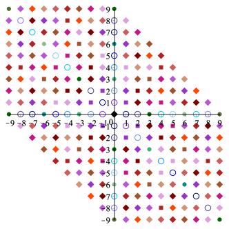
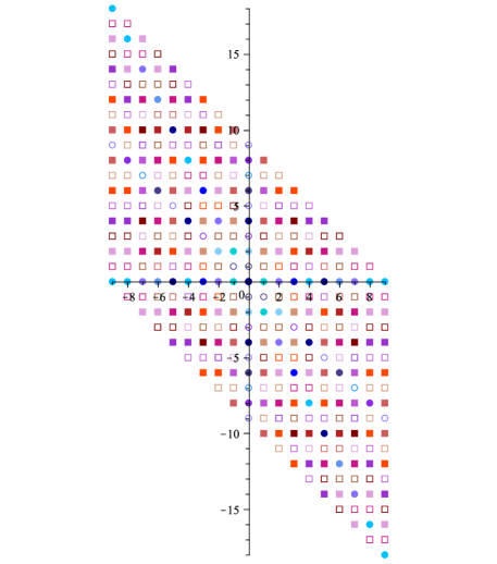
Figure 2.1: $\mathcal{A}_{2}$-orbits and $\mathcal{B}_{2}$-orbits of all $\alpha\in\mathbb{N}^{2}$ with $|\alpha|\leq 9$. Elements of an orbit have the same shape and color. The orbits with $3$, or $4$, elements are represented by circles, the orbits with $6$, or $8$, elements by diamonds or squares. Squares and solid disc symbols are on the sublattice generated by the roots.

2.3 Generalized Chebyshev polynomials of the first kind

As seen in Section 2.1, the usual Chebyshev polynomials can be defined by considering a Weyl group acting on the exponents of monomials in a ring of Laurent polynomials. We shall use this approach to define Chebyshev polynomials of several variables as in [27, 46]. This section defines the generalized Chebyshev polynomials of the first kind. The next section presents how those of the second kind appear in the representations of simple Lie algebras.

Let $\Lambda$ and $\mathcal{W}$ be the weight lattice and the Weyl group associated to a root system. With $\omega_{1},\ldots,\omega_{n}$ the fundamental weights, we identify $\Lambda$ with $\mathbb{Z}^{n}$ through $\omega\rightarrow\alpha={\left[\alpha_{1},\ldots,\alpha_{n}\right]}^{{\mathsf{T}}}$ where $\omega=\alpha_{1}\omega_{1}+\ldots+\alpha_{n}\omega_{n}$.

An arbitrary weight $\omega=\alpha_{1}\omega_{1}+\ldots+\alpha_{n}\omega_{n}\in\Lambda$ is associated with the weight monomial $x^{\alpha}=x_{1}^{\alpha_{1}}\ldots x_{n}^{\alpha_{n}}$. In this way one sees that the group algebra $\mathbb{Z}[\Lambda]$ can be identified with the Laurent polynomial ring $\mathbb{Z}[x_{1},\ldots,x_{n},x_{1}^{-1},\ldots,x_{n}^{-1}]=\mathbb{Z}[x,x^{-1}]$. The action of $\mathcal{W}$ on $\Lambda$ makes us identify $\mathcal{W}$ with subgroup of $\mathrm{GL}_{n}(\mathbb{Z})$.

Let $\mathbb{K}$ be a field of characteristic $0$ and denote $\mathbb{K}\setminus\{0\}$ by $\mathbb{K}^{*}$. The linear action of $\mathcal{W}$ on $\mathbb{K}[x^{\pm}]=\mathbb{K}[x_{1},\,\ldots,\,x_{n},x_{1}^{-1},\,\ldots,\,x_{n}^{-1}]$ is defined by

$$\cdot:\begin{array}[t]{ccc}\mathcal{W}\times\mathbb{K}[x^{\pm}]&\rightarrow&\mathbb{K}[x^{\pm}]\\ \left(A,\,x^{\alpha}\right)&\mapsto&A\cdot x^{\alpha}=x^{A\,\alpha}.\end{array}.$$ (2.1)

We have $(A\cdot f)(x)=f\left(x^{A}\right)$. One can see the above action on $\mathbb{K}[x^{\pm}]$ as induced by the (nonlinear) action on $({\mathbb{K}}^{*})^{n}$ defined by the monomial maps:

$$\begin{array}[t]{ccl}\mathcal{W}\times({\mathbb{K}}^{*})^{n}&\rightarrow&({\mathbb{K}}^{*})^{n}\\ \left(A,\,\zeta\right)&\mapsto&A\star\zeta=\left[\zeta_{1},\,\ldots,\,\zeta_{n}\right]^{A^{-1}}=\left[\zeta^{A^{-1}_{\cdot 1}},\,\ldots,\,\zeta^{A^{-1}_{\cdot n}}\right]\end{array}$$ (2.2)

where $A^{-1}_{\cdot i}$ is the $i$-th column vector of $A^{-1}$. Such actions are sometimes called multiplicative actions [39, Section 3].

For a group morphism $\chi:\mathcal{W}\rightarrow\mathbb{C}^{*}$, $\alpha,\beta\in\mathbb{Z}^{n}$ we define

$${\Psi}^{\chi}_{\alpha}=\sum_{B\in\mathcal{W}}\chi(B^{-1})\,x^{B\alpha}.$$ (2.3)

One sees that $A\cdot{\Psi}^{\chi}_{\alpha}={\Psi}^{\chi}_{A\alpha}=\chi(A)\,{\Psi}^{\chi}_{\alpha}.$ Two morphisms are of particular interest: $\chi(A)=1$ and $\chi(A)=\det(A)$. In either case $(\chi(A))^{2}=1$ for all $A\in\mathcal{W}$. In the former case we define the orbit polynomial ${\Theta}_{\alpha}$. In the latter case we use the notation ${\Upsilon}_{\alpha}$.

$${\Theta}_{\alpha}=\sum_{B\in\mathcal{W}}x^{B\alpha},\quad\hbox{ and }\quad{\Upsilon}_{\alpha}=\sum_{B\in\mathcal{W}}\det(B)\,x^{B\alpha},$$ (2.4)

where we used the simplificaion $\det(B^{-1})=\det(B)$.

Proposition 2.10

We have

$${\Theta}_{\alpha}\,{\Theta}_{\beta}=\sum_{B\in\mathcal{W}}{\Theta}_{\alpha+B\beta},\quad{\Upsilon}_{\alpha}\,{\Theta}_{\beta}=\sum_{B\in\mathcal{W}}{\Upsilon}_{\alpha+B\beta},\quad{\Upsilon}_{\alpha}\,{\Upsilon}_{\beta}=\sum_{B\in\mathcal{W}}\det(B)\,{\Theta}_{\alpha+B\beta}.$$

Proof.

This follows in a straightforward manner from the definitions.    $\Box$

Note that ${\Theta}_{\alpha}$ is invariant under the Weyl group action: ${\Theta}_{\alpha}=A\cdot{\Theta}_{\alpha}={\Theta}_{A\alpha}$, for all $A\in\mathcal{W}$. The ring of all invariant Laurent polynomials is denoted $\mathbb{Z}[x,x^{-1}]^{\mathcal{W}}$. This ring is isomorphic to a polynomial ring for which generators are known [11, Chapitre VI, §3.3 Théorème 1].

Proposition 2.11

Let $\{\omega_{1},\ldots,\omega_{n}\}$ be the fundamental weights.

1. $\{{\Theta}_{\omega_{1}},\ldots,{\Theta}_{\omega_{n}}\}$ is an algebraically independent set of invariant Laurent polynomials.

2. $\mathbb{Z}[x,x^{-1}]^{\mathcal{W}}=\mathbb{Z}[{\Theta}_{\omega_{1}},\ldots,{\Theta}_{\omega_{n}}]$

We can now define the multivariate generalization of the Chebyshev polynomials of the first kind (cf. [27], [41], [43], [46])

Definition 2.12

Let $\alpha\in\mathbb{N}^{n}$ be a dominant weight. The Chebyshev polynomial of the first kind associated to $\alpha$ is the polynomial $T_{\alpha}$ in $\mathbb{K}[X]=\mathbb{K}[X_{1},\ldots X_{n}]$ such that ${\Theta}_{\alpha}=T_{\alpha}({\Theta}_{\omega_{1}},\ldots,{\Theta}_{\omega_{n}})$.

We shall usually drop the phrase “associated to $\alpha$” and just refer to Chebyshev polynomials of the first kind with the understanding that we have fixed a root systems and each of these polynomials is associated to a dominant weight of this root system.

Example 2.13

Following up on Example 2.9.

$\mathcal{A}_{1}$ :

As we have seen in Section 2.1, these are not the classical Chebyshev polynomials strictly speaking, but become these after a scaling.

$\mathcal{A}_{2}$ :

We can deduce from Proposition 2.10 the following recurrence formulas that allow us to write the multivariate Chebyshev polynomials associated to $\mathcal{A}_{2}$ in the monomial basis of $\mathbb{K}[X,Y]$. We have

$$T_{0,0}=6;\qquad T_{1,0}=X,\quad T_{0,1}=Y;\qquad 4\,T_{1,1}=XY-12;$$

and for $a,b>0$

$$2\,T_{a+2,0}=X\,T_{a+1,0}-4T_{a,1},\qquad 2\,T_{0,b+2}=Y\,T_{b+1}-4T_{1,b};$$

$$2\,T_{a+1,b}=X\,T_{a,b}-2T_{a,b+1}-2T_{a,b-1},\qquad 2\,T_{a,b+1}=Y\,T_{a,b}-2T_{a+1,b-1}-2T_{a-1,b-1}.$$

For instance

$$\begin{array}[]{c}T_{{2,0}}=\frac{1}{2}\,{X}^{2}-2\,Y,\quad T_{{1,1}}=\frac{1}{4}\,YX-3,\quad T_{{0,2}}=\frac{1}{2}\,{Y}^{2}-2\,X;\\ \vskip 6.0pt plus 2.0pt minus 2.0ptT_{{3,0}}=\frac{1}{4}\,{X}^{3}-\frac{3}{2}\,YX+6,\;T_{{2,1}}=\frac{1}{8}\,{X}^{2}Y-\frac{1}{2}\,{Y}^{2}-\frac{1}{2}\,X,\;T_{{1,2}}=\frac{1}{8}\,X{Y}^{2}-\frac{1}{2}\,{X}^{2}-\frac{1}{2}\,Y,\;T_{{0,3}}=\frac{1}{4}\,{Y}^{3}-\frac{3}{2}\,YX+6;\\ \vskip 6.0pt plus 2.0pt minus 2.0ptT_{{4,0}}=\frac{1}{8}\,{X}^{4}-{X}^{2}Y+{Y}^{2}+4\,X,\quad T_{{0,4}}=\frac{1}{8}\,{Y}^{4}-X{Y}^{2}+{X}^{2}+4\,Y,\\ \vskip 6.0pt plus 2.0pt minus 2.0ptT_{{3,1}}=\frac{1}{16}\,{X}^{3}Y-\frac{3}{8}\,X{Y}^{2}-\frac{1}{4}\,{X}^{2}+\frac{5}{2}\,\,Y,\quad T_{{1,3}}=\frac{1}{16}\,{Y}^{3}X-\frac{3}{8}\,\,{X}^{2}Y-\frac{1}{4}\,{Y}^{2}+\frac{5}{2}\,X,\\ \vskip 6.0pt plus 2.0pt minus 2.0ptT_{{2,2}}=\frac{1}{16}\,{X}^{2}{Y}^{2}-\frac{1}{4}\,{X}^{3}-\frac{1}{4}\,{Y}^{3}+YX-3.\end{array}$$

$\mathcal{B}_{2}$ :

Similarly we determine

$$\begin{array}[]{c}T_{{0,0}}=8;\qquad T_{{1,0}}=X,\quad T_{{0,1}}=Y;\\ \vskip 6.0pt plus 2.0pt minus 2.0ptT_{{2,0}}=\frac{1}{2}\,{X}^{2}-{Y}^{2}+4\,X+8,\quad T_{{1,1}}=\frac{1}{4}\,YX-Y,\quad T_{{0,2}}=\frac{1}{2}\,{Y}^{2}-2\,X-8;\\ \vskip 6.0pt plus 2.0pt minus 2.0ptT_{{3,0}}=\frac{1}{4}\,{X}^{3}-\frac{3}{4}\,X{Y}^{2}+3\,{X}^{2}+9\,X,\;T_{{0,3}}=\frac{1}{4}\,{Y}^{3}-\frac{3}{2}\,XY-3\,Y,\\ \vskip 6.0pt plus 2.0pt minus 2.0ptT_{{2,1}}=\frac{1}{8}\,{X}^{2}Y+\frac{3}{4}\,XY-\frac{1}{4}\,{Y}^{3}+3\,Y,\;T_{{1,2}}=\frac{1}{8}\,X{Y}^{2}-\frac{1}{2}\,{X}^{2}-3\,X;\\ \vskip 6.0pt plus 2.0pt minus 2.0ptT_{{4,0}}=\frac{1}{8}\,{X}^{4}-\frac{1}{2}\,{X}^{2}{Y}^{2}+2\,{X}^{3}+10\,{X}^{2}-2\,X{Y}^{2}+\frac{1}{4}\,{Y}^{4}-4\,{Y}^{2}+16\,X+8\quad T_{{0,4}}=\frac{1}{8}\,{Y}^{4}-X{Y}^{2}-2\,{Y}^{2}+{X}^{2}+8\,X+8,\\ \vskip 6.0pt plus 2.0pt minus 2.0ptT_{{3,1}}=\frac{5}{8}\,{X}^{3}Y+\frac{1}{16}\,{X}^{3}Y-\frac{3}{16}\,X{Y}^{3}+\frac{3}{2}\,XY-3\,Y+\frac{1}{4}\,{Y}^{3},\quad T_{{1,3}}=\frac{1}{16}\,{Y}^{3}X-\frac{3}{8}\,{X}^{2}Y-XY+Y,\\ \vskip 6.0pt plus 2.0pt minus 2.0ptT_{{2,2}}=X{Y}^{2}+\frac{1}{16}\,{X}^{2}{Y}^{2}-\frac{1}{8}\,{Y}^{4}+\frac{5}{2}\,{Y}^{2}-\frac{1}{4}\,{X}^{3}-3\,{X}^{2}-10\,X-8.\end{array}$$

2.4 Generalized Chebyshev polynomials of the second kind

We now describe the role that root systems play in the representation theory of semisimple Lie algebras and how the Chebyshev polynomials of the second kind arise in this context [12, Chapitre VIII, §2,6,7], [20, Chapter 14], [26, Chapter 19].

Definition 2.14

Let $\mathfrak{g}\subset\mathrm{gl}_{n}(\mathbb{C})$ be a semisimple Lie algebra and let $\mathfrak{h}$ be a Cartan subalgebra, that is, a maximal diagonalizable subalgebra of $\mathfrak{g}$. Let $\pi:\mathfrak{g}\rightarrow\mathrm{gl}(W)$ be a representation of $\mathfrak{g}$.

1. An element $\nu\in\mathfrak{h}^{*}$ is called a weight of $\pi$ if $W_{\nu}=\{w\in W\ |\ \pi(h)w=\nu(h)w\mbox{ for all }h\in\mathfrak{h}\}$ is different from $\{0\}$.

2. The subspace $W_{\nu}$ of $W$ is a weight space and the dimension of $W_{\nu}$ is called the multiplicity of $\nu$ in $\pi$.

3. $\nu\in\mathfrak{h}^{*}$ is called a weight if it appears as the weight of some representation.

An important representation of $\mathfrak{g}$ is the adjoint representation ${\rm ad}:\mathfrak{g}\rightarrow\mathrm{gl}(\mathfrak{g})$ given by ${\rm ad}(g)(h)=[g,h]=gh-hg$. For the adjoint representation, $\mathfrak{h}$ is the weight space of $0$. The nonzero weights of this representation are called roots and the set of roots is denoted by $\mathrm{R}$. Let $V$ be the real vector space spanned by $\mathrm{R}$ in $\mathfrak{h}^{*}$. One can show that there is a unique (up to constant multiple) inner product on $V$ such that $\mathrm{R}$ is a root system for $V$ in the sense of Section 2.2 The weights of this root system are the weights defined above coming from representations of $\mathfrak{g}$ so there should be no confusion in using the same term for both concepts. In particular, the weights coming from representations form a lattice. The following is an important result concerning weights and representation.

Proposition 2.15

[56, §VII-5,Théorème 1;§VII-12, Remarques] Let $\mathfrak{g}\subset\mathrm{gl}_{n}(\mathbb{C})$ be a semisimple Lie algebra and $\pi:\mathfrak{g}\rightarrow\mathrm{gl}(W)$ be a representation of $\mathfrak{g}$. Let $E=\{\mu_{1},\ldots,\mu_{r}\}$ be the weights of $\pi$ and let $n_{i}$ be the multiplicity of $\mu_{i}$.

1. The sum $\displaystyle\sum_{i=1}^{r}n_{i}\mu_{i}\in\Lambda$ is invariant under the action of the Weyl group.

2. If $\pi$ is an irreducible representation then there is a unique $\mu\in E$ such that $\mu\succ\mu_{i}$ for $i=1,\ldots,r$. This weight is called the highest weight of $\pi$ and is a dominant weight for $\mathrm{R}$. Two irreducible representations are isomorphic if and only if they have the same highest weight.

3. Any dominant weight $\mu$ for $\mathrm{R}$ appears as the highest weight of an irreducible representation of $\mathfrak{g}$.

Note that property 1. implies that all weights in the same Weyl group orbit appear with the same multiplicity and so this sum is an integer combination of Weyl group orbits.

In the usual expositions one denotes a basis of the group ring $\mathbb{Z}[\Lambda]$ by $\{e^{\mu}\ |\ \mu\in\Lambda\}$ [12, Chapitre VIII, §9.1] or $\{e(\mu)\ |\ \mu\in\Lambda\}$ ([29, §24.3]) where $e^{\mu}\cdot e^{\lambda}=e^{\mu+\lambda}$ or $e(\mu)\cdot e(\lambda)=e({\mu+\lambda})$. With the conventions introduced in the previous section, we define the character polynomial and state Weyl’s character formula.

Definition 2.16

Let $\omega$ be a dominant weight. The character polynomial associated to $\omega$ is the polynomial in $\mathbb{Z}[x,x^{-1}]$

$${\Xi}_{\omega}=\sum_{\lambda\in\Lambda_{\omega}}n_{\lambda}x^{\lambda}$$

where $\Lambda_{\omega}$ is the set of weights for the irreducible representation associated with $\omega$ and $n_{\lambda}$ is the multiplicity of $\lambda$ in this representation.

From Proposition 2.15 and the comment following it, one sees that ${\Xi}_{\alpha}=\sum_{\beta\prec\alpha}n_{\beta}{\Theta}_{\beta}$. Here we abuse notation and include all ${\Theta}_{\beta}$ with $\beta\prec\alpha$ even if $\beta\notin\Lambda_{\alpha}$ in which case we let $n_{\beta}=0$.

Theorem 2.17

(Weyl character formula) $\delta=\frac{1}{2}\sum_{\rho\in\mathrm{R}^{+}}\rho$ is a strongly dominant weight and

$${\Upsilon}_{\delta}\,{\Xi}_{\omega}={\Upsilon}_{\omega+\delta}\quad\hbox{ where }{\Upsilon}_{\alpha}=\sum_{B\in\mathcal{W}}\ \det(B)\,x^{B\alpha}$$

The earlier cited [11, Chapitre VI, §3.3 Théorème 1] that provided Proposition 2.11 allows the following definition of the generalized Chebyshev polynomials of the second kind.

Definition 2.18

Let $\omega$ be a dominant weight. The Chebyshev polynomial of the second kind associated to $\omega$ is the polynomial $U_{\omega}$ in $\mathbb{K}[X]=\mathbb{K}[X_{1},\ldots X_{n}]$ such that ${\Xi}_{\omega}=U_{\omega}({\Theta}_{\omega_{1}},\ldots,{\Theta}_{\omega_{n}})$.

This is the definition proposed in [46]. In [41], the Chebyshev polynomial of the second kind are defined as the polynomial $\tilde{U}_{\omega}$ such that ${\Xi}_{\omega}=\tilde{U}_{\omega}({\Xi}_{\omega_{1}},\ldots,{\Xi}_{\omega_{n}})$. This is made possible thanks to [11, Chapitre VI, §3.3 Théorème 1] that also provides the following result.

Proposition 2.19

Let $\{\omega_{1},\ldots,\omega_{n}\}$ be the fundamental weights.

1. $\{{\Xi}_{\omega_{1}},\ldots,{\Xi}_{\omega_{n}}\}$ is an algebraically independent set of invariant Laurent polynomials.

2. $\mathbb{Z}[x,x^{-1}]^{\mathcal{W}}=\mathbb{Z}[{\Xi}_{\omega_{1}},\ldots,{\Xi}_{\omega_{n}}]$

One sees from [11, Chapitre VI, §3.3 Théorème 1] that an invertible affine map takes the basis $\{{\Theta}_{\omega_{1}},\ldots,{\Theta}_{\omega_{n}}\}$ to the basis $\{{\Xi}_{\omega_{1}},\ldots,{\Xi}_{\omega_{n}}\}$ so results using one definition can easily be applied to situations using the other definition. The sparse interpolation algorithms to be presented in this article can also be directly modified to work for this latter definition as well. The only change is in Algorithm 3.8 where the evaluation points should be

$$\left({\Xi}_{\omega_{1}}(\xi^{{\alpha}^{{\mathsf{T}}}S}),\ldots,{\Xi}_{\omega_{n}}(\xi^{{\alpha}^{{\mathsf{T}}}S})\right)\quad\hbox{ instead of }\quad\left({\Theta}_{\omega_{1}}(\xi^{{\alpha}^{{\mathsf{T}}}S}),\ldots,{\Theta}_{\omega_{n}}(\xi^{{\alpha}^{{\mathsf{T}}}S})\right).$$

As with Chebyshev polynomials of the first kind, we shall usually drop the phrase “associated to $\omega$” and just refer to Chebyshev polynomials of the second kind with the understanding that we have fixed a root systems and each of these polynomials is associated to a dominant weight of this root system.

Example 2.20

Following up on Example 2.9

$\mathcal{A}_{1}$ :

As we have seen in Section 2.1, the Chebyshev polynomials of the second kind associated to $\mathcal{A}_{1}$ are the classical Chebyshev polynomials of the second kind after a scaling.

$\mathcal{A}_{2}$ :

We can deduce from Proposition 2.10 (as done in the proof of Proposition 2.23) the following recurrence formulas that allow us to write the multivariate Chebyshev polynomials associated to $\mathcal{A}_{2}$ in the monomial basis of $\mathbb{K}[X,Y]$. We have $U_{0,0}=1$ and, for $a,b\geq 1$, for $a,b\geq 1$,

$$2\,U_{{a+1,0}}=XU_{{a,0}}-2\,U_{{a-1,1}}, 2\,U_{{0,b+1}}=YU_{{0,b}}-2\,U_{{a+1,b-1}}$$

$$2\,U_{{a+1,b}}=XU_{{a,b}}-2\,U_{{a-1,b+1}}-2\,U_{{a,b-1}}, 2\,U_{{a,b+1}}=YU_{{a,b}}-2\,U_{{a+1,b-1}}-2\,U_{{a-1,b}}$$

For instance

$$\begin{array}[]{c}U_{{1,0}}=\frac{1}{2}\,X,\quad U_{{0,1}}=\frac{1}{2}\,Y;\\ \vskip 6.0pt plus 2.0pt minus 2.0ptU_{{2,0}}=\frac{1}{4}\,{X}^{2}-\frac{1}{2}\,Y,\quad U_{{1,1}}=\frac{1}{4}\,XY-1,\quad U_{{0,2}}=\frac{1}{4}\,{Y}^{2}-\frac{1}{2}\,X;\\ \vskip 6.0pt plus 2.0pt minus 2.0ptU_{{3,0}}=\frac{1}{8}\,{X}^{3}-\frac{1}{2}\,XY+1,\quad U_{{0,3}}=\frac{1}{8}\,{Y}^{3}-\frac{1}{2}\,XY+1,\\ \vskip 6.0pt plus 2.0pt minus 2.0ptU_{{2,1}}=\frac{1}{8}\,{X}^{2}Y-\frac{1}{4}\,{Y}^{2}-\frac{1}{2}\,X,\quad U_{{1,2}}=\frac{1}{8}\,X{Y}^{2}-\frac{1}{4}\,{X}^{2}-\frac{1}{2}\,Y;\\ \vskip 6.0pt plus 2.0pt minus 2.0ptU_{{4,0}}=\frac{1}{16}\,{X}^{4}-\frac{3}{8}\,{X}^{2}Y+\frac{1}{4}\,{Y}^{2}+X,\quad U_{{0,4}}=\frac{1}{16}\,{Y}^{4}-\frac{3}{8}\,X{Y}^{2}+\frac{1}{4}\,{X}^{2}+Y,\\ \vskip 6.0pt plus 2.0pt minus 2.0ptU_{{3,1}}=\frac{1}{16}\,{X}^{3}Y-\frac{1}{4}\,X{Y}^{2}-\frac{1}{4}\,{X}^{2}+Y,\quad U_{{1,3}}=\frac{1}{16}\,X{Y}^{3}-\frac{1}{4}\,{X}^{2}Y-\frac{1}{4}\,{Y}^{2}+X,\\ \vskip 6.0pt plus 2.0pt minus 2.0ptU_{{2,2}}=\frac{1}{16}\,{X}^{2}{Y}^{2}-\frac{1}{8}\,{X}^{3}-\frac{1}{8}\,{Y}^{3}.\end{array}$$

$\mathcal{B}_{2}$ :

Similarly we determine

$$\begin{array}[]{c}U_{{0,0}}=1;\quad U_{{1,0}}=\frac{1}{2}\,X-1,\quad U_{{0,1}}=\frac{1}{2}\,Y;\\ \vskip 6.0pt plus 2.0pt minus 2.0ptU_{{2,0}}=\frac{1}{4}\,{X}^{2}-\frac{1}{2}\,X-\frac{1}{4}\,{Y}^{2},\quad U_{{1,1}}=\frac{1}{4}\,XY-Y,\quad U_{{0,2}}=\frac{1}{4}\,{Y}^{2}-\frac{1}{2}\,X;\\ \vskip 6.0pt plus 2.0pt minus 2.0ptU_{{3,0}}=\frac{1}{8}\,{X}^{3},\quad U_{{0,3}}=\frac{1}{8}\,{Y}^{3}-\frac{1}{2}\,XY+\frac{1}{2}\,Y,\\ \vskip 6.0pt plus 2.0pt minus 2.0ptU_{{2,1}}=\frac{1}{8}\,{X}^{2}Y-\frac{1}{8}\,{Y}^{3}-Y,\quad U_{{1,2}}=\frac{1}{8}\,X{Y}^{2}-\frac{1}{2}\,{Y}^{2}-\frac{1}{4}\,{X}^{2}+\frac{1}{2}\,X+1;\\ \vskip 6.0pt plus 2.0pt minus 2.0ptU_{{4,0}}=\frac{1}{16}\,{X}^{4}-\frac{1}{8}\,{X}^{3}-\frac{3}{16}\,{X}^{2}{Y}^{2}+\frac{1}{2}\,X{Y}^{2}-\frac{1}{2}\,{X}^{2}+\frac{1}{16}\,{Y}^{4}+1+\frac{1}{2}\,X,\quad U_{{0,4}}=\frac{1}{16}\,{Y}^{4}-\frac{3}{8}\,X{Y}^{2}+\frac{1}{2}\,{Y}^{2}+\frac{1}{4}\,{X}^{2}-1,\\ \vskip 6.0pt plus 2.0pt minus 2.0ptU_{{3,1}}=\frac{1}{16}\,{X}^{3}Y-\frac{1}{8}\,X{Y}^{3}-\frac{5}{4}\,XY+\frac{1}{4}\,{Y}^{3}+\frac{1}{4}\,{X}^{2}Y-Y,\quad U_{{1,3}}=\frac{1}{16}\,X{Y}^{3}-\frac{1}{4}\,{Y}^{3}-\frac{1}{4}\,{X}^{2}Y+\frac{1}{2}\,XY+2\,Y,\\ \vskip 6.0pt plus 2.0pt minus 2.0ptU_{{2,2}}=\frac{1}{16}\,{X}^{2}{Y}^{2}-\frac{1}{16}\,{Y}^{4}-\frac{1}{2}\,{Y}^{2}-\frac{1}{8}\,{X}^{3}+\frac{1}{4}\,{X}^{2}+\frac{1}{8}\,X{Y}^{2}+\frac{1}{2}\,X-1.\end{array}$$

We note that the elements ${\Upsilon}_{\alpha}$ appearing in Theorem 2.17 are not invariant polynomials but are skew-symmetric polynomials, that is, polynomials $p$ such that $A\cdot p=\det(A)p$. The $\mathbb{K}$-span of all such polynomials form a module over $\mathbb{K}[x^{\pm}]^{\mathcal{W}}$ which has a nice description.

Theorem 2.21

[11, Ch. VI,§3,Proposition 2] With $\delta=\frac{1}{2}\sum_{\rho\in\mathrm{R}^{+}}\rho$, the map

$$\begin{array}[]{rcl}\mathbb{K}[x^{\pm}]^{\mathcal{W}}&\rightarrow&\mathbb{K}[x^{\pm}]\\ p&\mapsto&{\Upsilon}_{\delta}\,p\end{array}$$

is a $\mathbb{K}[x^{\pm}]^{\mathcal{W}}$-module isomorphism between $\mathbb{K}[x^{\pm}]^{\mathcal{W}}$ and the $\mathbb{K}[x^{\pm}]^{\mathcal{W}}$-module of skew-symmetric polynomials.

This theorem allows us to denote the module of skew-symmetric polynomials by ${\Upsilon}_{\delta}\mathbb{K}[x^{\pm}]^{\mathcal{W}}$.

2.5 Orders

In this section we gather properties about generalized Chebyshev polynomials that relate to orders on $\mathbb{N}^{n}$. They are needed in some of the proofs that underlie the sparse interpolation algorithms developed in this article.

Proposition 2.22

For any $\alpha,\beta\in\mathbb{N}^{n}$ there exist some $a_{\nu}\in\mathbb{N}$ with $a_{\alpha+\beta}\neq 0$ such that

$${\Theta}_{\alpha}\,{\Theta}_{\beta}=\sum_{\begin{subarray}{c}\nu\in\mathbb{N}^{n}\\ \nu\prec\alpha+\beta\end{subarray}}a_{\nu}{\Theta}_{\nu},\quad{\Upsilon}_{\alpha}\,{\Theta}_{\beta}=\sum_{\begin{subarray}{c}\nu\in\mathbb{N}^{n}\\ \nu\prec\alpha+\beta\end{subarray}}a_{\nu}{\Upsilon}_{\nu}.$$

and the cardinality of the supports $\left\{\nu\in\mathbb{N}^{n}\,|\,\nu\prec\alpha+\beta,\;\hbox{ and }a_{\nu}\neq 0\right\}$ is at most $|\mathcal{W}|$.

Proof.

From Proposition 2.10 we have ${\Theta}_{\alpha}\,{\Theta}_{\beta}=\sum_{B\in\mathcal{W}}{\Theta}_{\alpha+B\beta}$, ${\Upsilon}_{\alpha}\,{\Theta}_{\beta}=\sum_{B\in\mathcal{W}}{\Upsilon}_{\alpha+B\beta}.$ If $\mu\in\mathbb{N}^{n}$ is the unique dominant weight in the orbit of $\alpha+B\beta$ then ${\Theta}_{\alpha+B\beta}={\Theta}_{\mu}$ and ${\Upsilon}_{\alpha+B\beta}={\Upsilon}_{\mu}$. We next prove that $\mu\prec\alpha+\beta$.

Let $A\in\mathcal{W}$ be such that $A(\alpha+B\beta)=\mu$. Since $A,AB\in\mathcal{W}$ we have $A\alpha\prec\alpha$ and $AB\beta\prec\beta$ (Proposition 2.8.2). Therefore $A\alpha=\alpha-\sum m_{i}\rho_{i}$ an $AB\beta=\beta-\sum n_{i}\rho_{i}$ for some $m_{i},n_{i}\in\mathbb{N}$. This implies

$$A(\alpha+B\beta)=A\alpha+AB\beta=\alpha-\sum m_{i}\rho_{i}+\beta-\sum n_{i}\rho_{i}=\alpha+\beta-\sum(m_{i}+n_{i})\rho_{i}$$

so $\mu=A(\alpha+B\beta)\prec\alpha+\beta$.    $\Box$

Proposition 2.23

For all $\alpha\in\mathbb{N}^{n}$, $\displaystyle T_{\alpha}=\sum_{\beta\prec\alpha}t_{\beta}X^{\beta}$ and $\displaystyle U_{\alpha}=\sum_{\beta\prec\alpha}u_{\beta}X^{\beta}$ where $t_{\alpha}\neq 0$ and $u_{\alpha}\,\neq 0$.

Proof.

Note that the $\langle\omega_{i},\omega_{j}\rangle$ are nonnegative rational numbers Proposition 2.8. Therefore the set of nonnegative integer combinations of these rational numbers forms a well ordered subset of the rational numbers. This allows us to proceed by induction on $\langle\delta,\alpha\rangle$ to prove the first statement of the above proposition.

Consider $\delta=\frac{1}{2}\sum_{\rho\in\mathrm{R}^{+}}\rho=\sum_{i=1}^{r}\omega_{i}$ (Proposition 2.8). As a strongly dominant weight $\delta$ satisfies $\langle\delta,\rho\rangle>0$ for all $\rho\in\mathrm{R}^{+}$. Furthermore, for any dominant weight $\omega\neq 0$, $\langle\delta,\omega\rangle>0$ since $\langle\rho,\omega\rangle\geq 0$ for all $\rho\in\mathrm{R}^{+}$, with at least one inequality being a strict inequality. Hence $\langle\delta,\alpha-\omega_{i}\rangle<\langle\delta,\alpha\rangle$.

The property is true for $T_{0}$ and $U_{0}$. Assume it is true for all $\beta\in\mathbb{N}^{n}$ such that $\langle\delta,\beta\rangle<\langle\delta,\alpha\rangle$, $\alpha\in\mathbb{N}^{n}$. There exists $1\leq i\leq n$ such that $\alpha_{i}\geq 1$. By Lemma 2.10, ${\Theta}_{\omega_{i}}{\Theta}_{\alpha-\omega_{i}}=\sum_{\nu\prec\alpha}a_{\nu}{\Theta}_{\nu}$ with $a_{\alpha}\neq 0$. Hence $a_{\alpha}\,T_{\alpha}=X_{i}T_{\alpha-\omega_{i}}-\sum_{\begin{subarray}{c}\nu\prec\alpha\\ \nu\neq\alpha\end{subarray}}a_{\nu}T_{\nu}$. Since $\nu\prec\alpha$, $\nu\neq\alpha$, implies that $\langle\delta,\nu\rangle<\langle\delta,\alpha\rangle$, the property thus holds by recurrence for $\left\{T_{\alpha}\right\}_{\alpha\in\mathbb{N}}$.

By Proposition 2.15, ${\Xi}_{\alpha}$ is invariant under the action of the Weyl group. Furthermore, any orbit of the Weyl group will contain a unique highest weight. Therefore ${\Xi}_{\alpha}=\sum_{\beta\prec\alpha}n_{\beta}{\Theta}_{\beta}$ with $n_{\alpha}\neq 0$. Hence $U_{\alpha}=\sum_{\beta\prec\alpha}n_{\beta}T_{\alpha}$ and so the result follows from the above. The property holds for $\left\{U_{\alpha}\right\}_{\alpha\in\mathbb{N}}$ as it holds for $\left\{T_{\alpha}\right\}_{\alpha\in\mathbb{N}}$.    $\Box$

The following result shows that the partial order $\prec$ can be extended to an admissible order on $\mathbb{N}^{n}$. Admissible order on $\mathbb{N}^{n}$ define term orders on the polynomial ring $\mathbb{K}[X_{1},\ldots,X_{n}]$ upon which Gröbner bases can be defined [7, 16]. In the proofs of Sections 3 and 4 some arguments stem from there.

Proposition 2.24

Let $\mathrm{B}=\left\{\rho_{1},\ldots,\rho_{n}\right\}$ be the base for $\mathrm{R}$ and consider $\delta=\frac{1}{2}\sum_{\rho\in\mathrm{R}^{+}}\rho$. Define the relation $\leq$ on $\mathbb{N}^{n}$ by

$$\alpha\leq\beta\;\Leftrightarrow\;\left\{\begin{array}[]{l}\langle\delta,\alpha\rangle<\langle\delta,\beta\rangle\quad\hbox{ or }\\ \langle\delta,\alpha\rangle=\langle\delta,\beta\rangle\hbox{ and }\langle\rho_{2},\alpha\rangle<\langle\rho_{2},\beta\rangle\quad\hbox{ or }\\ \vdots\\ \langle\delta,\alpha\rangle=\langle\delta,\beta\rangle\hbox{ and }\langle\rho_{2},\alpha\rangle=\langle\rho_{2},\beta\rangle,\ldots,\langle\rho_{n-1},\alpha\rangle=\langle\rho_{n-1},\beta\rangle,\langle\rho_{n},\alpha\rangle<\langle\rho_{n},\beta\rangle\quad\hbox{ or }\\ \alpha=\beta\end{array}\right.$$

Then $\leq$ is an admissible order on $\mathbb{N}^{n}$, that is, for any $\alpha,\beta,\gamma\in\mathbb{N}^{n}$

$${\begin{bmatrix}0&\ldots&0\end{bmatrix}}^{{\mathsf{T}}}\leq\gamma,\quad\hbox{ and }\alpha\leq\beta\;\Rightarrow\;\alpha+\gamma\leq\beta+\gamma.$$

Furthermore $\alpha\prec\beta\;\Rightarrow\;\alpha\leq\beta.$

Proof.

We have that $\langle\rho,\alpha\rangle\geq 0$ for all $\rho\in\mathrm{B}$ and $\alpha\in\mathbb{N}^{n}$. Hence, since $\delta=\frac{1}{2}\sum_{\rho\in\mathrm{R}^{+}}\rho$, $\langle\delta,\alpha\rangle>0$ for all dominant weights $\alpha$. Furthermore since $\left\{\rho_{1},\rho_{2}\ldots,\rho_{n}\right\}$ is a basis for $V=\mathbb{K}^{n}$, so is $\left\{\delta,\rho_{2},\ldots,\rho_{n}\right\}$. Hence $\leq$ is an admissible order.

We have already seen that $\delta$ is a strongly dominant weight (Proposition 2.8). As such $\langle\delta,\rho\rangle>0$ for all $\rho\in\mathrm{R}^{+}$. Hence, if $\alpha\prec\beta$, with $\alpha\neq\beta$, then $\beta=\alpha-m_{1}\rho_{1}-\ldots-m_{n}\rho_{n}$ with $m_{i}\in\mathbb{N}$, at least one positive, so that $\langle\delta,\alpha\rangle<\langle\delta,\beta\rangle$ and thus $\alpha\leq\beta$.    $\Box$

2.6 Determining Chebyshev polynomials from their values

The algorithms for recovering the support of a linear combination of generalized Chebyshev polynomials will first determine the values ${\Theta}_{\omega}\left(\xi^{{\alpha}^{{\mathsf{T}}}S}\right)$ for certain $\alpha$ but for unknown $\omega$. To complete the determination, we will need to determine $\omega$. We will show below that if $\{\mu_{1},\ldots,\mu_{n}\}$ are strongly dominant weights that form a basis of the ambient vector space $V$, then one can choose an integer $\xi$ that allows one to effectively determine $\omega$ from the values

$$\left(\,{\Theta}_{\omega}\left(\xi^{{\mu_{i}}^{{\mathsf{T}}}S}\right)\;|\;1\leq i\leq n\right)$$

or from the values

$$\left(\,{\Xi}_{\omega}\left(\xi^{{\mu_{i}}^{{\mathsf{T}}}S}\right)\;|\;1\leq i\leq n\right)$$

We begin with two facts concerning strongly dominant weights which are crucial in what follows.

• If $\mu_{1}$ and $\mu_{2}$ are dominant weights, then $\langle\mu_{1},\mu_{2}\rangle\geq 0$ (Proposition 2.8).

• If $\mathrm{B}$ is a base of the roots, $\rho\in\mathrm{B}$ and $\mu$ is a strongly dominant weight, then $\langle\mu,\rho\rangle>0$. This follows from the facts that $\langle\mu,\rho^{*}\rangle>0$ by definition and that $\rho^{*}$ is a positive multiple of $\rho$.

Also recall our convention (stated at the end of Section 2.2) that the entries of $S$ are in $\mathbb{Q}$. We shall denote by $D$ their least common denominator. Note that with this notation we have that $D\langle\mu,\nu\rangle$ is an integer for any weights $\mu,\nu$.

Lemma 2.25

Let $\mu$ be a strongly dominant weight and let $\xi=\xi_{0}^{D}$ where $\xi_{0}\in\mathbb{N}$ satisfies

$$\xi_{0}>(\frac{3}{2}|\mathcal{W}|)^{2}.$$

1. If $\omega$ be is a dominant weight then

   $$D\cdot\langle\mu,\omega\rangle=\lfloor\log_{\xi_{0}}({\Theta}_{\omega}(\xi^{{\mu}^{{\mathsf{T}}}S}))\rfloor$$

   where $\lfloor\cdot\rfloor$ is the usual floor function.

2. If $\omega$ is a strongly dominant weight then

   $$D\cdot\langle\mu,\omega\rangle={\rm nint}[\log_{\xi_{0}}({\Upsilon}_{\omega}(\xi^{{\mu}^{{\mathsf{T}}}S})]$$

   where nint denotes the nearest integer

Proof.

1. Let $s$ be the size of the stabilizer of $\omega$ in $\mathcal{W}$. We have the following

$${\Theta}_{\omega}\left(\xi^{{\mu}^{{\mathsf{T}}}S}\right) = \sum_{\sigma\in\mathcal{W}}\xi^{{\mu}^{{\mathsf{T}}}S\sigma(\omega)}=\sum_{\sigma\in\mathcal{W}}\xi^{\langle\mu,\,\sigma(\omega)\rangle}$$

$$= s\sum_{\sigma\in C}\xi_{0}^{D\langle\mu,\,\sigma(\omega)\rangle}\ \ \mbox{ where $C$ is a set of coset representatives of $\mathcal{W}/{\mathrm{S}tab}(\omega)$.}$$

$$= s\xi_{0}^{D\langle\mu,\,\omega\rangle}(1+\sum_{\sigma\neq 1,\sigma\in C}\xi_{0}^{D\langle\mu,\,\sigma(\omega)-\omega\rangle})$$

We now use the fact that for $\sigma\in\mathcal{W}$, $\sigma(\omega)-\omega=-\sum_{\rho\in\mathrm{B}}n_{\rho}^{\sigma}\rho$ for some nonnegative integers $n_{\rho}^{\sigma}$. If $\sigma\in C,\sigma\neq 1$ we have that not all the $n_{\rho}^{\sigma}$ are zero. Therefore we have

$${\Theta}_{\omega}\left(\xi^{{\mu}^{{\mathsf{T}}}S}\right) = s\xi_{0}^{D\langle\mu,\,\omega\rangle}(1+\sum_{\sigma\neq 1,\sigma\in C}\xi_{0}^{D\langle\mu,\,-\sum_{\rho\in\mathrm{B}}n_{\rho}^{\sigma}\rho\rangle})$$

$$= s\xi_{0}^{D\langle\mu,\,\omega\rangle}(1+\sum_{\sigma\neq 1,\sigma\in C}\xi_{0}^{-m_{\sigma}}),$$

where each $m_{\sigma}$ is a positive integer. This follows from the fact that $D\langle\mu,\rho\rangle$ is always a positive integer for $\mu$ a strongly dominant weight and $\rho\in\mathrm{B}$. It is now immediate that

$$s\xi_{0}^{D\langle\mu,\,\omega\rangle} \leq {\Theta}_{\omega}\left(\xi^{{\mu}^{{\mathsf{T}}}S}\right).$$ (2.5)

Since $\xi_{0}>(\frac{3}{2}|\mathcal{W}|)^{2}>\frac{9}{4}|\mathcal{W}|$ we have

$$1+\sum_{\sigma\neq 1,\sigma\in C}\xi_{0}^{-m_{\sigma}}\leq 1+|\mathcal{W}|\xi_{0}^{-1}<\frac{3}{2}$$

and so

$$s\xi_{0}^{D\langle\mu,\,\omega\rangle}(1+\sum_{\sigma\neq 1,\sigma\in C}\xi_{0}^{-m_{\sigma}})<\frac{3}{2}s\xi_{0}^{D\langle\mu,\,\omega\rangle}$$ (2.6)

To prove the final claim, apply $\log_{\xi_{0}}$ to (2.5) and (2.6) to yield

$$D\langle\mu,\omega\rangle+\log_{\xi}s\leq\log_{\xi_{0}}({\Theta}_{\omega}\left(\xi_{0}^{{\mu}^{{\mathsf{T}}}S}\right))\leq D\langle\mu,\omega\rangle+\log_{\xi_{0}}(\frac{3}{2}s)$$

Using the hypothesis on the lower bound for $\xi_{0}$, we have

$$s\leq|\mathcal{W}|<\frac{2}{3}(\xi_{0})^{1/2}\Longrightarrow\log_{\xi_{0}}(\frac{3}{2}s)<\frac{1}{2}.$$

Therefore

$$D\langle\mu,\omega\rangle\leq\log_{\xi}({\Theta}_{\omega}\left(\xi^{{\mu}^{{\mathsf{T}}}S}\right))<D\langle\mu,\omega\rangle+\frac{1}{2}$$

which yields the final claim.

2. Since $\omega$ is a stongly dominant weight, we have that for any $\sigma\in\mathcal{W},\omega\prec\sigma(\omega)$ and $\sigma(\omega)=\omega$ if and only if $\sigma$ is the identity (c.f. Proposition 2.8). In particular, the stabilizer of $\omega$ is trivial. The proof begins in a similar manner as above.

We have

$${\Upsilon}_{\omega}\left(\xi^{{\mu}^{{\mathsf{T}}}S}\right) = \sum_{\sigma\in\mathcal{W}}\det(\sigma)\xi^{{\mu}^{{\mathsf{T}}}S\sigma(\omega)}=\sum_{\sigma\in\mathcal{W}}\det(\sigma)\xi^{\langle\mu,\,\sigma(\omega)\rangle}$$

$$= \xi_{0}^{D\langle\mu,\,\omega\rangle}(1+\sum_{\sigma\neq 1,\sigma\in\mathcal{W}}\det(\sigma)\xi_{0}^{D\langle\mu,\,\sigma(\omega)-\omega\rangle})$$

We now use the fact that for $\sigma\in\mathcal{W}$, $\sigma(\omega)-\omega=-\sum_{\rho\in\mathrm{B}}n_{\rho}^{\sigma}\rho$ for some nonnegative integers $n_{\rho}^{\sigma}$. If $\sigma\in\mathcal{W},\sigma\neq 1$ we have that not all the $n_{\rho}^{\sigma}$ are zero. Therefore we have

$${\Upsilon}_{\omega}\left(\xi^{{\mu}^{{\mathsf{T}}}S}\right) = \xi^{\langle\mu,\,\omega\rangle}(1+\sum_{\sigma\neq 1,\sigma\in\mathcal{W}}\det(\sigma)\xi^{\langle\mu,\,-\sum_{\rho\in\mathrm{B}}n_{\rho}^{\sigma}\rho\rangle})$$

$$= \xi_{0}^{D\langle\mu,\,\omega\rangle}(1+\sum_{\sigma\neq 1,\sigma\in|\mathcal{W}|}\det(\sigma)\xi_{0}^{-m_{\sigma}}),$$

where each $m_{\sigma}$ is a positive integer. This again follows from the fact that $D\langle\mu,\rho\rangle$ is always a positive integer for $\mu$ a strongly dominant weight and $\rho\in\mathrm{B}$. At this point the proof diverges from the proof of 1. Since for any $\sigma\in\mathcal{W},\det(\sigma)=\pm 1$ we have

$$1-|\mathcal{W}|\xi_{0}^{-1}\ \leq\ 1-\sum_{\sigma\neq 1,\sigma\in\mathcal{W}}\xi_{0}^{-m_{\sigma}} \leq 1+\sum_{\sigma\neq 1,\sigma\in\mathcal{W}}\det(\sigma)\xi_{0}^{-m_{\sigma}}\ \leq\ 1+\sum_{\sigma\neq 1,\sigma\in\mathcal{W}}\xi_{0}^{-m_{\sigma}}\leq 1+|\mathcal{W}|\xi_{0}^{-1}.$$

Therefore

$$\xi_{0}^{D\langle\mu,\,\omega\rangle}(1-|\mathcal{W}|\xi_{0}^{-1}) \leq {\Upsilon}_{\omega}\left(\xi^{{\mu}^{{\mathsf{T}}}S}\right)\ \leq\ \xi_{0}^{D\langle\mu,\,\omega\rangle}(1+|\mathcal{W}|\xi_{0}^{-1}).$$ (2.7)

We will now show that $1-|\mathcal{W}|\xi_{0}^{-1}>\xi_{0}^{-\frac{1}{4}}$ and $1+|\mathcal{W}|\xi_{0}^{-1}<\xi_{0}^{\frac{1}{4}}$.

$1-|\mathcal{W}|\xi_{0}^{-1}>\xi_{0}^{-\frac{1}{4}}$: This is equivalent to $\xi_{0}-\xi_{0}^{\frac{3}{4}}=\xi_{0}(1-\xi_{0}^{-\frac{1}{4}})>|\mathcal{W}|$. Since $\xi_{0}>(\frac{3}{2}|\mathcal{W}|)^{2}$, it is enough to show that $1-\xi_{0}^{-\frac{1}{4}}>\frac{4}{9}|\mathcal{W}|^{-1}$. To achieve this it suffices to show $1-(\frac{3}{2}|\mathcal{W}|)^{-\frac{1}{2}}>\frac{4}{9}|\mathcal{W}|^{-1}$ or equivalently, that $f(x)=x-(\frac{2}{3}x)^{\frac{1}{2}}-\frac{4}{9}>0$ when $x\geq 2$. Observing that $f(2)>0$ and that $f^{\prime}(x)=1-\frac{1}{2}(\frac{2}{3}x)^{-\frac{1}{2}}>0$ for all $x\geq 2$ yields this latter conclusion.

$1+|\mathcal{W}|\xi_{0}^{-1}<\xi_{0}^{\frac{1}{4}}$: This is equivalent to $\xi_{0}^{\frac{5}{4}}-\xi_{0}=\xi_{0}(\xi_{0}^{\frac{1}{4}}-1)>|\mathcal{W}|$. In a similar manner as before, it suffices to show $\frac{9}{4}|\mathcal{W}|^{2}(\xi_{0}^{\frac{1}{4}}-1)>|\mathcal{W}|$ or $\xi_{0}^{\frac{1}{4}}-1>\frac{4}{9}|\mathcal{W}|^{-1}$. To achieve this it suffices to show $\frac{3}{2}^{\frac{1}{2}}|\mathcal{W}|^{\frac{1}{2}}-1>\frac{4}{9}|\mathcal{W}|^{-1}$ or equivalently, $f(x)={\frac{3}{2}}^{\frac{1}{2}}x^{\frac{3}{2}}-x-\frac{4}{9}>0$ for $x\geq 2$. Observing that $f(2)>0$ and $f^{\prime}(x)>0$ for all $x\geq 2$ yields the latter conclusions.

Combining these last two inequalities, we have

$$\xi_{0}^{D\langle\mu,\,\omega\rangle}\xi_{0}^{-1/4}\ <\xi_{0}^{D\langle\mu,\,\omega\rangle}(1-|\mathcal{W}|\xi^{-1}) \leq {\Upsilon}_{\omega}\left(\xi^{{\mu}^{{\mathsf{T}}}S}\right)\ \leq\xi_{0}^{D\langle\mu,\,\omega\rangle}(1+|\mathcal{W}|\xi^{-1})\ <\ \xi_{0}^{D\langle\mu,\,\omega\rangle}\xi^{1/4}.$$

Taking logarithms base $\xi_{0}$, we have

$$D\langle\mu,\,\omega\rangle-\frac{1}{4} < \log_{\xi_{0}}({\Upsilon}_{\omega}\left(\xi^{{\mu}^{{\mathsf{T}}}S}\right))\ <\ D\langle\mu,\,\omega\rangle+\frac{1}{4}$$

which yields the conclusion of 2.    $\Box$

The restriction in 2. that $\omega$ be a strongly dominant weight is necessary as ${\Upsilon}_{\omega}=0$ when $\omega$ belongs to the walls of the Weyl chamber [11, Ch. VI,§3]. Furthermore, the proof of Lemma 2.25.2 yields the following result which is needed in Algorithm 3.8.

Corollary 2.26

If $\beta$ is a dominant weight and $\xi=\xi_{0}^{D}$ with $\xi_{0}\in\mathbb{N}$ and $\xi_{0}>|\mathcal{W}|$, then ${\Upsilon}_{\delta}(\xi^{{(\delta+\beta)}^{{\mathsf{T}}}S})\neq 0$.

Proof.

Note that both $\delta$ and $\delta+\beta$ are strongly dominant weights. As in the proof of Lemma 2.25.2, we have

$${\Upsilon}_{\delta}\left(\xi^{{(\delta+\beta)}^{{\mathsf{T}}}S}\right) = \sum_{\sigma\in\mathcal{W}}\det(\sigma)\xi^{{(\delta+\beta)}^{{\mathsf{T}}}S\sigma(\delta)}=\sum_{\sigma\in\mathcal{W}}\det(\sigma)\xi^{\langle\delta+\beta,\,\sigma(\delta)\rangle}$$

$$= \xi_{0}^{D\langle\delta+\beta,\,\delta\rangle}(1+\sum_{\sigma\neq 1,\sigma\in\mathcal{W}}\det(\sigma)\xi_{0}^{D\langle\delta+\beta,\,\sigma(\delta)-\delta\rangle})$$

We now use the fact that for $\sigma\in\mathcal{W}$, $\sigma(\delta)-\delta=-\sum_{\rho\in\mathrm{B}}n_{\rho}^{\sigma}\rho$ for some nonnegative integers $n_{\rho}^{\sigma}$. If $\sigma\in\mathcal{W},\sigma\neq 1$ we have that not all the $n_{\rho}^{\sigma}$ are zero. Therefore we have

$${\Upsilon}_{\delta}\left(\xi^{{(\delta+\beta)}^{{\mathsf{T}}}S}\right) = \xi^{\langle\delta+\beta,\,\delta\rangle}(1+\sum_{\sigma\neq 1,\sigma\in\mathcal{W}}\det(\sigma)\xi^{\langle\delta+\beta,\,-\sum_{\rho\in\mathrm{B}}n_{\rho}^{\sigma}\rho\rangle})$$

$$= \xi_{0}^{D\langle\delta+\beta,\,\delta\rangle}(1+\sum_{\sigma\neq 1,\sigma\in|\mathcal{W}|}\det(\sigma)\xi_{0}^{-m_{\sigma}}),$$

where each $m_{\sigma}$ is a positive integer. This follows from the fact that $D\langle\delta+\beta,\rho\rangle$ is always a positive integer $\rho\in\mathrm{B}$ since $\delta+\beta$ is a strongly dominant weight. Therefore we have

$${\Upsilon}_{\delta}\left(\xi^{{(\delta+\beta)}^{{\mathsf{T}}}S}\right)=\xi_{0}^{D\langle\delta+\beta,\,\delta\rangle}(1+\sum_{\sigma\neq 1,\sigma\in|\mathcal{W}|}\det(\sigma)\xi_{0}^{-m_{\sigma}})\geq\xi_{0}^{D\langle\delta+\beta,\,\delta\rangle}(1-|\mathcal{W}|\xi_{0}^{-1})>0.$$

$\Box$

Theorem 2.27

Let $\{\mu_{1},\ldots,\mu_{n}\}$ be a basis of strongly dominant weights and let $\xi=(\xi_{0})^{D}$ with $\xi_{0}>(\frac{3}{2}|\mathcal{W}|)^{2}$. One can effectively determine the dominant weight $\omega$ from either of the sets of the numbers

$$\{{\Theta}_{\omega}\left(\xi^{{\mu_{i}}^{{\mathsf{T}}}S}\right)\;|\;i=1,\ldots,n\}\quad\mbox{ or }\quad\{{\Xi}_{\omega}\left(\xi^{{\mu_{i}}^{{\mathsf{T}}}S}\right)\;|\;i=1,\ldots,n\}$$ (2.8)

Proof.

Lemma 2.25.1 allows us to determine the rational numbers $\{\langle\mu_{i},\omega\rangle\ |\ i=1,\ldots,n\}$ from $\{{\Theta}_{\omega}\left(\xi^{{\mu_{i}}^{{\mathsf{T}}}S}\right)\;|\;i=1,\ldots,n.\}$. Since the $\mu_{i}$ are linearly independent, this allows us to determine $\omega$.

To determine the rational numbers $\{\langle\mu_{i},\omega\rangle\ |\ i=1,\ldots,n\}$ from $\{{\Xi}_{\omega}\left(\xi^{{\mu_{i}}^{{\mathsf{T}}}S}\right)\;|\;i=1,\ldots,n\}$ we proceed as follows. Since we know $\delta$ and the $\mu_{i}$ we can evaluate the elements of the set $\{{\Upsilon}_{\delta}\left(\xi^{{\mu_{i}}^{{\mathsf{T}}}S}\right)\;|\;i=1,\ldots,n\}$. The Weyl Character Formula (Theorem 2.17) then allows us to evaluate ${\Upsilon}_{\delta+\omega}\left(\xi^{{\mu_{i}}^{{\mathsf{T}}}S}\right)={\Upsilon}_{\delta}\left(\xi^{{\mu_{i}}^{{\mathsf{T}}}S}\right){\Xi}_{\omega}\left(\xi^{{\mu_{i}}^{{\mathsf{T}}}S}\right)$ for $i=1,\ldots,n$. Since $\delta+\omega$ is a dominant weight, Lemma 2.25.2 allows us to determine $\{\langle\mu_{i},\delta+\omega\rangle\ |\ i=1,\ldots,n\}$ from $\{{\Upsilon}_{\delta+\omega}\left(\xi^{{\mu_{i}}^{{\mathsf{T}}}S}\right)\;|\;i=1,\ldots,n\}$. Proceeding as above we can determine $\omega$.    $\Box$

Example 2.28

Following up on Example 2.9.

$\mathcal{A}_{1}$:

We consider the strongly dominant weight $\mu=1$. Then for $\beta\in\mathbb{N}$ we have ${\Theta}_{\beta}(\xi)=\xi^{\beta}+\xi^{-\beta}=\xi^{\beta}\left(1+\xi^{-2\beta}\right)$ from which we can deduce how to retrieve $\beta$ for $\xi$ sufficiently large.

$\mathcal{A}_{2}$:

We can choose $\mu_{1}={[1,1]}^{{\mathsf{T}}}$ and $\mu_{2}={[1,2]}^{{\mathsf{T}}}$ as the elements of our basis of strongly dominant weights. To illustrate Theorem 2.27 and the proof of Lemma 2.25, for $\beta={\begin{bmatrix}\beta_{1}&\beta_{2}\end{bmatrix}}^{{\mathsf{T}}}$ :

$${\Theta}_{\beta}\left(\xi^{{\mu}_{1}^{{\mathsf{T}}}S}\right) = {\Theta}_{\mu_{1}}\left(\xi^{{\beta}^{{\mathsf{T}}}S}\right)={\xi}^{\beta_{{2}}+\beta_{{1}}}\left(1+{\xi}^{-2\,\beta_{{1}}-\beta_{{2}}}+{\xi}^{-\beta_{{1}}-2\,\beta_{{2}}}+{\xi}^{-\beta_{{2}}}+{\xi}^{-\beta_{{1}}}+{\xi}^{-2\,\beta_{{1}}-2\,\beta_{{2}}}\right),$$

$${\Theta}_{\beta}\left(\xi^{{\mu}_{2}^{{\mathsf{T}}}S}\right) = {\Theta}_{\mu_{2}}\left(\xi^{{\beta}^{{\mathsf{T}}}S}\right)={\xi}^{\frac{1}{3}(4\,\beta_{{1}}+5\,\beta_{{2}})}\left(1+{\xi}^{-\beta_{{1}}}+{\xi}^{-2\,\beta_{{2}}}+{\xi}^{-\beta_{{1}}-3\,\beta_{{2}}}+{\xi}^{-3\,\beta_{{1}}-2\,\beta_{{2}}}+{\xi}^{-3\,\beta_{{1}}-3\,\beta_{{2}}}\right).$$

For $\xi=\xi_{0}^{3}$ sufficiently large, the integer part of $\log_{\xi_{0}}({\Theta}_{\beta}\left(\xi^{{\mu}_{1}^{{\mathsf{T}}}S}\right))$ is $3\beta_{1}+3\beta_{2}$ and the integer part of $\log_{\xi_{0}}({\Theta}_{\beta}\left(\xi^{{\mu}_{2}^{{\mathsf{T}}}S}\right))$ is $4\beta_{1}+5\beta_{2}$. From these we can determine $\beta_{1}$ and $\beta_{2}$.

$\mathcal{B}_{2}$:

We choose again $\{\mu_{1}={[1,1]}^{{\mathsf{T}}},\mu_{2}={[1,2]}^{{\mathsf{T}}}\}$.

$${\Theta}_{\mu_{1}}(\xi^{{\beta}^{{\mathsf{T}}}S}) = {\xi}^{\frac{1}{2}\,(3\beta_{{1}}+2\beta_{{2}})}\left(1+{\xi}^{-\beta_{{1}}}+{\xi}^{-\frac{1}{2}\,\beta_{{2}}}+{\xi}^{-\beta_{{1}}-\frac{3}{2}\,\beta_{{2}}}+{\xi}^{-2\,\beta_{{1}}-\frac{1}{2}\,\beta_{{2}}}+{\xi}^{-3\,\beta_{{1}}-\frac{3}{2}\,\beta_{{2}}}+{\xi}^{-2\,\beta_{{1}}-2\,\beta_{{2}}}+{\xi}^{-3\,\beta_{{1}}-2\,\beta_{{2}}}\right)$$

$${\Theta}_{\mu_{2}}(\xi^{{\beta}^{{\mathsf{T}}}S}) = {\xi}^{\frac{1}{2}\,(4\,\beta_{{1}}+{3}\,\beta_{{2}})}\left(1+{\xi}^{-\beta_{{1}}}+{\xi}^{-\beta_{{2}}}+{\xi}^{-\beta_{{1}}-2\,\beta_{{2}}}+{\xi}^{-3\,\beta_{{1}}-\beta_{{2}}}+{\xi}^{-4\,\beta_{{1}}-2\,\beta_{{2}}}+{\xi}^{-3\,\beta_{{1}}-3\,\beta_{{2}}}+{\xi}^{-4\,\beta_{{1}}-3\,\beta_{{2}}}\right).$$

3 Sparse multivariate interpolation

We turn to the problem of sparse multivariate interpolation, that is, finding the support (with respect to a given basis) and the coefficients of a multivariate polynomial from its values at chosen points. In Section 3.1, we consider the case of Laurent polynomials written with respect to the monomial basis. In Sections 3.2 and 3.3 we consider the interpolation of a sparse sum of generalized Chebyshev polynomials, of the first and second kind respectively. In Section 3.4, we discuss an important measure of the complexity of the algorithms: the number of evaluations to be made.

The goal in this section is to recast sparse interpolation into the problem of finding the suport of a (semi-invariant) linear form on the ring of Laurent polynomials. Evaluation of the function to interpolate, at specific points, gives the values of the linear form on certain polynomials.

Multivariate sparse interpolation has been often addressed by reduction to the univariate case [6, 8, 23, 31, 33]. The essentially univariate sparse interpolation method initiated in [8] is known to be reminiscent of Prony’s method [51]. The function $f$ is evaluated at $(p_{1}^{k},\,\ldots,p_{n}^{k})$, for $k=0,1,2,\ldots$, where the $p_{i}$ are chosen as distinct prime numbers [8], or roots of unity [4, 23].

Our approach builds on a multivariate generalization of Prony’s interpolation of sums of exponentials [34, 45, 55]. It is designed to take the group invariance into account. This latter is destroyed when reducing to a univariate problem. The evaluation points to be used for sparsity in the monomial basis are $(\xi^{\alpha_{1}},\ldots,\xi^{\alpha_{n}})$ for a chosen $\xi\in\mathbb{Q}$, $\xi>1$, and for $\alpha$ ranging in an appropriately chosen finite subset of $\mathbb{N}^{n}$ related to the positive orthant of the hypercross

$$\mathcal{C}_{r}^{n}=\left\{\alpha\in\mathbb{N}^{n}\;\left|\;\prod_{i=1}^{r}(\alpha_{i}+1)\leq r\right.\right\}.$$

The hypercross and related relevant sets that will appear below are illustrated for $n=2$ and $n=3$ in Figure 3.1 and Figure 3.2.

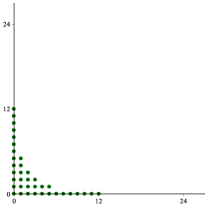
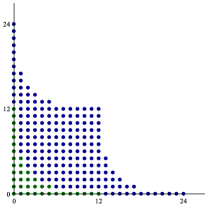
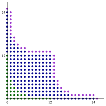
Figure 3.1: $\mathcal{C}_{13}^{2}$, $\mathcal{C}_{13}^{2}+\mathcal{C}_{13}^{2}$ and $\mathcal{C}_{13}^{2}+\mathcal{C}_{13}^{2}+\mathcal{C}_{2}^{2}$.

The evaluation points to be used for sparsity in the generalized Chebyshev basis are $\left({\Theta}_{\omega_{1}}(\xi^{{\alpha}^{{\mathsf{T}}}S}),\ldots,{\Theta}_{\omega_{n}}(\xi^{{\alpha}^{{\mathsf{T}}}S})\right)$ for $\xi=\xi_{0}^{D},\xi_{0}\in\mathbb{N}$, $\xi_{0}>\frac{9}{4}|\mathcal{W}|^{2}$ as described in Theorem 2.27. This can be recognized to generalize sparse interpolation in terms of univariate Chebyshev polynomials [5, 22, 35, 49].

In Section 4 we then show how to recover the support of a linear form. More precisely, we provide the algorithms to solve the following two problems. Given $r\in\mathbb{N}$:

1. Consider the unknowns $\zeta_{1},\ldots,\zeta_{r}\in\mathbb{K}^{n}$ and $a_{1},\ldots,a_{r}\in\mathbb{K}$. They define the linear form

   $$\Omega:\begin{array}[t]{ccl}\mathbb{K}[x^{\pm}]&\rightarrow&\mathbb{K}\\ p&\mapsto&\sum_{i=1}^{r}a_{i}\,p(\zeta_{i})\end{array}$$

   that we write as $\Omega=\sum_{i=1}^{r}a_{i}\,\mathbbm{e}_{\zeta_{i}},$ where $\mathbbm{e}_{\zeta_{i}}(p)=p(\zeta_{i})$. From the values of $\Omega$ on $\left\{x^{\alpha+\beta+\gamma}\,|\,\alpha\in\mathcal{C}_{r}^{n},|\gamma|\leq 1\right\}$, Algorithm 4.8 retrieves the set of pairs $\left\{(a_{1},\zeta_{1}),\ldots,(a_{r},\zeta_{r})\right\}$.

2. Consider the Weyl group $\mathcal{W}$ acting on $({\mathbb{K}}^{*})^{n}$ as in 2.2 , the unknowns $\zeta_{1},\ldots,\zeta_{r}\in\mathbb{K}^{n}$ and $a_{1},\ldots,a_{r}\in\mathbb{K}^{*}$. They define the $\chi$-invariant linear form

   $$\Omega:\begin{array}[t]{ccl}\mathbb{K}[x^{\pm}]&\rightarrow&\mathbb{K}\\ p&\mapsto&\displaystyle\sum_{i=1}^{r}a_{i}\sum_{A\in\mathcal{W}}\chi(A)\,p(A\star\zeta_{i})\end{array}$$

   that we write as $\Omega=\sum_{i=1}^{r}a_{i}\sum_{A\in\mathcal{W}}\chi(A)\,\mathbbm{e}_{A\star\zeta_{i}}.$ From the values of $\Omega$ on $\left\{{\Theta}_{\alpha}{\Theta}_{\beta}{\Theta}_{\gamma}\ \,|\,\alpha,\beta\in\mathcal{C}_{r}^{n},|\gamma|\leq 1\right\}$ if $\chi(A)=1$, or $\left\{{\Upsilon}_{\delta+\alpha}{\Theta}_{\beta}{\Theta}_{\gamma}\ \,|\,\alpha,\beta\in\mathcal{C}_{r}^{n},|\gamma|\leq 1\right\}$ if $\chi(A)=\det(A)$, Algorithm 4.15 retrieves the set of pairs $\left\{(\tilde{a}_{1},\vartheta_{1}),\ldots,(\tilde{a}_{r},\vartheta_{r})\right\}$, where

   • $\tilde{a}_{i}=a_{i}\,{\Theta}_{0}(\zeta_{i})=a_{i}\,|\mathcal{W}|$ or $\tilde{a}_{i}=a_{i}\,{\Upsilon}_{\delta}(\zeta_{i})\neq 0$ depending whether $\chi=1$ or $\det$;

   • $\vartheta_{i}=\left[{\Theta}_{\omega_{1}}(\xi^{{\beta}_{i}^{{\mathsf{T}}}S}),\;\ldots,\;{\Theta}_{\omega_{n}}(\xi^{{\beta}_{i}^{{\mathsf{T}}}S})\right]$.

The second problem appears as a special case of the first one, yet the special treatment allows one to reduce the size of the matrices by a factor $|\mathcal{W}|$. These algorithms rely solely on linear algebra operations and evaluations of polynomial functions:

• Determine a nonsingular principal submatrix of size $r$ in a matrix of size $|\mathcal{C}_{r}^{n}|$ ;

• Compute the generalized eigenvectors of a pair of matrices of size $r\times r$;

• Solve a nonsingular square linear system of size $r$.

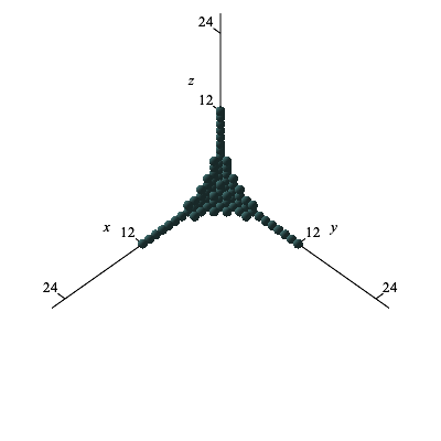
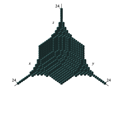
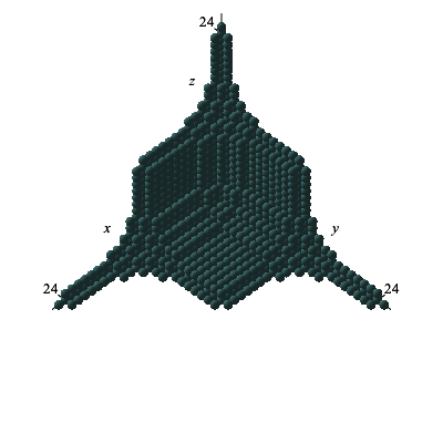
Figure 3.2: $\mathcal{C}_{13}^{3}$, $\mathcal{C}_{13}^{3}+\mathcal{C}_{13}^{3}$ and $\mathcal{C}_{13}^{3}+\mathcal{C}_{13}^{3}+\mathcal{C}_{2}^{3}$.

3.1 Sparse interpolation of a Laurent polynomial in the monomial basis

Consider a Laurent polynomial in $n$ variables that is $r$-sparse in the monomial basis. This means that

$$f=\sum_{i=1}^{r}a_{i}\,x^{\beta_{i}},$$

for some $a_{i}\in{\mathbb{K}}^{*}$ and $\beta_{i}\in\mathbb{Z}^{n}$. The function it defines is a black box: we can evaluate it at chosen points but know neither its coefficients $\left\{a_{1},\ldots,a_{r}\right\}\subset{\mathbb{K}}^{*}$ nor its support $\left\{\beta_{1},\ldots,\beta_{r}\right\}\subset\mathbb{Z}^{n}$; only the size $r$ of its support. The problem we address is to find the pairs $(a_{i},\beta_{i})\in{\mathbb{K}}^{*}\times\mathbb{Z}^{n}$ from a small set of evaluations of $f$

To $\displaystyle f=\sum_{i=1}^{r}a_{i}\,x^{\beta_{i}}$ and $\xi\in\mathbb{Q},\;\xi>1$, we associate the linear form

$$\Omega:\begin{array}[t]{ccl}\mathbb{K}[x^{\pm}]&\rightarrow&\mathbb{K}\\ p&\mapsto&\displaystyle\sum_{i=1}^{r}a_{i}\,p(\zeta_{i})\quad\hbox{ where }\quad\zeta_{i}=\xi^{{\beta}_{i}^{{\mathsf{T}}}}=\begin{bmatrix}\xi^{\beta_{i,1}}&\ldots&\xi^{\beta_{i,n}}\end{bmatrix}\in({\mathbb{K}}^{*})^{n}.\end{array}$$

By denoting $\mathbbm{e}_{\zeta}$ the linear form that is the evaluation at $\zeta\in\mathbb{K}^{n}$ we can write $\Omega=\sum_{i=1}^{r}a_{i}\mathbbm{e}_{\zeta_{i}}.$ We observe that

$$\Omega\left(x^{\alpha}\right)=\sum_{i=1}^{r}a_{i}\left(\xi^{{\beta}_{i}^{{\mathsf{T}}}}\right)^{\alpha}=\sum_{i=1}^{r}a_{i}\left(\xi^{{\alpha}^{{\mathsf{T}}}}\right)^{\beta_{i}}=f\left(\xi^{{\alpha}^{{\mathsf{T}}}}\right)$$

since ${\beta}^{{\mathsf{T}}}\alpha={\alpha}^{{\mathsf{T}}}\beta$. In other words, the value of $\Omega$ on the monomial basis $\left\{x^{\alpha}\,|\,\alpha\in\mathbb{N}^{n}\right\}$ is known from the evaluation of $f$ at the set of points $\left\{\xi^{{\alpha}^{{\mathsf{T}}}}\,|\,\alpha\in\mathbb{N}^{n}\right\}\subset({\mathbb{K}}^{*})^{n}$. Though trite in the present case, a commutation property such as ${\beta}^{{\mathsf{T}}}\alpha={\alpha}^{{\mathsf{T}}}\beta$ is at the heart of sparse interpolation algorithms.

Algorithm 3.1

LaurentInterpolation

Input: $r\in\mathbb{N}_{>0}$, $\xi\in\mathbb{Q}$, $\xi>1$, and a function $f$ that can be evaluated at arbitrary points and is known to be a sum of $r$ monomials.

Output: The pairs $(a_{1},\beta_{1}),\ldots,(a_{r},\beta_{r})\in{\mathbb{K}}^{*}\times\mathbb{Z}^{n}$ such that $\displaystyle f=\sum_{i=1}^{r}a_{i}\,x^{\beta_{i}}$

• Perform the evaluations of $f$ on $\left\{\left(\xi^{{(\gamma+\alpha+\beta)}^{{\mathsf{T}}}}\right)\;|\;\alpha,\beta\in\mathcal{C}_{r}^{n},\,|\gamma|\leq 1\right\}\subset\mathbb{Q}^{n}$.

• Apply Algorithm 4.8(Support & Coefficients) to determine the pairs $(a_{1},\zeta_{1}),\ldots,(a_{r},\zeta_{r})\in{\mathbb{K}}^{*}\times({\mathbb{K}}^{*})^{n}$ such that the linear form $\Omega=\sum_{i=1}^{r}a_{i}\,\mathbbm{e}_{\zeta_{i}}$ satisfies $\Omega(x^{\alpha})=f(\xi^{\alpha}).$

• For $1\leq i\leq r$, determine $\beta_{i}$ from $\zeta_{i}$ by taking logarithms. Indeed $\zeta_{i}=\xi^{{\beta}_{i}^{{\mathsf{T}}}}$. Hence for $1\leq i\leq r$ and $1\leq j\leq n$

  $$\zeta_{i,j}=\xi^{\beta_{i,j}}\hbox{ so that }\beta_{i,j}=\frac{\ln(\zeta_{i,j})}{\ln(\xi)}$$

Example 3.2

In $\mathbb{K}[x,y,x^{-1},y^{-1}]$, let us consider a 2-sparse polynomial in the monomial basis. Thus $f(x,y)=a\,x^{\alpha_{1}}y^{\alpha_{2}}+b\,x^{\beta_{1}}y^{\beta_{2}}$. We have

$$\mathcal{C}_{2}^{2}=\left\{{\begin{bmatrix}0&0\end{bmatrix}}^{{\mathsf{T}}},{\begin{bmatrix}1&0\end{bmatrix}}^{{\mathsf{T}}},{\begin{bmatrix}0&1\end{bmatrix}}^{{\mathsf{T}}}\right\}.$$

Hence

$$\left\{\alpha+\beta+\gamma\,|\,\alpha,\beta\in\mathcal{C}_{2}^{2},|\gamma|\leq 1\right\}=\left\{[0,0],[0,1],[0,2],[0,3],[1,0],[1,1],[1,2],[2,0],[2,1],[3,0]\right\}.$$

To retrieve the pairs $(a,\alpha)$ and $(b,\beta)$ in ${\mathbb{K}}^{*}\times\mathbb{N}^{2}$ one thus need to evaluate $f$ at the points

$$\left\{[1,1],[1,\xi],[1,{\xi}^{2}],[1,{\xi}^{3}],[\xi,1],[\xi,\xi],[\xi,{\xi}^{2}],[{\xi}^{2},1],[{\xi}^{2},\xi],[{\xi}^{3},1]\right\}\subset\mathbb{Q}^{2}$$

From these values, Algorithm 4.8 will recover the pairs

$$\left(a,[\xi^{\alpha_{1}},\xi^{\alpha_{2}}]\right),\left(b,[\xi^{\beta_{1}},\xi^{\beta_{2}}]\right).$$

Taking some logarithms on this output we get $(a,\alpha),(b,\beta).$

3.2 Sparse interpolation with Chebyshev polynomials of the first kind

We consider now the polynomial ring $\mathbb{K}[X]=\mathbb{K}[X_{1},\ldots,X_{n}]$ and a black box function $F$ that is a $r$-sparse polynomial in the basis of Chebyshev polynomials $\left\{T_{\beta}\right\}_{\beta\in\mathbb{N}^{n}}$ of the first kind associated to the Weyl group $\mathcal{W}$:

$$F(X_{1},\ldots,X_{n})=\sum_{i=1}^{r}a_{i}\,T_{\beta_{i}}(X_{1},\ldots,X_{n})\in\mathbb{K}[X_{1},\ldots,X_{n}].$$

By Definition 2.12, $T_{\beta}\left({\Theta}_{\omega_{1}}(x),\ldots,{\Theta}_{\omega_{n}}(x)\right)={\Theta}_{\beta}(x)$ where ${\Theta}_{\beta}(x)=\sum_{A\in\mathcal{W}}x^{A\beta}$. Upon introducing

$$f(x)=F({\Theta}_{\omega_{1}}(x),\ldots,{\Theta}_{\omega_{n}}(x))=\sum_{i=1}^{r}a_{i}\sum_{A\in\mathcal{W}}x^{A\beta_{i}}$$

we could apply Algorithm 3.1 to recover the pairs $(a_{i},A\beta_{i})$. Instead we examine how to recover the pairs $(a_{i},\beta_{i})$ only. For that we associate to $F$ and $\xi\in\mathbb{N}$, $\xi>0$, the linear form

$$\Omega:\begin{array}[t]{ccl}\mathbb{K}[x^{\pm}]&\rightarrow&\mathbb{K}\\ p&\mapsto&\displaystyle\sum_{i=1}^{r}a_{i}\sum_{A\in\mathcal{W}}p(A\star\zeta_{i})\quad\hbox{ where }\quad\zeta_{i}=\xi^{{\beta}_{i}^{{\mathsf{T}}}S}\in({\mathbb{K}}^{*})^{n}.\end{array}$$

The linear form $\Omega$ is $\mathcal{W}$-invariant, that is $\Omega\left(A\cdot p\right)=\Omega\left(p\right)$. The property relevant to sparse interpolation is that the value of $\Omega$ on $\left\{{\Theta}_{\alpha}\right\}_{\alpha\in\mathbb{N}^{n}}$ is obtained by evaluating $F$.

Proposition 3.3

$\displaystyle\Omega({\Theta}_{\alpha})=F\left({\Theta}_{\omega_{1}}(\xi^{{\alpha}^{{\mathsf{T}}}S}),\ldots,{\Theta}_{\omega_{n}}(\xi^{{\alpha}^{{\mathsf{T}}}S})\right)$.

The proof of this proposition is a consequence of the following commutation property.

Lemma 3.4

Consider $\chi:\mathcal{W}\rightarrow\mathbb{K}^{*}$ a group morphism such that $\chi(A)^{2}=1$ for all $A\in\mathcal{W}$, and ${\Psi}^{\chi}_{\alpha}=\sum_{A\in\mathcal{W}}\chi(A)^{-1}\,x^{A\alpha}.$ If $S$ is a positive definite symmetric matrix such that ${A}^{{\mathsf{T}}}SA=S$ for all $A\in\mathcal{W}$, then for any $\xi\in{\mathbb{K}}^{*}$

$${\Psi}^{\chi}_{\alpha}\left(\xi^{{\beta}^{{\mathsf{T}}}S}\right)={\Psi}^{\chi}_{\beta}\left(\xi^{{\alpha}^{{\mathsf{T}}}S}\right),$$

where $\displaystyle{\Psi}^{\chi}_{\alpha}=\sum_{B\in\mathcal{W}}\chi(B)^{-1}\,x^{B\alpha}$ as defined in (2.3).

Proof.

We have

$${\Psi}^{\chi}_{\alpha}\left(\xi^{{\beta}^{{\mathsf{T}}}S}\right)=\sum_{A\in\mathcal{W}}\chi(A)^{-1}\,\left(\xi^{{\beta}^{{\mathsf{T}}}S}\right)^{A\alpha}=\sum_{A\in\mathcal{W}}\chi(A)^{-1}\,\xi^{{\beta}^{{\mathsf{T}}}S{A\alpha}}.$$

Since ${A}^{{\mathsf{T}}}SA=S$, we have $SA={A}^{{-\mathsf{T}}}S$ so that

$${\Psi}^{\chi}_{\alpha}\left(\xi^{{\beta}^{{\mathsf{T}}}S}\right)=\sum_{A\in\mathcal{W}}\chi(A)^{-1}\,\xi^{{\beta}^{{\mathsf{T}}}{A}^{{-\mathsf{T}}}S\alpha}=\sum_{A\in\mathcal{W}}\chi(A)^{-1}\,\xi^{{(A^{-1}\beta)}^{{\mathsf{T}}}S\alpha}.$$

Since, trivially, ${\beta}^{{\mathsf{T}}}S\alpha={\alpha}^{{\mathsf{T}}}S\beta$ for all $\alpha,\beta\in\mathbb{Z}^{n}$, we have

$${\Psi}^{\chi}_{\alpha}\left(\xi^{{\beta}^{{\mathsf{T}}}S}\right)=\sum_{A\in\mathcal{W}}\chi(A)^{-1}\,\xi^{{\alpha}^{{\mathsf{T}}}S{(A^{-1}\beta)}}=\sum_{A\in\mathcal{W}}\chi(A)^{-1}\left(\xi^{{\alpha}^{{\mathsf{T}}}S}\right)^{A^{-1}\beta}.$$

The conclusion comes from the fact that $\chi(A)^{2}=1$ implies that $\chi(A)=\chi(A)^{-1}$.    $\Box$

proof of proposition 3.3: When $\chi(A)=1$ for all $A\in\mathcal{W}$ we have ${\Psi}^{1}_{\alpha}={\Theta}_{\alpha}$. Therefore Lemma 3.4 implies

$$F\left({\Theta}_{\omega_{1}}(\xi^{{\alpha}^{{\mathsf{T}}}S}),\ldots,{\Theta}_{\omega_{n}}(\xi^{{\alpha}^{{\mathsf{T}}}S})\right) = \sum_{i=1}^{r}a_{i}\,T_{\beta_{i}}\left({\Theta}_{\omega_{1}}(\xi^{{\alpha}^{{\mathsf{T}}}S}),\ldots,{\Theta}_{\omega_{n}}(\xi^{{\alpha}^{{\mathsf{T}}}S})\right)$$

$$= \sum_{i=1}^{r}a_{i}\,{\Theta}_{\beta_{i}}\left(\xi^{{\alpha}^{{\mathsf{T}}}S}\right)\;=\;\sum_{i=1}^{r}a_{i}\,{\Theta}_{\alpha}\left(\xi^{{\beta}_{i}^{{\mathsf{T}}}S}\right)\;=\;\Omega({\Theta}_{\alpha}).$$

$\blacksquare$

In the following algorithm to recover the support of $F$ we need to have the value of $\Omega$ on the polynomials ${\Theta}_{\alpha}{\Theta}_{\beta}{\Theta}_{\gamma}$ for $\alpha,\beta\in\mathcal{C}_{r}^{n}$ and $|\gamma|\leq 1$. We have access to the values of $\Omega$ on ${\Theta}_{\mu}$, for any $\mu\in\mathbb{N}^{n}$, by evaluating $F$ at $\left({\Theta}_{\omega_{1}}(\xi^{{\mu}^{{\mathsf{T}}}S}),\ldots,{\Theta}_{\omega_{n}}(\xi^{{\mu}^{{\mathsf{T}}}S})\right)$. To get the values of $\Omega$ on ${\Theta}_{\alpha}{\Theta}_{\beta}{\Theta}_{\gamma}$ we consider the relationships stemming from Proposition 2.22

$${\Theta}_{\gamma}{\Theta}_{\alpha}{\Theta}_{\beta}=\sum_{\nu\in S(\alpha,\beta,\gamma)}a_{\nu}\,{\Theta}_{\nu}$$

where $S(\alpha,\beta,\gamma)$ is a finite subset of $\left\{\mu\in\mathbb{N}^{n}\,|\,\mu\prec\alpha+\beta+\gamma\right\}$. Then the set

$$\mathfrak{X}_{r}^{\mathcal{W}}=\bigcup_{\begin{subarray}{c}\alpha,\beta\in\mathcal{C}_{r}^{n}\\ |\gamma|\leq 1\end{subarray}}S(\alpha,\beta,\gamma)$$ (3.1)

indexes the evaluations needed to determine the support of a $r$-sparse sum of Chebyshev polynomials associated to the Weyl group $\mathcal{W}$.

As we noted in the paragraph preceding Lemma 2.25, the entries of $S$ are in $\mathbb{Q}$ and we shall denote by $D$ the least common denominator of these entries.

Algorithm 3.5

FirstKindInterpolation

Input: $r\in\mathbb{N}_{>0}$, $\xi_{0}\in\mathbb{N}_{>0}$, where $\xi_{0}>\left(\frac{3}{2}|\mathcal{W}|\right)^{2}$ and $\xi=\xi_{0}^{D}$, and a function $F$ that can be evaluated at arbitrary points and is known to be the sum of $r$ generalized Chebyshev polynomials of the first kind.

Output: The pairs $(a_{1},\beta_{1}),\ldots,(a_{r},\beta_{r})\in{\mathbb{K}}^{*}\times\mathbb{Z}^{n}$ such that

$$F(X_{1},\ldots,X_{n})=\sum_{i=1}^{r}a_{i}\,T_{\beta_{i}}(X_{1},\ldots,X_{n}).$$

• From the evaluations $\left\{\left.F\left({\Theta}_{\omega_{1}}(\xi^{{\alpha}^{{\mathsf{T}}}S}),\ldots,{\Theta}_{\omega_{n}}(\xi^{{\alpha}^{{\mathsf{T}}}S})\right)\;\right|\;\alpha\in\mathfrak{X}_{r}^{\mathcal{W}}\right\}$ determine $\left\{\left.\Omega({\Theta}_{\alpha}{\Theta}_{\beta}{\Theta}_{\gamma})\;\right|\;\alpha,\beta\in\mathcal{C}_{r}^{n},\,|\gamma|\leq 1\right\}$

  % The hypothesis on $\xi=\xi_{0}^{D}$ guarantees that $\xi^{{\alpha}^{{\mathsf{T}}}S}$ is a row vector of integers.

• Apply Algorithm 4.15 (Invariant Support & Coefficients) to calculate the vectors

  $$\vartheta_{i}=\left[{\Theta}_{\omega_{1}}(\xi^{{\beta}_{i}^{{\mathsf{T}}}S}),\;\ldots,\;{\Theta}_{\omega_{n}}(\xi^{{\beta}_{i}^{{\mathsf{T}}}S})\right],\quad 1\leq i\leq r$$

  and the vector $\left[\tilde{a}_{1},\ldots,\tilde{a}_{r}\right]=\left[|\mathcal{W}|\,{a}_{1},\ldots,|\mathcal{W}|\,{a}_{r}\right].$

• Deduce $\left[{a}_{1},\ldots,{a}_{r}\right].$

• Calculate

  $$\left[{\Theta}_{\beta_{i}}\left(\xi^{{\mu}_{1}^{{\mathsf{T}}}S}\right),\;\ldots,\;{\Theta}_{\beta_{i}}\left(\xi^{{\mu}_{n}^{{\mathsf{T}}}S}\right)\right]=\left[T_{\mu_{1}}(\vartheta_{i}),\;\ldots,\;T_{\mu_{n}}(\vartheta_{i})\right]$$

  using the precomputed Chebyshev polynomials $\{T_{\mu_{1}},\ldots,T_{\mu_{n}}\}$, where $\mu_{1},\ldots,\mu_{n}$ are linearly independent strongly dominant weights.

• Using Theorem 2.27, recover each $\beta_{i}$ from

  $$\left[{\Theta}_{\beta_{i}}\left(\xi^{{\mu}_{1}^{{\mathsf{T}}}S}\right),\;\ldots,\;{\Theta}_{\beta_{i}}\left(\xi^{{\mu}_{n}^{{\mathsf{T}}}S}\right)\right].$$

As will be remarked after its description, Algorithm 4.15 may, in some favorable cases, return directly the vector

$$\left[{\Theta}_{\mu_{j}}(\xi^{{\beta}_{1}^{{\mathsf{T}}}S}),\ldots,{\Theta}_{\mu_{j}}(\xi^{{\beta}_{r}^{{\mathsf{T}}}S})\right]=\left[{\Theta}_{\beta_{1}}(\xi^{{\mu}_{j}^{{\mathsf{T}}}S}),\ldots,{\Theta}_{\beta_{r}}(\xi^{{\mu}_{j}^{{\mathsf{T}}}S})\right].$$

for some or all $1\leq j\leq n$. This then saves on evaluating $T_{\mu_{j}}$ at the points $\vartheta_{1},\,\ldots,\,\vartheta_{r}$.

Example 3.6

We consider the Chebyshev polynomials of the first kind $\left\{T_{\alpha}\right\}_{\alpha\in\mathbb{N}^{2}}$ associated to the Weyl group $\mathcal{A}_{2}$ and a 2-sparse polynomial $F(X,Y)=a\,T_{\alpha}(X,Y)+b\,T_{\beta}(X,Y)$ in this basis of $\mathbb{K}[X,Y]$.

We need to consider

$$\mathcal{C}_{2}^{2}=\left\{{\begin{bmatrix}0&0\end{bmatrix}}^{{\mathsf{T}}},{\begin{bmatrix}1&0\end{bmatrix}}^{{\mathsf{T}}},{\begin{bmatrix}0&1\end{bmatrix}}^{{\mathsf{T}}}\right\}.$$

The following relations

$$\begin{array}[]{l}{{\Theta}_{{0,0}}}^{2}=6\,{\Theta}_{{0,0}},\quad{\Theta}_{{0,0}}{\Theta}_{{0,1}}=6\,{\Theta}_{{0,1}},\quad{\Theta}_{{0,0}}{\Theta}_{{1,0}}=6\,{\Theta}_{{1,0}},\\ {{\Theta}_{{0,1}}}^{2}=2\,{\Theta}_{{0,2}}+4\,{\Theta}_{{1,0}},\quad{\Theta}_{{0,1}}{\Theta}_{{1,0}}=4\,{\Theta}_{{1,1}}+2\,{\Theta}_{{0,0}},\quad{{\Theta}_{{1,0}}}^{2}=2\,{\Theta}_{{2,0}}+4\,{\Theta}_{{0,1}}\end{array}$$

and

$$\begin{array}[]{l}{\Theta}_{{2,0}}{\Theta}_{{0,0}}=6\,{\Theta}_{{2,0}},\quad{\Theta}_{{2,0}}{\Theta}_{{1,0}}=2\,{\Theta}_{{3,0}}+4\,{\Theta}_{{1,1}},\quad{\Theta}_{{2,0}}{\Theta}_{{0,1}}=4\,{\Theta}_{{2,1}}+2\,{\Theta}_{{1,0}},\\ {\Theta}_{{1,1}}{\Theta}_{{0,0}}=6\,{\Theta}_{{1,1}},\quad{\Theta}_{{1,1}}{\Theta}_{{1,0}}=2\,{\Theta}_{2,1}+2\,{\Theta}_{0,2}+2\,{\Theta}_{1,0},\quad{\Theta}_{{1,1}}{\Theta}_{{0,1}}=2\,{\Theta}_{1,2}+2\,{\Theta}_{2,0}+2\,{\Theta}_{0,1},\\ {\Theta}_{{0,2}}{\Theta}_{{0,0}}=6\,{\Theta}_{{0,2}},\quad{\Theta}_{{0,2}}{\Theta}_{{1,0}}=4\,{\Theta}_{{1,2}}+2\,{\Theta}_{{0,1}},\quad{\Theta}_{{0,2}}{\Theta}_{{0,1}}=2\,{\Theta}_{{0,3}}+4\,{\Theta}_{{1,1}},\end{array}$$

allow one to express any product ${\Theta}_{\alpha}{\Theta}_{\beta}{\Theta}_{\gamma}$, $\alpha,\beta\in\mathcal{C}_{2}^{n}$, $|\gamma|\leq 1$ as a linear combination of elements from $\{{\Theta}_{\alpha}\ |\ \alpha\in\mathfrak{X}_{2}^{\mathcal{A}_{2}}\}$ where

$$\mathfrak{X}_{2}^{\mathcal{A}_{2}}=\left\{[0,0],[0,1],[0,2],[0,3],[1,0],[1,1],[1,2],[2,0],[2,1],[3,0]\right\}.$$

For example ${\Theta}_{1,0}{\Theta}_{0,1}^{2}=8{\Theta}_{1,2}+20{\Theta}_{0,1}+8{\Theta}_{2,0}$.

We consider

$$f(x,y) = F\left({\Theta}_{\omega_{1}}(x,y),{\Theta}_{\omega_{2}}(x,y)\right)$$

where

$${\Theta}_{\omega_{1}}(x,y)=2\,x+2\,{y}{x}^{-1}+2\,{y}^{-1},\hbox{ and }{\Theta}_{\omega_{2}}(x,y)=2\,y+2\,{x}{y}^{-1}+2\,{x}^{-1}.$$

We introduce the invariant linear form $\Omega$ on $\mathbb{K}[x,y,x^{-1},y^{-1}]$ determined by $\Omega({\Theta}_{\gamma})=f\left(\xi^{\frac{2}{3}\gamma_{1}+\frac{1}{3}\gamma_{2}},\xi^{\frac{1}{3}\gamma_{1}+\frac{2}{3}\gamma_{2}}\right)$ The first step of the algorithm requires us to determine $\left\{\left.\Omega({\Theta}_{\alpha}{\Theta}_{\beta}{\Theta}_{\gamma})\;\right|\;\alpha,\beta\in\mathcal{C}_{2}^{2},\,|\gamma|\leq 1\right\}$. Expanding these triple products as linear combinations of orbit polynomials, we see from Proposition 3.3 that to determine these values it is enough to evaluate $f(x,y)$ at the 10 points $\{\xi^{{\alpha}^{{\mathsf{T}}}S}\ |\ \alpha\in\mathfrak{X}_{2}^{\mathcal{A}_{2}}\}$, that is, at the points

$$\left\{[1,1],[\xi^{\frac{1}{3}},\xi^{\frac{2}{3}}],[\xi^{\frac{2}{3}},\xi^{\frac{4}{3}}],[\xi,\xi^{2}],[\xi^{\frac{2}{3}},\xi^{\frac{1}{3}}],[\xi,\xi],[\xi^{\frac{4}{3}},\xi^{\frac{5}{3}}],[\xi^{\frac{4}{3}},\xi^{\frac{2}{3}}],[\xi^{\frac{5}{3}},\xi^{\frac{4}{3}}],[\xi^{2},\xi]\right\}$$

Note that $D=3$ so $\xi=({\xi}_{0})^{3}$ for some $\xi_{0}\in\mathbb{N}_{>0}$. Therefore the above vectors have integer entries.

From these values, Algorithm 4.15 will recover the pairs $(a,\vartheta_{\alpha})$ and $(b,\vartheta_{\beta})$ where

$$\vartheta_{\alpha}=[{\Theta}_{\omega_{1}}(\xi^{{\alpha}^{{\mathsf{T}}}S}),{\Theta}_{\omega_{2}}(\xi^{{\alpha}^{{\mathsf{T}}}S})]\;\mbox{ and }\;\vartheta_{\beta}=[{\Theta}_{\omega_{1}}(\xi^{{\beta}^{{\mathsf{T}}}S}),{\Theta}_{\omega_{2}}(\xi^{{\beta}^{{\mathsf{T}}}S})].$$

One can then form

$$[T_{\mu_{1}}(\vartheta_{\alpha}),T_{\mu_{2}}(\vartheta_{\alpha})]=\left[{\Theta}_{\alpha}(\xi^{{\mu}_{1}^{{\mathsf{T}}}S}),{\Theta}_{\alpha}(\xi^{{\mu}_{2}^{{\mathsf{T}}}S})\right]$$

and

$$[T_{\mu_{1}}(\vartheta_{\beta}),T_{\mu_{2}}(\vartheta_{\beta})]=\left[{\Theta}_{\beta}(\xi^{{\mu}_{1}^{{\mathsf{T}}}S}),{\Theta}_{\beta}(\xi^{{\mu}_{2}^{{\mathsf{T}}}S})\right]$$

using the polynomials calculated in Example 2.13 and find $\alpha$ and $\beta$ as illustrated in Example 2.28.

Note that the function $f$ is a 12-sparse polynomial in the monomial basis

$$f(x,y) = a\,{\Theta}_{\alpha}(x)+b\,{\Theta}_{\beta}(x)$$

$$= a\left({x}^{\alpha_{{1}}}{y}^{\alpha_{{2}}}+{x}^{-\alpha_{{1}}}{y}^{\alpha_{{1}}+\alpha_{{2}}}+{x}^{\alpha_{{1}}+\alpha_{{2}}}{y}^{-\alpha_{{2}}}+{x}^{\alpha_{{2}}}{y}^{-\alpha_{{1}}-\alpha_{{2}}}+{x}^{-\alpha_{{1}}-\alpha_{{2}}}{y}^{\alpha_{{1}}}+{x}^{-\alpha_{{2}}}{y}^{-\alpha_{{1}}}\right)$$

$$+b\left({x}^{\beta_{{1}}}{y}^{\beta_{{2}}}+{x}^{-\beta_{{1}}}{y}^{\beta_{{1}}+\beta_{{2}}}+{x}^{\beta_{{1}}+\beta_{{2}}}{y}^{-\beta_{{2}}}+{x}^{\beta_{{2}}}{y}^{-\beta_{{1}}-\beta_{{2}}}+{x}^{-\beta_{{1}}-\beta_{{2}}}{y}^{\beta_{{1}}}+{x}^{-\beta_{{2}}}{y}^{-\beta_{{1}}}\right),$$

Yet to retrieve its support we only need to evaluate $f$ at points indexed by $\mathfrak{X}_{2}^{\mathcal{A}_{2}}$, which is equal to $\mathcal{C}_{2}^{2}+\mathcal{C}_{2}^{2}+\mathcal{C}_{2}^{2}$ and has cardinality $10$.

Note though that $12$ is actually an upper bound on the sparsity of $f$ in the monomial basis. If $\alpha$ or $\beta$ has a component that is zero then the actual sparsity can be $4$, $6$, $7$ or $9$. We shall comment on dealing with upper bounds on the sparsity rather than the exact sparsity in Section 5.

3.3 Sparse interpolation with Chebyshev polynomials of the second kind

We consider now the polynomial ring $\mathbb{K}[X]=\mathbb{K}[X_{1},\ldots,X_{n}]$ and a black box function $F$ that is an $r$-sparse polynomial in the basis of Chebyshev polynomials $\left\{U_{\beta}\right\}_{\beta\in\mathbb{N}^{n}}$ of the second kind associated to the Weyl group $\mathcal{W}$. Hence

$$F(X_{1},\ldots,X_{n})=\sum_{i=1}^{r}a_{i}\,U_{\beta_{i}}(X_{1},\ldots,X_{n})\in\mathbb{K}[X_{1},\ldots,X_{n}].$$

By Definition 2.16 and thanks to Theorem 2.17 $U_{\beta}\left({\Theta}_{\omega_{1}}(x),\ldots,{\Theta}_{\omega_{n}}(x)\right)={\Xi}_{\beta}(x)=\frac{{\Upsilon}_{\delta+\beta}(x)}{{\Upsilon}_{\delta}(x)}$. Hence upon introducing

$$f(x)={\Upsilon}_{\delta}(x)\,F({\Theta}_{\omega_{1}}(x),\ldots,{\Theta}_{\omega_{n}}(x))=\sum_{i=1}^{r}a_{i}\,{\Upsilon}_{\delta+\beta_{i}}(x)=\sum_{i=1}^{r}a_{i}\,\sum_{A\in\mathcal{W}}\det(A)^{-1}\,x^{A(\delta+\beta_{i})}$$

we could apply Algorithm 3.1 to recover the pairs $\left(a_{i},A(\delta+\beta_{i})\right)$. We examine how to recover only the pairs $(a_{i},\delta+\beta_{i})$. For that we define

$$\Omega:\begin{array}[t]{ccl}\mathbb{K}[x^{\pm}]&\rightarrow&\mathbb{K}\\ p&\mapsto&\displaystyle\sum_{i=1}^{r}a_{i}\sum_{A\in\mathcal{W}}\det(A)\,p(\zeta_{i}^{A})\quad\hbox{ where }\quad\zeta_{i}=\xi^{{(\delta+\beta_{i})}^{{\mathsf{T}}}S}\in({\mathbb{K}}^{*})^{n}.\end{array}$$

The linear form $\Omega$ is skew invariant, i.e. $\Omega\left(A\cdot p\right)=\det(A)^{-1}\,\Omega\left(p\right)$. The property relevant to sparse interpolation is that the value of $\Omega$ on $\left\{{\Upsilon}_{\alpha}\right\}_{\alpha\in\mathbb{N}^{n}}$ is obtained by evaluating $F$.

Proposition 3.7

$\displaystyle\Omega({\Upsilon}_{\alpha})={\Upsilon}_{\delta}\left(\xi^{{\alpha}^{{\mathsf{T}}}S}\right)\,F\left({\Theta}_{\omega_{1}}(\xi^{{\alpha}^{{\mathsf{T}}}S}),\ldots,{\Theta}_{\omega_{n}}(\xi^{{\alpha}^{{\mathsf{T}}}S})\right)$

Proof.

Note that $\displaystyle F({\Theta}_{\omega_{1}}(x),\ldots,{\Theta}_{\omega_{n}}(x))=\sum_{i=1}^{r}{a}_{i}\,{\Xi}_{\beta_{i}}(x)$ so that $\displaystyle{\Upsilon}_{\delta}(x)\,F({\Theta}_{\omega_{1}}(x),\ldots,{\Theta}_{\omega_{n}}(x))=\sum_{i=1}^{r}{a}_{i}\,{\Upsilon}_{\delta+\beta_{i}}(x)$.

Lemma 3.4 implies

$${\Upsilon}_{\delta}(\xi^{{\alpha}^{{\mathsf{T}}}S})\,F\left({\Theta}_{\omega_{1}}(\xi^{{\alpha}^{{\mathsf{T}}}S}),\ldots,{\Theta}_{\omega_{n}}(\xi^{{\alpha}^{{\mathsf{T}}}S})\right) = \sum_{i=1}^{r}a_{i}\,{\Upsilon}_{\delta+\beta_{i}}\left(\xi^{{\alpha}^{{\mathsf{T}}}S}\right)$$

$$= \sum_{i=1}^{r}a_{i}\,{\Upsilon}_{\alpha}\left(\xi^{{(\delta+\beta_{i})}^{{\mathsf{T}}}S}\right)\;=\;\Omega({\Upsilon}_{\alpha}).$$

$\Box$

We are now in a position to describe the algorithm to recover the support of $F$ from its evaluations at a set of points $\left\{\left({\Theta}_{\omega_{1}}(\xi^{{\alpha}^{{\mathsf{T}}}S}),\ldots,{\Theta}_{\omega_{n}}(\xi^{{\alpha}^{{\mathsf{T}}}S})\right)\;|\;{\alpha\in\check{\mathfrak{X}}_{r}^{\mathcal{W}}}\right\}$. The set $\check{\mathfrak{X}}_{r}^{\mathcal{W}}$ is defined similarly to the set $\mathfrak{X}_{r}^{\mathcal{W}}$ in the previous section (Equation 3.1).

$$\check{\mathfrak{X}}_{r}^{\mathcal{W}}=\bigcup_{\begin{subarray}{c}\alpha,\beta\in\mathcal{C}_{r}^{n}\\ |\gamma|\leq 1\end{subarray}}\check{S}(\alpha,\beta,\gamma)$$ (3.2)

where the subsets $\check{S}(\alpha,\beta,\gamma)$ of $\left\{\mu\in\delta+\mathbb{N}^{n}\,|\,\mu\prec\delta+\alpha+\beta+\gamma\right\}$ are defined by the fact that

$${\Upsilon}_{\delta+\alpha}{\Theta}_{\beta}{\Theta}_{\gamma}=\sum_{\nu\in\check{S}(\alpha,\beta,\gamma)}a_{\nu}\,{\Upsilon}_{\nu}.$$

Algorithm 3.8

SecondKindInterpolation

Input: $r\in\mathbb{N}_{>0}$, $\xi_{0}\in\mathbb{N}_{>0}$, where $\xi_{0}>(\frac{3}{2}|\mathcal{W}|)^{2}$ and $\xi=\xi_{0}^{D}$ , and a function $F$ that can be evaluated at arbitrary points and is known to be the sum of $r$ generalized Chebyshev polynomials of the second kind.

Output: The pairs $(a_{1},\beta_{1}),\ldots,(a_{r},\beta_{r})\in{\mathbb{K}}^{*}\times\mathbb{Z}^{n}$ such that

$$F(X_{1},\ldots,X_{n})=\sum_{i=1}^{r}a_{i}\,U_{\beta_{i}}(X_{1},\ldots,X_{n}).$$

• From $\left\{\left.{\Upsilon}_{\delta}(\xi^{{\alpha}^{{\mathsf{T}}}S})F\left({\Theta}_{\omega_{1}}(\xi^{{\alpha}^{{\mathsf{T}}}S}),\ldots,{\Theta}_{\omega_{n}}(\xi^{{\alpha}^{{\mathsf{T}}}S})\right)\;\right|\;\alpha\in\check{\mathfrak{X}}_{r}^{\mathcal{W}}\right\}$ determine $\left\{\left.\Omega({\Upsilon}_{\delta+\alpha}{\Theta}_{\beta}{\Theta}_{\gamma})\;\right|\;\alpha,\beta\in\mathcal{C}_{r}^{n},\,|\gamma|\leq 1\right\}$

• Apply Algorithm 4.15 (Invariant Support & Coefficients) to calculate the vectors

  $$\check{\vartheta}_{i}=\left[{\Theta}_{\omega_{1}}(\xi^{{(\delta+\beta_{i})}^{{\mathsf{T}}}S}),\;\ldots,\;{\Theta}_{\omega_{n}}(\xi^{{(\delta+\beta_{i})}^{{\mathsf{T}}}S})\right],\quad 1\leq i\leq r$$

  and the vector $\left[\tilde{a}_{1},\ldots,\tilde{a}_{r}\right]=\left[{\Upsilon}_{\delta}\left(\xi^{{(\delta+\beta_{1})}^{{\mathsf{T}}}S}\right)\,{a}_{1},\ldots,{\Upsilon}_{\delta}\left(\xi^{{(\delta+\beta_{r})}^{{\mathsf{T}}}S}\right)\,{a}_{r}\right]$

• Calculate

  $$\left[{\Theta}_{\delta+\beta_{i}}\left(\xi^{{\mu}_{1}^{{\mathsf{T}}}S}\right),\;\ldots,\;{\Theta}_{\delta+\beta_{i}}\left(\xi^{{\mu}_{n}^{{\mathsf{T}}}S}\right)\right]=\left[T_{\mu_{1}}(\check{\vartheta}_{i}),\;\ldots,\;T_{\mu_{n}}(\check{\vartheta}_{i})\right]$$

  using the Chebyshev polynomials $\{T_{\mu_{1}},\ldots,T_{\mu_{n}}\}$, where $\mu_{1},\ldots,\mu_{n}$ are linearly independent strongly dominant weights.

• Using Theorem 2.27, recover each $\delta+\beta_{i}$, and hence $\beta_{i}$, from

  $$\left[{\Theta}_{\delta+\beta_{i}}\left(\xi^{{\mu}_{1}^{{\mathsf{T}}}S}\right),\;\ldots,\;{\Theta}_{\delta+\beta_{i}}\left(\xi^{{\mu}_{n}^{{\mathsf{T}}}S}\right)\right].$$

• Compute $\ \left[{\Upsilon}_{\delta}\left(\xi^{{(\delta+\beta_{1})}^{{\mathsf{T}}}S}\right),\ldots,{\Upsilon}_{\delta}\left(\xi^{{(\delta+\beta_{r})}^{{\mathsf{T}}}S}\right)\right]$ and deduce $\left[{a}_{1},\ldots,{a}_{r}\right].$ Our hypothesis for $\xi_{0}$ imply that $\xi_{0}>|\mathcal{W}|$ so Corollary 2.26 implies that none of the components are zero.

Example 3.9

We consider the Chebyshev polynomials of the second kind $\left\{U_{\gamma}\right\}_{\gamma\in\mathbb{N}^{2}}$ associated to the Weyl group $\mathcal{A}_{2}$ and a 2-sparse polynomial $F(X,Y)=a\,U_{\alpha}(X,Y)+b\,U_{\beta}(X,Y)$ in this basis of $\mathbb{K}[X,Y]$.

We need to consider

$$\mathcal{C}_{2}^{2}=\left\{{\begin{bmatrix}0&0\end{bmatrix}}^{{\mathsf{T}}},{\begin{bmatrix}1&0\end{bmatrix}}^{{\mathsf{T}}},{\begin{bmatrix}0&1\end{bmatrix}}^{{\mathsf{T}}}\right\}.$$

The following relations

$$\begin{array}[]{l}{\Upsilon}_{{1,1}}{\Theta}_{{0,0}}=6\,{\Upsilon}_{{1,1}},\;{\Upsilon}_{{1,1}}{\Theta}_{{1,0}}=2\,{\Upsilon}_{{2,1}},\;{\Upsilon}_{{1,1}}{\Theta}_{{0,1}}=2\,{\Upsilon}_{{1,2}},\\ {\Upsilon}_{{2,1}}{\Theta}_{{0,0}}=6\,{\Upsilon}_{{2,1}},\;{\Upsilon}_{{2,1}}{\Theta}_{{1,0}}=2\,{\Upsilon}_{{3,1}}+2\,{\Upsilon}_{{1,2}},\;{\Upsilon}_{{2,1}}{\Theta}_{{0,1}}=2\,{\Upsilon}_{{2,2}}+2\,{\Upsilon}_{{1,1}},\\ {\Upsilon}_{{1,2}}{\Theta}_{{0,0}}=6\,{\Upsilon}_{{1,2}},\;{\Upsilon}_{{1,2}}{\Theta}_{{1,0}}=2\,{\Upsilon}_{{2,2}}+2\,{\Upsilon}_{{1,1}},\;{\Upsilon}_{{1,2}}{\Theta}_{{0,1}}=2\,{\Upsilon}_{{1,3}}+2\,{\Upsilon}_{{2,1}}\end{array}$$

and

$$\begin{array}[]{l}{\Upsilon}_{{3,1}}{\Theta}_{{0,0}}=6\,{\Upsilon}_{{3,1}},\quad{\Upsilon}_{{3,1}}{\Theta}_{{1,0}}=2\,{\Upsilon}_{{4,1}}+2\,{\Upsilon}_{{2,2}},\quad{\Upsilon}_{{3,1}}{\Theta}_{{0,1}}=2\,{\Upsilon}_{{3,2}}+2\,{\Upsilon}_{{2,1}}\\ {\Upsilon}_{{2,2}}{\Theta}_{{0,0}}=6\,{\Upsilon}_{{2,2}},\quad{\Upsilon}_{{2,2}}{\Theta}_{{1,0}}=2\,{\Upsilon}_{{3,2}}+2\,{\Upsilon}_{{1,3}}+2\,{\Upsilon}_{{2,1}},\quad{\Upsilon}_{{2,2}}{\Theta}_{{0,1}}=2\,{\Upsilon}_{{2,3}}+2\,{\Upsilon}_{{3,1}}+2\,{\Upsilon}_{{1,2}}\\ {\Upsilon}_{{1,3}}{\Theta}_{{0,0}}=6\,{\Upsilon}_{{1,3}},\quad{\Upsilon}_{{1,3}}{\Theta}_{{1,0}}=2\,{\Upsilon}_{{2,3}}+2\,{\Upsilon}_{{1,2}},\quad{\Upsilon}_{{1,3}}{\Theta}_{{0,1}}=2\,{\Upsilon}_{{1,4}}+2\,{\Upsilon}_{{2,2}}\end{array}$$

allow one to express any product ${\Upsilon}_{\delta+\alpha}{\Theta}_{\beta}{\Theta}_{\gamma}$, $\alpha,\beta\in\mathcal{C}_{2}^{n}$, $|\gamma|\leq 1$ as a linear combination of elements from $\{{\Upsilon}_{\alpha}\ |\ \alpha\in\check{\mathfrak{X}}_{2}^{\mathcal{A}_{2}}\}$ where

$$\check{\mathfrak{X}}_{2}^{\mathcal{A}_{2}}=\left\{[1,1],[2,1],[1,2],[3,1],[2,2],[1,3],[4,1],[3,2],[2,3],[1,4]\right\}.$$

We consider

$$f(x,y) = {\Upsilon}_{\delta}(x,y)\,F\left({\Theta}_{\omega_{1}}(x,y),{\Theta}_{\omega_{2}}(x,y)\right)$$

where

$${\Theta}_{\omega_{1}}(x,y)=2\,x+2\,{y}{x}^{-1}+2\,{y}^{-1},\quad{\Theta}_{\omega_{2}}(x,y)=2\,y+2\,{x}{y}^{-1}+2\,{x}^{-1},\hbox{ and }{\Upsilon}_{\delta}(x,y)=xy-x^{-1}{y}^{2}-{x}^{2}y^{-1}+{x}{y}^{-2}+{y}{x}^{-2}-x^{-1}y^{-1}.$$

We introduce the $\chi$-invariant linear form $\Omega$ on $\mathbb{K}[x,y,x^{-1},y^{-1}]$ determined by $\Omega({\Upsilon}_{\gamma})=f\left(\xi^{\frac{2}{3}\gamma_{1}+\frac{1}{3}\gamma_{2}},\xi^{\frac{1}{3}\gamma_{1}+\frac{2}{3}\gamma_{2}}\right)$ The first step of the algorithm requires us to determine $\left\{\left.\Omega({\Upsilon}_{\delta+\alpha}{\Theta}_{\beta}{\Theta}_{\gamma})\;\right|\;\alpha,\beta\in\mathcal{C}_{2}^{2},\,|\gamma|\leq 1\right\}$. Expanding these products as linear combinations of skew orbit polynomials, we see that it is enough to evaluate $f$ at the 10 points $\{\xi^{{(\delta+\alpha)}^{{\mathsf{T}}}S}\ |\ \alpha\in\check{\mathfrak{X}}_{2}^{\mathcal{A}_{2}}\}$, that is, at the points

$$\left\{[\xi,\xi],[\xi^{\frac{4}{3}},\xi^{\frac{5}{3}}],[\xi^{\frac{5}{3}},\xi^{\frac{7}{3}}],[\xi^{2},\xi^{3}],[\xi^{\frac{5}{3}},\xi^{\frac{4}{3}}],[\xi^{2},\xi^{2}],[\xi^{\frac{47}{3}},\xi^{\frac{8}{3}}],[\xi^{\frac{7}{3}},\xi^{\frac{5}{3}}],[\xi^{\frac{8}{3}},\xi^{\frac{7}{3}}],[\xi^{3},\xi^{2}]\right\}$$

Note that $D=3$ so $\xi=(\xi_{0})^{3}$ for some $\xi_{0}\in\mathbb{N}$ and therefore the above vectors have integer entries.

From these values, Algorithm 4.15 will recover the pairs $({\Upsilon}_{\delta}(\xi^{{(\delta+\alpha)}^{{\mathsf{T}}}S})\,a,\check{\vartheta}_{\alpha})$ and $({\Upsilon}_{\delta}(\xi^{{(\delta+\beta)}^{{\mathsf{T}}}S})\,b,\check{\vartheta}_{\beta})$ where

$$\check{\vartheta}_{\alpha}=[{\Theta}_{\omega_{1}}(\xi^{{(\delta+\alpha)}^{{\mathsf{T}}}S}),{\Theta}_{\omega_{2}}(\xi^{{(\delta+\alpha)}^{{\mathsf{T}}}S})\;\mbox{ and }\;\check{\vartheta}_{\beta}=[{\Theta}_{\omega_{1}}(\xi^{{(\delta+\beta)}^{{\mathsf{T}}}S}),{\Theta}_{\omega_{2}}(\xi^{{(\delta+\beta)}^{{\mathsf{T}}}S})].$$

One then can form

$$[T_{\mu_{1}}(\check{\vartheta}_{\alpha}),T_{\mu_{2}}(\check{\vartheta}_{\alpha})]=\left[{\Theta}_{\delta+\alpha}(\xi^{{\mu}_{1}^{{\mathsf{T}}}S}),{\Theta}_{\delta+\alpha}(\xi^{{\mu}_{2}^{{\mathsf{T}}}S})\right]$$

and

$$[T_{\mu_{1}}(\check{\vartheta}_{\beta}),T_{\mu_{2}}(\check{\vartheta}_{\beta})]=\left[{\Theta}_{\delta+\beta}(\xi^{{\mu}_{1}^{{\mathsf{T}}}S}),{\Theta}_{\delta+\beta}(\xi^{{\mu}_{2}^{{\mathsf{T}}}S})\right]$$

using the polynomials calculated in Example 2.13 and find $\delta+\alpha$ and $\delta+\beta$ as illustrated in Example 2.28. We can then compute ${\Upsilon}_{\delta}(\xi^{{(\delta+\alpha)}^{{\mathsf{T}}}S})$ and ${\Upsilon}_{\delta}(\xi^{{(\delta+\beta)}^{{\mathsf{T}}}S})$ and hence $a$ and $b$.

Note that the function $f$ is a 12-sparse polynomial in the monomial basis since $f(x,y)=a\,{\Upsilon}_{\delta+\alpha}(x)+b\,{\Upsilon}_{\delta+\beta}(x).$ Yet to retrieve its support we only need to evaluate $f$ at points indexed by $\check{\mathfrak{X}}_{2}^{\mathcal{A}_{2}}$ that has cardinality $10$.

3.4 Relative costs of the algorithms

There are two factors that are the main contributions to the cost of the algorithms described above: the cost of the linear algebra operations in Algorithm 4.8 or Algorithm 4.15 and the needed number of function evaluations.

For Algorithm 3.1, one calls upon the linear algebra operations of Algorithm 4.8 to calculate the support and coefficients of the sparse polynomial that is being interpolated. This involves one $|\mathcal{C}_{r}^{n}|\times|\mathcal{C}_{r}^{n}|$ matrix and several of its $r\times r$ submatrices. Algorithm 4.8 is fed with the evaluation at the points

$$\left\{\xi^{(\gamma+\alpha+\beta)^{T}}\;|\;\alpha,\beta\in\mathcal{C}_{r}^{n},\,|\gamma|\leq 1\right\}\subset\mathbb{Q}^{n}.$$

Since $|\mathcal{C}_{r}^{n}|\leq r\log^{n-1}(r)$ [40, Lemma 1.4], $|\mathcal{C}_{r}^{n}+\mathcal{C}_{r}^{n}|\leq r^{2}\log^{2n-2}(r)$ and $|\mathcal{C}_{r}^{n}+\mathcal{C}_{r}^{n}+\mathcal{C}_{2}^{n}|\leq(n+1)\,r^{2}\log^{2n-2}(r)$. This latter number is a crude upper bound on the number of evaluations of $f$ in Algorithm 3.1. This bound was given in [55] in the context of the multivariate generalization of Prony’s method.

Turning to sums of Chebyshev polynomials of the first kind, we wish to compare the cost of the interpolation of the $r$-sparse polynomial $F=\sum_{i=1}^{r}a_{i}T_{\beta_{i}}$, with Algorithm 3.5, to the cost of the the $r|\mathcal{W}|$-sparse polynomial $f(x)=\sum_{i=1}^{r}\sum_{A\in\mathcal{W}}a_{i}x^{A\beta_{i}}$, with Algorithm 3.1. The analysis for the sparse interpolation of $F=\sum_{i=1}^{r}a_{i}U_{\beta_{i}}$ with Algorithm 3.8 compared with the sparse interpolation of $f(x)=\sum_{i=1}^{r}\sum_{A\in\mathcal{W}}a_{i}\det(A)x^{A\beta_{i}}$ with Algorithm 3.1 is the same.

First note that Algorithm 4.15 will involve a matrix of the size $|\mathcal{C}_{r}^{n}|$ and some of its submatrices of size $r$. This is to be constrasted with Algorithm 3.1 involving in theses cases a matrix of size $|\mathcal{C}_{|\mathcal{W}|r}^{n}|$ and some of its submatrices of size $|\mathcal{W}|r$.

The number of evaluations is the cardinality of $\mathfrak{X}_{r}^{\mathcal{W}}$ defined by Equation (3.1). $\mathfrak{X}_{r}^{\mathcal{W}}$ is a superset of $\mathcal{C}_{r}^{n}+\mathcal{C}_{r}^{n}+\mathcal{C}_{2}^{n}$. In the case where $\mathcal{W}$ is $\mathcal{B}_{2}$ or $\mathcal{A}_{3}$, $\mathfrak{X}_{r}^{\mathcal{W}}$ is a proper superset and the discrepancy is illustrated in Figure 3.3 and 3.4. On the other hand there is experimental evidence that $\mathfrak{X}_{r}^{\mathcal{A}_{2}}$ is equal to $\mathcal{C}_{r}^{n}+\mathcal{C}_{r}^{n}+\mathcal{C}_{2}^{n}$. The terms that appear in the sets $S(\alpha,\beta,0)$, $S(\alpha,\beta,\omega_{1})$, …, $S(\alpha,\beta,\omega_{n})$ (see the definition of $\mathfrak{X}_{r}^{\mathcal{W}}$ given by Equation (3.1)) and hence in $\mathfrak{X}_{r}^{\mathcal{W}}$ strongly depend on the group $\mathcal{W}$. Specific analysis for each group would provide a refined bound on the cardinal of $\mathfrak{X}_{r}^{\mathcal{W}}$.

Nonetheless, taking the group structure and action of $\mathcal{W}$ into account, one can make the following estimate. Proposition 2.22 implies that $S(\alpha,\beta,0)$ is of cardinality at most $|\mathcal{W}|$ while $S(\alpha,\beta,\gamma)$ is bounded by $|\mathcal{W}|^{2}$ in general. Yet, the isotropy group $\mathcal{W}_{\omega_{i}}$ of $\omega_{i}$ is rather large: among the $n$ generators of the group, $n-1$ leave $\omega_{i}$ unchanged. Since $\mathcal{W}_{\omega_{i}}$ contains the identity as well we have $|\mathcal{W}_{\omega_{i}}|\geq n$. Therefore $|S(\alpha,\beta,\omega_{i})|\leq|S(\alpha,\beta,0)||\mathcal{W}/\mathcal{W}_{\omega_{i}}|\leq\frac{1}{n}|\mathcal{W}|^{2}$. Hence

$$|\mathfrak{X}_{r}^{\mathcal{W}}|\, = \left|\bigcup_{\begin{subarray}{c}\alpha,\beta\in\mathcal{C}_{r}^{n}\\ |\gamma|\leq 1\end{subarray}}S(\alpha,\beta,\gamma)\right|\quad\leq\quad\left|\bigcup_{\begin{subarray}{c}\alpha,\beta\in\mathcal{C}_{r}^{n}\\ i=1,\ldots,n\end{subarray}}S(\alpha,\beta,\omega_{i})\right|\,+\,\left|\bigcup_{\begin{subarray}{c}\alpha,\beta\in\mathcal{C}_{r}^{n}\end{subarray}}S(\alpha,\beta,0)\right|$$

$$\leq \left(n\left(\frac{1}{n}|\mathcal{W}|^{2}\right)+|\mathcal{W}|\right)\,r^{2}\log^{2n-2}\left(r\right)\quad\leq\quad 2\left(|\mathcal{W}|\,r\right)^{2}\log^{2n-2}\left(r\right).$$

This is to be compared to interpolating a $|\mathcal{W}|r$-sparse Laurent polynomial that would use at most

$$|\,\mathcal{C}_{|\mathcal{W}|r}^{n}+\mathcal{C}_{|\mathcal{W}|r}^{n}+\mathcal{C}_{2}^{n}\,|\leq\mathbf{(n+1)}\left(|\mathcal{W}|\,r\right)^{2}\log^{2n-2}\left(|\boldsymbol{\mathcal{W}}|r\right)$$

evaluations. Therefore, even with this crude estimate, the number of evaluations to be performed to apply Algorithm 3.5 is less than with the approach using Algorithm 3.1 considering the given polynomial as being a $|\mathcal{W}|r$-sparse Laurent polynomial.

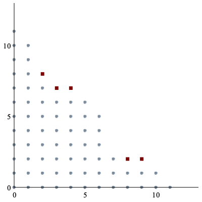
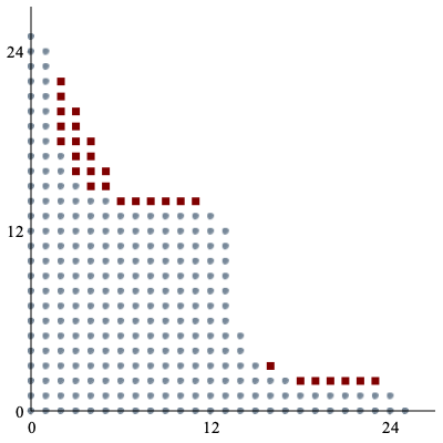
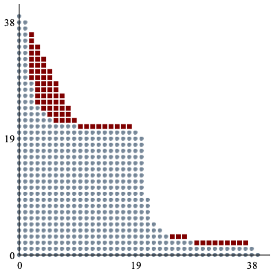
Figure 3.3: $\mathfrak{X}_{r}^{\mathcal{B}_{2}}$, for $r\in\{6,13,20\}$ : the elements that do not belong to $\mathcal{C}_{r}^{2}+\mathcal{C}_{r}^{2}+\mathcal{C}_{2}^{2}$ are represented by carmin squares.

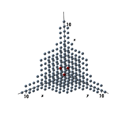
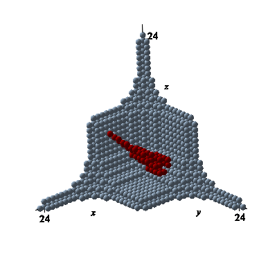
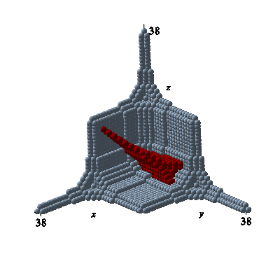
Figure 3.4: $\mathfrak{X}_{r}^{\mathcal{A}_{3}}$, for $r\in\{6,13,20\}$ : the elements in purple do not belong to $\mathcal{C}_{r}^{3}+\mathcal{C}_{r}^{3}+\mathcal{C}_{2}^{3}$.

4 Support of a linear form on the Laurent polynomial ring

In Section 3 we converted the recovery of the support of a polynomial in the monomial or Chebyshev bases to the recovery of the support of a linear form. For

$$f(x)=\sum_{i=1}^{r}a_{i}x^{\beta_{i}},\qquad F(X)=\sum_{i=1}^{r}a_{i}\,T_{\beta_{i}}(X),\quad\hbox{ or }\quad F(X)=\sum_{i=1}^{r}a_{i}\,U_{\beta_{i}}(X)$$

we respectively introduced the linear forms on $\mathbb{K}[x^{\pm}]$

$$\Omega=\sum_{i=1}^{r}a_{i}\mathbbm{e}_{\zeta_{i}},\qquad\sum_{i=1}^{r}a_{i}\sum_{A\in\mathcal{W}}\mathbbm{e}_{A\star\zeta_{i}},\quad\hbox{ or }\quad\sum_{i=1}^{r}a_{i}\sum_{A\in\mathcal{W}}\det(A)\,\mathbbm{e}_{A\star\zeta_{i}}$$

where, for some chosen $\xi\in\mathbb{N}_{>0}$, $\zeta_{i}=\xi^{{\beta}_{i}^{{\mathsf{T}}}}$, $\zeta_{i}=\xi^{{\beta}_{i}^{{\mathsf{T}}}S}$, or $\zeta_{i}=\xi^{{(\delta+\beta_{i})}^{{\mathsf{T}}}S}$. The linear forms are known from their values at some polynomials, respectively:

$$\Omega(x^{\alpha})=f(\xi^{\alpha}),\quad\Omega({\Theta}_{\alpha})=F\left({\Theta}_{\omega_{1}}(\xi^{{\alpha}^{{\mathsf{T}}}S}),\ldots,{\Theta}_{\omega_{n}}(\xi^{{\alpha}^{{\mathsf{T}}}S})\right),$$

or

$$\Omega({\Upsilon}_{\alpha})={\Upsilon}_{\delta}\left(\xi^{{\alpha}^{{\mathsf{T}}}S}\right)\,F\left({\Theta}_{\omega_{1}}\left(\xi^{{\alpha}^{{\mathsf{T}}}S}\right),\ldots,{\Theta}_{\omega_{n}}(\xi^{{\alpha}^{{\mathsf{T}}}S})\right).$$

This section provides the technology to recover the support of these linear forms. We shall either retrieve

$$\left\{\zeta_{1},\,\ldots,\zeta_{r}\right\}\subset\mathbb{Q}^{n},\quad\hbox{ or }\quad\left\{\left({\Theta}_{\omega_{1}}(\zeta_{i}),\ldots,\,{\Theta}_{\omega_{n}}(\zeta_{i})\right)\;|\;1\leq i\leq r\right\}\subset\mathbb{N}^{n}$$

Identifying the support of a linear form on a polynomial ring $\mathbb{K}[x]$ already has applications in optimization, tensor decomposition and cubature [1, 2, 9, 13, 15, 36, 37]. How to take advantage of symmetry in some of these applications appears in [14, 21, 52]. To a linear form $\Omega:\mathbb{K}[x]\rightarrow\mathbb{K}$ one associates [13, 15, 45, 50] a Hankel operator $\widehat{\mathcal{H}}:\mathbb{K}[x]\rightarrow\mathbb{K}[x]^{*}$ whose kernel $I_{\Omega}$ is the ideal of the support $\left\{\zeta_{1},\,\ldots,\,\zeta_{n}\right\}$ of $\Omega$. We can compute directly these points as eigenvalues of the multiplication maps on the quotient algebra $\mathbb{K}[x]/I_{\Omega}$.

The present application to sparse interpolation is related to a multivariate version of Prony’s method, as tackled in [34, 45, 55]. Contrary to the previously mentioned applications, where the symmetry is given by the linear action of a finite group on the ambient space of the support, here the Weyl groups act linearly on $\mathbb{K}[x^{\pm}]$ but nonlinearly on the ambient space of the support. Thanks to Theorem 2.27, we can satisfy ourselves with recovering only the values of the freely generating invariant polynomials on the support, i.e. $\left\{\left({\Theta}_{\omega_{1}}(\zeta_{i}),\ldots,\,{\Theta}_{\omega_{n}}(\zeta_{i})\right)\;|\;1\leq i\leq r\right\}$.

In Section 4.1 we review the definitions of Hankel operators associated to a linear form, multiplication maps and their relationship to each other in the context of $\mathbb{K}[x^{\pm}]$ rather than $\mathbb{K}[x]$. In Section 4.2 we present an algorithm to calculate the matrix representation of certain multiplication maps and determine the support of the original linear form as eigenvalues of the multiplication maps. In Section 4.3, to retrieve the orbits forming the support of an invariant or semi-invariant form, we introduce the Hankel operators $\widehat{\mathcal{H}}:\mathbb{K}[x^{\pm}]^{\mathcal{W}}\rightarrow\left(\mathbb{K}[x^{\pm}]^{\mathcal{W}}_{\chi}\right)^{*}$, where $\mathbb{K}[x^{\pm}]^{\mathcal{W}}$ is the ring of invariants for the action of the Weyl group $\mathcal{W}$ on $\mathbb{K}[x^{\pm}]$; $\mathbb{K}[x^{\pm}]^{\mathcal{W}}_{\chi}$ is the $\mathbb{K}[x^{\pm}]^{\mathcal{W}}$-module of $\chi$-invariant polynomials where $\chi:\mathcal{W}\rightarrow\left\{1,-1\right\}$ is either given by $\chi(A)=1$ or $\chi(A)=\det A$, depending whether we consider Chebyshev polynomials of the first or second kind. In this latter section, in analogy to the previous sections, we also introduce the appropriate multiplication maps and give an algorithm to determine the support of the associated $\chi$-invariant linear from in terms of the eignevalues of these multiplication maps.

The construction could be extended to other group actions on the ring of (Laurent) polynomials. Yet we shall make use of the fact that, for a Weyl group $\mathcal{W}$, $\mathbb{K}[x^{\pm}]^{\mathcal{W}}$ is isomorphic to a polynomial ring and $\mathbb{K}[x^{\pm}]^{\mathcal{W}}_{\chi}$ is a free $\mathbb{K}[x^{\pm}]^{\mathcal{W}}$-module of rank one.

4.1 Hankel operators and multiplication maps

We consider a commutative $\mathbb{K}$-algebra $\mathcal{R}$ and a $\mathcal{R}$-module $\mathcal{S}$. $\mathcal{R}$ will later be either $\mathbb{K}[x^{\pm}]$ or the invariant subring $\mathbb{K}[x^{\pm}]^{\mathcal{W}}$ while $\mathcal{S}$ will be either $\mathbb{K}[x^{\pm}]$, $\mathbb{K}[x^{\pm}]^{\mathcal{W}}$ or ${\Upsilon}_{\delta}\mathbb{K}[x^{\pm}]^{\mathcal{W}}$, the module of skew-invariant polynomials (Lemma 2.21). Hence $\mathcal{S}$ shall be a free $\mathcal{R}$-modules of rank one: there is an element that we shall denote $\Upupsilon$ in $\mathcal{S}$ s.t. $\mathcal{S}=\Upupsilon\mathcal{R}$. In the cases of interest $\Upupsilon$ is either $1$ or ${\Upsilon}_{\delta}$. We shall keep the explicit mention of $\Upupsilon$ though the $\mathcal{R}$-module isomorphism between $\mathcal{R}$ and $\mathcal{S}$ would allow us to forego the use of $\mathcal{S}$.

$\mathcal{R}$ and $\mathcal{S}$ are also $\mathbb{K}$-vector spaces. To a $\mathbb{K}$-linear form $\Omega$ on $\mathcal{S}$ we associate a Hankel operator $\widehat{\mathcal{H}}:\mathcal{R}\rightarrow\mathcal{S}^{*}$, where $\mathcal{S}^{*}$ is the dual of $\mathcal{S}$, i.e. the $\mathbb{K}$-vector space of $\mathbb{K}$-linear forms on $\mathcal{S}$. The kernel of this operator is an ideal $I_{\Omega}$ in $\mathcal{R}$, considered as a ring. The matrices of the multiplication maps in $\mathcal{R}/I_{\Omega}$ are given in terms of the matrix of $\widehat{\mathcal{H}}$.

Hankel operator

For a linear form $\Omega\in\mathcal{S}^{*}$, the associated Hankel operator $\widehat{\mathcal{H}}$ is the $\mathbb{K}$-linear map

$$\widehat{\mathcal{H}}:\begin{array}[t]{ccc}\mathcal{R}&\to&\mathcal{S}^{*}\\ p&\mapsto&\Omega_{p},\end{array}\quad\hbox{ where }\quad\Omega_{p}:\begin{array}[t]{ccc}\mathcal{S}&\to&\mathbb{K}\\ q&\mapsto&\Omega(q\,p).\end{array}$$

If $U$ and $V$ are $\mathbb{K}$-linear subspaces of $\mathcal{R}$ and $\mathcal{S}$ respectively we define $\widehat{\mathcal{H}}_{|U,V}$ using the restrictions $\Omega_{p|V}$ of $\Omega_{p}$ to $V$:

$$\widehat{\mathcal{H}}_{|U,V}:\begin{array}[t]{ccc}U&\to&V^{*}\\ p&\mapsto&\Omega_{p|V},\end{array}$$

Assume $U$ is the $\mathbb{K}$-linear span $\left\langle B\right\rangle=\left\langle b_{1},\ldots,b_{r}\right\rangle$ of a linearly independent set $B=\left\{b_{1},\ldots,b_{r}\right\}$ in $\mathcal{R}$ and $V$ is the $\mathbb{K}$-linear span $\left\langle\Upupsilon c_{1},\ldots,\Upupsilon c_{s}\right\rangle$ in $\mathcal{S}$, denoted $\left\langle\Upupsilon C\right\rangle$, where $C=\left\{c_{1},\ldots,c_{s}\right\}$ is a linearly independent subset of $\mathcal{R}$. Then the matrix of $\widehat{\mathcal{H}}_{|U,V}$ in $B$ and the dual basis of $\Upupsilon C$ is

$$H_{1}^{C,B}=\left(\Omega(\Upupsilon c_{i}\,b_{j})\right)_{\begin{subarray}{c}1\leq i\leq s\\ 1\leq j\leq r\end{subarray}}.$$

The kernel of $\widehat{\mathcal{H}}$

$$I_{\Omega}=\left\{p\in\mathcal{R}\;|\;\Omega_{p}=0\right\}=\left\{p\in\mathcal{R}\;|\;\Omega(q\,p)=0,\;\forall q\in\mathcal{S}\right\}$$

is an ideal of $\mathcal{R}$. We shall consider both the quotient spaces $\mathcal{R}/I_{\Omega}$ and $\mathcal{S}/\Upupsilon I_{\Omega}$ where $\Upupsilon I_{\Omega}$ is the submodule $I_{\Omega}\mathcal{S}$ of $\mathcal{S}$.

Lemma 4.1

The image of $\widehat{\mathcal{H}}$ lies in $\left(\Upupsilon I_{\Omega}\right)^{\perp}$ and $\widehat{\mathcal{H}}$ induces an injective morphism $\mathcal{H}:\mathcal{R}/I_{\Omega}\rightarrow\left(\mathcal{S}/\Upupsilon I_{\Omega}\right)^{*}$ that has the following diagram commute.

Proof.

A basis of $\mathcal{R}/I_{\Omega}$ is the image by the natural projection $\pi:\mathcal{R}\rightarrow\mathcal{R}/I_{\Omega}$ of a linearly independent set $C\subset\mathcal{R}$ s.t. $\mathcal{R}=\left\langle C\right\rangle\oplus I_{\Omega}$. Hence $\mathcal{S}=\left\langle\Upupsilon C\right\rangle\oplus\Upupsilon I_{\Omega}$. Recall from linear algebra, see for instance [24, Proposition V, Section 2.30], that this latter equality implies:

$$\mathcal{S}^{*}=\left(\Upupsilon I_{\Omega}\right)^{\perp}\oplus\left(\Upupsilon C\right)^{\perp}\quad\hbox{ and }\quad\begin{array}[t]{ccc}\left(\Upupsilon I_{\Omega}\right)^{\perp}&\rightarrow&{\left\langle\Upupsilon C\right\rangle}^{*}\\ \Phi&\mapsto&\Phi_{|\left\langle\Upupsilon C\right\rangle}\end{array}\hbox{is an isomorphism,}$$

where, for any set $V\subset\mathcal{S}$, $\displaystyle V^{\perp}=\left\{\Phi\in\mathcal{S}^{*}\;|\;\Phi(v)=0,\forall v\in V\right\}$ is a $\mathbb{K}$-linear subspace of $\mathcal{S}^{*}$.

Note that the image of $\widehat{\mathcal{H}}$ lies in $\left(\Upupsilon I_{\Omega}\right)^{\perp}$. With the natural identification of $\left\langle\Upupsilon C\right\rangle^{*}$ with $\left(\mathcal{S}/\Upupsilon I_{\Omega}\right)^{*}$, the factorisation of $\widehat{\mathcal{H}}$ by the natural projection $\pi:\mathcal{R}\rightarrow\mathcal{R}/I_{\Omega}$ defines the injective morphism $\mathcal{H}:\mathcal{R}/I_{\Omega}\rightarrow\left(\mathcal{S}/\Upupsilon I_{\Omega}\right)^{*}$ through the announced commuting diagram.    $\Box$

If the rank of $\widehat{\mathcal{H}}$ is finite and equal to $r$, then the dimension of $\mathcal{R}/I_{\Omega}$, $\mathcal{S}/\Upupsilon I_{\Omega}$ and $\left(\mathcal{S}/\Upupsilon I_{\Omega}\right)^{*}$, as $\mathbb{K}$-vector spaces, is $r$ and the injective linear operator $\mathcal{H}$ is then an isomorphism. The point here is the following criterion for detecting bases of $\mathcal{R}/I_{\Omega}$.

Theorem 4.2

Assume that $\operatorname{rank}\widehat{\mathcal{H}}=r<\infty$ and consider $B=\{b_{1},\ldots,b_{r}\}$ and $C=\{c_{1},\ldots,c_{r}\}$ subsets of $\mathcal{R}$. Then the image of $B$ and $C$ by $\pi:\mathcal{R}\rightarrow\mathcal{R}/I_{\Omega}$ are both bases of $\mathcal{R}/I_{\Omega}$ if and only if the matrix $H_{1}^{C,B}$ is non-singular.

Proof.

Assume that $B$ and $C$ are both bases for $\mathcal{R}/I_{\Omega}$, we can identify $\mathcal{R}/I_{\Omega}$ with $\left\langle B\right\rangle$ and $\mathcal{S}/\Upupsilon I_{\Omega}$ with $\left\langle\Upupsilon C\right\rangle$. Hence $H_{1}^{C,B}$ is the matrix of $\mathcal{H}$ in the basis $B$ and the dual basis of $\Upupsilon C$. Since $\mathcal{H}$ is an isomorphism, $H_{1}^{C,B}$ is nonsingular.

Assume $H_{1}^{C,B}$ is nonsingular. We need to show that $B$ and $C$ are linearly independent modulo $I_{\Omega}$, i.e. that any linear combination of their elements that belongs to the ideal is trivial. Take $a=(a_{1},\dots,a_{r})\in\mathbb{K}^{r}$ such that $a_{1}b_{1}+\dots+a_{r}b_{r}\in I_{\Omega}$. Using the definition of $I_{\Omega}$, we get $a_{1}\Omega(\Upupsilon c_{i}\,b_{1})+\dots+a_{r}\Omega(\Upupsilon c_{i}\,b_{r})=0\quad\forall i=1,\dots,r$. These equalities amount to $H_{1}^{C,B}a=0$ and thus $a=0$. Similarly $a_{1}c_{1}+\dots+a_{r}c_{r}\equiv 0\mod I_{\Omega}$ leads to ${a}^{{\mathsf{T}}}H_{1}^{C,B}=0$ and hence $a=0$.    $\Box$

Multiplication maps

We now assume that the Hankel operator $\widehat{\mathcal{H}}$ associated to $\Omega$ has finite rank $r$. Then $\mathcal{R}/I_{\Omega}$ is of dimension $r$ when considered as a linear space over $\mathbb{K}$. For $p\in\mathcal{R}$, consider the multiplication map

$$\widehat{\mathcal{M}}_{p}:\begin{array}[t]{ccc}\mathcal{R}&\rightarrow&\mathcal{R}\\ q&\mapsto&q\,p\end{array}\quad\hbox{ and }\quad\mathcal{M}_{p}:\begin{array}[t]{ccl}\mathcal{R}/I_{\Omega}&\rightarrow&\mathcal{R}/I_{\Omega}\\ q^{\prime}&\mapsto&\pi(q\,p)\hbox{ where }q\in\mathcal{R}\hbox{ satisfies }\pi(q)=q^{\prime}.\end{array}\;$$ (4.1)

${\mathcal{M}}_{p}$ is a well defined linear map respecting the following commuting diagram [17, Proposition 4.1]
                                       

Let us temporarily introduce the Hankel operator $\widehat{\mathcal{H}}_{p}$ associated to $\Omega_{p}$. This is the map defined by $\widehat{\mathcal{H}}_{p}=\widehat{\mathcal{H}}\circ\widehat{\mathcal{M}}_{p}$. Therefore the image of $\widehat{\mathcal{H}}_{p}$ is included in the image of $\widehat{\mathcal{H}}$ and $\ker\widehat{\mathcal{H}}\subset\ker\widehat{\mathcal{H}}_{p}$. We can thus construct the maps $\mathcal{H}_{p}$ that satisfy $\widehat{\mathcal{H}}_{p}=\mathcal{H}_{p}\circ\pi$. Then $\mathcal{H}_{p}=\mathcal{H}\circ\mathcal{M}_{p}$ and we have the following commuting diagram.

Theorem 4.3

Assume the Hankel operator $\widehat{\mathcal{H}}$ associated to the linear form $\Omega$ has finite rank $r$. Let $B=\left\{b_{1},\,\ldots,\,b_{r}\right\}$ and $C=\left\{c_{1},\,\ldots,\,c_{r}\right\}$ be bases of $\mathcal{R}/I_{\Omega}$. Then the matrix $M_{p}^{B}$ of the multiplication by an element $p$ of $\mathcal{R}$ in $\mathcal{R}/I_{\Omega}$ is given by

$$M_{p}^{B}=\left(H_{1}^{C,B}\right)^{-1}\,H_{p}^{C,B}\quad\hbox{ where }\quad H_{1}^{C,B}=\left(\Omega(\Upupsilon c_{i}\,b_{j})\right)_{1\leq i,j\leq r}\;\hbox{ and }\;H_{p}^{C,B}=\left(\Omega(\Upupsilon c_{i}\,b_{j}\,p)\right)_{1\leq i,j\leq r}$$

Proof.

The matrix of $\mathcal{H}_{p}$ in $B$ and the dual basis of $\Upupsilon C$ is $H_{p}^{C,B}$. Then $H_{p}^{C,B}=H_{1}^{C,B}\,M_{p}^{B}$ since $\mathcal{H}_{p}=\mathcal{H}\circ\mathcal{M}_{p}$. From Theorem 4.2, $H_{1}^{C,B}$ is invertible.    $\Box$

4.2 Support of a linear form on $\mathbb{K}[x^{\pm}]$

We now consider $\mathcal{R}$ and $\mathcal{S}$ to be the ring of Laurent polynomials $\mathbb{K}[x^{\pm}]$. As before, the evaluations $\mathbbm{e}_{\zeta}:\mathbb{K}[x^{\pm}]\rightarrow\mathbb{K}$ at a point $\zeta\in\left({\mathbb{K}}^{*}\right)^{n}$ are defined as follow: For $p\in\mathbb{K}[x^{\pm}]$, $\mathbbm{e}_{\zeta}(p)=p(\zeta)$. For $a_{1},\,\ldots,\,a_{r}\in{\mathbb{K}}^{*}$ and distinct $\zeta_{1},\,\ldots,\,\zeta_{r}\in({\mathbb{K}}^{*})^{n}$ we write $\Omega=\sum_{i=1}^{r}a_{i}\,\mathbbm{e}_{\zeta_{i}}$ for the linear form

$$\Omega:\begin{array}[t]{ccc}\mathbb{K}[x^{\pm}]&\rightarrow&\mathbb{K}\\ p&\mapsto&\displaystyle\sum_{i=1}^{r}a_{i}\,p(\zeta_{i}).\end{array}$$

In this section we characterize such a linear form in terms of its associated Hankel operator. We show how to compute $\zeta_{1},\,\ldots,\,\zeta_{r}$ from the knowledge of the values of $\Omega$ on a finite dimensional subspace of $\mathbb{K}[x^{\pm}]$.

4.2.1 Determining a basis of the quotient algebra

Theorem 4.4

If $\displaystyle\Omega=\sum_{i=1}^{r}a_{i}\,\mathbbm{e}_{\zeta_{i}}$, where $a_{i}\in{\mathbb{K}}^{*}$, and $\zeta_{1},\,\ldots,\,\zeta_{r}$ are distinct points in $({\mathbb{K}}^{*})^{n}$ then the associated Hankel operator $\widehat{\mathcal{H}}$ has finite rank $r$ and its kernel $I_{\Omega}$ is the annihilating ideal of $\left\{\zeta_{1},\,\ldots,\zeta_{r}\right\}$.

Proof.

It is easy to see that $p(\zeta_{1})=\ldots=p(\zeta_{r})=0$ implies that $p\in I_{\Omega}$. For the converse inclusion, consider some interpolation polynomials $p_{1},\,\ldots,\,p_{r}$ at $\zeta_{1},\,\ldots,\,\zeta_{r}$, i.e. $p_{i}(\zeta_{i})=1$ and $p_{j}(\zeta_{i})=0$ when $i\neq j$ [17, Lemma 2.9]. For $q\in I_{\Omega}$ we have $\Omega(q\,p_{i})=0$ and thus $a_{i}\,q(\zeta_{i})=0$. Hence $I_{\Omega}$ is the annihilating ideal of $\left\{\zeta_{1},\,\ldots,\zeta_{r}\right\}$. It is thus a radical ideal with $\dim_{\mathbb{K}}\mathbb{K}[x^{\pm}]/I_{\Omega}=r$.    $\Box$

Theorem 4.2 gives necessary and sufficient condition for a set $B=\left\{b_{1},\ldots,b_{r}\right\}$ in $\mathbb{K}[x^{\pm}]$ to be a basis of $\mathbb{K}[x^{\pm}]/I_{\Omega}$ when the dimension of this latter, as a $\mathbb{K}$-vector space, is $r$. This condition is that the matrix $H_{1}^{B}=\left(\Omega(b_{i}b_{j})\right)_{1\leq i,j\leq r}$ is nonsingular. The problem of where to look for this basis was settled in [55] where the author introduces lower sets and the positive octant of the hypercross of order $r$.

A subset $\Gamma$ of $\mathbb{N}^{n}$ is a lower set if whenever $\alpha+\beta\in\Gamma$, $\alpha,\beta\in\mathbb{N}^{n}$, then $\alpha\in\Gamma$. The positive octant of the hypercross of order $r$ is

$$\mathcal{C}_{r}^{n}=\left\{\alpha\in\mathbb{N}^{n}\;\left|\;\prod_{i=1}^{r}(\alpha_{i}+1)\leq r\right.\right\}.$$

It is the union all the lower sets of cardinality $r$ or less [55, Lemma 10]. We extend [55, Corollary 11] for further use in Section 4.3.

Proposition 4.5

Let $\leqslant$ be an order on $\mathbb{N}^{n}$ such that $0\leqslant\gamma$ and $\alpha\leqslant\beta\Rightarrow\alpha+\gamma\leqslant\beta+\gamma$ for all $\alpha,\beta,\gamma\in\mathbb{N}^{n}$. Consider two families of polynomials $\left\{P_{\alpha}\,|\,\alpha\in\mathbb{N}^{n}\right\}$ and $\left\{Q_{\alpha}\,|\,\alpha\in\mathbb{N}^{n}\right\}$ in $\mathbb{K}[X]$ such that $P_{\alpha}=\sum_{\beta\leqslant\alpha}p_{\beta}X^{\beta}$ and $Q_{\alpha}=\sum_{\beta\leqslant\alpha}q_{\beta}X^{\beta}$ with $p_{\alpha},\,q_{\alpha}\neq 0$.

If $J$ is an ideal in $\mathbb{K}[X]=\mathbb{K}[X_{1},\ldots,X_{n}]$ such that $\dim_{\mathbb{K}}\mathbb{K}[X]/J=r$ then there exists a lower set $\Gamma$ of cardinal $r$ such that both $\left\{P_{\alpha}\,|\,\alpha\in\Gamma\right\}$ and $\left\{Q_{\alpha}\,|\,\alpha\in\Gamma\right\}$ are bases of $\mathbb{K}[X]/J$.

Proof.

For the chosen term order $\leqslant$, a Gröbner basis of $J$ defines a lower set $\Gamma$ that has $r$ monomials and is a basis of $\mathbb{K}[x]/J$ [17, Chapter 2].

Consider a polynomial $P=\sum_{\beta\in\Gamma}a_{\beta}P_{\beta}$, for some $a_{\beta}\in\mathbb{K}$ not all zero. Take $\alpha$ to be highest element of $\Gamma$ for which $a_{\alpha}\neq 0$. Then $X^{\alpha}$ is the leading term of $P$. As $X^{\alpha}$ does not belong to the initial ideal, $P\notin J$ [16, Chapter 2]. It follows that $\left\{P_{\alpha}\,|\,\alpha\in\Gamma\right\}$ is linearly independent modulo $J$ and hence is a basis of $\mathbb{K}[X]/J$. The same is applies to $\left\{Q_{\alpha}\,|\,\alpha\in\Gamma\right\}$.    $\Box$

Corollary 4.6

If $I$ is an ideal in $\mathbb{K}[x^{\pm}]$ such that $\dim_{\mathbb{K}}\mathbb{K}[x^{\pm}]/I=r$ then $\mathbb{K}[x^{\pm}]/I$ admits a basis in $\left\{x^{\alpha}\,|\,\alpha\in\mathcal{C}_{r}^{n}\right\}.$

Proof.

A monomial basis of $\mathbb{K}[x]/J$, where $J=I\cap\mathbb{K}[x]$, is a basis for $\mathbb{K}[x^{\pm}]/I$.    $\Box$

4.2.2 Eigenvalues and eigenvectors of the multiplication matrices

The eigenvalues of the multiplication map $\mathcal{M}_{p}$, introduced in Equation 4.1, are the values of $p$ on the variety of $I_{\Omega}$; as $I_{\Omega}$ is a radical ideal, this is part of the following result, which is a simple extension of [17, Chapter 2, Proposition 4.7 ] to the Laurent polynomial ring. The proof appears as a special case of the later Proposition 4.14.

Theorem 4.7

Let $I$ be a radical ideal in $\mathbb{K}[x^{\pm}]$ whose variety consists of $r$ distinct points $\zeta_{1},\,\ldots,\zeta_{r}$ in $(\bar{\mathbb{K}}^{*})^{n}$ then:

• A set $B=\left\{b_{1},\ldots,b_{r}\right\}$ is a basis of $\mathbb{K}[x^{\pm}]/I$ if and only if the matrix $W_{\zeta}^{B}=\left(b_{j}(\zeta_{i})\right)_{1\leq i,j\leq r}$ is non singular;

• The matrix $M_{p}^{B}$ of the multiplication $\mathcal{M}_{p}$ by $p$ in a basis $B$ of $\mathbb{K}[x^{\pm}]/I$ satisfies $W_{\zeta}^{B}\,M_{p}^{B}=D_{\zeta}^{p}\,W_{\zeta}^{B}$ where $D_{\zeta}^{p}$ is the diagonal matrix $\operatorname{diag}(p(\zeta_{1}),\,\ldots,\,p(\zeta_{r}))$.

This theorem gives us a basis of left eigenvectors for $M_{p}^{B}$: The $i$-th row of $W_{\zeta}^{B}$, $\begin{bmatrix}b_{1}(\zeta_{i})&\ldots&b_{r}(\zeta_{i})\end{bmatrix}$, is a left eigenvector associated to the eigenvalue $p(\zeta_{i})$. One can furthermore observe that

$$H_{1}^{C,B}={\left(W_{\zeta}^{C}\right)}^{{\mathsf{T}}}\,A\,W_{\zeta}^{B}\hbox{ where }A=\operatorname{diag}(a_{1},\ldots,a_{r}).$$ (4.2)

4.2.3 Algorithm

Assuming that a linear form $\Omega$ on $\mathbb{K}[x^{\pm}]$ is a weighted sum of evaluations at some points of $({\mathbb{K}}^{*})^{n}$, we wish to determine its support and its coefficients. We assume we know the cardinal $r$ of this support and that we can evaluate $\Omega$ at the monomials $\left\{x^{\alpha}\right\}_{\alpha\in\mathbb{N}^{n}}$. In other words, we assume that $\Omega=\sum_{i=1}^{r}a_{i}\mathbbm{e}_{\zeta_{i}}$ where $\zeta_{1},\,\ldots,\,\zeta_{r}\in({\mathbb{K}}^{*})^{n}$ and then $a_{1},\ldots,a_{r}\in{\mathbb{K}}^{*}$ are the unknowns. For that we have access as input to $\left\{\Omega\left(x^{\alpha+\beta+\gamma}\right)|\alpha,\beta\in\mathcal{C}_{r}^{n};|\gamma|\leq 1\right\}$.

The ideal $I_{\Omega}$ of these points is the kernel of the Hankel operator associated to $\Omega$. One strategy would consist in determining a set of generators, or even a Gröbner basis, of this ideal and then find its roots with a method to be chosen. In the present case there is nonetheless the possibility to directly form the matrices of the multiplication maps in $\mathbb{K}[x^{\pm}]/I_{\Omega}$ (applying Theorem 4.3) once a basis for $\mathbb{K}[x^{\pm}]/I_{\Omega}$ is determined (applying Theorem 4.2 and Corollary 4.6). The key fact that is used is that the set of $j^{th}$ coordinates of the $\zeta_{i}$, $\{\zeta_{1,j},\ldots,\zeta_{r,j}\}$, are the left eigenvalues of the multiplication map $\mathcal{M}_{x_{j}}:\mathbb{K}[x^{\pm}]/I_{\Omega}\rightarrow\mathbb{K}[x^{\pm}]/I_{\Omega}$, where $\mathcal{M}_{x_{j}}(\overline{p})=\overline{x_{j}}\overline{p}$. The matrices of these maps commute and are simultaneously diagonalizable (Theorem 4.7 or [16, Chapter 2, §4, Exercise 12]). One could calculate the eigenspaces of the first matrix and proceed by induction to give such a common diagonalization since these eigenspaces are left invariant by the other matrices. A more efficient approach given in the algorithm is to take a generic linear combination of these matrices that ensures that this new matrix has distinct eigenvalues and calculate a basis of eigenvectors for it. In this basis each of the original matrices is diagonal.

Algorithm 4.8

Support & Coefficients

Input: $r\in\mathbb{N}_{>0}$ and $\left\{\Omega\left(x^{\gamma+\alpha+\beta}\right)\;|\;\alpha,\beta\in\mathcal{C}_{r}^{n},\,|\gamma|\leq 1\right\}$

Output:

• The points $\zeta_{i}=\left[\zeta_{i,1},\,\ldots,\,\zeta_{i,n}\right]\in\mathbb{K}^{n}$, for $1\leq i\leq r$,

• The vector $\left[a_{1},\ldots,a_{r}\right]\in({\mathbb{K}}^{*})^{n}$ of coefficients,

such that $\displaystyle\Omega=\sum_{i=1}^{r}a_{i}\mathbbm{e}_{\zeta_{i}}$.

• Form the matrix $H_{0}^{\mathcal{C}_{r}^{n}}=\left[\Omega\left(x^{\alpha+\beta}\right)\right]_{\alpha,\beta\in\mathcal{C}_{r}^{n}}$

• Determine a lower set $\Gamma$ within $\mathcal{C}_{r}^{n}$ of cardinal $r$ such that the principal submatrix $H_{0}^{\Gamma}$ indexed by $\Gamma$ is nonsingular.

  % $\Gamma=\left\{0,\,\gamma_{2},\,\ldots,\,\gamma_{r}\right\}$ and $\left\{x^{\gamma}\,|\,\gamma\in\Gamma\right\}$ is a basis of $\mathbb{K}[x^{\pm}]/I_{\Omega}$ (Theorem 4.2).

• Form the matrices $H_{j}^{\Gamma}=\left[\Omega\left(x_{j}\,x^{\alpha+\beta}\right)\right]_{\alpha,\beta\in\Gamma}$ and the matrices $M_{j}^{\Gamma}=\left(H_{1}^{\Gamma}\right)^{-1}H_{j}^{\Gamma}$, for $1\leq j\leq n$.

  % $M_{j}^{\Gamma}$ is the matrix of multiplication by $x_{j}$ in $\mathbb{K}[x^{\pm}]/I_{\Omega}$ (Theorem 4.3)
  % The matrices $M_{1}^{\Gamma},\,\ldots,\,M_{n}^{\Gamma}$ are simultaneously diagonalisable (Theorem 4.7).

• Consider $L=\ell_{1}M_{1}+\ldots+\ell_{n}M_{n}$ a generic linear combination of $M_{1},\,\ldots,\,M_{n}$

  % The eigenvalues of $L$ are $\lambda_{i}=\sum_{j=1}^{n}\ell_{j}\zeta_{i,j}$, for $1\leq i\leq r$. For most $\left[{\ell}_{1},\,\ldots,\,{\ell}_{n}\right]\in\mathbb{K}^{n}$ they are distinct.

• Compute $W$ a matrix whose rows are $r$ linearly independent left eigenvectors of $L$ appropriately nomalized

  % A left eigenvector associated to $\lambda_{i}$ is a nonzero multiple of the row vector $\left[1,(\zeta_{i})^{\gamma_{2}},\ldots,(\zeta_{i})^{\gamma_{r}}\right]$ (Theorem 4.7)
  % The normalization of the first component to $1$ allows us to assume the rows of $W$ are exactly these vectors.

• For $1\leq j\leq n$, determine the matrix $D_{j}=\operatorname{diag}(\zeta_{1,j},\,\ldots,\,\zeta_{r,j})$ such that $WM_{x_{j}}^{\Gamma}=D_{j}W$.

• For $1\leq i\leq r$, form the points $\zeta_{i}=\left[\zeta_{i,1},\,\ldots,\,\zeta_{i,n}\right]$ from the diagonal entries of the matrices $D_{j}$, $1\leq j\leq n$.

• Determine the matrix $\operatorname{diag}(a_{1},\ldots,a_{r})$ such that $H_{0}^{\Gamma}={W}^{{\mathsf{T}}}AW$.

  % Only the first row of the left and right handside matrices need to be considered,
  % resulting in the linear system $\displaystyle\begin{bmatrix}a_{1}&\ldots&a_{r}\end{bmatrix}W=\begin{bmatrix}\Omega(1)&\Omega(x^{\gamma_{2}})\ldots&\Omega(x^{\gamma_{r}})\end{bmatrix}$

Depending on the elements of $\Gamma$ it might be possible to retrieve the coordinates of the points $\zeta_{j}$ directly from $W$. The easiest case is when ${[1,\,0\,\ldots,\,0]}^{{\mathsf{T}}},\,\ldots,\,{[0\,\ldots,\,0,\,1]}^{{\mathsf{T}}}\in\Gamma$ : the coordinates of $\zeta_{j}$ can be read directly from the normalized left eigenvectors of $L$, i.e. the rows of $W$.

The determination of a lower set $\Gamma$ of cardinality $r$ whose associated principal submatrix is not singular is actually an algorithmic subject on its own. It is strongly tied to determining the Gröbner bases of $I_{\Omega}$ and is the focus of, for instance, [10, 54]. In a complexity meticulous approach to the problem, one would not form the matrix $H_{0}^{\mathcal{C}_{r}^{n}}$ at once, but construct $\Gamma$ and the associated submatrix degree by degree or following some term order. The number of evaluations of the function to interpolate is then reduced. This actual number of evaluation heavily depends on the shape of $\Gamma$.

Example 4.9

In Example 3.2 we called on Algorithm 4.8 with $r=2$ and

$$\Omega\left(x^{\gamma_{1}}y^{\gamma_{2}}\right)=f\left(\xi^{\gamma_{1}},\xi^{\gamma_{2}}\right)=a\,\xi^{\alpha_{1}\gamma_{1}+\alpha_{2}\gamma_{2}}+b\,\xi^{\beta_{1}\gamma_{1}+\beta_{2}\gamma_{2}}.$$

Hence

$$H_{0}^{\mathcal{C}_{2}^{2}}=\begin{bmatrix}f(\xi^{0},\xi^{0})&f(\xi^{1},\xi^{0})&f(\xi^{0},\xi^{1})\\ f(\xi^{1},\xi^{0})&f(\xi^{2},\xi^{0})&f(\xi^{1},\xi^{1})\\ f(\xi^{0},\xi^{1})&f(\xi^{1},\xi^{1})&f(\xi^{0},\xi^{2})\end{bmatrix}=\begin{bmatrix}a+b&a\xi^{\alpha_{1}}+b\xi^{\beta_{1}}&a\xi^{\alpha_{2}}+b\xi^{\beta_{2}}\\ a\xi^{\alpha_{1}}+b\xi^{\beta_{1}}&a\xi^{2\alpha_{1}}+b\xi^{2\beta_{1}}&a\xi^{\alpha_{1}+\alpha_{2}}+b\xi^{\beta_{1}+\beta_{2}}\\ a\xi^{\alpha_{2}}+b\xi^{\beta_{2}}&a\xi^{\alpha_{1}+\alpha_{2}}+b\xi^{\beta_{1}+\beta_{2}}&a\xi^{2\alpha_{2}}+b\xi^{2\beta_{2}}\end{bmatrix}$$

The lower sets of cardinality 2 are $\Gamma_{1}=\left\{{\begin{bmatrix}0&0\end{bmatrix}}^{{\mathsf{T}}},\,{\begin{bmatrix}1&0\end{bmatrix}}^{{\mathsf{T}}}\right\}$ and $\Gamma_{2}=\left\{{\begin{bmatrix}0&0\end{bmatrix}}^{{\mathsf{T}}},\,{\begin{bmatrix}0&1\end{bmatrix}}^{{\mathsf{T}}}\right\}$. One can check that the determinant of $H_{0}^{\mathcal{C}_{2}^{2}}$ is zero while the determinants of the principal submatrices indexed by $\Gamma_{1}$ and $\Gamma_{2}$ are respectively $ab(\xi^{\alpha_{1}}-\xi^{\beta_{1}})^{2}$ and $ab(\xi^{\alpha_{2}}-\xi^{\beta_{2}})^{2}$. Hence, whenever $\alpha_{1}\neq\beta_{1}$, $\Gamma_{1}$ is a valid choice, i.e. $H_{0}^{\Gamma_{1}}$ is non singular. Similarly for $\Gamma_{2}$ when $\alpha_{2}\neq\beta_{2}$.

Let us assume we can take $\Gamma=\Gamma_{1}$. We form:

$$H_{0}^{\Gamma}=\begin{bmatrix}f(\xi^{0},\xi^{0})&f(\xi^{1},\xi^{0})\\ f(\xi^{1},\xi^{0})&f(\xi^{2},\xi^{0})\end{bmatrix}=\begin{bmatrix}a+b&a\xi^{\alpha_{1}}+b\xi^{\beta_{1}}\\ a\xi^{\alpha_{1}}+b\xi^{\beta_{1}}&a\xi^{2\alpha_{1}}+b\xi^{2\beta_{1}}\end{bmatrix},$$

$$H_{1}^{\Gamma}=\begin{bmatrix}f(\xi^{1},\xi^{0})&f(\xi^{2},\xi^{0})\\ f(\xi^{2},\xi^{0})&f(\xi^{3},\xi^{0})\end{bmatrix}=\begin{bmatrix}a\xi^{\alpha_{1}}+b\xi^{\beta_{1}}&a\xi^{2\alpha_{1}}+b\xi^{2\beta_{1}}\\ a\xi^{2\alpha_{1}}+b\xi^{2\beta_{1}}&a\xi^{3\alpha_{1}}+b\xi^{3\beta_{1}}\end{bmatrix},$$

and

$$H_{2}^{\Gamma}=\begin{bmatrix}f(\xi^{0},\xi^{1})&f(\xi^{1},\xi^{1})\\ f(\xi^{1},\xi^{1})&f(\xi^{2},\xi^{1})\end{bmatrix}=\begin{bmatrix}a\xi^{\alpha_{2}}+b\xi^{\beta_{2}}&a\xi^{\alpha_{1}+\alpha_{2}}+b\xi^{\beta_{1}+\beta_{2}}\\ a\xi^{\alpha_{1}+\alpha_{2}}+b\xi^{\beta_{1}+\beta_{2}}&a\xi^{2\alpha_{1}+\beta_{2}}+b\xi^{2\beta_{1}+\beta_{2}}\end{bmatrix}.$$

It follows that the multiplication matrices are:

$$M_{1}=\left(H_{0}^{\Gamma}\right)^{-1}H_{1}^{\Gamma}=\begin{bmatrix}0&-\xi^{\alpha_{1}+\beta_{1}}\\ 1&\xi^{\alpha_{1}}+\xi^{\beta_{1}}\end{bmatrix}\hbox{ and }M_{2}=\left(H_{0}^{\Gamma}\right)^{-1}H_{2}^{\Gamma}=\begin{bmatrix}\displaystyle\frac{\xi^{\alpha_{1}+\beta_{2}}-\xi^{\alpha_{2}+\beta_{1}}}{\xi^{\alpha_{1}}-\xi^{\beta_{1}}}&\displaystyle-\xi^{\alpha_{1}+\beta_{1}}\frac{\xi^{\alpha_{2}}-\xi^{\beta_{2}}}{\xi^{\alpha_{1}}-\xi^{\beta_{1}}}\\ \displaystyle\frac{\xi^{\alpha_{2}}-\xi^{\beta_{2}}}{\xi^{\alpha_{1}}-\xi^{\beta_{1}}}&\displaystyle\frac{\xi^{\alpha_{1}+\alpha_{2}}-\xi^{\beta_{1}+\beta_{2}}}{\xi^{\alpha_{1}}-\xi^{\beta_{1}}}\end{bmatrix}.$$

The matrix of common left eigenvectors of $M_{1}$ and $M_{2}$, with only $1$ in the first column, is $\displaystyle W=\begin{bmatrix}1&\xi^{\alpha_{1}}\\ 1&\xi^{\beta_{1}}\end{bmatrix}.$ The diagonal matrices of eigenvalues are $\displaystyle D_{1}=\operatorname{diag}(\xi^{\alpha_{1}},\xi^{\beta_{1}})$ and $\displaystyle D_{2}=\operatorname{diag}(\xi^{\alpha_{2}},\xi^{\beta_{2}}).$ We shall thus output the points ${\left[\xi^{\alpha_{1}},\xi^{\alpha_{2}}\right]}^{{\mathsf{T}}}$ and ${\left[\xi^{\beta_{1}},\xi^{\beta_{2}}\right]}^{{\mathsf{T}}}$ of $\mathbb{K}^{2}$.

The first row of $H_{0}^{\Gamma}$ is $\begin{bmatrix}a&b\end{bmatrix}W$ so that the vector of coefficients $\begin{bmatrix}a&b\end{bmatrix}$ can be retrieved by solving the related linear system.

4.3 The case of $\chi$-invariant linear forms

We now consider $\mathcal{R}=\mathbb{K}[x^{\pm}]^{\mathcal{W}}$ and $\mathcal{S}=\mathbb{K}[x^{\pm}]^{\mathcal{W}}_{\chi}$ where $\mathcal{W}$ is a Weyl group acting on $\mathbb{K}[x^{\pm}]$ according to 2.1. The group morphism $\chi:\mathcal{W}\rightarrow\{1,-1\}$ is given by either $\chi(A)=1$ or $\chi(A)=\det(A)$. $\mathbb{K}[x^{\pm}]^{\mathcal{W}}_{\chi}$ is a free $\mathbb{K}[x^{\pm}]^{\mathcal{W}}$-module of rank one. When $\chi(A)=\det(A)$ a basis for it is ${\Upsilon}_{\delta}$ (Proposition 2.21). We may write $\mathbb{K}[x^{\pm}]^{\mathcal{W}}_{\chi}=\Upupsilon\mathbb{K}[x^{\pm}]^{\mathcal{W}}$ where $\Upupsilon$ can be $1$ or ${\Upsilon}_{\delta}$.

4.3.1 Restriction to the invariant ring

The starting point is a linear form $\Omega$ on $\mathbb{K}[x^{\pm}]$ that is $\chi$-invariant, i.e. $\Omega(A\cdot p)=\chi(A)\,\Omega(p)$ for all $A\in\mathcal{W}$ and $p\in\mathbb{K}[x^{\pm}]$. We show how the restricted Hankel operator

$$\widehat{\mathcal{H}}:\mathbb{K}[x^{\pm}]^{\mathcal{W}}\rightarrow\mathbb{K}[x^{\pm}]^{\mathcal{W}}_{\chi}$$

allows one to recover the orbits in the support of the $\chi$-invariant form

$$\Omega=\sum_{i=1}^{r}a_{i}\sum_{A\in\mathcal{W}}\chi(A)\,\mathbbm{e}_{A\star\zeta_{i}}$$

where the $\zeta_{i}\in({\mathbb{K}}^{*})^{n}$ have distinct orbits. By that we mean that we shall retrieve the values of the invariant polynomials ${\Theta}_{\omega_{1}},\ldots,{\Theta}_{\omega_{n}}$ on $\left\{\zeta_{1},\ldots,\,\zeta_{n}\right\}$.

The linear map

$$\mathfrak{p}_{\chi}:\begin{array}[t]{ccc}\mathbb{K}[x^{\pm}]&\rightarrow&\mathbb{K}[x^{\pm}]^{\mathcal{W}}_{\chi}\\ q&\mapsto&\displaystyle\frac{1}{|\mathcal{W}|}\sum_{A\in\mathcal{W}}\chi(A)^{-1}\,A\cdot q\end{array}$$

is a projection that satisfies

• $\mathfrak{p}_{\chi}(p\,q)=p\,\mathfrak{p}_{\chi}(q)$ for all $p\in\mathbb{K}[x^{\pm}]^{\mathcal{W}}$, $q\in\mathbb{K}[x^{\pm}]$, and

• $\mathfrak{p}_{\chi}(A\cdot q)=\chi(A)\,\mathfrak{p}_{\chi}(q)$ for all $q\in\mathbb{K}[x^{\pm}]$.

Then, for any $\chi$-invariant form $\Omega$ we have $\displaystyle\Omega(p)=\Omega\left(\mathfrak{p}_{\chi}(p)\right)$. Hence $\Omega$ is fully determined by its restriction to $\mathbb{K}[x^{\pm}]^{\mathcal{W}}_{\chi}$. We shall write $\Omega^{\mathcal{W}}$ when we consider the restriction of $\Omega$ to $\mathbb{K}[x^{\pm}]^{\mathcal{W}}_{\chi}$. Similarly, we denote $\widehat{\mathcal{H}}^{\mathcal{W}}$ and $I_{\Omega}^{\mathcal{W}}$ the Hankel operator associated to $\Omega^{\mathcal{W}}$ and its kernel. Hence $\widehat{\mathcal{H}}^{\mathcal{W}}:\mathbb{K}[x^{\pm}]^{\mathcal{W}}\rightarrow\left(\mathbb{K}[x^{\pm}]^{\mathcal{W}}_{\chi}\right)^{*}$ and $I_{\Omega}^{\mathcal{W}}$ is an ideal of $\mathbb{K}[x^{\pm}]^{\mathcal{W}}$.

Lemma 4.10

If $\displaystyle\Omega=\sum_{i=1}^{r}a_{i}\sum_{A\in\mathcal{W}}\chi(A)\,\mathbbm{e}_{A\star\zeta_{i}}$ then $\displaystyle I_{\Omega}^{\mathcal{W}}=I_{\Omega}\cap\mathbb{K}[x^{\pm}]^{\mathcal{W}}$ and the dimension of $\mathbb{K}[x^{\pm}]^{\mathcal{W}}/I_{\Omega}^{\mathcal{W}}$ is $r$.

Proof.

Take $p\in I_{\Omega}^{\mathcal{W}}\subset\mathbb{K}[x^{\pm}]^{\mathcal{W}}$. One wishes to show that for any $q\in\mathbb{K}[x^{\pm}]$ we have $\Omega(p\,q)=0$. This is true because $\Omega(p\,q)=\Omega(\mathfrak{p}_{\chi}(p\,q))=\Omega(p\,\mathfrak{p}_{\chi}(q))$ and $\Omega(p\,q^{\prime})=0$ for any $q^{\prime}\in\mathbb{K}[x^{\pm}]^{\mathcal{W}}$. Hence $I_{\Omega}^{\mathcal{W}}\subset I_{\Omega}\cap\mathbb{K}[x^{\pm}]^{\mathcal{W}}$. The other inclusion is obvious.

The proof that $\dim\mathbb{K}[x^{\pm}]^{\mathcal{W}}/I_{\Omega}^{\mathcal{W}}=r$ follows the structure of [17, Ch.2,Proposition 2.10]. Let $Z=\{A\star\zeta_{i}\ |\ A\in\mathcal{W},\;1\leq i\leq r\}$ be the union of the orbits of the $\zeta_{i}$. According to [17, Lemma 2.9], for each $i$ there exists a polynomial $\tilde{p}_{i}$ such that for $z\in Z$

$$\tilde{p}_{i}(z)=\left\{\begin{array}[]{ll}1&\hbox{ if }z=\zeta_{i}\\ 0&\hbox{ otherwise. }\end{array}\right.$$

Let $\mathcal{W}_{i}$ be the stabilizer of $\zeta_{i}$. Note that for $A\in\mathcal{W}$, $\tilde{p}_{i}(A\star\zeta_{j})=0$ if $j\neq i$ and $\tilde{p}_{i}(A\star\zeta_{i})=1$ if and only if $A\in\mathcal{W}_{i}$ . Define $p_{i}=\frac{|\mathcal{W}|}{|\mathcal{W}_{i}|}\,\mathfrak{p}_{1}(\tilde{p}_{i})$. We have $p_{i}\in\mathbb{K}[x^{\pm}]^{\mathcal{W}}$ and $p_{i}(\zeta_{j})=\delta_{i,j}$. Hence the linear map

$$\begin{array}[]{cccl}\phi~{}:&\mathbb{K}[x^{\pm}]^{\mathcal{W}}&\rightarrow&\mathbb{K}^{r}\\ &q&\mapsto&\begin{bmatrix}q(\zeta_{1})&\ldots&q(\zeta_{r})\end{bmatrix}\end{array}$$

is onto. We proceed to determine its kernel.

One easily sees that $I_{\Omega}\cap\mathbb{K}[x^{\pm}]^{\mathcal{W}}\subset\ker\phi$. Consider $q\in\ker\phi$. Since $q$ is invariant $q(A\star\zeta_{i})=q(\zeta_{i})=0$ for all $A\in\mathcal{W}$. By Theorem 4.4, $I_{\Omega}$ is the annihilating ideal of $\left\{A\textasteriskcentered\zeta_{i}\,|\,1\leq i\leq r,\;A\in\mathcal{W}/\mathcal{W}_{\zeta_{i}}\right\}$. Hence $q\in I_{\Omega}\cap\mathbb{K}[x^{\pm}]^{\mathcal{W}}$. Since $I_{\Omega}^{\mathcal{W}}=I_{\Omega}\cap\mathbb{K}[x^{\pm}]^{\mathcal{W}}$, we have proved that $\ker\phi=I_{\Omega}^{\mathcal{W}}$. Hence $\mathbb{K}[x^{\pm}]^{\mathcal{W}}/I_{\Omega}^{\mathcal{W}}$ is isomorphic to $\mathbb{K}^{r}$.    $\Box$

Theorem 4.11

If $\displaystyle\Omega=\sum_{i=1}^{r}a_{i}\sum_{A\in\mathcal{W}}\chi(A)\,\mathbbm{e}_{A\star\zeta_{i}}$, where $a_{i}\in{\mathbb{K}}^{*}$ and $\zeta_{1},\,\ldots,\,\zeta_{r}$ have distinct orbits in $({\mathbb{K}}^{*})^{n}$, then the Hankel operator $\widehat{\mathcal{H}}^{\mathcal{W}}$ associated to $\Omega^{\mathcal{W}}$ is of rank $r$. The variety of the extension of $I_{\Omega}^{\mathcal{W}}$ to $\mathbb{K}[x^{\pm}]$ is $\left\{A\star\zeta_{i}\;|\;A\in\mathcal{W},\;1\leq i\leq r\right\}$.

Proof.

Follows from Lemma 4.10 and Theorem 4.4.    $\Box$

4.3.2 Determining a basis of the quotient algebra

$\mathbb{K}[x^{\pm}]^{\mathcal{W}}$ is isomorphic to a polynomial ring $\mathbb{K}[X]=\mathbb{K}[X_{1},\ldots,X_{n}]$ (Proposition 2.11). Then Proposition 4.5 implies the following.

Corollary 4.12

Let $I^{\mathcal{W}}$ be an ideal of $\mathbb{K}[x^{\pm}]^{\mathcal{W}}$ such that the dimension of $\mathbb{K}[x^{\pm}]^{\mathcal{W}}/I^{\mathcal{W}}$ is of dimension $r$ as a $\mathbb{K}$-linear space. There exists a lower set $\Gamma$ of cardinal $r$ such that $\left\{{\Theta}_{\alpha}\;|\;\alpha\in\Gamma\right\}$ and $\left\{{\Xi}_{\alpha}\;|\;\alpha\in\Gamma\right\}$ are both bases of $\mathbb{K}[x^{\pm}]^{\mathcal{W}}/I^{\mathcal{W}}$.

Proof.

The Chebyshev polynomials of the first and second kind, $\left\{T_{\alpha}\right\}_{\alpha}$ and $\left\{U_{\alpha}\right\}_{\alpha}$, were defined in Definition 2.3 and 2.4 as the (only) polynomials in $\mathbb{K}[X]=\mathbb{K}[X_{1},\ldots,X_{n}]$ such that $T_{\alpha}({\Theta}_{\omega_{1}},\ldots,{\Theta}_{\omega_{2}})={\Theta}_{\alpha}$ and $U_{\alpha}({\Theta}_{\omega_{1}},\ldots,{\Theta}_{\omega_{2}})={\Xi}_{\alpha}$.

Consider $J$ the ideal in $\mathbb{K}[X]$ that corresponds to $I^{\mathcal{W}}$ through the isomorphism between $\mathbb{K}[x^{\pm}]^{\mathcal{W}}$ and $\mathbb{K}[X]$. Then $\dim_{\mathbb{K}}\mathbb{K}[X]/J=r$. With the order $\leq$ on $\mathbb{N}^{n}$ defined in Proposition 2.24, and by Proposition 2.23, $\left\{T_{\alpha}\right\}_{\alpha}$ and $\left\{U_{\alpha}\right\}_{\alpha}$ satisfy the hypothesis of Proposition 4.5. Hence there is a lower set $\Gamma$ of cardinality $r$ s.t. $\left\{T_{\alpha}\;|\;\alpha\in\Gamma\right\}$ and $\left\{U_{\alpha}\;|\;\alpha\in\Gamma\right\}$ are both bases of $\mathbb{K}[X]/J$. This particular $\Gamma$ provides the announced conclusion through the isomorphism between $\mathbb{K}[x^{\pm}]^{\mathcal{W}}$ and $\mathbb{K}[X]$.    $\Box$

Proposition 4.13

Assume $\Omega$ is a $\chi$-invariant linear form on $\mathbb{K}[x^{\pm}]$ whose restricted Hankel operator $\widehat{\mathcal{H}}^{\mathcal{W}}:\mathbb{K}[x^{\pm}]^{\mathcal{W}}\rightarrow\mathbb{K}[x^{\pm}]^{\mathcal{W}}_{\chi}$ is of rank $r$. Then there is a non singular principal submatrix of size $r$ in

$$H_{1}=\left\{\begin{array}[]{ll}\displaystyle\left[\Omega\left({\Theta}_{\alpha}{\Theta}_{\beta}\right)\right]_{\alpha,\beta\,\in\,\mathcal{C}_{r}^{n}}&\hbox{ if }\chi=1,\\ \\ \displaystyle\left[\Omega\left({\Upsilon}_{\delta+\alpha}{\Theta}_{\beta}\right)\right]_{\alpha,\beta\,\in\,\mathcal{C}_{r}^{n}}&\hbox{ if }\chi=\det.\\ \end{array}\right.$$

Let $\Gamma$ be the index set of such a submatrix. Then $\left\{{\Theta}_{\alpha}\,|\,\alpha\in\Gamma\right\}$ is a basis of $\mathbb{K}[x^{\pm}]^{\mathcal{W}}/I_{\Omega}^{\mathcal{W}}$ considered as a $\mathbb{K}$-linear space. Furthermore one can always find such a $\Gamma$ that is a lower set.

Proof.

When $\widehat{\mathcal{H}}^{\mathcal{W}}$ is of rank $r$, $r$ is the dimension of $\mathbb{K}[x^{\pm}]^{\mathcal{W}}/I_{\Omega}^{\mathcal{W}}$. By Corollary 4.12, applied to $I_{\Omega}^{\mathcal{W}}$, there is a lower set $\Gamma$ of size $r$ such that $\left\{{\Theta}_{\alpha}\;|\;\alpha\in\Gamma\right\}$ and $\left\{{\Xi}_{\alpha}\;|\;\alpha\in\Gamma\right\}$ are both bases of $\mathbb{K}[x^{\pm}]^{\mathcal{W}}/I_{\Omega}^{\mathcal{W}}$.

As $\Gamma\subset\mathcal{C}_{r}^{n}$ [55, Lemma 10], by Theorem 4.2, both

$$\left[\Omega\left(\Upupsilon{\Theta}_{\alpha}\,{\Theta}_{\beta}\right)\right]_{\alpha,\beta\,\in\,\Gamma}\hbox{ and }\left[\Omega\left(\Upupsilon{\Xi}_{\alpha}\,{\Theta}_{\beta}\right)\right]_{\alpha,\beta\,\in\,\Gamma}.$$

are non-singular. When $\chi=1$ then $\Upupsilon=1$ and the left hanside matrix above is a submatrix of $H_{1}$. When $\chi=\det$ then $\Upupsilon={\Upsilon}_{\delta}$ and ${\Upsilon}_{\delta}{\Xi}_{\alpha}={\Upsilon}_{\delta+\alpha}$ by Theorem 2.17. Hence the right handside matrix above is a submatrix of $H_{1}$.    $\Box$

Introducing the matrices $A=\operatorname{diag}(a_{1},\ldots,a_{r})$,

$$W_{\zeta}^{{\Theta}}=\left[{\Theta}_{\alpha}(\zeta_{i})\right]_{\begin{subarray}{c}1\leq i\leq r,\,\alpha\in\Gamma\end{subarray}}\quad\hbox{ and }\quad W_{\zeta}^{{\Upsilon}}=\left[{\Upsilon}_{\delta+\alpha}(\zeta_{i})\right]_{\begin{subarray}{c}1\leq i\leq r,\,\alpha\in\Gamma\end{subarray}},$$

one observes that

$$\left[\Omega\left({\Theta}_{\alpha}{\Theta}_{\beta}\right)\right]_{\alpha,\beta\,\in\,\Gamma}={\left(W_{\zeta}^{{\Theta}}\right)}^{{\mathsf{T}}}A\,W_{\zeta}^{{\Theta}}\quad\hbox{ and }\quad\left[\Omega\left({\Upsilon}_{\delta+\alpha}{\Theta}_{\beta}\right)\right]_{\alpha,\beta\,\in\,\Gamma}={\left(W_{\zeta}^{{\Upsilon}}\right)}^{{\mathsf{T}}}A\,W_{\zeta}^{{\Theta}}$$ (4.3)

according to whether $\chi=1$ or $\det$.

4.3.3 Multiplication maps

Proposition 4.14

Assume that the ideal $I^{\mathcal{W}}$ of $\mathbb{K}[x^{\pm}]^{\mathcal{W}}$ is radical with $\mathbb{K}[x^{\pm}]^{\mathcal{W}}/I^{\mathcal{W}}$ of dimension $r$. Consider $\zeta_{1},\,\ldots,\zeta_{r}$ in $(\bar{\mathbb{K}}^{*})^{n}$ whose distinct orbits form the variety of $I^{\mathcal{W}}\!\cdot\!\mathbb{K}[x^{\pm}]$. Then

• A set $B=\left\{b_{1},\ldots,b_{r}\right\}$ is a basis of $\mathbb{K}[x^{\pm}]^{\mathcal{W}}/I^{\mathcal{W}}$ if and only if the matrix $W_{\zeta}^{B}=\left(b_{j}(\zeta_{i})\right)_{1\leq i,j\leq r}$ is non singular;

• The matrix $M_{p}^{B}$ of the multiplication $\mathcal{M}_{p}$ by $p\in\mathbb{K}[x^{\pm}]^{\mathcal{W}}$ in a basis $B$ of $\mathbb{K}[x^{\pm}]^{\mathcal{W}}/I^{\mathcal{W}}$ satisfies $W_{\zeta}^{B}\,M_{p}^{B}=D_{\zeta}^{p}\,W_{\zeta}^{B}$ where $D_{\zeta}^{p}$ is the diagonal matrix $\operatorname{diag}(p(\zeta_{1}),\,\ldots,\,p(\zeta_{r}))$.

Proof.

Clearly if $B$ is linearly dependent modulo $I^{\mathcal{W}}$ then $\det W_{\zeta}^{B}=0$.

Assume $B=\left\{b_{1},\,\ldots,\,b_{r}\right\}$ is a basis of $\mathbb{K}[x^{\pm}]^{\mathcal{W}}/I^{\mathcal{W}}$. For any $q\in\mathbb{K}[x^{\pm}]^{\mathcal{W}}$ there thus exist unique $(q_{1},\,\ldots,\,q_{r})\in\mathbb{K}^{r}$ such that $q\equiv q_{1}\,b_{1}+\ldots+q_{r}\,b_{r}\mod I^{\mathcal{W}}$. Observe that

$$W_{\zeta}^{B}\,\begin{bmatrix}q_{1}\\ \vdots\\ q_{r}\end{bmatrix}=\begin{bmatrix}q(\zeta_{1})\\ \vdots\\ q(\zeta_{r})\end{bmatrix}$$

Thus

$$W_{\zeta}^{B}\,M_{p}^{B}\begin{bmatrix}q_{1}\\ \vdots\\ q_{r}\end{bmatrix}=\begin{bmatrix}p(\zeta_{1})\,q(\zeta_{1})\\ \vdots\\ p(\zeta_{r})\,q(\zeta_{r})\end{bmatrix}=D_{\zeta}^{p}\,\begin{bmatrix}q(\zeta_{1})\\ \vdots\\ q(\zeta_{r})\end{bmatrix}=D_{\zeta}^{p}\,W_{\zeta}^{B}\,\begin{bmatrix}q_{1}\\ \vdots\\ q_{r}\end{bmatrix}.$$

This thus shows the equality $W_{\zeta}^{B}\,M_{p}^{B}=D_{\zeta}^{p}\,W_{\zeta}^{B}$, for all $p\in\mathbb{K}[x^{\pm}]^{\mathcal{W}}$. This latter equality means that the $i^{th}$ row of $W_{\zeta}^{B}$ is a left eigenvector of $M_{p}^{B}$ associated to the eigenvalue $p(\zeta_{i})$. If we choose $q\in\mathbb{K}[x^{\pm}]^{\mathcal{W}}$ so that it separates the orbits of zeros of $I^{\mathcal{W}}$, then the left eigenvectors associated to the $r$ distinct eigenvalues $q(\zeta_{i})$ are linearly independent. Those are nonzero multiples of the rows of $W_{\zeta}^{B}$. Therefore $\det W_{\zeta}^{B}\neq 0$.    $\Box$

4.3.4 Algorithm and examples

Let $\Omega=\sum_{i=1}^{r}a_{i}\sum_{A\in\mathcal{W}}\chi(A)\,\mathbbm{e}_{A\star\zeta_{i}}$ for $\zeta_{1},\ldots,\zeta_{r}$ with distinct orbits. The underlying ideas of the following algorithm are similar to those of Algorithm 4.8.

Algorithm 4.15

Invariant Support & Coefficients

Input: $r\in\mathbb{N}_{>0}$ and

• $\left\{\,\Omega\left({\Theta}_{\alpha}\,{\Theta}_{\beta}\,{\Theta}_{\gamma}\right)\;|\;\alpha,\beta\in\mathcal{C}_{r}^{n},\,|\gamma|\leq 1\right\}$ if $\chi=1$

• $\left\{\,\Omega\left({\Upsilon}_{\delta+\alpha}\,{\Theta}_{\beta}\,{\Theta}_{\gamma}\right)\;|\;\alpha,\beta\in\mathcal{C}_{r}^{n},\,|\gamma|\leq 1\right\}$ if $\chi=\det$.

Output:

• The vectors $\left[{\Theta}_{\omega_{1}}(\zeta_{i}),\,\ldots,{\Theta}_{\omega_{n}}(\zeta_{i})\right]$ for $1\leq i\leq r$, where $\omega_{i}=(0,\ldots,0,1,0,\ldots,0)$ is the $i^{th}$ fundamental weight.

• The row vector $\tilde{\mathrm{a}}=\begin{bmatrix}\tilde{a}_{1}&\ldots&\tilde{a}_{r}\end{bmatrix}$ such that

  • $\tilde{\mathrm{a}}=\begin{bmatrix}|\mathcal{W}|\,a_{1}&\ldots&|\mathcal{W}|\,a_{r}\end{bmatrix}$ when $\chi=1$

  • $\tilde{\mathrm{a}}=\begin{bmatrix}{\Upsilon}_{\delta}(\zeta_{1})\,a_{1}&\ldots&{\Upsilon}_{\delta}(\zeta_{r})\,a_{r}\end{bmatrix}$ when $\chi=\det$

such that $\displaystyle\Omega=\sum_{i=1}^{r}a_{i}\sum_{A\in\mathcal{W}}\chi(A)\,\mathbbm{e}_{A\star\zeta_{i}}$

• Form the matrix $H_{0}^{\mathcal{C}_{r}^{n}}=\left[\Omega\left({\Theta}_{\alpha}\,{\Theta}_{\beta}\right)\right]_{\alpha,\beta\,\in\,\mathcal{C}_{r}^{n}}$ or $\left[\Omega\left({\Upsilon}_{\delta+\alpha}\,{\Theta}_{\beta}\right)\right]_{\alpha,\beta\,\in\,\mathcal{C}_{r}^{n}}$ according to whether $\chi$ is $1$ or $\det$.

• Determine a lower set $\Gamma$ of cardinal $r$ such that the principal submatrix $H_{0}^{\Gamma}$ indexed by $\Gamma$ is nonsingular.

  % $\Gamma=\left\{0,\,\gamma_{2},\,\ldots,\,\gamma_{r}\right\}$ and the subset $\left\{{\Theta}_{\gamma}\,|\,\gamma\in\Gamma\right\}$ is a basis of $\mathbb{K}[x^{\pm}]^{\mathcal{W}}/I_{\Omega}^{\mathcal{W}}$.

• For $1\leq j\leq n$, form the matrices

  • $H_{j}^{\Gamma}=\left[\Omega\left({\Theta}_{\alpha}\,{\Theta}_{\beta}\,{\Theta}_{\omega_{j}}\right)\right]_{\alpha,\beta\,\in\,\Gamma}$ or $\left[\Omega\left({\Upsilon}_{\delta+\alpha}\,{\Theta}_{\beta}\,{\Theta}_{\omega_{j}}\right)\right]_{\alpha,\beta\,\in\,\Gamma}$ according to whether $\chi$ is $1$ or $\det$;

  • the matrices $M_{j}^{\Gamma}=\left(H_{0}^{\Gamma}\right)^{-1}H_{j}^{\Gamma}$;

  % $M_{j}^{\Gamma}$ is the matrix of multiplication by ${\Theta}_{\omega_{i}}$ in $\mathbb{K}[x^{\pm}]^{\mathcal{W}}/I_{\Omega}^{\mathcal{W}}$ (Theorem 4.3)
  % The matrices $M_{1}^{\Gamma},\,\ldots,\,M_{n}^{\Gamma}$ are simultaneously diagonalisable (Theorem 4.14).

• Consider $L=\ell_{1}M_{1}+\ldots+\ell_{n}M_{n}$ a generic linear combination of $M_{1},\,\ldots,\,M_{n}$

  % The eigenvalues of $L$ are $\lambda_{i}=\sum_{j=1}^{n}\ell_{j}{\Theta}_{\omega_{j}}(\zeta_{i})$, for $1\leq i\leq r$.
  % For most $\left[{\ell}_{1},\,\ldots,\,{\ell}_{n}\right]\in\mathbb{K}^{n}$ these eigenvalues are distinct.

• Compute $W$ a matrix whose rows are the $r$ linearly independent normalized left eigenvectors of $L$.

  % A left eigenvector associated to $\lambda_{i}$ is a scalar multiple of $\left[{\Theta}_{\gamma}(\zeta_{i})\;|\;\gamma\in\Gamma\right]$.
  % Since ${\Theta}_{0}(\zeta_{i})=|\mathcal{W}|$ the eigenvectors can be rescaled so that they are exactly $\left[{\Theta}_{\gamma}(\zeta_{i})\;|\;\gamma\in\Gamma\right]$.

• For $1\leq j\leq n$, determine the matrix $D^{(j)}=\operatorname{diag}({\Theta}_{\omega_{j}}(\zeta_{1}),\,\ldots,\,{\Theta}_{\omega_{j}}(\zeta_{r}))$ s.t. $WM_{j}^{\Gamma}=D^{(j)}W$.

• From the diagonal entries of the matrices $D^{(j)}$ form the vectors $\begin{bmatrix}{\Theta}_{\omega_{1}}(\zeta_{i})&\ldots&{\Theta}_{\omega_{r}}(\zeta_{i})\end{bmatrix}$ for $1\leq i\leq r$

  % If $\left\{\omega_{1},\,\ldots,\omega_{n}\right\}\subset\Gamma$, we can form the vectors $\begin{bmatrix}{\Theta}_{\omega_{1}}(\zeta_{i})&\ldots&{\Theta}_{\omega_{r}}(\zeta_{i})\end{bmatrix}$ directly from the entries of $W$.

• Take $\mathrm{h}$ to be the first row of $H_{0}^{\Gamma}$ and solve the linear system $\;\tilde{\mathrm{a}}\,W=\mathrm{h}\;$ for the row vector $\tilde{\mathrm{a}}=\begin{bmatrix}\tilde{a}_{1}&\ldots&\tilde{a}_{r}\end{bmatrix}$.

     % From Equation 4.3 $H_{0}^{\Gamma}={W}^{{\mathsf{T}}}\,\operatorname{diag}(a_{1},\ldots,a_{r})\,W$ if $\chi=1$ and $H_{0}^{\Gamma}={\left(W_{\zeta}^{{\Upsilon}}\right)}^{{\mathsf{T}}}\operatorname{diag}(a_{1},\ldots,a_{r})\,W$ if $\chi=\det$.
        % The first row of this equality is $\tilde{\mathrm{a}}\,W=\mathrm{h}$ where
        %         $\tilde{\mathrm{a}}=\begin{bmatrix}{\Theta}_{0}(\zeta_{1})a_{1}&\ldots&{\Theta}_{0}(\zeta_{r})a_{r}\end{bmatrix}$, when $\chi=1$, and $\tilde{\mathrm{a}}=\begin{bmatrix}{\Upsilon}_{\delta}(\zeta_{1})a_{1}&\ldots&{\Upsilon}_{\delta}(\zeta_{r})a_{r}\end{bmatrix}$, when $\chi=\det$.

Algorithm 4.15 is called within Algorithm 3.5 and 3.8. At the next step of these algorithms one computes $T_{\mu}\left({\Theta}_{\omega_{1}}(\zeta_{i}),\ldots,{\Theta}_{\omega_{r}}(\zeta_{i})\right)$ for $\mu$ runing through a set of $n$ linearly independent strongly dominant weights. We have that

$$T_{\mu}\left({\Theta}_{\omega_{1}}(\zeta_{i}),\ldots,{\Theta}_{\omega_{r}}(\zeta_{i})\right)={\Theta}_{\mu}(\zeta_{i}).$$

Hence if $\Gamma$ includes some strongly dominant weights the entries of the related row of $W$ could be output to save on these evaluations.

Example 4.16

In Example 3.6 we called on Algorithm 4.15 with $r=2$ and $\Omega\left({\Theta}_{{\gamma_{1}},{\gamma_{2}}}\right)=f\left(\xi^{\frac{2}{3}\,\gamma_{{1}}+\frac{1}{3}\,\gamma_{{2}}},\xi^{\frac{1}{3}\,\gamma_{{1}}+\frac{2}{3}\,\gamma_{{2}}}\right)$ where $f(x,y)=F\left({\Theta}_{\omega_{1}}(x,y),{\Theta}_{\omega_{2}}(x,y)\right)=a\,{\Theta}_{\alpha}(x,y)+b\,{\Theta}_{\beta}(x,y).$

The underlying ideas of Algorithm 4.15 follow these of Algorithm 4.8 which was fully illustrated in Example 4.9. The same level of details would be very cumbersome in the present case and probably not enlightening. We shall limit ourselves to illustrate the formation of the matrices $H_{0}^{\mathcal{C}_{2}^{2}}$, $H_{0}^{\Gamma}$, $H_{1}^{\Gamma}$ and $H_{2}^{\Gamma}$ in terms of evaluation of the function to interpolate and make explicit the matrix $W$ to be computed.

We first need to consider the matrix $H_{0}$ indexed by $\mathcal{C}_{2}^{2}=\left\{{\begin{bmatrix}0&0\end{bmatrix}}^{{\mathsf{T}}},{\begin{bmatrix}1&0\end{bmatrix}}^{{\mathsf{T}}},{\begin{bmatrix}0&1\end{bmatrix}}^{{\mathsf{T}}}\right\}$

$$H_{0}^{\mathcal{C}_{2}^{2}} = \begin{bmatrix}\Omega\left({\Theta}_{0,0}^{2}\right)&\Omega\left({\Theta}_{0,0}{\Theta}_{1,0}\right)&\Omega\left({\Theta}_{0,0}{\Theta}_{0,1}\right)\\ \Omega\left({\Theta}_{1,0}{\Theta}_{0,0}\right)&\Omega\left({\Theta}_{1,0}^{2}\right)&\Omega\left({\Theta}_{1,0}{\Theta}_{0,1}\right)\\ \Omega\left({\Theta}_{0,1}{\Theta}_{0,0}\right)&\Omega\left({\Theta}_{0,1}{\Theta}_{1,0}\right)&\Omega\left({\Theta}_{0,1}^{2}\right)\\ \end{bmatrix}=\begin{bmatrix}6\,\Omega\left({\Theta}_{0,0}\right)&6\,\Omega\left({\Theta}_{1,0}\right)&6\,\Omega\left({\Theta}_{0,1}\right)\\ 6\,\Omega\left({\Theta}_{1,0}\right)&2\,\Omega\left({\Theta}_{2,0}\right)+4\,\Omega\left({\Theta}_{0,1}\right)&4\,\Omega\left({\Theta}_{1,1}\right)+2\,\Omega\left({\Theta}_{0,0}\right)\\ 6\,\Omega\left({\Theta}_{0,1}\right)&4\,\Omega\left({\Theta}_{1,1}\right)+2\,\Omega\left({\Theta}_{0,0}\right)&2\,\Omega\left({\Theta}_{0,2}\right)+4\,\Omega\left({\Theta}_{1,0}\right)\end{bmatrix}$$

$$= \begin{bmatrix}6\,f\left(1,1\right)&6\,f\left({\xi}^{2/3},{\xi}^{1/3}\right)&6\,f\left({\xi}^{1/3},{\xi}^{2/3}\right)\\ 6\,f\left({\xi}^{2/3},{\xi}^{1/3}\right)&2\,f\left({\xi}^{4/3},{\xi}^{2/3}\right)+4\,f\left({\xi}^{1/3},{\xi}^{2/3}\right)&4\,f\left(\xi,\xi\right)+2\,f\left(1,1\right)\\ 6\,f\left({\xi}^{1/3},{\xi}^{2/3}\right)&4\,f\left(\xi,\xi\right)+2\,f\left(1,1\right)&2\,f\left({\xi}^{2/3},{\xi}^{4/3}\right)+4\,f\left({\xi}^{2/3},{\xi}^{1/3}\right)\end{bmatrix}$$

One can check that this matrix has determinant zero whatever $\alpha$ and $\beta$. The possible lower sets $\Gamma$ of cardinality $2$ are $\left\{{\begin{bmatrix}0&0\end{bmatrix}}^{{\mathsf{T}}},{\begin{bmatrix}1&0\end{bmatrix}}^{{\mathsf{T}}}\right\}$ or $\left\{{\begin{bmatrix}0&0\end{bmatrix}}^{{\mathsf{T}}},{\begin{bmatrix}0&1\end{bmatrix}}^{{\mathsf{T}}}\right\}$. One can actually check that the respective determinants of the associated principal submatrices are

$$12\,f\left(1,1\right)\left(f\left({\xi}^{4/3},{\xi}^{2/3}\right)+2\,f\left(\xi^{1/3},{\xi}^{2/3}\right)\right)-36\,\left(f\left({\xi}^{2/3},\xi^{1/3}\right)\right)^{2}=36\,ab\,({\Theta}_{\alpha}(\xi^{2/3},\xi^{1/3})-{\Theta}_{\beta}(\xi^{2/3},\xi^{1/3}))^{2}$$

and

$$12\,f\left(1,1\right)\left(f\left({\xi}^{2/3},{\xi}^{4/3}\right)+2\,f\left({\xi}^{2/3},\xi^{1/3}\right)\right)-36\,\left(f\left(\xi^{1/3},{\xi}^{2/3}\right)\right)^{2}=36\,ab\,({\Theta}_{\alpha}(\xi^{1/3},\xi^{2/3})-{\Theta}_{\beta}(\xi^{1/3},\xi^{2/3}))^{2}.$$

At least one of these is non zero if $\alpha$ and $\beta$ have distinct orbits. Assume it is the former, so that we choose $\Gamma=\left\{{\begin{bmatrix}0&0\end{bmatrix}}^{{\mathsf{T}}},{\begin{bmatrix}1&0\end{bmatrix}}^{{\mathsf{T}}}\right\}$. Then

$$H_{0}^{\Gamma}=\begin{bmatrix}6\,f\left(1,1\right)&6\,f\left({\xi}^{2/3},{\xi}^{1/3}\right)\\ 6\,f\left({\xi}^{2/3},{\xi}^{1/3}\right)&2\,f\left({\xi}^{4/3},{\xi}^{2/3}\right)+4\,f\left({\xi}^{1/3},{\xi}^{2/3}\right)\end{bmatrix},$$

$$H_{1}^{\Gamma} = \begin{bmatrix}\Omega\left({\Theta}_{0,0}^{2}{\Theta}_{1,0}\right)&\Omega\left({\Theta}_{0,0}{\Theta}_{1,0}^{2}\right)\\ \Omega\left({\Theta}_{1,0}^{2}{\Theta}_{0,0}\right)&\Omega\left({\Theta}_{1,0}^{3}\right)\end{bmatrix}=\begin{bmatrix}36\,\Omega\left({\Theta}_{1,0}\right)&12\,\Omega\left({\Theta}_{2,0}\right)+24\,\Omega\left({\Theta}_{0,1}\right)\\ 12\,\Omega\left({\Theta}_{2,0}\right)+24\,\Omega\left({\Theta}_{0,1}\right)&24\,\Omega\left({\Theta}_{1,1}\right)+8\,\Omega\left({\Theta}_{0,0}\right)+4\,\Omega\left({\Theta}_{3,0}\right)\end{bmatrix}$$

$$= \begin{bmatrix}36\,f\left({\xi}^{2/3},{\xi}^{1/3}\right)&24\,f\left({\xi}^{1/3},{\xi}^{2/3}\right)+12\,f\left({\xi}^{4/3},{\xi}^{2/3}\right)\\ 24\,f\left({\xi}^{1/3},{\xi}^{2/3}\right)+12\,f\left({\xi}^{4/3},{\xi}^{2/3}\right)&8\,f\left(1,1\right)+24\,f\left(\xi,\xi\right)+4\,f\left({\xi}^{2},\xi\right)\end{bmatrix},$$

$$H_{2}^{\Gamma} = \begin{bmatrix}\Omega\left({\Theta}_{{0,0}}^{2}{\Theta}_{{0,1}}\right)&\Omega\left({\Theta}_{{0,0}}{\Theta}_{{1,0}}{\Theta}_{{0,1}}\right)\\ \Omega\left({\Theta}_{{1,0}}{\Theta}_{{0,0}}{\Theta}_{{0,1}}\right)&\Omega\left({\Theta}_{{1,0}}^{2}{\Theta}_{{0,1}}\right)\end{bmatrix}=\begin{bmatrix}36\,\Omega\left({\Theta}_{0,1}\right)&24\,\Omega\left({\Theta}_{1,1}\right)+12\,\Omega\left({\Theta}_{0,0}\right)\\ 24\,\Omega\left({\Theta}_{1,1}\right)+12\,\Omega\left({\Theta}_{0,0}\right)&8\,\Omega\left({\Theta}_{0,2}\right)+20\,\Omega\left({\Theta}_{1,0}\right)+8\,\Omega\left({\Theta}_{2,1}\right)\end{bmatrix}$$

$$= \begin{bmatrix}36\,f\left({\xi}^{1/3},{\xi}^{2/3}\right)&12\,f\left(1,1\right)+24\,f\left(\xi,\xi\right)\\ 12\,f\left(1,1\right)+24\,f\left(\xi,\xi\right)&8\,f\left({\xi}^{5/3},{\xi}^{4/3}\right)+8\,f\left({\xi}^{2/3},{\xi}^{4/3}\right)+20\,f\left({\xi}^{2/3},{\xi}^{1/3}\right)\end{bmatrix}.$$

The matrix of left eigenvectors common to $M_{1}=\left(H_{0}^{\Gamma}\right)^{-1}H_{1}^{\Gamma}$ and $M_{2}=\left(H_{0}^{\Gamma}\right)^{-1}H_{2}^{\Gamma}$ to be computed is

$$W=\begin{bmatrix}{\Theta}_{0,0}(\xi^{{\alpha}^{{\mathsf{T}}}S})&{\Theta}_{1,0}(\xi^{{\alpha}^{{\mathsf{T}}}S})\\ {\Theta}_{0,0}(\xi^{{\beta}^{{\mathsf{T}}}S})&{\Theta}_{1,0}(\xi^{{\beta}^{{\mathsf{T}}}S})\end{bmatrix}=\begin{bmatrix}6&{\Theta}_{1,0}(\xi^{{\alpha}^{{\mathsf{T}}}S})\\ 6&{\Theta}_{1,0}(\xi^{{\beta}^{{\mathsf{T}}}S})\end{bmatrix}=\begin{bmatrix}6&{\Theta}_{\alpha}(\xi^{2/3},\xi^{1/3})\\ 6&{\Theta}_{\beta}(\xi^{2/3},\xi^{1/3})\end{bmatrix}.$$

We have $WM_{1}=\operatorname{diag}\left({\Theta}_{1,0}(\xi^{{\alpha}^{{\mathsf{T}}}S}),\;{\Theta}_{1,0}(\xi^{{\beta}^{{\mathsf{T}}}S})\right)\,W$ and $WM_{2}=\operatorname{diag}\left({\Theta}_{0,1}(\xi^{{\alpha}^{{\mathsf{T}}}S}),\;{\Theta}_{0,1}(\xi^{{\beta}^{{\mathsf{T}}}S})\right)\,W$ so that the points

$$\vartheta_{\alpha}={\begin{bmatrix}{\Theta}_{1,0}(\xi^{{\alpha}^{{\mathsf{T}}}S})&{\Theta}_{0,1}(\xi^{{\alpha}^{{\mathsf{T}}}S})\end{bmatrix}}^{{\mathsf{T}}}\quad\hbox{ and }\vartheta_{\beta}={\begin{bmatrix}{\Theta}_{1,0}(\xi^{{\beta}^{{\mathsf{T}}}S})&{\Theta}_{0,1}(\xi^{{\beta}^{{\mathsf{T}}}S})\end{bmatrix}}^{{\mathsf{T}}}$$

can be output. We know that $H_{0}^{\Gamma}={W}^{{\mathsf{T}}}\,\operatorname{diag}(a,\;b)\,W$. Extracting the first rows of this equality provides the linear system

$$\begin{bmatrix}6\,a&6\,b\end{bmatrix}\,W=\begin{bmatrix}6\,f\left(1,1\right)&6\,f\left({\xi}^{2/3},{\xi}^{1/3}\right)\end{bmatrix}$$

to be solved in order to provide the second component of the output.

Example 4.17

In Example 3.9 we called on Algorithm 4.15 with $r=2$ and $\Omega\left({\Upsilon}_{{\gamma_{1}},{\gamma_{2}}}\right)=f\left(\xi^{\frac{2}{3}\,\gamma_{{1}}+\frac{1}{3}\,\gamma_{{2}}},\xi^{\frac{1}{3}\,\gamma_{{1}}+\frac{2}{3}\,\gamma_{{2}}}\right)$ where $f(x,y)={\Upsilon}_{\delta}(x,y)\,F\left({\Theta}_{\omega_{1}}(x,y),{\Theta}_{\omega_{2}}(x,y)\right)=a\,{\Upsilon}_{\delta+\alpha}(x,y)+b\,{\Upsilon}_{\delta+\beta}(x,y).$

As in previous example, we illustrate the formation of the matrices $H_{0}^{\mathcal{C}_{2}^{2}}$, $H_{0}^{\Gamma}$, $H_{1}^{\Gamma}$ and $H_{2}^{\Gamma}$ in terms of evaluation of the function to interpolate and make explicit the matrix $W$ to be computed.

We first need to consider the matrix $H_{0}$ indexed by $\mathcal{C}_{2}^{2}=\left\{{\begin{bmatrix}0&0\end{bmatrix}}^{{\mathsf{T}}},{\begin{bmatrix}1&0\end{bmatrix}}^{{\mathsf{T}}},{\begin{bmatrix}0&1\end{bmatrix}}^{{\mathsf{T}}}\right\}$

$$H_{0}^{\mathcal{C}_{2}^{2}} = \begin{bmatrix}\Omega\left({\Upsilon}_{1,1}{\Theta}_{0,0}\right)&\Omega\left({\Upsilon}_{1,1}{\Theta}_{1,0}\right)&\Omega\left({\Upsilon}_{1,1}{\Theta}_{0,1}\right)\\ \Omega\left({\Upsilon}_{2,1}{\Theta}_{0,0}\right)&\Omega\left({\Upsilon}_{2,1}{\Theta}_{1,0}\right)&\Omega\left({\Upsilon}_{2,1}{\Theta}_{0,1}\right)\\ \Omega\left({\Upsilon}_{1,2}{\Theta}_{0,0}\right)&\Omega\left({\Upsilon}_{1,2}{\Theta}_{1,0}\right)&\Omega\left({\Upsilon}_{1,2}{\Theta}_{0,1}\right)\\ \end{bmatrix}=\begin{bmatrix}6\,{\Upsilon}_{{1,1}}&2\,{\Upsilon}_{{2,1}}&2\,{\Upsilon}_{{1,2}}\\ 6\,{\Upsilon}_{{2,1}}&2\,{\Upsilon}_{{3,1}}+2\,{\Upsilon}_{{1,2}}&2\,{\Upsilon}_{{2,2}}+2\,{\Upsilon}_{{1,1}}\\ \vskip 6.0pt plus 2.0pt minus 2.0pt\cr 6\,{\Upsilon}_{{1,2}}&2\,{\Upsilon}_{{2,2}}+2\,{\Upsilon}_{{1,1}}&2\,{\Upsilon}_{{1,3}}+2\,{\Upsilon}_{{2,1}}\end{bmatrix}$$

$$= \begin{bmatrix}6\,f\left(\xi,\xi\right)&2\,f\left({\xi}^{5/3},{\xi}^{4/3}\right)&2\,f\left({\xi}^{4/3},{\xi}^{5/3}\right)\\ 6\,f\left({\xi}^{5/3},{\xi}^{4/3}\right)&2\,f\left({\xi}^{7/3},{\xi}^{5/3}\right)+2\,f\left({\xi}^{4/3},{\xi}^{5/3}\right)&2\,f\left({\xi}^{2},{\xi}^{2}\right)+2\,f\left(\xi,\xi\right)\\ 6\,f\left({\xi}^{4/3},{\xi}^{5/3}\right)&2\,f\left({\xi}^{2},{\xi}^{2}\right)+2\,f\left(\xi,\xi\right)&2\,f\left({\xi}^{5/3},{\xi}^{7/3}\right)+2\,f\left({\xi}^{5/3},{\xi}^{4/3}\right)\end{bmatrix}$$

One can check that this matrix has determinant zero whatever $\alpha$ and $\beta$. The possible lower sets $\Gamma$ of cardinality $2$ are $\left\{{\begin{bmatrix}0&0\end{bmatrix}}^{{\mathsf{T}}},{\begin{bmatrix}1&0\end{bmatrix}}^{{\mathsf{T}}}\right\}$ or $\left\{{\begin{bmatrix}0&0\end{bmatrix}}^{{\mathsf{T}}},{\begin{bmatrix}0&1\end{bmatrix}}^{{\mathsf{T}}}\right\}$. One can actually check that the respective determinants of the associated principal submatrices are

$$\begin{array}[]{l}12\,f\left(\xi,\xi\right)\left(f\left({\xi}^{7/3},{\xi}^{5/3}\right)+f\left({\xi}^{4/3},{\xi}^{5/3}\right)\right)-12\,f\left({\xi}^{5/3},{\xi}^{4/3}\right)^{2}\\ =6\,ab\,\left({\Theta}_{\delta+\beta}(\xi^{5/3},\xi^{4/3})-{\Theta}_{\delta+\alpha}(\xi^{5/3},\xi^{4/3})\right)\left({\Upsilon}_{\delta+\alpha}(\xi,\xi){\Upsilon}_{\delta+\beta}(\xi^{5/3},\xi^{4/3})-{\Upsilon}_{\delta+\beta}(\xi,\xi){\Upsilon}_{\delta+\alpha}(\xi^{5/3},\xi^{4/3})\right)\end{array}$$

and

$$\begin{array}[]{l}12\,f\left(\xi,\xi\right)\left(f\left({\xi}^{5/3},{\xi}^{7/3}\right)+f\left({\xi}^{5/3},{\xi}^{4/3}\right)\right)-12\,f\left({\xi}^{4/3},{\xi}^{5/3}\right)^{2}\\ =6\,ab\,\left({\Theta}_{\delta+\beta}(\xi^{4/3},\xi^{5/3})-{\Theta}_{\delta+\alpha}(\xi^{4/3},\xi^{5/3})\right)\left({\Upsilon}_{\delta+\alpha}(\xi,\xi){\Upsilon}_{\delta+\beta}(\xi^{4/3},\xi^{5/3})-{\Upsilon}_{\delta+\beta}(\xi,\xi){\Upsilon}_{\delta+\alpha}(\xi^{4/3},\xi^{5/3})\right).\end{array}$$

At least one of these is non zero. Assume the former is and choose $\Gamma=\left\{{\begin{bmatrix}0&0\end{bmatrix}}^{{\mathsf{T}}},{\begin{bmatrix}1&0\end{bmatrix}}^{{\mathsf{T}}}\right\}$. Then

$$H_{0}^{\Gamma}=\begin{bmatrix}6\,f\left(\xi,\xi\right)&2\,f\left({\xi}^{5/3},{\xi}^{4/3}\right)\\ 6\,f\left({\xi}^{5/3},{\xi}^{4/3}\right)&2\,f\left({\xi}^{7/3},{\xi}^{5/3}\right)+2\,f\left({\xi}^{4/3},{\xi}^{5/3}\right)\end{bmatrix},$$

$$H_{1}^{\Gamma} = \begin{bmatrix}\Omega\left({\Upsilon}_{1,1}{\Theta}_{0,0}{\Theta}_{1,0}\right)&\Omega\left({\Upsilon}_{1,1}{\Theta}_{1,0}^{2}\right)\\ \Omega\left({\Upsilon}_{2,1}{\Theta}_{0,0}{\Theta}_{1,0}\right)&\Omega\left({\Upsilon}_{2,1}{\Theta}_{1,0}^{2}\right)\end{bmatrix}=\begin{bmatrix}12\,{\Upsilon}_{{2,1}}&4\,{\Upsilon}_{{1,2}}+4\,{\Upsilon}_{{3,1}}\\ 12\,{\Upsilon}_{{1,2}}+12\,{\Upsilon}_{{3,1}}&4\,{\Upsilon}_{{4,1}}+4\,{\Upsilon}_{{1,1}}+8\,{\Upsilon}_{{2,2}}\end{bmatrix}$$

$$= \begin{bmatrix}12\,f\left({\xi}^{5/3},{\xi}^{4/3}\right)&4\,f\left({\xi}^{4/3},{\xi}^{5/3}\right)+4\,f\left({\xi}^{7/3},{\xi}^{5/3}\right)\\ \vskip 6.0pt plus 2.0pt minus 2.0pt\cr 12\,f\left({\xi}^{4/3},{\xi}^{5/3}\right)+12\,f\left({\xi}^{7/3},{\xi}^{5/3}\right)&8\,f\left({\xi}^{2},{\xi}^{2}\right)+4\,f\left(\xi,\xi\right)+4\,f\left({\xi}^{3},{\xi}^{2}\right)\end{bmatrix},$$

$$H_{2}^{\Gamma} = \begin{bmatrix}\Omega\left({\Upsilon}_{1,1}{\Theta}_{0,0}{\Theta}_{0,1}\right)&\Omega\left({\Upsilon}_{1,1}{\Theta}_{1,0}{\Theta}_{0,1}\right)\\ \Omega\left({\Upsilon}_{2,1}{\Theta}_{0,0}{\Theta}_{0,1}\right)&\Omega\left({\Upsilon}_{2,1}{\Theta}_{1,0}{\Theta}_{0,1}\right)\end{bmatrix}=\begin{bmatrix}12\,{\Upsilon}_{{1,2}}&4\,{\Upsilon}_{{1,1}}+4\,{\Upsilon}_{{2,2}}\\ 12\,{\Upsilon}_{{1,1}}+12\,{\Upsilon}_{{2,2}}&4\,{\Upsilon}_{{3,2}}+4\,{\Upsilon}_{{1,3}}+8\,{\Upsilon}_{{2,1}}\end{bmatrix}$$

$$= \begin{bmatrix}12\,f\left({\xi}^{4/3},{\xi}^{5/3}\right)&4\,f\left({\xi}^{2},{\xi}^{2}\right)+4\,f\left(\xi,\xi\right)\\ \vskip 6.0pt plus 2.0pt minus 2.0pt\cr 12\,f\left({\xi}^{2},{\xi}^{2}\right)+12\,f\left(\xi,\xi\right)&4\,f\left({\xi}^{8/3},{\xi}^{7/3}\right)+4\,f\left({\xi}^{5/3},{\xi}^{7/3}\right)+8\,f\left({\xi}^{5/3},{\xi}^{4/3}\right)\end{bmatrix}.$$

The matrix of left eigenvectors common to $M_{1}=\left(H_{0}^{\Gamma}\right)^{-1}H_{1}^{\Gamma}$ and $M_{2}=\left(H_{0}^{\Gamma}\right)^{-1}H_{2}^{\Gamma}$ to be computed is

$$W=\begin{bmatrix}{\Theta}_{0,0}(\xi^{{(\delta+\alpha)}^{{\mathsf{T}}}S})&{\Theta}_{1,0}(\xi^{{(\delta+\alpha)}^{{\mathsf{T}}}S})\\ {\Theta}_{0,0}(\xi^{{(\delta+\beta)}^{{\mathsf{T}}}S})&{\Theta}_{1,0}(\xi^{{(\delta+\beta)}^{{\mathsf{T}}}S})\end{bmatrix}=\begin{bmatrix}6&{\Theta}_{1,0}(\xi^{{(\delta+\alpha)}^{{\mathsf{T}}}S})\\ 6&{\Theta}_{1,0}(\xi^{{(\delta+\beta)}^{{\mathsf{T}}}S})\end{bmatrix}=\begin{bmatrix}6&{\Theta}_{\delta+\alpha}(\xi^{2/3},\xi^{1/3})\\ 6&{\Theta}_{\delta+\beta}(\xi^{2/3},\xi^{1/3})\end{bmatrix}.$$

We have $WM_{1}=\operatorname{diag}\left({\Theta}_{1,0}(\xi^{{(\delta+\alpha)}^{{\mathsf{T}}}S}),\;{\Theta}_{1,0}(\xi^{{(\delta+\beta)}^{{\mathsf{T}}}S})\right)\,W$ and $WM_{2}=\operatorname{diag}\left({\Theta}_{0,1}(\xi^{{(\delta+\alpha)}^{{\mathsf{T}}}S}),\;{\Theta}_{0,1}(\xi^{{(\delta+\beta)}^{{\mathsf{T}}}S})\right)\,W$ so that the points

$$\vartheta_{\alpha}={\begin{bmatrix}{\Theta}_{1,0}(\xi^{{(\delta+\alpha)}^{{\mathsf{T}}}S})&{\Theta}_{0,1}(\xi^{{(\delta+\alpha)}^{{\mathsf{T}}}S})\end{bmatrix}}^{{\mathsf{T}}}\quad\hbox{ and }\vartheta_{\beta}={\begin{bmatrix}{\Theta}_{1,0}(\xi^{{(\delta+\beta)}^{{\mathsf{T}}}S})&{\Theta}_{0,1}(\xi^{{(\delta+\beta)}^{{\mathsf{T}}}S})\end{bmatrix}}^{{\mathsf{T}}}$$

can be output. We know that $H_{0}^{\Gamma}={\widehat{W}}^{{\mathsf{T}}}\,\operatorname{diag}(a,\;b)\,W$ where

$$\widehat{W}=\begin{bmatrix}{\Upsilon}_{1,1}(\xi^{{(\delta+\alpha)}^{{\mathsf{T}}}S})&{\Upsilon}_{2,1}(\xi^{{(\delta+\alpha)}^{{\mathsf{T}}}S})\\ {\Upsilon}_{1,1}(\xi^{{(\delta+\beta)}^{{\mathsf{T}}}S})&{\Upsilon}_{2,1}(\xi^{{(\delta+\beta)}^{{\mathsf{T}}}S})\end{bmatrix}=\begin{bmatrix}{\Upsilon}_{\delta+\alpha}(\xi,\xi)&{\Upsilon}_{\delta+\alpha}(\xi^{5/3},\xi^{4/3})\\ {\Upsilon}_{\delta+\beta}(\xi,\xi)&{\Upsilon}_{\delta+\beta}(\xi^{5/3},\xi^{4/3})\end{bmatrix}.$$

Extracting the first rows of this equality provides the linear system

$$\begin{bmatrix}{\Upsilon}_{\delta+\alpha}(\xi,\xi)\,a&{\Upsilon}_{\delta+\beta}(\xi,\xi)\,b\end{bmatrix}\,W=\begin{bmatrix}6\,f\left(\xi,\xi\right)&2\,f\left({\xi}^{5/3},{\xi}^{4/3}\right)\end{bmatrix}$$

to be solved in order to provide the second component of the output, namely $\begin{bmatrix}{\Upsilon}_{\delta+\alpha}(\xi,\xi)\,a&{\Upsilon}_{\delta+\beta}(\xi,\xi)\,b\end{bmatrix}$.

5 Final Comments

For the benefit of clarity we have decribed the algorithms for sparse interpolation, be it in terms of Laurent monomials or generalized Chebyshev polynomials, in two separate phases : in Section 3 we basically massaged the sparse interpolation problem into the recovery of the support of the linear form and offered to perform there all the evaluations of the functions that may be needed to cover all the possible cases. Once we examine the algorithms to recover the support of the linear forms, in Section 4, it becomes apparent that not all these evaluations are used. First, as commented upon after Algorithm 4.8 determining the lower set $\Gamma$ of the appropriate cardinality $r$ can be approached iteratively and should not require forming the whole matrix $H_{0}^{\mathcal{C}_{r}^{n}}$. Then only the evaluations indexed by $\Gamma+\Gamma+\mathcal{C}_{2}^{n}$ (rather than $\mathcal{C}_{r}^{n}+\mathcal{C}_{r}^{n}+\mathcal{C}_{2}^{n}$) are required to form the subsequent matrices. It is thus clear that going further with our intrinsically mutivariate approach to sparse interpolation needs a holistic approach.

All along the article we have mostly worked under the assumption that we know the number $r$ of summands exactly. Much of the litterature on sparse interpolation considers an upper bound $R$ to the number of summands. It is not a theoretical difficulty. The algorithms work similarly with $R$ instead of $r$ as input. The exact number of summands can then be retrieved as the rank of the matrix $H_{0}^{\mathcal{C}_{R}^{n}}$. This would indicate that, in this case where we only know an upper bound, we actually need to form the whole matrix $H_{0}^{\mathcal{C}_{R}^{n}}$ first. But the practical approach to sparse interpolation is to design early termination strategies that provide probabilistic certificate on the actual number of summands [32, 33, 28]. Such strategies would deserve an extension to the generalized Chebyshev polynomials considered here.

As noted in Section 3, one can consider an $r$-sparse sum of generalized Chebyshev polynomials as a $\tilde{r}$-sparse sum of monomials where $\tilde{r}$ is bounded by $r|\mathcal{W}|$. Yet the approach we presented for $r$-sparse sum of generalized Chebyshev polynomials allows to restrict the size of matrices to $|\mathcal{C}_{r}^{n}|$ instead of $|\mathcal{C}_{|\mathcal{W}|r}^{n}|$. Our initial hope was to have an analogous benefit, by a factor $|\mathcal{W}|$, on the number of evaluations. The number of evaluations needed for the sparse interpolation of a sum of $r|\mathcal{W}|$-monomials, is bounded by the cardinality of $\mathcal{C}_{|\mathcal{W}|r}^{n}+\mathcal{C}_{|\mathcal{W}|r}^{n}+\mathcal{C}_{2}^{n}$. We nonetheless bounded the number of evaluations to be made by the cardinality of $\mathfrak{X}_{r}^{\mathcal{W}}$, which is only a superset of $\mathcal{C}_{r}^{n}+\mathcal{C}_{r}^{n}+\mathcal{C}_{2}^{n}$. Our initial estimate of the cardinality of $\mathfrak{X}_{r}^{\mathcal{W}}$ still shows a benefit of our approach also in terms of the number of evaluations. Yet we feel that a more refined analysis, taking into account the specific properties of the different Weyl groups, would testify to a stronger benefit.

In our generalized approach to sparse interpolation the emphasis is on the associated Hankel operator rather than the matrices that arose when laying down the problem as a set of linear equations. In [8, 35] the structure of these matrices is exploited to work out the best complexity of the linear algebra used in the algorithm for the univariate cases. One has to recognize that it is the multiplication rules on the polynomial basis (monomial or Chebyshev respectively) that gives the specific structure to the matrix of the Hankel operator. A deeper understanding of how the action of the Weyl group can be used to express these multiplication rules in the most economical form should lead to a better control of the complexity of our approach.

References

- [1] M. Abril Bucero, C. Bajaj, and B. Mourrain. On the construction of general cubature formula by flat extensions. Linear Algebra and its Applications, 502:104 – 125, 2016. Structured Matrices: Theory and Applications.
- [2] M. Abril Bucero and B. Mourrain. Border basis relaxation for polynomial optimization. Journal of Symbolic Computation, 74:378 – 399, 2016.
- [3] A. Arnold. Sparse Polynomial Interpolation and Testing. PhD thesis, University of Waterloo, 3 2016.
- [4] A. Arnold, M. Giesbrecht, and D. Roche. Sparse interpolation over finite fields via low-order roots of unity. In ISSAC 2014—Proceedings of the 39th International Symposium on Symbolic and Algebraic Computation, pages 27–34. ACM, New York, 2014.
- [5] A. Arnold and E. Kaltofen. Error-correcting sparse interpolation in the Chebyshev basis. In Proceedings of the 2015 ACM on International Symposium on Symbolic and Algebraic Computation, ISSAC ’15, pages 21–28, New York, NY, USA, 2015. ACM.
- [6] A. Arnold and D. Roche. Multivariate sparse interpolation using randomized Kronecker substitutions. In ISSAC 2014—Proceedings of the 39th International Symposium on Symbolic and Algebraic Computation, pages 35–42. ACM, New York, 2014.
- [7] T. Becker and V. Weispfenning. Gröbner Bases - A Computational Approach to Commutative Algebra. Springer-Verlag, New York, 1993.
- [8] M. Ben-Or and P. Tiwari. A deterministic algorithm for sparse multivariate polynomial interpolation. In Proceedings of the Twentieth Annual ACM Symposium on Theory of Computing, STOC ’88, pages 301–309, New York, NY, USA, 1988. ACM.
- [9] A. Bernardi and D. Taufer. Waring, tangential and cactus decompositions. arXiv:1812.02612, Dec 2018.
- [10] J. Berthomieu, B. Boyer, and J.-C. Faugère. Linear algebra for computing Gröbner bases of linear recursive multidimensional sequences. Journal of Symbolic Computation, 83:36 – 67, 2017. Special issue on the conference ISSAC 2015: Symbolic computation and computer algebra.
- [11] N. Bourbaki. Éléments de mathématique. Fasc. XXXIV. Groupes et algèbres de Lie. Chapitre IV: Groupes de Coxeter et systèmes de Tits. Chapitre V: Groupes engendrés par des réflexions. Chapitre VI: systèmes de racines. Actualités Scientifiques et Industrielles, No. 1337. Hermann, Paris, 1968.
- [12] N. Bourbaki. Éléments de mathématique. Fasc. XXXVIII: Groupes et algèbres de Lie. Chapitre VII: Sous-algèbres de Cartan, éléments réguliers. Chapitre VIII: Algèbres de Lie semi-simples déployées. Actualités Scientifiques et Industrielles, No. 1364. Hermann, Paris, 1975.
- [13] J. Brachat, P. Comon, B. Mourrain, and E. Tsigaridas. Symmetric tensor decomposition. Linear Algebra Appl., 433(11-12):1851–1872, 2010.
- [14] M. Collowald and E. Hubert. A moment matrix approach to computing symmetric cubatures. https://hal.inria.fr/hal-01188290, August 2015.
- [15] M. Collowald and E. Hubert. Algorithms for computing cubatures based on moment theory. Studies in Applied Mathematics, 141(4):501–546, 2018.
- [16] D. Cox, J. Little, and D. O’Shea. Ideals, varieties, and algorithms. Undergraduate Texts in Mathematics. Springer, Cham, fourth edition, 2015. An introduction to computational algebraic geometry and commutative algebra.
- [17] D. A. Cox, J. Little, and D. O’Shea. Using algebraic geometry, volume 185 of Graduate Texts in Mathematics. Springer, New York, second edition, 2005.
- [18] J. Dieudonné. Special functions and linear representations of Lie groups, volume 42 of CBMS Regional Conference Series in Mathematics. American Mathematical Society, Providence, R.I., 1980. Expository lectures from the CBMS Regional Conference held at East Carolina University, Greenville, North Carolina, March 5–9, 1979.
- [19] A. Dress and J. Grabmeier. The interpolation problem for -sparse polynomials and character sums. Adv. in Appl. Math., 12(1):57–75, 1991.
- [20] W. Fulton and J. Harris. Representation theory, volume 129 of Graduate Texts in Mathematics. Springer-Verlag, New York, 1991. A first course, Readings in Mathematics.
- [21] K. Gatermann and P. A. Parrilo. Symmetry groups, semidefinite programs, and sums of squares. J. Pure Appl. Algebra, 192(1-3):95–128, 2004.
- [22] M. Giesbrecht, G. Labahn, and W. Lee. Symbolic-numeric sparse polynomial interpolation in Chebyshev basis and trigonometric interpolation. In CASC 2004, 2004.
- [23] M. Giesbrecht, G. Labahn, and W.-S. Lee. Symbolic-numeric sparse interpolation of multivariate polynomials. J. Symbolic Comput., 44(8):943–959, 2009.
- [24] W. H. Greub. Linear algebra. Third edition. Die Grundlehren der Mathematischen Wissenschaften, Band 97. Springer-Verlag New York, Inc., New York, 1967.
- [25] D. Grigoriev, M. Karpinski, and M. Singer. The interpolation problem for -sparse sums of eigenfunctions of operators. Adv. in Appl. Math., 12(1):76–81, 1991.
- [26] B. Hall. Lie groups, Lie algebras, and representations, volume 222 of Graduate Texts in Mathematics. Springer, Cham, second edition, 2015. An elementary introduction.
- [27] M. Hoffman and W. Withers. Generalized Chebyshev polynomials associated with affine Weyl groups. Trans. Amer. Math. Soc., 308(1):91–104, 1988.
- [28] Q. Huang. An improved early termination sparse interpolation algorithm for multivariate polynomials. J. Syst. Sci. Complex., 31(2):539–551, 2018.
- [29] J. Humphreys. Introduction to Lie algebras and representation theory. Springer-Verlag, New York-Berlin, 1972. Graduate Texts in Mathematics, Vol. 9.
- [30] E. Imamogli and E. Kaltofen. On computing the degree of a Chebyshev polynomial from its value. Manuscript, November 2018.
- [31] E. Kaltofen and Y. Lakshman. Improved sparse multivariate polynomial interpolation algorithms. In Symbolic and algebraic computation (Rome, 1988), volume 358 of Lecture Notes in Comput. Sci., pages 467–474. Springer, Berlin, 1989.
- [32] E. Kaltofen and W.-S. Lee. Early termination in sparse interpolation algorithms. J. Symbolic Comput., 36(3-4):365–400, 2003. International Symposium on Symbolic and Algebraic Computation (ISSAC’2002) (Lille).
- [33] E. Kaltofen, W.-S. Lee, and A. Lobo. Early termination in Ben-Or/Tiwari sparse interpolation and a hybrid of Zippel’s algorithm. In Proceedings of the 2000 International Symposium on Symbolic and Algebraic Computation (St. Andrews), pages 192–201, New York, 2000. ACM.
- [34] S. Kunis, T. Peter, T. Römer, and U. von der Ohe. A multivariate generalization of Prony’s method. Linear Algebra Appl., 490:31–47, 2016.
- [35] Y. Lakshman and D. Saunders. Sparse polynomial interpolation in nonstandard bases. SIAM J. Comput., 24(2):387–397, 1995.
- [36] J. B. Lasserre. Moments, positive polynomials and their applications, volume 1 of Imperial College Press Optimization Series. Imperial College Press, London, 2010.
- [37] M. Laurent. Sums of squares, moment matrices and optimization over polynomials. In Emerging applications of algebraic geometry, volume 149 of IMA Vol. Math. Appl., pages 157–270. Springer, New York, 2009.
- [38] H. Li and Y. Xu. Discrete Fourier analysis on fundamental domain and simplex of lattice in -variables. J. Fourier Anal. Appl., 16(3):383–433, 2010.
- [39] M. Lorenz. Multiplicative invariant theory, volume 135 of Encyclopaedia of Mathematical Sciences. Springer-Verlag, Berlin, 2005. Invariant Theory and Algebraic Transformation Groups, VI.
- [40] C. Lubich. From quantum to classical molecular dynamics: reduced models and numerical analysis. Zurich Lectures in Advanced Mathematics. European Mathematical Society (EMS), Zürich, 2008.
- [41] V. D. Lyakhovsky and Ph. V. Uvarov. Multivariate Chebyshev polynomials. J. Phys. A, 46(12):125201, 22, 2013.
- [42] R. Moody, L. Motlochová, and J. Patera. Gaussian cubature arising from hybrid characters of simple Lie groups. J. Fourier Anal. Appl., 20(6):1257–1290, 2014.
- [43] R. Moody and J. Patera. Computation of character decompositions of class functions on compact semisimple Lie groups. Math. Comp., 48(178):799–827, 1987.
- [44] R. Moody and J. Patera. Cubature formulae for orthogonal polynomials in terms of elements of finite order of compact simple Lie groups. Adv. in Appl. Math., 47(3):509–535, 2011.
- [45] B. Mourrain. Polynomial–exponential decomposition from moments. Foundations of Computational Mathematics, 18(6):1435–1492, Dec 2018.
- [46] H. Munthe-Kaas, M. Nome, and B. Ryland. Through the kaleidoscope: symmetries, groups and Chebyshev-approximations from a computational point of view. In Foundations of computational mathematics, Budapest 2011, volume 403 of London Math. Soc. Lecture Note Ser., pages 188–229. Cambridge Univ. Press, Cambridge, 2013.
- [47] M. Nesterenko, J. Patera, and A. Tereszkiewicz. Orthogonal polynomials of compact simple Lie groups. Int. J. Math. Math. Sci., 2011.
- [48] V. Pereyra and G. Shcerer, editors. Exponential Data Fitting and its Applications. Bentham e-books, http://www.benthamscience.com/ebooks/9781608050482, 2010.
- [49] D. Potts and M. Tasche. Sparse polynomial interpolation in Chebyshev bases. Linear Algebra Appl., 441:61–87, 2014.
- [50] S. Power. Finite rank multivariable Hankel forms. Linear Algebra Appl., 48:237–244, 1982.
- [51] C. (Baron de Prony) Riche. Essai expérimental et analytique sur les lois de la dilatabilité des fluides élastique et sur celles de la force expansive de la vapeur de l’eau et de la vapeur de l’alkool, à différentes températures. J. de l’École Polytechnique, 1:24–76, 1795.
- [52] C. Riener, T. Theobald, L. J. Andrén, and J. B. Lasserre. Exploiting symmetries in SDP-relaxations for polynomial optimization. Math. Oper. Res., 38(1):122–141, 2013.
- [53] B. Ryland and H. Munthe-Kaas. On multivariate Chebyshev polynomials and spectral approximations on triangles. In Spectral and high order methods for partial differential equations, volume 76 of Lect. Notes Comput. Sci. Eng., pages 19–41. Springer, Heidelberg, 2011.
- [54] S. Sakata. The BMS algorithm. In M. Sala, S. Sakata, T. Mora, C. Traverso, and L. Perret, editors, Gröbner Bases, Coding, and Cryptography, pages 143–163. Springer Berlin Heidelberg, Berlin, Heidelberg, 2009.
- [55] T. Sauer. Prony’s method in several variables: symbolic solutions by universal interpolation. J. Symbolic Comput., 84:95–112, 2018.
- [56] J.-P. Serre. Algèbres de Lie semi-simples complexes. W. A. Benjamin, inc., New York-Amsterdam, 1966.
- [57] N. Vilenkin. Special functions and the theory of group representations. Translated from the Russian by V. N. Singh. Translations of Mathematical Monographs, Vol. 22. American Mathematical Society, Providence, R. I., 1968.