Fundamental Bounds on Qubit Reset

Abstract

Qubit reset is a basic prerequisite for operating quantum devices, requiring the export of entropy. The fastest and most accurate way to reset a qubit is obtained by coupling the qubit to an ancilla on demand. Here, we derive fundamental bounds on qubit reset in terms of maximum fidelity and minimum time, assuming control over the qubit and no control over the ancilla. Using the Cartan decomposition of the Lie algebra of qubit plus two-level ancilla, we identify the types of interaction and controls for which the qubit can be purified. For these configurations, we show that a time-optimal protocol consists of purity exchange between qubit and ancilla brought into resonance, where the maximum fidelity is identical for all cases but the minimum time depends on the type of interaction and control. Furthermore, we find the maximally achievable fidelity to increase with the size of the ancilla Hilbert space, whereas the reset time remains constant.

The ability to initialize qubits from an arbitrary mixed state to a fiducial pure state is a basic building block in quantum information (QI) science DiVincenzo (2000). Initializing the qubit, or - equivalently - resetting it after completion of a computational task, requires some means to export entropy. At the same time, for device operation, the qubit needs to be well-protected and isolated from its environment. It is thus not an option to simply let the qubit equilibrate with its environment; rather, active reset is indispensable. A common approach to actively initialize a qubit uses projective measurements Nielsen and Chuang (2000), but for many QI architectures, this suffers from being slow, see e.g. Refs. Ristè et al. (2012); Johnson et al. (2012) for the example of superconducting qubits. Rapid reset is made possible by coupling each qubit to an ancilla in a tunable way. This can be a fast decaying state, such as in laser cooling, or an auxiliary system such as another qubit Boykin et al. (2002); Basilewitsch et al. (2017) or a resonator Geerlings et al. (2013); Magnard et al. (2018); Egger et al. (2018). Then, the coupling strength together with either the switching time for the coupling or the ancilla decay rate determine the overall time required to reset the qubit. This bound on the reset protocol duration is a specific instance of open quantum system speed limits Deffner and Campbell (2017). At present, the overall time required for qubit reset presents one of the main limitations for device operation, in particular for superconducting qubits. On the other hand, in these architectures, there exists a great flexibility in the design of tunable couplings between qubit and ancilla Kjaergaard et al. (2020). This raises the question which type of coupling allows for the most accurate and fastest reset.

Here, we answer this question, assuming no external control over the ancilla. Starting with a two-level ancilla, where the reset dynamics is an element of SU(4), we leverage earlier results on the quantum optimal control in SU(4) Khaneja et al. (2001); Romano and D’Alessandro (2006); Romano (2007a, b). Making use of the Cartan decomposition of SU(4) D’Alessandro (2008); Gilmore (1974), we identify the qubit-ancilla couplings which allow for qubit purification. For all Hamiltonians fulfilling this criterion, we use quantum optimal control theory Glaser et al. (2015) to determine the controls on the qubit that realize a time-optimal reset. Moreover, we identify the dynamics for maximum purity reset when the ancilla Hilbert space dimension is larger than two. Our combination of geometric, algebraic and numerical tools provides a new perspective on the problem of qubit reset, identifying ultimate performance limits for duration and accuracy.

Our focus on using an ancilla to reset the qubit is motivated by the fact that weakly coupled environmental modes cannot be harnessed for time-optimal reset Basilewitsch et al. (2017); Fischer et al. (2019). The ancilla can be realized by a strongly coupled environmental mode Shalibo et al. (2010); Reich et al. (2015) but also by another engineered quantum system Magnard et al. (2018); Ticozzi and Viola (2014, 2017); Lau and Clerk (2019). In that scenario, both qubit and ancilla are weakly coupled to the larger thermal environment, which allows the ancilla to equilibrate after being decoupled from the qubit.

We first consider a two-level ancilla and identify the necessary conditions on the qubit-ancilla time evolution operator $\mathsf{U}$ to allow for purification of the qubit. Employing the Cartan decomposition of $\mathrm{SU}(4)$, every element $\mathsf{U}\in\mathrm{SU}(4)$ can be written as Zhang et al. (2003)

$$\mathsf{U}=\mathsf{K}\mathsf{A}\mathsf{K}^{\prime},\qquad\mathsf{A}=\exp\left\{\frac{\textup{i}}{2}\sum_{k=1}^{3}c_{k}\left(\mathsf{\sigma}_{k}\otimes\mathsf{\sigma}_{k}\right)\right\},$$ (1)

with $\mathsf{K},\mathsf{K}^{\prime}\in\mathrm{SU}(2)\otimes\mathrm{SU}(2)$ and $\mathsf{\sigma}_{k}$ the usual Pauli matrices. This representation allows one to separate the evolution operator $\mathsf{U}$ into local ($\mathsf{K}$, $\mathsf{K}^{\prime}$) and non-local ($\mathsf{A}$) parts. In the following, we refer to the coefficients $c_{k}\in[0,\pi]$ as non-local (NL) coordinates and, for convenience, write $\mathsf{K}=\mathsf{k}_{\mathrm{S}}\otimes\mathsf{k}_{\mathrm{B}}$ where $\mathsf{k}_{\mathrm{S}}$ and $\mathsf{k}_{\mathrm{B}}$ are local operations on qubit and ancilla (denoted by subscripts S and B for system and bath). Assuming the joint initial state to be separable, $\mathsf{\rho}(0)=\mathsf{\rho}_{\mathrm{S}}(0)\otimes\mathsf{\rho}_{\mathrm{B}}(0)$, the qubit state at time $t$ is given by

$$\mathsf{\rho}_{\mathrm{S}}(t)=\mathrm{tr}_{\mathrm{B}}\left\{\mathsf{U}(t)\mathsf{\rho}(0)\mathsf{U}^{\dagger}(t)\right\}=\mathcal{D}_{\mathsf{\rho}_{\mathrm{B}}(0)}(t)[\mathsf{\rho}_{\mathrm{S}}(0)]\,,$$ (2)

where the dynamical map of the qubit, $\mathcal{D}_{\mathsf{\rho}_{\mathrm{B}}(0)}$, depends parametrically on the initial ancilla state, $\mathsf{\rho}_{\mathrm{B}}(0)$. A necessary condition for purification of a quantum system is non-unitality  of its dynamical map Lorenzo et al. (2013). In order to check unitality in Eq. (2), we consider the initial state

$$\mathsf{\rho}(0)=\mathsf{\mathbbm{1}}_{\mathrm{S}}\otimes\mathsf{\rho}_{\mathrm{B}}(0),\qquad\mathsf{\rho}_{\mathrm{B}}(0)={\color[rgb]{0,0,0}\begin{pmatrix}p_{\mathrm{B}}^{\mathrm{e}}&\gamma_{\mathrm{B}}\\ \gamma_{\mathrm{B}}^{*}&p_{\mathrm{B}}^{\mathrm{g}}\end{pmatrix}\,,}$$ (3)

where $\ p_{\mathrm{B}}^{\mathrm{g}},p_{\mathrm{B}}^{\mathrm{e}}\in[0,1]$ denote the ancilla ground and excited state populations, and $\gamma_{\mathrm{B}}\in\mathbb{C}$ its coherence. Using Eq. (1), we find

$$\mathcal{D}_{\mathsf{\rho}_{\mathrm{B}}(0)}[\mathsf{\mathbbm{1}}_{\mathrm{S}}] =\mathrm{tr}_{\mathrm{B}}\left\{\mathsf{U}\left(\mathsf{\mathbbm{1}}_{\mathrm{S}}\otimes\mathsf{\rho}_{\mathrm{B}}(0)\right)\mathsf{U}^{\dagger}\right\}$$

$$=\mathsf{k}_{\mathrm{S}}\mathrm{tr}_{\mathrm{B}}\left\{\mathsf{A}\left(\mathsf{\mathbbm{1}}_{\mathrm{S}}\otimes\mathsf{\rho}_{\mathrm{B}}^{\prime}\right)\mathsf{A}^{\dagger}\right\}\mathsf{k}_{\mathrm{S}}^{\dagger},$$ (4)

where

$$\mathsf{\rho}_{\mathrm{B}}^{\prime}=\mathsf{k}_{\mathrm{B}}^{\prime}\mathsf{\rho}_{\mathrm{B}}(0)\mathsf{k}_{\mathrm{B}}^{\prime\dagger}={\color[rgb]{0,0,0}\begin{pmatrix}p_{\mathrm{B}}^{\mathrm{e}\prime}&\gamma_{\mathrm{B}}^{\prime}\\ \gamma_{\mathrm{B}}^{\prime*}&p_{\mathrm{B}}^{\mathrm{g}\prime}\end{pmatrix}}$$

is the locally transformed ancilla state. Unitality of $\mathcal{D}_{\mathsf{\rho}_{\mathrm{B}}(0)}$ is determined by the partial trace in Eq. (Fundamental Bounds on Qubit Reset) since $\mathsf{k}_{\mathrm{S}}\mathsf{\mathbbm{1}}_{\mathrm{S}}\mathsf{k}_{\mathrm{S}}^{\dagger}=\mathsf{\mathbbm{1}}_{\mathrm{S}}$ for any $\mathsf{k}_{\mathrm{S}}$. The partial trace yields

$$\mathrm{tr}_{\mathrm{B}}\left\{\mathsf{A}\left(\mathsf{\mathbbm{1}}_{\mathrm{S}}\otimes\mathsf{\rho}_{\mathrm{B}}^{\prime}\right)\mathsf{A}^{\dagger}\right\} =\mathsf{\mathbbm{1}}_{\mathrm{S}}+2\mathfrak{Re}(\gamma_{\mathrm{B}}^{\prime})\sin(c_{2})\sin(c_{3})\mathsf{\sigma}_{1}$$

$$\phantom{=\mathsf{\mathbbm{1}}_{\mathrm{S}}\ }-2\mathfrak{Im}(\gamma_{\mathrm{B}}^{\prime})\sin(c_{1})\sin(c_{3})\mathsf{\sigma}_{2}$$

$$\phantom{=\mathsf{\mathbbm{1}}_{\mathrm{S}}\ }-{\color[rgb]{0,0,0}(p_{\mathrm{B}}^{\mathrm{g}\prime}-p_{\mathrm{B}}^{\mathrm{e}\prime})}\sin(c_{1})\sin(c_{2})\mathsf{\sigma}_{3}.$$ (5)

Equation (Fundamental Bounds on Qubit Reset) implies that any $\mathsf{U}\in\mathrm{SU}(4)$ with only a single non-vanishing $c_{k}$ yields a unital map for the qubit, and purification is not possible at all. Occurrence of two non-vanishing NL coordinates is necessary but not yet sufficient for non-unitality of $\mathcal{D}_{\mathsf{\rho}_{\mathrm{B}}(0)}$ due to the dependence on $\mathsf{\rho}_{\mathrm{B}}^{\prime}$, i.e., on the initial ancilla state $\mathsf{\rho}_{\mathrm{B}}(0)$ and local operation $\mathsf{k}_{\mathrm{B}}^{\prime}$. Non-unitality of $\mathcal{D}_{\mathsf{\rho}_{\mathrm{B}}(0)}$, independent of the ancilla, is guaranteed by three non-vanishing NL coordinates .

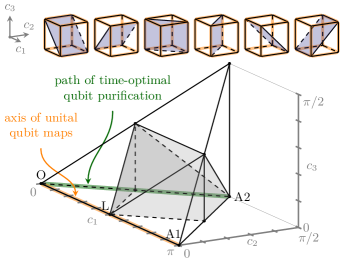
Figure 1: (Color online) Symmetries (upper part) and construction of the Weyl chamber (lower part) for the characterization of the non-local content of any two-qubit operation $\mathsf{U}\in\mathrm{SU}(4)$, cf. Eq. (1). The shaded polyhedron within the Weyl chamber describes all perfectly entangling operations. The orange line highlights those $\mathsf{U}$ which lead to unital maps for the qubit. The green line anticipates a time-optimal path for qubit purification identified below. The letters mark specific elements of $\mathrm{SU}(4)$ referred to in the text.

With this observation, we can relate non-unitality of $\mathcal{D}_{\mathsf{\rho}_{\mathrm{B}}(0)}$ with the entangling capability of $\mathsf{U}$ for the qubit-ancilla system. The latter is best analyzed in the Weyl chamber Zhang et al. (2003) which is a symmetry-reduced version of the cube spanned by $c_{1},c_{2},c_{3}\in[0,\pi]$, obtained when eliminating redundancies in Eq. (1). The six symmetries are sketched in the upper part of Fig. 1 with the Weyl chamber shown below. The shaded polyhedron in its center describes all perfectly entangling operations, and the $c_{1}$-axis represents all operations with at most one non-vanishing NL coordinate. It contains one point of the polyhedron of perfect entanglers—the point L corresponding to the gate cNOT and all gates that are locally equivalent to it, including cPHASE. Albeit being perfect entanglers, cNOT and cPHASE yield unital maps for the qubit. The capability of $\mathsf{U}$ to create entanglement between qubit and ancilla is thus a necessary but not a sufficient condition for purification of the qubit.

Next, we determine the qubit-ancilla couplings that allow for purification of the qubit. To this end, we write the qubit-ancilla Hamiltonian,

$$\mathsf{H}(t) =\mathsf{H}_{\mathrm{S}}(t)\otimes\mathsf{\mathbbm{1}}_{\mathrm{B}}+\mathsf{\mathbbm{1}}_{\mathrm{S}}\otimes\mathsf{H}_{\mathrm{B}}+\mathsf{H}_{\mathrm{int}}$$ (6)

with $\mathsf{H}_{\mathrm{S}}(t)=\frac{\omega_{\mathrm{S}}}{2}\mathsf{\sigma}_{3}+\mathcal{E}(t)\mathsf{O}_{\mathrm{c}}$, $\mathsf{H}_{\mathrm{B}}=\frac{\omega_{\mathrm{B}}}{2}\mathsf{\sigma}_{3}$, and $\mathsf{H}_{\mathrm{int}}=J\left(\mathsf{O}_{\mathrm{S}}\otimes\mathsf{O}_{\mathrm{B}}\right)$, assuming control, via an external field $\mathcal{E}(t)$, only over the qubit. $J$ denotes the qubit-ancilla coupling strength , $\omega_{\mathrm{S}}<\omega_{\mathrm{B}}$ are the level splittings of qubit and ancilla, and $\mathsf{O}_{\mathrm{S}},\mathsf{O}_{\mathrm{B}},\mathsf{O}_{\mathrm{c}}\in\{\mathsf{\sigma}_{1},\mathsf{\sigma}_{2},\mathsf{\sigma}_{3}\}$. To relate the Hamiltonian (6) to the purification condition, which is stated in terms of the number $N_{\mathrm{c}}$ of non-zero NL coordinates of the joint qubit-ancilla time evolution, we consider the dynamical Lie algebra $\mathcal{L}$. Its Cartan decomposition, $\mathcal{L}=\mathfrak{k}\oplus\mathfrak{p}$, implies that $\mathsf{A}$ in Eq. (1) is an element of the group $\exp\{\mathfrak{a}\}$ where $\mathfrak{a}$ is the Cartan subalgebra, i.e., the maximal Abelian subalgebra of $\mathfrak{p}$. For Hamiltonian (6) and the control task of purifying the qubit, it turns out that $N_{\mathrm{c}}=\mathrm{dim}\{\mathfrak{a}\}$ . Since $\mathfrak{a}$ can be determined entirely from the Hamiltonian, without any knowledge of the actual dynamics, $N_{\mathrm{c}}$ is readily obtained. It is thus straightforward to identify the combinations $\mathsf{O}_{\mathrm{S}},\mathsf{O}_{\mathrm{B}},\mathsf{O}_{\mathrm{c}}\in\{\mathsf{\sigma}_{1},\mathsf{\sigma}_{2},\mathsf{\sigma}_{3}\}$ for which $N_{\mathrm{c}}\geq 2$: Out of the $3\times 3\times 3$ possible combinations of $\mathsf{O}_{\mathrm{S}},\mathsf{O}_{\mathrm{B}},\mathsf{O}_{\mathrm{c}}$, only 16 have a Cartan subalgebra $\mathfrak{a}$ of dimension 2, allowing for purification of the qubit . Table SI in the supplemental material (SM) sup summarizes the resulting dynamical Lie algebras and presents possible choices for $\mathfrak{a}$.

After identifying the cases, in which Hamiltonian (6) allows for purification of the qubit, we seek to derive the fields $\mathcal{E}(t)$ which reset the qubit in minimum time. This requires consideration not only of the generators, but also of the full dynamics We assume a separable initial state with the ancilla in thermal equilibrium, i.e., without ancilla coherence,

$$\mathsf{\rho}(0)=\begin{pmatrix}p_{\mathrm{S}}^{\mathrm{e}}&\gamma_{\mathrm{S}}\\ \gamma_{\mathrm{S}}^{*}&p_{\mathrm{S}}^{\mathrm{g}}\end{pmatrix}\otimes\begin{pmatrix}p_{\mathrm{B}}^{\mathrm{e}}&0\\ 0&p_{\mathrm{B}}^{\mathrm{g}}\end{pmatrix}\,.$$ (7)

Before stating the general result, we present three observations based on numerical simulations of all 16 cases. (i) For a constant resonant field, the minimum time, $T_{\mathrm{min}}$, to achieve maximal qubit purity is independent of the initial qubit state, $\mathsf{\rho}_{\mathrm{S}}(0)$. Such a field puts qubit and ancilla into resonance, i.e., $\mathcal{E}$ is chosen such that $\lambda_{1}-\lambda_{0}=\omega_{\mathrm{B}}$ where $\lambda_{0}<\lambda_{1}$ are the field-dressed eigenvalues of the qubit Hamiltonian $\mathsf{H}_{\mathrm{S}}$. This generalizes the results of Ref. Basilewitsch et al. (2017) to the remaining 15 cases where purification is possible. (ii) The specific value of $T_{\mathrm{min}}$ depends on the type of qubit-ancilla interaction and local control, i.e., on the choice of $\mathsf{O}_{\mathrm{S}}$, $\mathsf{O}_{\mathrm{B}}$, $\mathsf{O}_{\mathrm{c}}$. (iii) When allowing for fully time-dependent control fields $\mathcal{E}(t)$, the maximal qubit purity cannot be reached faster than $T_{\mathrm{min}}$. For times $\tau<T_{\mathrm{min}}$, numerical optimizations using Krotov’s method Konnov and Krotov (1999); Reich et al. (2012) lead to an upper bound for the qubit purity $\mathcal{P}_{\mathrm{S}}(\tau)$, given in terms of the evolution of the thermal initial state $\mathsf{\rho}_{\mathrm{S}}(0)$. The optimally shaped fields saturating the bound depend both on the initial state and the choice of $\mathsf{O}_{\mathrm{S}}$, $\mathsf{O}_{\mathrm{B}}$, $\mathsf{O}_{\mathrm{c}}$.

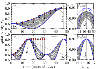
Figure 2: (Color online) The time evolution of the qubit purity reveals the minimum time for qubit reset – shown here for the examples $\mathsf{H}_{\mathrm{int}}=J(\mathsf{\sigma}_{1}\otimes\mathsf{\sigma}_{1})$ with $\mathsf{H}_{\mathrm{c}}(t)=\mathcal{E}(t)\,\mathsf{\sigma}_{1}$ (a) and $\mathsf{H}_{\mathrm{c}}(t)=\mathcal{E}(t)\,\mathsf{\sigma}_{3}$ (b). The gray area corresponds to the superimposed evolutions of fifty different initial states $\mathsf{\rho}(0)=\mathsf{\rho}_{\mathrm{S}}(0)\otimes\mathsf{\rho}_{\mathrm{B}}(0)$ with $\mathsf{\rho}_{\mathrm{B}}(0)$ the thermal equilibrium state and $\mathsf{\rho}_{\mathrm{S}}(0)$ sampled randomly under the condition of identical purity. The red (black) dots indicate the values for $\mathcal{P}_{\mathrm{S}}(\tau)$ obtained with optimized (constant resonant) $\mathcal{E}(t)$. The dashed blue lines indicate the upper and lower bounds of $\mathcal{P}_{\mathrm{S}}$ predicted by Eq. (8). $\mathcal{P}_{\mathrm{B}}(0)$ denotes the initial ancilla purity. The parameters are $\omega_{\mathrm{S}}=1$, $\omega_{\mathrm{B}}=3$, $J=0.1$, and inverse temperature $\beta=1$.

We discuss these observations in more detail for $\mathsf{O}_{\mathrm{S}}=\mathsf{O}_{\mathrm{B}}=\mathsf{\sigma}_{1}$ with (a) $\mathsf{O}_{\mathrm{c}}=\mathsf{\sigma}_{1}$ and (b) $\mathsf{O}_{\mathrm{c}}=\mathsf{\sigma}_{3}$, cf. Fig. 2. These two examples are paradigmatic, with all other combinations of $\mathsf{O}_{\mathrm{S}}$, $\mathsf{O}_{\mathrm{B}}$, and $\mathsf{O}_{\mathrm{c}}$ yielding identical results (data not shown). In case (b), we know that time-optimal reset is achieved with a constant field $\mathcal{E}(t)=\mathcal{E}$ that puts qubit and ancilla into resonance Basilewitsch et al. (2017). A constant resonant field therefore seems to be a suitable pilot for all numerical optimizations. For all initial states of the qubit (randomly chosen under the condition of identical purity), a maximum in the time evolution of the purity occurs at roughly the same point in time, $T_{\mathrm{min}}$, when applying the constant resonant field, cf. Fig. 2. Using optimal control theory, we find field shapes $\mathcal{E}(t)$, $t\in[0,\tau]$, that maximize $\mathcal{P}_{\mathrm{S}}(\tau)$ at a given time $\tau$. For a few choices of $\tau$, the black and red dots in Fig. 2 compare the purities obtained with constant resonant and optimized fields . In all cases with $\tau\neq T_{\mathrm{min}}$, the optimized fields improve the purity compared to the constant resonant field. For $\tau=T_{\mathrm{min}}$, the purities coincide (since the constant resonant field is already an optimal solution). For $\tau<T_{\mathrm{min}}$, there exists an upper bound for $\mathcal{P}_{\mathrm{S}}(\tau)$, which is attained by the constant resonant field for a coherence-free initial qubit state with $p_{\mathrm{S}}^{\mathrm{g}}>p_{\mathrm{S}}^{\mathrm{e}}$. This bound can be proven rigorously Ticozzi and Viola (2014); sup . While the individual optimized fields depend on $\tau$ and, for $\tau\neq T_{\mathrm{min}}$, on the initial state of the qubit, they all exhibit a strong off-resonant initial peak which, if $\gamma_{S}\neq 0$, rotates the coherence into population or, if $p_{\mathrm{S}}^{\mathrm{g}}<p_{\mathrm{S}}^{\mathrm{e}}$, inverts the qubit populations, before swapping the purities with the resonant protocol Basilewitsch et al. (2017). When allowing for times $\tau>T_{\mathrm{min}}$, a purity swap between qubit and ancilla remains the optimal strategy, with the corresponding fields being more complex than the constant resonant solution for $\tau=T_{\mathrm{min}}$.

Based on these numerical results, we conjecture that time-optimal purification requires one to choose a constant and resonant field, $\mathcal{E}(t)=\mathcal{E}$ such that $\lambda_{1}-\lambda_{0}=\omega_{\mathrm{B}}$, independent of $\mathsf{O}_{\mathrm{S}}$, $\mathsf{O}_{\mathrm{B}}$ and $\mathsf{O}_{\mathrm{c}}$. For this choice of $\mathcal{E}(t)$, an exact closed-form expression for the joint time evolution operator can be approximated to yield an expression for the time evolution of the qubit purity, cf. SM sup . For the example of case (a), it reads

$$\mathcal{P}_{\mathrm{S}}(t) \approx \Big{[}p_{\mathrm{S}}^{\mathrm{g}}p_{\mathrm{B}}^{\mathrm{g}}+p_{\mathrm{S}}^{\mathrm{g}}p_{\mathrm{B}}^{\mathrm{e}}\cos^{2}(\eta t)+p_{\mathrm{S}}^{\mathrm{e}}p_{\mathrm{B}}^{\mathrm{g}}\sin^{2}(\eta t)\Big{]}^{2}$$ (8)

$$+\Big{[}p_{\mathrm{S}}^{\mathrm{e}}p_{\mathrm{B}}^{\mathrm{e}}+p_{\mathrm{S}}^{\mathrm{g}}p_{\mathrm{B}}^{\mathrm{e}}\sin^{2}(\eta t)+p_{\mathrm{S}}^{\mathrm{e}}p_{\mathrm{B}}^{\mathrm{g}}\cos^{2}(\eta t)\Big{]}^{2}$$

$$+2|\gamma_{\mathrm{S}}|^{2}\cos^{2}(\eta t)$$

with

$$\eta^{2}=J^{2}+\frac{\omega_{\mathrm{B}}}{2}\left(\omega_{\mathrm{B}}-\sqrt{\omega_{\mathrm{B}}^{2}+4B^{2}}\right),\;B^{2}=J^{2}\frac{\omega_{\mathrm{B}}^{2}-\omega_{\mathrm{S}}^{2}}{\omega_{\mathrm{B}}^{2}}.$$ (9)

Maximizing $\mathcal{P}_{\mathrm{S}}(t)$ yields an approximated minimum time for purification, $T_{\mathrm{min}}=\pi/(2\eta)$, independent of the initial state. This explains why $\mathcal{P}_{\mathrm{S}}(t)$ displays a perfect swap of qubit and ancilla purity at $T_{\mathrm{min}}$ for all evolutions in Fig. 2(a). For all other Hamiltonians which allow for purification, we obtain the same result for $\mathcal{P}_{\mathrm{S}}(t)$, Eq. (8), but with different expressions for $\eta$ and $B$ sup . For example, in case (b) $B=0$ and hence $\eta=J$ leads to $T_{\mathrm{min}}=\pi/(2J)$, which is much shorter than $T_{\mathrm{min}}$ in case (a) where $B\neq 0$, cf. Fig. 2.

Overall, we find three distinct minimal reset times which can be linked to a single quantity $A$ with $T_{\mathrm{min}}\approx\pi/(2|A|)$. The parameter $A$ can be obtained analytically from the Hamiltonian and is determined by the parameters $J$, $\omega_{\mathrm{S}}$ and $\omega_{\mathrm{B}}$ for all possible combinations of $\mathsf{O}_{\mathrm{S}},\mathsf{O}_{\mathrm{B}},\mathsf{O}_{\mathrm{c}}\in\{\mathsf{\sigma}_{1},\mathsf{\sigma}_{2},\mathsf{\sigma}_{3}\}$, cf. SM sup . The minimal times depending on the choice of $\mathsf{O}_{\mathrm{S}},\mathsf{O}_{\mathrm{B}},\mathsf{O}_{\mathrm{c}}$ are sup : $T^{(1)}_{\mathrm{min}}=\pi/(2J)$, $T^{(2)}_{\mathrm{min}}=\pi/(2J)\cdot\omega_{\mathrm{B}}/\omega_{\mathrm{S}}$, and $T^{(3)}_{\mathrm{min}}=\pi/(2J)\cdot\omega_{\mathrm{B}}/\sqrt{\omega_{\mathrm{B}}^{2}-\omega_{\mathrm{S}}^{2}}$, see also Table 1. Among these, $T^{(1)}_{\mathrm{min}}$ represents the global minimum, as we prove rigorously in the SM sup , using the Time-optimal tori theorem for $\mathrm{SU}(4)$ Khaneja et al. (2001). Remarkably, we find that, for qubit reset, the global minimum $T^{(1)}_{\mathrm{min}}$ can be attained with a single control field acting on the qubit only, whereas the Time-optimal tori theorem assumes full controllability over system and ancilla. When allowing $\mathsf{O}_{\mathrm{S}}$, $\mathsf{O}_{\mathrm{B}}$ and $\mathsf{O}_{\mathrm{c}}$ to be arbitrary elements of $\mathfrak{su}(2)=\mathrm{span}\{\mathsf{\sigma}_{1},\mathsf{\sigma}_{2},\mathsf{\sigma}_{3}\}$ including superpositions of Pauli operators, we find the respective minimum times for the purity swap to be lower bounded by $T^{(1)}_{\mathrm{min}}$, cf. SM sup .

Table 1: Minimum reset times $T_{\mathrm{min}}$ for two coupled superconducting qubits Rigetti et al. (2005) with three sets of experimental parameters (set 1: $\omega_{\mathrm{S}}/(2\pi)=12.8$ GHz, $\omega_{\mathrm{B}}/(2\pi)=16.1$ GHz, $J/(2\pi)=65$ MHz; set 2: $\omega_{\mathrm{S}}/(2\pi)=9.8$ GHz, $\omega_{\mathrm{B}}/(2\pi)=16.1$ GHz, $J/(2\pi)=200$ MHz; set 3: $\omega_{\mathrm{S}}/(2\pi)=15.8$ GHz, $\omega_{\mathrm{B}}/(2\pi)=16.1$ GHz, $J/(2\pi)=25$ MHz Rigetti and Devoret (2010)).

$\mathsf{O}_{\mathrm{S}}\otimes\mathsf{O}_{\mathrm{B}}$	$\mathsf{O}_{\mathrm{c}}$	$T_{\mathrm{min}}$ (set 1)	$T_{\mathrm{min}}$ (set 2)	$T_{\mathrm{min}}$ (set 3)
$\mathsf{\sigma}_{1}\otimes\mathsf{\sigma}_{1}$	$\mathsf{\sigma}_{1}$	$191.0$ ns	$81.1$ ns	$402.3$ ns
$\mathsf{\sigma}_{1}\otimes\mathsf{\sigma}_{1}$	$\mathsf{\sigma}_{2}$	$151.8$ ns	$49.3$ ns	$394.8$ ns
$\mathsf{\sigma}_{1}\otimes\mathsf{\sigma}_{1}$	$\mathsf{\sigma}_{3}$	$151.8$ ns	$49.3$ ns	$394.8$ ns
$\mathsf{\sigma}_{1}\otimes\mathsf{\sigma}_{2}$	$\mathsf{\sigma}_{1}$	$191.0$ ns	$81.1$ ns	$402.3$ ns
$\mathsf{\sigma}_{1}\otimes\mathsf{\sigma}_{2}$	$\mathsf{\sigma}_{2}$	$151.8$ ns	$49.3$ ns	$394.8$ ns
$\mathsf{\sigma}_{1}\otimes\mathsf{\sigma}_{2}$	$\mathsf{\sigma}_{3}$	$151.8$ ns	$49.3$ ns	$394.8$ ns
$\mathsf{\sigma}_{2}\otimes\mathsf{\sigma}_{1}$	$\mathsf{\sigma}_{1}$	$151.8$ ns	$49.3$ ns	$394.8$ ns
$\mathsf{\sigma}_{2}\otimes\mathsf{\sigma}_{1}$	$\mathsf{\sigma}_{2}$	$191.0$ ns	$81.1$ ns	$402.3$ ns
$\mathsf{\sigma}_{2}\otimes\mathsf{\sigma}_{1}$	$\mathsf{\sigma}_{3}$	$151.8$ ns	$49.3$ ns	$394.8$ ns
$\mathsf{\sigma}_{2}\otimes\mathsf{\sigma}_{2}$	$\mathsf{\sigma}_{1}$	$151.8$ ns	$49.3$ ns	$394.8$ ns
$\mathsf{\sigma}_{2}\otimes\mathsf{\sigma}_{2}$	$\mathsf{\sigma}_{2}$	$191.0$ ns	$81.1$ ns	$402.3$ ns
$\mathsf{\sigma}_{2}\otimes\mathsf{\sigma}_{2}$	$\mathsf{\sigma}_{3}$	$151.8$ ns	$49.3$ ns	$394.8$ ns
$\mathsf{\sigma}_{3}\otimes\mathsf{\sigma}_{1}$	$\mathsf{\sigma}_{1}$	$250.3$ ns	$62.2$ ns	$2054.6$ ns
$\mathsf{\sigma}_{3}\otimes\mathsf{\sigma}_{1}$	$\mathsf{\sigma}_{2}$	$250.3$ ns	$62.2$ ns	$2054.6$ ns
$\mathsf{\sigma}_{3}\otimes\mathsf{\sigma}_{2}$	$\mathsf{\sigma}_{1}$	$250.3$ ns	$62.2$ ns	$2054.6$ ns
$\mathsf{\sigma}_{3}\otimes\mathsf{\sigma}_{2}$	$\mathsf{\sigma}_{2}$	$250.3$ ns	$62.2$ ns	$2054.6$ ns

Table 1 shows exemplary minimum reset times $T_{\mathrm{min}}$ for a physical realization of two coupled superconducting qubits Rigetti et al. (2005); Rigetti and Devoret (2010), illustrating the role of device design in terms of the choice of $\mathsf{O}_{\mathrm{S}}$, $\mathsf{O}_{\mathrm{B}}$, and $\mathsf{O}_{\mathrm{c}}$ as well as the parameters $\omega_{\mathrm{S}},\ \omega_{\mathrm{B}}$ and $J$. In case of the optimal choice of $\mathsf{O}_{\mathrm{S}}$, $\mathsf{O}_{\mathrm{B}}$, and $\mathsf{O}_{\mathrm{c}}$ such that $T_{\mathrm{min}}=T^{(1)}_{\mathrm{min}}$ (independently of $\omega_{B}$), $\omega_{B}$ should be chosen as large as possible to increase the maximum achievable purity. An option to effectively enlarge $\omega_{B}$ is to utilize ancilla levels above the two-level subspace. This raises the question whether our findings on minimum protocol duration and maximum reset fidelity hold also for ancillas with Hilbert space dimension larger than two.

Numerical simulations for a three-level and four-level ancilla suggest that the reset time for ancillas with Hilbert space dimension larger than two is still lower bounded by $T^{(1)}_{\mathrm{min}}=\pi/(2J)$ sup . In contrast, the maximally reachable qubit purity increases and can be brought close to one for ancillas with Hilbert space dimension $d_{\mathrm{B}}\geq 4$, provided half of the eigenvalues of the initial ancilla state are small sup . If we consider, for example, an ancilla with equidistant energy levels ($\omega_{\mathrm{B}}=3$) and thermal initial states on qubit ($\omega_{\mathrm{S}}=1$) and ancilla with $\beta=1$, the maximal achievable purity increases from $\mathcal{P}\approx 0.970$ for $d_{\mathrm{B}}=3$ to $\mathcal{P}\approx 0.995$ for $d_{\mathrm{B}}=4$, while $\mathcal{P}\approx 0.905$ for a two-level ancilla. These conditions can easily be realized by utilizing higher excited levels of transmon qubits or superconducting resonators. Such ancillas would also provide for complete controllability Geerlings et al. (2013); Magnard et al. (2018); Egger et al. (2018) which may be required to realize the spectral reshuffling of the joint initial state that implements an optimal reset dynamics, as we discuss in more detail in the SM sup .

To conclude, we have shown that there exists a globally minimal time (among all Hamiltonians) to reset a qubit with maximal fidelity when making use of an ancilla and time-dependent external control fields over the qubit. For two-level ancillas, a time-optimal protocol ensures resonance between qubit and ancilla and swaps their purities. The reset fidelity is then determined by the initial ancilla purity, making it crucial to engineer a sufficiently high ancilla purity, or, respectively, low ancilla temperature. Due to its non-trivial dependence on the effective qubit-ancilla coupling strength, there exists an optimal choice for qubit-ancilla interaction and type of local control for the time-optimal reset. Thanks to the Cartan decomposition of SU(4), this choice can be determined at the level of the algebra, i.e., the Hamiltonian, and does not require knowledge of the actual reset dynamics. For ancillas with Hilbert space dimension larger than three, the qubit purity can be brought arbitrarily close to one by proper spectral reshuffling of the joint qubit ancilla state, provided at least half of the ancilla levels have negligible population. The corresponding experimental conditions on ancilla state and control are easily met by e.g. current superconducting qubit technology. Our results provide the guiding principles for device design in order to realize the fastest and most accurate protocol for qubit reset in a given QI architecture.