Generalized Prager-Synge Inequality and
Equilibrated Error Estimators for Discontinuous Elements

Abstract

The well-known Prager-Synge identity is valid in $H^{1}(\Omega)$ and serves as a foundation for developing equilibrated a posteriori error estimators for continuous elements. In this paper, we introduce a new inequality, that may be regarded as a generalization of the Prager-Synge identity, to be valid for piecewise $H^{1}(\Omega)$ functions for diffusion problems. The inequality is proved to be identity in two dimensions.

For nonconforming finite element approximation of arbitrary odd order, we propose a fully explicit approach that recovers an equilibrated flux in $H({\rm div};\Omega)$ through a local element-wise scheme and that recovers a gradient in $H({\rm curl};\Omega)$ through a simple averaging technique over edges. The resulting error estimator is then proved to be globally reliable and locally efficient. Moreover, the reliability and efficiency constants are independent of the jump of the diffusion coefficient regardless of its distribution.

1 Introduction

Equilibrated a posteriori error estimators have attracted much interest recently due to the guaranteed reliability bound with the reliability constant being one. This property implies that they are perfect for discretization error control on both coarse and fine meshes. Error control on coarse meshes is important but difficult for computationally challenging problems.

For the conforming finite element approximation, a mathematical foundation of equilibrated estimators is the Prager-Synge identity [31] that is valid in $H^{1}(\Omega)$ (see Section 3). Based on this identity, various equilibrated estimators have been studied recently by many researchers (see, e.g., [27, 22, 29, 20, 21, 6, 3, 33, 10, 12, 13, 34, 17, 14]). The key ingredient of the equilibrated estimators for the continuous elements is local recovery of an equilibrated (locally conservative) flux in the $H({\rm div};\Omega)$ space through the numerical flux. By using a partition of unity, Ladevèze and Leguillon [27] initiated a local procedure to reduce the construction of an equilibrated flux to vertex patch based local calculations. For the continuous linear finite element approximation to the Poisson equation in two dimensions, an equilibrated flux in the lowest order Raviart-Thomas space was explicitly constructed in [10, 12]. This explicit approach does not lead to robust equilibrated estimator with respect to the coefficient jump without introducing a constraint minimization (see [17]). The constraint minimization on each vertex patch may be efficiently solved by first computing an equilibrated flux and then calculating a divergence free correction. For recent developments, see [14] and references therein.

The purpose of this paper is to develop and analyze equilibrated a posteriori error estimators for discontinuous elements including both nonconforming and discontinuous Galerkin elements. To do so, the first and the essential step is to extend the Prager-Synge identity to be valid for piecewise $H^{1}(\Omega)$ functions. This will be done by establishing a generalized Prager-Synge inequality (see Theorem 3.1) that contains an additional term measuring the distance between $H^{1}(\Omega)$ and piecewise $H^{1}(\Omega)$. Moreover, by using a Helmholtz decomposition, we will be able to show that the inequality becomes an identity in two dimensions (see Lemma 3.4). A non-optimal inequality similar to ours was obtained earlier by Braess, Fraunholz, and Hoppe in [11] for the Poisson equation with pure Dirichlet boundary condition. Based on the generalized Prager-Synge inequality and an equivalent form (see Corollary 3.2), the construction of an equilibrated a posteriori error estimator for discontinuous finite element solutions is reduced to recover an equilibrated flux in $H(\mbox{div};\Omega)$ and to recover either a potential function in $H^{1}(\Omega)$ or a curl free vector-valued function in $H({\rm curl};\Omega)$.

Recovery of equilibrated fluxes for discontinuous elements has been studied by many researchers. For discontinuous Garlerkin (DG) methods, equilibrated fluxes in Raviart-Thomas (RT) spaces were explicitly reconstructed in [2] for linear elements and in [23] for higher order elements. For nonconforming finite element methods, existing explicit equilibrated flux recoveries in RT spaces seem to be limited to the linear Crouzeix-Raviart (CR) and the quadratic Fortin-Soulie elements by Marini [28] (see [1] in the context of estimator) and Kim [26], respectively. For higher order nonconforming elements, a local reconstruction procedure was proposed by Ainsworth and Rankin in [4] through solving element-wise minimization problems. The recovered flux is not in the RT spaces. Nevertheless, the resulting estimator provides a guaranteed upper bound.

In this paper, we will introduce a fully explicit post-processing procedure for recovering an equilibrated flux in the RT space of index $k-1$ for the nonconforming elements of odd order of $k\geq 1$. Currently, we are not able to extend our recovery technique to even orders. This is because our recovery procedure heavily depends on the finite element formulation and the properties of the nonconforming finite element space; moreover, structure of the nonconforming finite element spaces of even and odd orders are fundamentally different.

Recovery of a potential function in $H^{1}(\Omega)$ for discontinuous elements was studied by some researchers (see, e.g., [4, 2, 11]). Local approaches for recovering equilibrated flux in [10, 12, 17, 13, 14] may be directly applied (at least in two dimensions) for computing an approximation to the gradient in the curl-free space. (As mentioned previously, this approach requires solutions of local constraint minimization problems over vertex patches.) The resulting a posteriori error estimator from either the potential or the gradient recoveries may be proved to be locally efficient. Nevertheless, to show independence of the efficiency constant on the jump, we have to assume that the distribution of the diffusion coefficient is quasi-monotone (see [30]).

In this paper, we will employ a simple averaging technique over edges to recover a gradient in $H({\rm curl};\Omega)$. Due to the fact that the recovered gradient is not necessarily curl free, the reliability constant of the resulting estimator is no longer one. However, it turns out that the curl free constraint is not essential and, theoretically we are able to prove that the resulting estimator has the robust local reliability as well as the robust local efficiency without the quad-monotone assumption. This is compatible with our recent result in [15] on the residual error estimator for discontinuous elements.

This paper is organized as follows. The diffusion problem and the finite element mesh are introduced in Section 2. The generalized Prager-Synge inequality for piecewise $H^{1}(\Omega)$ functions are established in Section 3. Explicit recoveries of an equilibrated flux and a gradient and the resulting a posteriori error estimator for discontinuous elements are described in Section 4. Global reliability and local efficiency of the estimator are proved in Section 5. Finally, numerical results are presented in Section 6.

2 Model problem

Let $\Omega$ be a bounded polygonal domain in $\mathbb{R}^{d},d=2,3$, with Lipschitz boundary $\partial\Omega=\overline{\Gamma}_{D}\cup\overline{\Gamma}_{N}$, where $\overline{\Gamma}_{D}\cap\overline{\Gamma}_{N}=\emptyset$. For simplicity, assume that $\mbox{meas}_{d-1}(\Gamma_{D})\neq 0$. Considering the diffusion problem:

$$-\nabla\cdot(A\nabla u)=f\quad\mbox{in}\quad\Omega,$$ (2.1)

with boundary conditions

$$u=0\;\mbox{ on }\Gamma_{D}\quad\mbox{and}\quad-A\nabla u\cdot{\bf n}=g\;\mbox{ on }\Gamma_{N},$$

where $\nabla\cdot$ and $\nabla$ are the respective divergence and gradient operators; ${\bf n}$ is the outward unit vector normal to the boundary; $f\in L^{2}(\Omega)$ and $g\in H^{-1/2}(\Gamma_{N})$ are given scalar-valued functions; and the diffusion coefficient $A(x)$ is symmetric, positive definite, and piecewise constant full tensor with respect to the domain $\overline{\Omega}=\cup_{i=1}^{n}\overline{\Omega}_{i}$. Here we assume that the subdomain, $\Omega_{i}$ for $i=1,\cdots,n$, is open and polygonal.

We use the standard notations and definitions for the Sobolev spaces. Let

$$H_{D}^{1}(\Omega)=\left\{v\in H^{1}(\Omega)\,:\,v=0\mbox{ on }\Gamma_{D}\right\}.$$

Then the corresponding variational problem of (2.1) is to find $u\in H^{1}_{D}(\Omega)$ such that

$$a(u,\,v):=(A\nabla u,\nabla v)=(f,v)-\left<g,v\right>_{\Gamma_{N}},\quad\forall\;v\in H_{D}^{1}(\Omega),$$ (2.2)

where $(\cdot,\cdot)_{\omega}$ is the $L^{2}$ inner product on the domain $\omega$. The subscript $\omega$ is omitted when $\omega=\Omega$.

2.1 Triangulation

Let ${\cal T}=\{K\}$ be a finite element partition of $\Omega$ that is regular, and denote by $h_{K}$ the diameter of the element $K$. Furthermore, assume that the interfaces,

$$\Gamma=\{\partial\Omega_{i}\cap\partial\Omega_{j}:i\neq j\mbox{ and }i,j=1,\cdots,n\},$$

do not cut through any element $K\in{\cal T}$. Denote the set of all edges of the triangulation ${\cal T}$ by

$${\cal E}:={\cal E}_{I}\cup{\cal E}_{D}\cup{\cal E}_{N},$$

where ${\cal E}_{I}$ is the set of interior element edges, and ${\cal E}_{D}$ and ${\cal E}_{N}$ are the sets of boundary edges belonging to the respective $\Gamma_{D}$ and $\Gamma_{N}$. For each $F\in{\cal E}$, denote by $h_{F}$ the length of $F$ and by ${\bf n}_{F}$ a unit vector normal to $F$. Let $K_{F}^{+}$ and $K_{F}^{-}$ be the two elements sharing the common edge $F\in{\cal E}_{I}$ such that the unit outward normal of $K_{F}^{-}$ coincides with ${\bf n}_{F}$. When $F\in{\cal E}_{D}\cup{\cal E}_{N}$, ${\bf n}_{F}$ is the unit outward normal to $\partial\Omega$ and denote by $K_{F}^{-}$ the element having the edge $F$.

3 Generalized Prager-Synge inequality

For the conforming finite element approximation, the foundation of the equilibrated a posteriori error estimator is the Prager-Synge identity [31]. That is, let $u\in H^{1}_{D}(\Omega)$ be the solution of (2.1), then

$$\|A^{1/2}\nabla\,(u-w)\|^{2}+\|A^{-1/2}\mbox{\boldmath$\tau$}+A^{1/2}\nabla\,u\|^{2}=\|A^{-1/2}\mbox{\boldmath$\tau$}+A^{1/2}\nabla\,w\|^{2}$$

for all $w\in H^{1}_{D}(\Omega)$ and for all $\mbox{\boldmath$\tau$}\in\Sigma_{f}(\Omega)$, where $\Sigma_{f}(\Omega)$ is the so-called equilibrated flux space defined by

$$\Sigma_{f}(\Omega)=\Big{\{}\mbox{\boldmath$\tau$}\in H({\rm div};\Omega):\nabla\cdot\mbox{\boldmath$\tau$}=f\mbox{ in }\Omega\;\mbox{ and }\;\mbox{\boldmath$\tau$}\cdot{\bf n}=g_{{}_{N}}\Big{\}}.$$

Here, $H({\rm div};\Omega)\subset L^{2}(\Omega)^{d}$ denotes the space of all vector-valued functions whose divergence are in $L^{2}(\Omega)$. The Prager-Synge identity immediately leads to

$$\|A^{1/2}\nabla\,(u-w)\|^{2}\leq\inf_{\mbox{\boldmath$\tau$}\in\Sigma_{f}(\Omega)}\|A^{-1/2}\mbox{\boldmath$\tau$}+A^{1/2}\nabla\,w\|^{2}.$$ (3.1)

Choosing $w\in H^{1}_{D}(\Omega)$ to be the conforming finite element approximation, then (3.1) implies that

$$\eta_{\tau}:=\|A^{-1/2}\mbox{\boldmath$\tau$}+A^{1/2}\nabla\,w\|,\quad\forall\,\,\mbox{\boldmath$\tau$}\in\Sigma_{f}(\Omega)$$ (3.2)

is a reliable estimator with the reliability constant being one.

We now proceed to establish a generalization of (3.1) for piecewise $H^{1}(\Omega)$ functions with applications to nonconforming and discontinuous Galerkin finite element approximations. To this end, denote the broken $H^{1}(\Omega)$ space with respect to ${\cal T}$ by

$$H^{1}({\cal T})=\left\{v\in L^{2}(\Omega)\,:\,v|_{K}\in H^{1}(K),\quad\forall\,K\in{\cal T}\right\}.$$

Define $\nabla_{h}$ be the discrete gradient operator on $H^{1}({\cal T})$ such that for any $v\in H^{1}({\cal T})$

$$(\nabla_{h}v)|_{K}=\nabla(v|_{K}),\quad\forall K\in{\cal T}.$$

Theorem 3.1.

Let $u\in H^{1}_{D}(\Omega)$ be the solution of (2.1). In both two and three dimensions, for all $w\in H^{1}({\cal T})$, we have

$$\|A^{1/2}\nabla_{h}(u-w)\|^{2}\leq\inf_{\mbox{\boldmath$\tau$}\in\Sigma_{f}(\Omega)}\|A^{-1/2}\mbox{\boldmath$\tau$}+A^{1/2}\nabla_{h}w\|^{2}+\inf_{v\in H^{1}_{D}(\Omega)}\|A^{1/2}\nabla_{h}(v-w)\|^{2}.$$ (3.3)

Proof.

Let $w\in H^{1}({\cal T})$, for all $\mbox{\boldmath$\tau$}\in\Sigma_{f}(\Omega)$ and for all $v\in H_{D}^{1}(\Omega)$, it follows from integration by parts and the Cauchy-Schwarz and Young’s inequalities that

$$2\,(\nabla_{h}(u-w),A\nabla u+\mbox{\boldmath$\tau$}) = 2\,(\nabla(u-v),A\nabla u+\mbox{\boldmath$\tau$})+2\,(\nabla_{h}(v-w),A\nabla u+\mbox{\boldmath$\tau$})$$ (3.4)

$$= 2\,(\nabla_{h}(v-w),A\nabla u+\mbox{\boldmath$\tau$})$$

$$\leq \|A^{1/2}\nabla_{h}(v-w)\|^{2}+\|A^{1/2}\nabla u+A^{-1/2}\mbox{\boldmath$\tau$}\|^{2}.$$

It is easy to see that

$$\|A^{1/2}\nabla_{h}w+A^{-1/2}\mbox{\boldmath$\tau$}\|^{2}=\|A^{1/2}\nabla_{h}(u-w)\|^{2}+\|A^{1/2}\nabla u+A^{-1/2}\mbox{\boldmath$\tau$}\|^{2}-2(\nabla_{h}(u-w),A\nabla u+\mbox{\boldmath$\tau$}),$$

which, together with (3.4), implies

$$\|A^{1/2}\nabla_{h}(u-w)\|^{2}$$

$$= \|A^{1/2}\nabla_{h}w+A^{-1/2}\mbox{\boldmath$\tau$}\|^{2}-\|A^{1/2}\nabla u+A^{-1/2}\mbox{\boldmath$\tau$}\|^{2}+2(\nabla_{h}(u-w),A\nabla u+\mbox{\boldmath$\tau$})$$

$$\leq \|A^{1/2}\nabla_{h}w+A^{-1/2}\mbox{\boldmath$\tau$}\|^{2}+\|A^{1/2}\nabla_{h}(v-w)\|^{2}$$

for all $\mbox{\boldmath$\tau$}\in\Sigma_{f}(\Omega)$ and all $v\in H_{D}^{1}(\Omega)$. This implies the validity of (3.3) and, hence, the theorem. ∎

A suboptimal result for the Poisson equation ($A=I$) with pure Dirichlet boundary condition is proved in [11] by Braess, Fraunholz, and Hoppe:

$$\|\nabla_{h}(u-w)\|\leq\inf_{\mbox{\boldmath$\tau$}\in\Sigma_{f}(\Omega)}\|\nabla w+\mbox{\boldmath$\tau$}\|+2\inf_{v\in H^{1}_{0}(\Omega)}\|\nabla_{h}(v-w)\|.$$

Let $H({\rm curl};\Omega)\subset L^{2}(\Omega)^{d}$ be the space of all vector-valued functions whose curl are in $L^{2}(\Omega)$, and denote its curl free subspace by

$$\mathring{H}_{D}({\rm curl};\Omega)=\left\{\mbox{\boldmath$\tau$}\in H({\rm curl};\Omega):{\nabla\times}\mbox{\boldmath$\tau$}=0\mbox{ in }\Omega\mbox{ and }\mbox{\boldmath$\tau$}\cdot{\bf t}=0\mbox{ on }\Gamma_{D}\right\},$$

where ${\bf t}$ denotes the tangent vector(s).

Corollary 3.2.

Let $u\in H^{1}_{D}(\Omega)$ be the solution of (2.1). In both two and three dimensions, for all $w\in H^{1}({\cal T})$, we have

$$\|A^{1/2}\nabla_{h}(u-w)\|^{2}\leq\inf_{\mbox{\boldmath$\tau$}\in\Sigma_{f}(\Omega)}\|A^{-1/2}\mbox{\boldmath$\tau$}+A^{1/2}\nabla_{h}w\|^{2}+\inf_{\mbox{\boldmath$\gamma$}\in\mathring{H}_{D}({\rm curl};\Omega)}\|A^{1/2}(\mbox{\boldmath$\gamma$}-\nabla_{h}w)\|^{2}.$$ (3.5)

Proof.

The result of (3.5) is an immediate consequence of (3.3) and the fact that $\nabla H^{1}_{D}(\Omega)=\mathring{H}_{D}({\rm curl};\Omega)$. ∎

In the remaining section, we prove that, in two dimensions, the inequality (3.3) in Theorem 3.1 is indeed an equality. For each $F\in{\cal E}$, in two dimensions, assume that ${\bf n}_{F}=(n_{{}_{1,F}},n_{{}_{2,F}})$, then denote by ${\bf t}_{F}=(-n_{{}_{2,F}},n_{{}_{1,F}})$ the unit vector tangent to $F$ and by ${\bf s}_{{}_{F}}$ and ${\bf e}_{{}_{F}}$ the start and end points of $F$, respectively, such that ${\bf e}_{{}_{F}}-{\bf s}_{{}_{F}}=h_{F}{\bf t}_{F}$. Let

$${\cal H}=\left\{v\in H^{1}(\Omega):\int_{\Omega}v\,dx=0\mbox{ and }\displaystyle\frac{\partial v}{\partial{\bf t}}=0\mbox{ on }\Gamma_{N}\right\}.$$

For a vector-valued function $\mbox{\boldmath$\tau$}=(\tau_{1},\tau_{2})\in H({\rm curl};\Omega)$, define the curl operator by

$${\nabla\times}\mbox{\boldmath$\tau$}=\displaystyle\frac{\partial\tau_{2}}{\partial x}-\displaystyle\frac{\partial\tau_{1}}{\partial y}.$$

For a scalar-valued function $v\in H^{1}(\Omega)$, define the formal adjoint operator of the curl by

$$\nabla^{\perp}v=\left(\displaystyle\frac{\partial v}{\partial y},\,-\displaystyle\frac{\partial v}{\partial x}\right).$$

For a fixed $w\in H^{1}({\cal T})$, there exist unique $\phi\in H_{D}^{1}(\Omega)$ and $\psi\in{\cal H}$ for the following Helmholtz decomposition (see, e.g., [4]) such that

$$A\nabla_{h}(u-w)=A\nabla\phi+\nabla^{\perp}\psi,$$ (3.6)

and $\phi$ and $\psi$ satisfy

$$(A\nabla\phi,\nabla v)=(A\nabla_{h}(u-w),\nabla v)\quad\forall v\in H_{D}^{1}(\Omega),$$

and

$$(A^{-1}\nabla^{\perp}\psi,\nabla^{\perp}w)=(\nabla_{h}(u-w),\nabla^{\perp}w)\quad\forall w\in{\cal H},$$

respectively. It is easy to see that $\nabla\phi$ and $\nabla^{\perp}\psi$ are orthogonal with respect to the $L^{2}$ inner product, which yields

$$\|A^{1/2}\nabla_{h}(u-w)\|^{2}=\|A^{1/2}\nabla\phi\|^{2}+\|A^{-1/2}\nabla^{\perp}\psi\|^{2}.$$ (3.7)

Lemma 3.3.

Let $w$ be a fixed function in $H^{1}({\cal T})$ and $\phi$ and $\psi$ be the corresponding Helmholtz decomposition of $w$ given in (3.6). We have

$$\inf_{\mbox{\boldmath$\tau$}\in\Sigma_{f}(\Omega)}\!\!\|A^{-1/2}\mbox{\boldmath$\tau$}+A^{1/2}\nabla_{h}w\|=\|A^{1/2}\nabla\phi\|\mbox{ and }\inf_{v\in H^{1}_{D}(\Omega)}\!\!\|A^{1/2}\nabla_{h}(v-w)\|=\|A^{-1/2}\nabla^{\perp}\psi\|.$$ (3.8)

Proof.

For any $\mbox{\boldmath$\tau$}\in\Sigma_{f}(\Omega)$, (3.6) and integration by parts give

$$\|A^{1/2}\nabla\phi\|^{2}=(A\nabla_{h}(u-w),\nabla\phi)=(A\nabla u+\mbox{\boldmath$\tau$},\nabla\phi)-(\mbox{\boldmath$\tau$}+A\nabla_{h}w,\nabla\phi)=-(\mbox{\boldmath$\tau$}+A\nabla_{h}w,\nabla\phi),$$

which, together with the Cauchy-Schwarz inequality and the choice $\mbox{\boldmath$\tau$}=\nabla^{\perp}\psi-A\nabla u\in\Sigma_{f}(\Omega)$, yields the first equality in (3.8) as follows:

$$\|A^{1/2}\nabla\phi\|\leq\inf_{\mbox{\boldmath$\tau$}\in\Sigma_{f}(\Omega)}\|A^{-1/2}\mbox{\boldmath$\tau$}+A^{1/2}\nabla_{h}w\|\leq\|A^{1/2}\nabla_{h}(u-w)-A^{-1/2}\nabla^{\perp}\psi\|=\|A^{1/2}\nabla\phi\|.$$

Now we proceed to prove the second equality in (3.8). For any $v\in H_{D}^{1}(\Omega)$, by (3.6) and integration by parts, we have

$$\|A^{-1/2}\nabla^{\perp}\psi\|^{2}=(\nabla_{h}(u-w),\nabla^{\perp}\psi)=(\nabla_{h}(v-w),\nabla^{\perp}\psi).$$

The second equality in (3.8) is then a consequence of the Cauchy-Schwartz inequality and the choice of $v=u-\phi\in H_{D}^{1}(\Omega)$:

$$\|A^{-1/2}\nabla^{\perp}\psi\|\leq\inf_{v\in H^{1}_{D}(\Omega)}\|A^{1/2}\nabla_{h}(v-w)\|\leq\|A^{1/2}\nabla_{h}(u-\phi-w\|=\|A^{-1/2}\nabla^{\perp}\psi\|.$$

This completes the proof of the lemma. ∎

Lemma 3.4.

Let $u\in H^{1}_{D}(\Omega)$ be the solution of (2.1). In two dimensions, for all $w\in H^{1}({\cal T})$, we have

$$\|A^{1/2}\nabla_{h}(u-w)\|^{2}=\inf_{\mbox{\boldmath$\tau$}\in\Sigma_{f}(\Omega)}\|A^{-1/2}\mbox{\boldmath$\tau$}+A^{1/2}\nabla_{h}w\|^{2}+\inf_{v\in H^{1}_{D}(\Omega)}\|A^{1/2}\nabla_{h}(v-w)\|^{2}.$$ (3.9)

Proof.

The identity (3.9) is a direct consequence of (3.7) and Lemma 3.3. ∎

Remark 3.5.

It is easy to see that if $w\in H_{D}^{1}(\Omega)$ in Lemma 3.4, i.e., $w$ is conforming, the second part on the right of (3.9) vanishes. It is thus natural to refer $\inf\limits_{\mbox{\boldmath$\tau$}\in\Sigma_{f}(\Omega)}\|A^{-1/2}\mbox{\boldmath$\tau$}+A^{1/2}\nabla_{h}w\|^{2}$ or $\|A^{1/2}\nabla\phi\|$ as the conforming error and $\inf\limits_{v\in H^{1}_{D}(\Omega)}\|A^{1/2}\nabla_{h}(v-w)\|^{2}$ or $\|A^{-1/2}\nabla^{\perp}\psi\|$ as the nonconforming error.

For each $K\in{\cal T}$, denote by $\Lambda_{K}$ and $\lambda_{K}$ the maximal and minimal eigenvalues of $A_{K}=A|_{K}$, respectively. For each $F\in{\cal E}$, let $\Lambda_{F}^{\pm}=\Lambda_{K_{F}^{\pm}}$, $\lambda_{{{}_{F}}}^{\pm}=\lambda_{K_{F}^{\pm}}$, and $\lambda_{F}=\min\{\lambda_{F}^{+},\lambda_{F}^{-}\}$ if $F\in{\cal E}_{I}$ and $\lambda_{F}=\lambda_{F}^{-}$ if $F\in{\cal E}_{D}\cup{\cal E}_{N}$. To this end, let

$$\Lambda_{\cal T}=\max_{K\in{\cal T}}\Lambda_{K}\quad\mbox{and}\quad\lambda_{\cal T}=\min_{K\in{\cal T}}\lambda_{K}.$$

Assume that each local matrix $A_{K}$ is similar to the identity matrix in the sense that its maximal and minimal eigenvalues are almost of the same size. More precisely, there exists a moderate size constant $\kappa>0$ such that

$$\frac{\Lambda_{K}}{\lambda_{K}}\leq\kappa,\quad\forall\,K\in{\cal T}.$$

Nevertheless, the ratio of global maximal and minimal eigenvalues, $\Lambda_{\cal T}/\lambda_{\cal T}$, is allowed to be very large.

For a function $w\in H^{1}({\cal T})$ , denote its traces on $F$ by $w|_{F}^{-}:=(w|_{K_{F}^{-}})|_{F}$ and $w|_{F}^{+}:=(w|_{K_{F}^{+}})|_{F}$ and the jump of $w$ across the edge $F$ by

$$[\![w]\!]|_{F}=\left\{\begin{array}[]{ll}w|_{F}^{-}-w|_{F}^{+},&\forall\,F\in{\cal E}_{I},\\[5.69054pt] w|_{F}^{-},&\forall\,F\in{\cal E}_{D}\cup{\cal E}_{N}.\end{array}\right.$$

In the following lemma, we show the relationship between the nonconforming error and the residual based error of solution jump on edges. It is noted that the constant is robust with respect to the coefficient jump.

Lemma 3.6.

Let $w$ be a fixed function in $H^{1}({\cal T})$. In two dimensions, there exists a constant $C_{r}$ that is independent of the jump of the coefficient such that

$$\inf_{\mbox{\boldmath$\tau$}\in\mathring{H}_{D}({\rm curl};\Omega)}\|A^{1/2}(\mbox{\boldmath$\tau$}-\nabla_{h}w)\|\leq C_{r}\,\left(\sum_{F\in{\cal E}_{I}\cup{\cal E}_{D}}\lambda_{F}h_{F}^{-1}\|[\![w]\!]\|_{0,F}^{2}\right)^{1/2}.$$ (3.10)

Proof.

Let $\psi$ be given in the Helmholtz decomposition in (3.6), then integration by parts gives

$$\|A^{-1/2}\nabla^{\perp}\psi\|^{2}=(\nabla_{h}(u-w),\nabla^{\perp}\psi)=-\sum_{F\in{\cal E}_{I}\cup{\cal E}_{D}}\int_{F}[\![w]\!]\,\left(\nabla^{\perp}\psi\cdot{\bf n}_{F}\right)\,ds.$$

Without loss of generality, assume that $\lambda_{F}^{-}\leq\lambda_{F}^{+}$ for each $F\in{\cal E}_{I}$. It follows from Lemma 2.4 in [15] and the Cauchy-Schwarz inequality that

$$\sum_{F\in{\cal E}_{I}\cup{\cal E}_{D}}\int_{F}[\![w]\!]\,\left(\nabla^{\perp}\psi\cdot{\bf n}_{F}\right)\,ds \leq C\sum_{F\in{\cal E}_{I}\cup{\cal E}_{D}}h_{F}^{-1/2}\|[\![w]\!]\|_{0,F}\|\nabla^{\perp}\psi\|_{0,K_{F}^{-}}$$

$$\leq C\left(\sum_{F\in{\cal E}_{I}\cup{\cal E}_{D}}\lambda_{F}h_{F}^{-1}\|[\![w]\!]\|_{0,F}^{2}\right)^{1/2}\|A^{-1/2}\nabla^{\perp}\psi\|,$$

which, together with the above equality, yields

$$\|A^{-1/2}\nabla^{\perp}\psi\|\leq C\,\left(\sum_{F\in{\cal E}_{I}\cup{\cal E}_{D}}\lambda_{F}h_{F}^{-1}\|[\![w]\!]\|_{0,F}^{2}\right)^{1/2}.$$

This completes the proof of the lemma. ∎

4 Error estimators and indicators

4.1 NC finite element approximation

For the convenience of readers, in this subsection we introduce the nonconforming finite element space and its properties.

Let $\mathbb{P}_{k}(K)$ and $\mathbb{P}_{k}(F)$ be the spaces of polynomials of degree less than or equal to $k$ on the element $K$ and $F$, respectively. Define the nonconforming finite element space of order $k(k\geq 1)$ on the triangulation ${\cal T}$ by

$${\cal U}^{k}({\cal T})\!=\!\left\{v\in L^{2}(\Omega)\!:v|_{K}\in\mathbb{P}_{k}(K),\forall\,K\in{\cal T}\,\mbox{and}\,\int_{{}_{F}}[\![v]\!]\,p\,ds=0,\forall\,p\in\mathbb{P}_{k-1}(F),\;\forall\,F\in{\cal E}_{I}\right\}$$ (4.1)

and its subspace by

$${\cal U}_{D}^{k}({\cal T})=\left\{v\in{\cal U}^{k}({\cal T})\!:\,\int_{{}_{F}}v\,p\,ds=0,\quad\forall\,p\in\mathbb{P}_{k-1}(F)\;\mbox{and}\;\forall\,F\in{\cal E}_{D}\right\}.$$

The spaces defined above are exactly the same as those defined in [19] for $k=1$, [24] for $k=2$, [18] for $k=4$ and $6$, [4] for general odd order, and [32, 5] for general order. Then the nonconforming finite element approximation of order $k$ is to find $u_{{}_{\cal T}}\in{\cal U}_{D}^{k}({\cal T})$ such that

$$a_{h}(u_{{}_{\cal T}},v):=(A\nabla_{h}u_{{}_{{\cal T}}},\nabla_{h}v)=(f,v)-\left<g,v\right>_{\Gamma_{N}},\quad\forall\,v\in{\cal U}_{{}_{D}}^{k}({\cal T}).$$ (4.2)

Below we describe basis functions of ${\cal U}^{k}({\cal T})$ and their properties. To this end, for each $K\in{\cal T}$, let $m_{k}=\mbox{dim}(\mathbb{P}_{k-3}(K))$ for $k>3$ and $m_{k}=0$ for $k\leq 3$. Denote by $\{{\bf x}_{j},j=1,\cdots,m_{k}\}$ the set of all interior Lagrange points in $K$ with respect to the space $\mathbb{P}_{k}(K)$ and by $P_{j,K}\in\mathbb{P}_{k-3}(K)$ the nodal basis function corresponding to ${\bf x}_{j}$, i.e.,

$$P_{j,K}({\bf x}_{i})=\delta_{ij}\,\,\mbox{ for }i=1,\,\cdots,\,m_{k},$$

where $\delta_{ij}$ is the Kronecker delta function. For each $0\leq j\leq k-1$, let $L_{j,F}$ be the $j$th order Gauss-Legendre polynomial on $F$ such that $L_{j,F}({\bf e}_{{}_{F}})=1$. Note that $L_{j,F}$ is an odd or even function when $j$ is odd or even. Hence, $L_{j,F}({\bf s}_{F})=-1$ for odd $j$ and $L_{j,F}({\bf s}_{F})=1$ for even $j$.

For odd $k$, the set of degrees of freedom of ${\cal U}^{k}({\cal T})$ (see Lemma 2.1 in [4]) can be given by

$$\int_{K}v\,P_{j,K}\,dx,\quad j=1,\,\cdots,\,m_{k}$$ (4.3)

for all $K\in{\cal T}$ and

$$\int_{F}v\,L{{}_{j,F}}\,ds,\quad j=0,\,\cdots,\,k-1$$ (4.4)

for all $F\in{\cal E}$. Define the basis function $\phi_{i,K}\in{\cal U}^{k}({\cal T})$ satisfying

$$\left\{\begin{array}[]{lll}\int_{K^{\prime}}\phi_{i,K}\,P_{j,K^{\prime}}\,dx=\delta_{ij}\delta_{KK^{\prime}},&\forall\,j=1,\,\cdots,\,m_{k},&\forall\,K^{\prime}\in{\cal T},\\[11.38109pt] \int_{F}\phi_{i,K}\,L_{j,F}\,ds=0,&\forall\,j=0,\,\cdots,\,k-1,&\forall\,F\in{\cal E},\end{array}\right.$$ (4.5)

for $i=1,\,\cdots,\,m_{k}$ and $K\in{\cal T}$, and the basis function $\phi_{i,F}\in{\cal U}^{k}({\cal T})$ satisfying

$$\left\{\begin{array}[]{lll}\int_{K}\phi_{i,F}\,P_{j,K}\,dx=0,&\forall\,j=1,\,\cdots,\,m_{k},&\forall\,K\in{\cal T},\\[11.38109pt] \int_{F^{\prime}}\phi_{i,F}\,L_{j,F^{\prime}}\,ds=\delta_{ij}\delta_{{}_{FF^{\prime}}},&\forall\,j=0,\,\cdots,\,k-1,&\forall\,F^{\prime}\in{\cal E},\end{array}\right.$$ (4.6)

for $i=0,\,\cdots,\,k-1$ and $F\in{\cal E}$. Then the nonconforming finite element space is the space spanned by all these basis functions, i.e.,

$${\cal U}^{k}({\cal T})=\mbox{span}\left\{\phi_{i,K}:\,K\in{\cal T}\right\}_{i=1}^{m_{k}}\oplus\mbox{span}\left\{\phi_{i,F}:\;F\in{\cal E}\right\}_{i=0}^{k-1}.$$

Lemma 4.1.

For all $K\in{\cal T}$, the basis functions $\{\phi_{j,K}\}_{j=1}^{m_{k}}$ have support on $K$ and vanish on the boundary of $K$, i.e.,

$$\phi_{j,K}\equiv 0\;\mbox{ on }\partial K.$$

Proof.

Obviously, (4.5) implies that $\mbox{support}\{\phi_{j,K}\}\in\overline{K}$. To show that $\phi_{j,K}|_{\partial K}\equiv 0$, considering each edge $F\in{\cal E}_{K}$, the second equation of (4.5) indicates that there exists $a_{{}_{F}}\in R$ such that

$$\phi_{j,K}|_{F}=a_{{}_{F}}L_{k,F}.$$

Note that $L_{k,F}$ is an odd function on $F$ and that values of $L_{k,F}$ at two end-points of $F$ are $-1$ and $1$, respectively. Now the continuity of $\phi_{j,K}$ in $K$ implies that $a_{{}_{F}}=0$ and, hence, $\phi_{j,K}\equiv 0$ on $\partial K$. ∎

For each $K$, denote by ${\cal E}_{K}$ the set of all edges of $K$. For each $F\in{\cal E}$, denote by $\omega_{F}$ the union of all elements that share the common edge $F$; and define a sign function $\chi_{F}$ on the set ${\cal E}_{K_{F}^{+}}\cup{\cal E}_{K_{F}^{-}}\setminus\{F\}$ (when $F$ is a boundary edge, let ${\cal E}_{K_{F}^{+}}=\emptyset$) such that

$$\chi_{F}(F^{\prime})=\left\{\begin{array}[]{lll}1,&\mbox{if}&{\bf e}_{{}_{F^{\prime}}}=\bar{F}\cap\bar{F}^{\prime},\\[5.69054pt] -1,&\mbox{if}&{\bf s}_{{}_{F^{\prime}}}=\bar{F}\cap\bar{F}^{\prime}.\end{array}\right.$$

Lemma 4.2.

For all $F\in{\cal E}$, the basis functions $\{\phi_{j,F}\}_{j=0}^{k-1}$ have support on $\overline{\omega}_{F}$, and their restrictions on ${\cal E}_{K_{F}^{+}}\cup{\cal E}_{K_{F}^{-}}$ has the following representation:

$$\phi_{j,F}=\left\{\begin{array}[]{lll}\displaystyle\frac{1}{\|L_{j,F}\|_{0,F}^{2}}\left(L_{j,F}-L_{k,F}\right),&\mbox{on}&F,\\[11.38109pt] 0,&\mbox{on}&{\cal E}_{K_{F}^{+}}\cup{\cal E}_{K_{F}^{-}}\setminus\{F\}\end{array}\right.$$ (4.7)

when $j$ is odd, and

$$\phi_{j,F}=\left\{\begin{array}[]{lll}\displaystyle\frac{1}{\|L_{j,F}\|_{0,F}^{2}}L_{j,F},&\mbox{on}&F,\\[17.07164pt] \displaystyle\frac{\chi_{F}(F^{\prime})}{\|L_{j,F}\|_{0,F}^{2}}L_{k,F^{\prime}},&\mbox{on}&F^{\prime}\in{\cal E}_{K_{F}^{+}}\cup{\cal E}_{K_{F}^{-}}\setminus\{F\}\\[11.38109pt] \end{array}\right.$$ (4.8)

when $j$ is even.

Proof.

By (4.6), it is easy to see that support of $\phi_{j,F}$ is $\overline{\omega}_{F}$. Since $\phi_{j,F}|_{F}^{\pm}\in\mathbb{P}_{k}(F)$, there exist constants $a_{i,F}^{\pm}$ such that

$$\phi_{j,F}|_{{}_{F}}^{\pm}=\sum_{i=0}^{k}a_{{i,F}}^{\pm}\,L_{i,F}.$$

Using (4.6) and the orthogonality of $\{L_{i,F}\}_{i=0}^{k}$, it is obvious that

$$a_{i,F}^{\pm}=\left\{\begin{array}[]{lll}\|L_{j,F}\|_{{0,F}}^{-2},&\mbox{for}\,i=j,\\[5.69054pt] 0,&\mbox{for}\,0\leq i\leq k-1\mbox{ and }i\neq j\end{array}\right.$$

and, hence,

$$\phi_{j,F}|_{F}^{\pm}=\displaystyle\frac{1}{\|L_{j,F}\|_{0,F}^{2}}L_{j,F}+a_{{k,F}}^{\pm}L_{k,F}.$$ (4.9)

By (4.6), it is also easy to see that there exists constant $a_{{j,F,F^{\prime}}}$ for each $F^{\prime}\in{\cal E}_{K_{F}^{+}}\cup{\cal E}_{K_{F}^{-}}\setminus\{F\}$ such that

$$\phi_{j,F}|_{F^{\prime}}=a_{{j,F,F^{\prime}}}L_{{k,F^{\prime}}}.$$ (4.10)

Since $L_{k,F^{\prime}}$ is an odd function for all $F^{\prime}\in{\cal E}_{K_{F}^{+}}\cup{\cal E}_{K_{F}^{-}}\setminus\{F\}$ and $\phi_{j,F}$ is continuous in $K_{F}^{+}$ and $K_{F}^{-}$, (4.10) implies that

$$\phi_{j,F}|_{K}({\bf s}_{{}_{F}})=\phi_{j,F}|_{K}({\bf e}_{{}_{F}}),\quad\,K\in\{K_{F}^{+},K_{F}^{-}\}.$$ (4.11)

Combining the facts that $L_{j,F}({\bf e}_{{}_{F}})=-L_{j,F}({\bf s}_{{}_{F}})=1$ for odd $j$ and that $L_{j,F}({\bf e}_{{}_{F}})=L_{j,F}({\bf s}_{{}_{F}})=1$ for even $j$, (4.9), and (4.11), we have

$$a_{{k,F}}^{\pm}=\left\{\begin{array}[]{lll}-\displaystyle\frac{1}{\|L_{j,F}\|_{0,F}^{2}},&\mbox{for odd }j,\\[11.38109pt] 0,&\mbox{for even }j,\end{array}\right.$$

which, together with (4.9), leads to the formulas of $\phi_{j,F}|_{F}$ in (4.7) and (4.8). Finally, for each $F^{\prime}\in{\cal E}_{K_{F}^{+}}\cup{\cal E}_{K_{F}^{-}}\setminus\{F\}$, $a_{{}_{j,F,F^{\prime}}}$ in (4.10) can be directly computed based on the continuity of $\phi_{j,F}$ in $K_{F}^{+}$ and $K_{F}^{-}$. This completes the proof of the lemma.

∎

Remark 4.3.

As a consequence of Lemma 4.2, the basis function $\phi_{j,F}$ is continuous on the edge $F$, i.e., $[\![\phi_{j,F}]\!]\big{|}_{F}=0$ for all $j=0,\,\cdots,\,k-1$; moreover, $\phi_{j,F}$ vanishes at end points of $F$, i.e., $\phi_{j,F}({\bf s}_{F})=\phi_{j,F}({\bf e}_{F})=0$, for odd $j$.

Lemma 4.4.

Let $F$ be an edge of $K$. Assume that $p\in\mathbb{P}_{k-1}(F)$. Then we have that

$$\int_{\partial K}p\,\phi_{j,F}\,ds=\int_{F}p\,\phi_{j,F}\,ds.$$ (4.12)

Moreover, if $\displaystyle\int_{F}p\,\phi_{j,F}\,ds=0$ for all $j=0,\cdots,k-1$, then $p\equiv 0$ on $F$.

Proof.

Since $\{L_{j,F}\}_{j=0}^{k}$ are orthogonal polynomials on $F$, Lemma 4.4 is a direct consequence of Lemma 4.2. ∎

4.2 Equilibrated flux recovery

In this subsection, we introduce a fully explicit post-processing procedure for recovering an equilibrated flux. To this end, define $f_{k-1}\in L^{2}(\Omega)$ by

$$f_{k-1}|_{K}=\Pi_{K}(f),\quad\forall\,K\in{\cal T},$$

where $\Pi_{K}$ is the $L^{2}$ projection onto $\mathbb{P}_{k-1}(K)$. For simplicity, assume that the Neumann data $g$ is a piecewise polynomial of degree less than or equal to $k-1$, i.e., $g|_{F}\in\mathbb{P}_{k-1}(F)$ for all $F\in{\cal E}_{N}$.

Denote the $H(\mbox{div};\Omega)$ conforming Raviart-Thomas (RT) space of index $k-1$ with respect to ${\cal T}$ by

$$RT^{k-1}({\cal T})=\left\{\mbox{\boldmath$\tau$}\in H(\mbox{div};\Omega)\,:\,\mbox{\boldmath$\tau$}|_{K}\in RT^{k-1}(K),\;\forall\,K\in{\cal T}\right\},$$

where $RT^{k-1}(K)=\mathbb{P}_{k-1}(K)^{d}+{\bf x}\,\mathbb{P}_{k-1}(K)$. Let

$$\Sigma_{f}^{k-1}({\cal T})=\left\{\mbox{\boldmath$\tau$}\in RT^{k-1}:\nabla\cdot\mbox{\boldmath$\tau$}=f_{k-1}\,\mbox{in}\,\Omega\quad\mbox{and}\quad\mbox{\boldmath$\tau$}\cdot{\bf n}_{F}=g\,\mbox{on}\,\Gamma_{N}\right\}.$$

On a triangular element $K\in{\cal T}$, a vector-valued function $\tau$ in $RT^{k-1}(K)$ is characterized by the following degrees of freedom (see Proposition 2.3.4 in [9]):

$$\int_{K}\mbox{\boldmath$\tau$}\cdot\mbox{\boldmath$\zeta$}\,dx,\quad\forall\,\mbox{\boldmath$\zeta$}\in\mathbb{P}_{k-2}(K)^{d},$$

and

$$\int_{F}(\mbox{\boldmath$\tau$}\cdot{\bf n}_{F})\,p\,ds,\quad\forall\,p\in\mathbb{P}_{k-1}(F)\mbox{ and }\;\forall\,F\in{\cal E}_{K}.$$

For each $K\in{\cal T}$, define a sign function $\mu_{K}$ on ${\cal E}_{K}$ such that

$$\mu_{K}(F)=\left\{\begin{array}[]{lll}1,&\mbox{if}&{\bf n}_{K}|_{F}={\bf n}_{F},\\[5.69054pt] -1,&\mbox{if}&{\bf n}_{K}|_{F}=-{\bf n}_{F}.\end{array}\right.$$

Define the numerical flux

$$\tilde{}\mbox{\boldmath$\sigma$}_{{}_{\cal T}}=-A\nabla_{h}u_{{}_{\cal T}}\quad\mbox{and}\quad\tilde{}\mbox{\boldmath$\sigma$}_{K}=-A\nabla(u_{{}_{\cal T}}|_{K}),\quad\forall\,K\in{\cal T}.$$ (4.13)

With the numerical flux $\tilde{}\mbox{\boldmath$\sigma$}_{{}_{{\cal T}}}$ given in (4.13), for each element $K\in{\cal T}$, we recover a flux $\hat{}\mbox{\boldmath$\sigma$}_{K}\in RT^{k-1}(K)$ such that:

$$\int_{K}\hat{}\mbox{\boldmath$\sigma$}_{K}\cdot\mbox{\boldmath$\tau$}\,dx=\int_{K}\tilde{}\mbox{\boldmath$\sigma$}_{{}_{\cal T}}\cdot\mbox{\boldmath$\tau$}\,dx,\quad\forall\,\mbox{\boldmath$\tau$}\in\mathbb{P}_{k-2}(K)^{d}$$ (4.14)

and that

$$\!\!\int_{F}\!\hat{}\mbox{\boldmath$\sigma$}_{K}\cdot{\bf n}_{F}\,L_{i,F}\,ds=\!\!\left\{\begin{array}[]{lll}\!\!\mu_{K}(F)\|L_{i,F}\|_{0,F}^{2}\left(\int_{K}\tilde{}\mbox{\boldmath$\sigma$}_{{}_{\cal T}}\cdot\nabla\phi_{i,F}\,dx+\int_{K}f\,\phi_{i,F}\,dx\right),&\forall\,F\in{\cal E}_{K}\setminus{\cal E}_{N},\\[17.07164pt] \!\!\mu_{K}(F)\|L_{i,F}\|_{0,F}^{2}\left(\int_{{{}_{F}}}g\,\phi_{i,F}\,ds\right),&\forall\,F\in{\cal E}_{K}\cap{\cal E}_{N}\end{array}\right.$$ (4.15)

for $i=0,\,\cdots,\,k-1$. Now the global recovered flux $\hat{}\mbox{\boldmath$\sigma$}_{{}_{\cal T}}$ is defined by

$$\hat{}\mbox{\boldmath$\sigma$}_{{}_{\cal T}}\big{|}_{K}=\hat{}\mbox{\boldmath$\sigma$}_{K},\quad\forall\,\,K\in{\cal T}.$$ (4.16)

Lemma 4.5.

Let $u_{{}_{{\cal T}}}$ be the finite element solution in (4.2) and $\hat{}\mbox{\boldmath$\sigma$}_{{}_{\cal T}}$ be the recovered flux defined in (4.16). Then for any $K\in{\cal T}$, the following equality

$$\int_{\partial K}\hat{}\mbox{\boldmath$\sigma$}_{{}_{\cal T}}\cdot{\bf n}_{K}\,q\,dx=\int_{K}\tilde{}\mbox{\boldmath$\sigma$}_{{}_{\cal T}}\cdot\nabla q\,dx+\int_{K}f\,q\,dx$$ (4.17)

holds for all $q\in\mathbb{P}_{k}(K)$.

Proof.

Without loss of generality, assume that $K\in{\cal T}$ is an interior element. For each $q\in\mathbb{P}_{k}(K)$, there exist $a_{{j,F}}$ and $a_{{j,K}}$ such that

$$q=\sum_{F\in{\cal E}_{K}}\sum_{j=0}^{k-1}a_{{j,F}}\,\phi_{j,F}+\sum_{j=1}^{m_{k}}a_{{j,K}}\,\phi_{j,K}\equiv\sum_{F\in{\cal E}_{K}}q_{F}+q_{K}.$$

It follows from Lemma 4.1, (4.12), Lemma 4.2, and the definition of the recovered flux $\hat{}\mbox{\boldmath$\sigma$}_{{}_{\cal T}}$ in (4.15) that

$$\int_{\partial K}\hat{}\mbox{\boldmath$\sigma$}_{K}\cdot{\bf n}_{K}\,q\,ds=\sum_{F\in{\cal E}_{K}}\sum_{j=0}^{k-1}a_{{j,F}}\int_{F}\hat{}\mbox{\boldmath$\sigma$}_{K}\cdot{\bf n}_{K}\,\phi_{j,F}\,ds$$ (4.18)

$$= \sum_{F\in{\cal E}_{K}}\sum_{j=0}^{k-1}\displaystyle\frac{a_{{j,F}}\,\mu_{K}(F)}{\|L_{j,F}\|_{F}^{2}}\int_{F}\hat{}\mbox{\boldmath$\sigma$}_{K}\cdot{\bf n}_{F}\,L_{j,F}\,ds=\sum_{F\in{\cal E}_{K}}\sum_{j=0}^{k-1}a_{{j,F}}\left(\int_{K}\tilde{}\mbox{\boldmath$\sigma$}_{{}_{\cal T}}\cdot\nabla\phi_{j,F}\,dx+\int_{K}f\,\phi_{j,F}\,dx\right)$$

$$= \sum_{F\in{\cal E}_{K}}\left(\int_{K}\tilde{}\mbox{\boldmath$\sigma$}_{{}_{\cal T}}\cdot\nabla q_{F}\,dx+\int_{K}f\,q_{F}\,dx\right).$$

Choosing $v=\phi_{j,K}$ in (4.2) gives

$$\int_{K}\tilde{}\mbox{\boldmath$\sigma$}_{{}_{\cal T}}\cdot\nabla\phi_{j,K}\,dx+\int_{K}f\,\phi_{j,K}\,dx=0$$

for $j=1,\,\cdots,\,m_{k}$. Multiplying the above equality by $a_{{j,K}}$ and summing over $j$ imply

$$\int_{K}\tilde{}\mbox{\boldmath$\sigma$}_{{}_{\cal T}}\cdot\nabla q_{K}\,dx+\int_{K}f\,q_{K}\,dx=0.$$ (4.19)

Now (4.17) is the summation of (4.18) and (4.19). This completes the proof of the lemma. ∎

Theorem 4.6.

Let $u_{{}_{{\cal T}}}$ be the finite element solution in (4.2). Then the recovered flux $\hat{}\mbox{\boldmath$\sigma$}_{{}_{\cal T}}$ defined in (4.16) belongs to $\Sigma_{f}^{k-1}({\cal T})$.

Proof.

First we prove that $\hat{}\mbox{\boldmath$\sigma$}_{{}_{\cal T}}\in H(\mbox{div};\Omega)$. For each $F\in{\cal E}_{I}$, note that $\hat{}\mbox{\boldmath$\sigma$}_{{}_{\cal T}}|_{{}_{F}}^{\pm}\in\mathbb{P}_{k-1}(F)$. Then it follows from Lemma 4.2, (4.15), the assumption that $g|_{F}\in\mathbb{P}_{k-1}(F)$, and (4.2) with $v=\phi_{j,F}$ that

$$\int_{{}_{F}}[\![\hat{}\mbox{\boldmath$\sigma$}\cdot{\bf n}_{F}]\!]\,\phi_{j,F}\,ds = \sum_{K\in\{K_{F}^{+},K_{F}^{-}\}}\displaystyle\frac{\mu_{K}(F)}{\|L_{k,F}\|_{{}_{F}}^{2}}\int_{F}\hat{}\mbox{\boldmath$\sigma$}_{K}\cdot{\bf n}_{F}\,L_{j,F}\,ds$$

$$= \sum_{K\in\{K_{F}^{+},K_{F}^{-}\}}\left(\int_{K}\tilde{}\mbox{\boldmath$\sigma$}_{{}_{\cal T}}\cdot\nabla\phi_{j,F}\,ds+\int_{K}f\,\phi_{j,F}\,ds\right)$$

$$= \int_{\omega_{F}}\tilde{}\mbox{\boldmath$\sigma$}_{{}_{\cal T}}\cdot\nabla\phi_{j,F}\,ds+\int_{\omega_{F}}f\,\phi_{j,F}\,ds-\int_{\Gamma_{N}\cap\partial\omega_{F}}g\,\phi_{j,F}\,ds$$

$$= 0$$

for $j=0,\,\cdots,\,k-1$. Now Lemma 4.4 implies that $[\![\hat{}\mbox{\boldmath$\sigma$}_{{}_{\cal T}}\cdot{\bf n}_{F}]\!]|_{{}_{F}}=0$ and, hence, $\hat{}\mbox{\boldmath$\sigma$}_{{}_{\cal T}}\in H(\mbox{div},\Omega)$. Second, for each $K\in{\cal T}$ and for any $p\in\mathbb{P}_{k-1}(K)$, note that $\nabla p\in\mathbb{P}_{k-2}(K)^{d}$. By integration by parts, (4.14), and Lemma 4.5, we have

$$\int_{K}\nabla\cdot\hat{}\mbox{\boldmath$\sigma$}_{K}\,p\,dx = -\int_{K}\hat{}\mbox{\boldmath$\sigma$}_{K}\cdot\nabla p\,dx+\int_{\partial K}\hat{}\mbox{\boldmath$\sigma$}_{K}\cdot{\bf n}_{K}\,p\,ds$$

$$= -\int_{K}\tilde{}\mbox{\boldmath$\sigma$}_{{}_{{\cal T}}}\cdot\nabla p\,dx+\left(\int_{K}\tilde{}\mbox{\boldmath$\sigma$}_{{}_{{\cal T}}}\cdot\nabla p\,dx+\int_{K}f\,p\,dx\right)=\int_{K}f\,p\,dx,$$

which implies that $\nabla\cdot\hat{}\mbox{\boldmath$\sigma$}_{{}_{\cal T}}=f_{k-1}$ in $\Omega$.

Finally, for $F\in{\cal E}_{N}$, Lemma 4.4 and (4.15) gives

$$\int_{{}_{F}}\hat{}\mbox{\boldmath$\sigma$}_{{}_{\cal T}}\cdot{\bf n}_{F}\phi_{j,F}\,ds=\|L_{j,F}\|^{-2}_{0,F}\int_{{}_{F}}\hat{}\mbox{\boldmath$\sigma$}_{{}_{\cal T}}\cdot{\bf n}_{F}L_{j,F}\,ds=\int_{{}_{F}}g\,\phi_{j,F}\,ds,$$

for $j=0,\,\cdots,\,k-1$, which, together with Lemma 4.4, implies that $\hat{}\mbox{\boldmath$\sigma$}_{{}_{\cal T}}\cdot{\bf n}_{F}=g|_{F}$ for all $F\in{\cal E}_{N}$. This completes the proof of the theorem. ∎

4.3 Gradient recovery

In this subsection, we recover a gradient in the space of $H({\rm curl};\Omega)$ for the nonconforming finite element solutions of odd orders in the two dimensions. We note that such recovery is fully explicit through a simple weighted average on each edge. Such recovery technique can be easily extended to three dimensional finite element problems with the average on facets. For the first order nonconforming Crouzeix-Raviart element, the weighted average approach is first introduced in [16]. Define

$$H_{D}({\rm curl};\Omega)=\{\mbox{\boldmath$\tau$}\in H({\rm curl};\Omega):\mbox{\boldmath$\tau$}\cdot{\bf t}=0\mbox{ on }\Gamma_{N}.\}$$

To this end, denote the $H_{D}({\rm curl};\Omega)$ conforming Nédélec (NE) space of index $k-1$ with respect to ${\cal T}$ by

$$N\!E^{k-1}({\cal T})=\left\{\mbox{\boldmath$\tau$}\in H_{D}({\rm curl};\Omega)\,:\,\mbox{\boldmath$\tau$}|_{K}\in N\!E^{k-1}(K),\;\forall\,K\in{\cal T}\right\},$$

where $N\!E^{k-1}(K)=\mathbb{P}_{k-1}(K)^{2}+(-y,x)\,\mathbb{P}_{k-1}(K)$. On a triangular element $K\in{\cal T}$, a vector valued function $\mbox{\boldmath$\tau$}\in N\!E^{k-1}(K)$ is characterized by the following degrees of freedom (see Proposition 2.3.1 in [9]):

$$\int_{K}\mbox{\boldmath$\tau$}\cdot\mbox{\boldmath$\zeta$}\,dx,\quad\forall\,\mbox{\boldmath$\zeta$}\in\mathbb{P}_{k-2}(K)^{2}\quad\mbox{and}\quad\int_{F}\big{(}\mbox{\boldmath$\tau$}\cdot{\bf t}\big{)}\,p\,dx,\quad\forall\,p\in\mathbb{P}_{k-1}(F)\mbox{ and }\forall F\in{\cal E}_{K}.$$

Define the numerical gradient

$$\tilde{}\mbox{\boldmath$\rho$}_{{}_{\cal T}}=\nabla_{h}u_{{}_{{\cal T}}}\quad\mbox{and}\quad\tilde{}\mbox{\boldmath$\rho$}_{K}=\nabla u_{{}_{\cal T}}|_{K},\quad\forall\,K\in{\cal T}.$$ (4.20)

For each edge $F\in{\cal E}$, denote the $i$-th moment of a weighted average of the tangential components of the numerical gradient by

$$S_{i,F}=\left\{\begin{array}[]{lll}\theta_{{}_{F}}\displaystyle{\int_{F}}\left(\tilde{}\mbox{\boldmath$\rho$}_{{K_{F}^{-}}}\cdot{\bf t}_{F}\right)L_{i,F}\,ds+\left(1-\theta_{{}_{F}}\right)\displaystyle{\int_{F}}\left(\tilde{}\mbox{\boldmath$\rho$}_{{K_{F}^{+}}}\cdot{\bf t}_{F}\right)L_{i,F}\,ds,&\mbox{if}&F\in{\cal E}_{I},\\[17.07164pt] 0,&\mbox{if}&F\in{\cal E}_{D},\\[11.38109pt] \displaystyle{\int_{F}}\left(\tilde{}\mbox{\boldmath$\rho$}_{{K_{F}^{-}}}\cdot{\bf t}_{F}\right)L_{i,F}\,ds,&\mbox{if}&F\in{\cal E}_{N}\end{array}\right.$$

with the weight $\theta_{{}_{F}}=\displaystyle\frac{\Lambda_{F}^{-}}{\Lambda_{F}^{-}+\Lambda_{F}^{+}}$ for $i=0,\,\cdots,\,k-1$. For each $K\in{\cal T}$, define $\hat{}\mbox{\boldmath$\rho$}_{K}\in N\!E^{k-1}(K)$ by

$$\left\{\begin{array}[]{lll}\displaystyle{\int_{F}}\big{(}\hat{}\mbox{\boldmath$\rho$}_{K}\cdot{\bf t}_{F}\big{)}L_{i,F}\,ds=S_{i,F},&\qquad\mbox{for }\,i=0,\cdots,k-1\;\mbox{and}\;\forall\,\,F\in{\cal E}_{K},\\[17.07164pt] \displaystyle{\int_{K}}\hat{}\mbox{\boldmath$\rho$}_{K}\cdot\mbox{\boldmath$\zeta$}\,dx=\int_{K}\tilde{}\mbox{\boldmath$\rho$}_{K}\cdot\mbox{\boldmath$\zeta$}\,dx,&\qquad\forall\,\mbox{\boldmath$\zeta$}\in\mathbb{P}_{k-2}(K)^{2}.\end{array}\right.$$ (4.21)

Then the recovered gradient $\hat{}\mbox{\boldmath$\rho$}_{{}_{\cal T}}$ is defined in $N\!E^{k-1}({\cal T})$ such that

$$\hat{}\mbox{\boldmath$\rho$}_{{}_{\cal T}}\big{|}_{K}=\hat{}\mbox{\boldmath$\rho$}_{K},\quad\forall\,\,K\in{\cal T}.$$ (4.22)

4.4 Equilibrated a posteriori error estimation for nonconforming solutions

In section 4.2, we introduce an equilibrated flux recovery for the nonconforming elements of odd order. The construction is fully explicit. Let $\hat{\mbox{\boldmath$\sigma$}}_{{}_{\cal T}}\in\Sigma_{f}(\Omega)$ be the recovered flux defined in (4.16), then the local indicator and the global estimator for the conforming error are defined by

$$\eta_{\sigma,K}=\|A^{-1/2}(\hat{}\mbox{\boldmath$\sigma$}_{{}_{\cal T}}-\tilde{}\mbox{\boldmath$\sigma$}_{{}_{\cal T}})\|_{0,K},\quad\forall\,K\in{\cal T}$$ (4.23)

and

$$\eta_{\sigma}=\left(\sum_{K\in{\cal T}}\eta^{2}_{\sigma,K}\right)^{1/2}=\|A^{-1/2}(\hat{}\mbox{\boldmath$\sigma$}_{{}_{\cal T}}-\tilde{}\mbox{\boldmath$\sigma$}_{{}_{\cal T}})\|,$$ (4.24)

respectively.

In section 4.3, we recover the gradient in $H_{D}({\rm curl};\Omega)$ through averaging on each edge. This post-process procedure is also fully explicit. Let $\hat{\mbox{\boldmath$\rho$}}_{{}_{\cal T}}\in H_{D}({\rm curl};\Omega)$ be the recovered gradient defined in (4.22), then the local indicator and the global estimator for the nonconforming error are defined by

$$\eta_{\rho,K}=\|A^{1/2}(\hat{}\mbox{\boldmath$\rho$}_{{}_{\cal T}}-\tilde{}\mbox{\boldmath$\rho$}_{{}_{\cal T}})\|_{0,K},\quad\forall\,K\in{\cal T}$$ (4.25)

and

$$\eta_{\rho}=\left(\sum_{K\in{\cal T}}\eta^{2}_{\rho,K}\right)^{1/2}=\|A^{1/2}(\hat{}\mbox{\boldmath$\rho$}_{{}_{\cal T}}-\tilde{}\mbox{\boldmath$\rho$}_{{}_{\cal T}})\|,$$ (4.26)

respectively.

The local indicator and the global estimator for the nonconforming elements are then defined by

$$\eta_{K}=\left(\eta_{\sigma,K}^{2}+\eta_{\rho,K}^{2}\right)^{1/2}\quad\mbox{and}\quad\eta=\left(\sum_{K\in{\cal T}}\eta_{K}^{2}\right)^{1/2}=\left(\eta_{\sigma}^{2}+\eta_{\rho}^{2}\right)^{1/2},$$ (4.27)

respectively.

4.5 Equilibrated a posteriori error estimation for DG solutions

We first introduce the DG finite element method. For any $K\in{\cal T}$ and some $\alpha>0$, let

$$V^{1+\alpha}(K)=\{v\in H^{1+\alpha}(K)\,:\,\Delta\,v\in L^{2}(K)\}$$

and let

$$V^{1+\alpha}({\cal T}):=\{v\,:\,v|_{K}\in V^{1+\alpha}(K),\quad\forall\,K\in{\cal T}\}.$$

We also denote the discontinuous finite element space $D_{k}$ of order $k$ (for $k\geq 0)$ by

$$D_{k}=\{v\in L^{2}(\Omega):v|_{K}\in P^{k}(K),\quad\forall K\in{\cal T}\}.$$

For each $F\in{\cal E}_{I}$, we define the following weights: $\omega_{F}^{\pm}=\displaystyle\frac{\lambda_{F}^{\mp}}{\lambda_{F}^{-}+\lambda_{F}^{+}}$. In the weak formulation, we use the following weighted average:

$$\{v\}_{w}^{F}=\begin{cases}w_{F}^{+}v_{F}^{+}+w_{F}^{-}v_{F}^{-},&F\in{\cal E}_{I},\\ v,&F\in{\cal E}_{D}\cup{\cal E}_{N}.\end{cases}$$

It is noted that the weighted average defined in the above way guarantees the robustness of the error estimation, see [15].

Similar to [15] we introduce the following DG formulation for (2.1): find $u\in V^{1+\epsilon}({\cal T})$ with $\epsilon>0$ such that

$$a_{dg}(u,\,v)=(f,\,v)-\left<g_{N},v\right>_{\Gamma_{N}},\quad\forall\,\,v\in V^{1+\epsilon}({\cal T}),$$ (4.28)

where the bilinear form $a_{dg}(\cdot,\,\cdot)$ is given by

$$a_{dg}(u,v) = (A\nabla_{h}u,\nabla_{h}v)+\sum_{F\in{\cal E}\setminus{\cal E}_{N}}\int_{F}\gamma\displaystyle\frac{\alpha_{H}}{h_{F}}[\![u]\!][\![v]\!]\,ds$$

$$\quad-\sum_{F\in{\cal E}\setminus{\cal E}_{N}}\int_{F}\{A\nabla u\cdot{\bf n}_{F}\}_{w}^{F}[\![v]\!]ds-\sum_{F\in{\cal E}\setminus{\cal E}_{N}}\int_{F}\{A\nabla v\cdot{\bf n}_{F}\}_{w}^{F}[\![u]\!]ds.$$

Here, $\alpha_{H}$ is the harmonic average of $\lambda$ over $F$, i.e., $\alpha_{H}=\displaystyle\frac{\lambda_{F}^{+}\lambda_{F}^{-}}{\lambda_{F}^{+}+\lambda_{F}^{-}}$ and $\gamma$ is a positive constant only depending on the shape of elements. The discontinuous Galerkin finite element method is then to seek $u^{dg}_{k}\in D_{k}$ such that

$$a_{dg}(u^{dg}_{k},\,v)=(f,\,v)\quad\forall\,v\in D_{k}.$$ (4.29)

For simplicity, we consider only this symmetric version of the interior penalty discontinuous Galerkin finite element method since its extension to other versions of discontinuous Galerkin approximations is straightforward.

Thanks to the complete discontinuity of the space $D_{k}$, an equilibrate flux for the DG solution $u_{k}^{dg}$ can be easily obtained. Here we present a formula similar to those introduced in [2, 23, 8]. Recovering an equilibrate flux, $\hat{}\mbox{\boldmath$\sigma$}_{k}^{dg}\in RT^{k-1}(K)$, such that

$$\begin{split}&(\hat{}\mbox{\boldmath$\sigma$}_{k}^{dg},\mbox{\boldmath$\tau$})_{K}=-(A\nabla u_{k}^{dg},\mbox{\boldmath$\tau$})_{K}-\sum_{F\in{\cal E}_{K}\cap{\cal E}_{I}}\displaystyle\frac{1}{2}\mu_{K}\left<A\mbox{\boldmath$\tau$}\cdot{\bf n}_{F},[\![u_{k}^{dg}]\!]\right>_{F}-\sum_{F\in{\cal E}_{K}\cap{\cal E}_{D}}\left<A\mbox{\boldmath$\tau$}\cdot{\bf n}_{F},u_{k}^{dg}\right>_{F}\end{split}$$ (4.30)

for all $K\in{\cal T}$ and for all $\mbox{\boldmath$\tau$}\in\mathbb{P}_{k-2}(K)^{d}$, and that

$$\hat{}\mbox{\boldmath$\sigma$}_{k}^{dg}\cdot{\bf n}_{F}=\begin{cases}-\{A\nabla u_{h}\cdot{\bf n}_{F}\}+\gamma h_{F}^{-1}[\![u_{h}]\!],&\forall F\in{\cal E}_{I},\\ -A\nabla u_{h}\cdot{\bf n}_{F}+\gamma h_{F}^{-1}u_{h},&\forall F\in{\cal E}_{D},\\ g_{N},&\forall F\in{\cal E}_{N}.\end{cases}$$ (4.31)

It is easy to verify that the flux defined in (4.30) is equilibrate, i.e., $\nabla\cdot\hat{}\mbox{\boldmath$\sigma$}_{k}^{dg}=f_{k}$ where $f_{k}$ is the $L^{2}$ projection of $f$ onto the space of $D_{k}$.

The recovery of the DG solution in the $H^{1}(\Omega)$ or the $\mathring{H}_{D}({\rm curl};\Omega)$ spaces, again, suffers the lack of robustness. Similar to the nonconforming method, we also recover a gradient in the $H_{D}({\rm curl};\Omega)$ space. Let $\mbox{\boldmath$\rho$}_{k}^{dg}$ be the recovered gradient for $u_{k}^{dg}$ based on the formulas in section 4.3. The error indicators and estimators for $u_{k}^{dg}$ can then be similarly defined as in (4.25)–(4.27).

5 Global reliability and local efficiency

In this section, we establish the global reliability and efficiency for the error indicators and estimator defined in in (4.25)–(4.27) for the NC elements of the odd orders. Similar robust results for DG solutions can be proved in the same way.

Let

$${\rm osc\,}(f,K)=\displaystyle\frac{h_{K}}{\sqrt{\lambda_{K}}}\|f-f_{k-1}\|_{0,K}\quad\mbox{and}\quad{\rm osc\,}(f,{\cal T})=\left(\sum_{K\in{\cal T}}{\rm osc\,}(f,K)^{2}\right)^{1/2}.$$

Theorem 5.1.

(Global Reliability) Let $u_{{\cal T}}$ be the nonconforming solution to (4.2). There exist constants $C_{r}$ and $C$ that is independent of the jump of the coefficient such that

$$\|A^{1/2}\nabla_{h}(u-u_{{}_{\cal T}})\|_{0,\Omega}\leq\eta_{\sigma}+C_{r}\,\eta_{\rho}+C\,{\rm osc\,}(f,{\cal T}).$$ (5.32)

Proof.

The theorem is a direct result of Lemmas 5.2 and 5.3. ∎

Note that the global reliability bound in (5.32) does not require the quasi-monotonicity assumption on the distribution of the diffusion coefficient $A(x)$. The reliability constant $C_{r}$ for the nonconforming error is independent of the jump of $A(x)$, but not equal to one. This is due to the fact that the explicitly recovered gradient $\hat{\mbox{\boldmath$\rho$}}_{{}_{\cal T}}$ is not curl free.

In the following, we bound the conforming error above by the estimator $\eta_{\sigma}$ given in (4.24).

Lemma 5.2.

The global conforming error estimator, $\eta_{\sigma}$, given in (4.24) is reliable, i.e., there exists a constant $C$ such that

$$\inf_{\mbox{\boldmath$\tau$}\in\Sigma_{f}(\Omega)}\|A^{1/2}(\mbox{\boldmath$\tau$}-\tilde{}\mbox{\boldmath$\sigma$}_{{}_{\cal T}})\|\leq\eta_{\sigma}+C\,{\rm osc\,}(f,{\cal T}).$$ (5.33)

Proof.

Let $\phi\in H_{D}^{1}(\Omega)$ be the conforming part of the Helmholtz decomposition of $u-u_{{\cal T}}$. By (3.8), integration by parts, and the assumption that $g|_{F}\in\mathbb{P}_{k-1}(F)$, we have

$$\begin{split}&\inf_{\mbox{\boldmath$\tau$}\in\Sigma_{f}(\Omega)}\|A^{-1/2}\mbox{\boldmath$\tau$}+A^{1/2}\nabla_{h}u_{\cal T}\|_{0,\Omega}^{2}\\ =&\|A^{1/2}\nabla\phi\|^{2}=(A\nabla(u-u_{{}_{\cal T}}),\nabla\phi)=(A\nabla u+\hat{}\mbox{\boldmath$\sigma$}_{{}_{\cal T}},\nabla\phi)-(\hat{}\mbox{\boldmath$\sigma$}_{{}_{\cal T}}-\tilde{}\mbox{\boldmath$\sigma$}_{{}_{\cal T}},\nabla\phi)\\[5.69054pt] &=(f-f_{k-1},\phi)-(\hat{}\mbox{\boldmath$\sigma$}_{{}_{\cal T}}-\tilde{}\mbox{\boldmath$\sigma$}_{{}_{\cal T}},\nabla\phi).\end{split}$$

Let $\bar{\phi}_{K}=\displaystyle\frac{1}{|K|}\int_{K}\phi\,dx.$ It follows from the definitions of $f_{k-1}$ and the Cauchy-Schwarz and the Poincaré inequalities that

$$\sum_{K\in{\cal T}}(f-f_{k-1},\phi)_{K}=\sum_{K\in{\cal T}}(f-f_{k-1},\phi-\bar{\phi}_{K})_{K}$$

$$\leq C\sum_{K\in{\cal T}}\displaystyle\frac{h_{K}}{\lambda_{K}^{1/2}}\|f-f_{k-1}\|_{0,K}\|A^{1/2}\nabla\phi\|_{0,K}$$

$$\leq C\,{\rm osc\,}(f,{\cal T})\|A^{1/2}\nabla\phi\|,$$

which, together with (5) and the Cauchy-Schwartz inequality, leads to (5.33). This completes the proof of the lemma. ∎

Since our recovered gradient is not in $\mathring{H}_{D}({\rm curl};\Omega)$, it is not straightforward to verify the reliability bound by Theorem 3.1. However, it still plays a role in our reliability analysis.

Lemma 5.3.

The global nonconforming error estimator, $\eta_{\rho}$, given in (4.26) is reliable, i.e., there exists a constant $C_{r}$ such that

$$\inf_{\mbox{\boldmath$\tau$}\in\mathring{H}_{D}({\rm curl};\Omega)}\|A^{1/2}(\mbox{\boldmath$\tau$}-\nabla_{h}u_{{}_{\cal T}})\|\leq C_{r}\,\eta_{\rho}.$$ (5.34)

Proof.

By Lemma 3.6, to show the validity of (5.34), it then suffices to prove that

$$\lambda_{F}^{1/2}h_{F}^{-1/2}\|[\![u_{{}_{\cal T}}]\!]\|_{0,F}\leq C\|A^{1/2}(\hat{}\mbox{\boldmath$\rho$}_{{}_{\cal T}}-\tilde{}\mbox{\boldmath$\rho$}_{{}_{\cal T}})\|_{0,\omega_{F}}$$ (5.35)

for all $F\in{\cal E}_{I}\cup{\cal E}_{D}$. Note that $[\![u_{{}_{\cal T}}]\!]|_{F}$ is an odd function for all $F\in{\cal E}_{I}$. Hence, $\left\|[\![\tilde{}\mbox{\boldmath$\rho$}_{{}_{\cal T}}\cdot{\bf t}_{F}]\!]\right\|_{0,F}=0$ implies $\left\|[\![u_{{}_{\cal T}}]\!]\right\|_{0,F}=0$. By the equivalence of norms in a finite dimensional space and the scaling argument, we have that

$$h_{F}^{-1/2}\|[\![u_{{}_{\cal T}}]\!]\|_{0,F}\leq C\,h_{F}^{1/2}\left\|[\![\tilde{}\mbox{\boldmath$\rho$}_{{}_{\cal T}}\cdot{\bf t}_{F}]\!]\right\|_{0,F}.$$ (5.36)

Since $\hat{}\mbox{\boldmath$\rho$}_{{}_{\cal T}}\in H_{D}({\rm curl};\Omega)$, it then follows from the triangle, the trace, and the inverse inequalities that

$$\left\|[\![\tilde{}\mbox{\boldmath$\rho$}_{{}_{\cal T}}\cdot{\bf t}_{F}]\!]\right\|_{0,F} = \left\|[\![(\tilde{}\mbox{\boldmath$\rho$}_{{}_{\cal T}}-\hat{}\mbox{\boldmath$\rho$}_{{}_{\cal T}})\cdot{\bf t}_{F}]\!]\right\|_{0,F}\leq\left\|(\tilde{}\mbox{\boldmath$\rho$}_{{}_{\cal T}}-\hat{}\mbox{\boldmath$\rho$}_{{}_{\cal T}})|_{K_{F}^{+}}\cdot{\bf t}_{F}\right\|_{0,F}+\left\|(\tilde{}\mbox{\boldmath$\rho$}_{{}_{\cal T}}-\hat{}\mbox{\boldmath$\rho$}_{{}_{\cal T}})|_{K_{F}^{-}}\cdot{\bf t}_{F}\right\|_{0,F}$$

$$\leq C\,h_{F}^{-1/2}\left(\left\|\tilde{}\mbox{\boldmath$\rho$}_{{}_{\cal T}}-\hat{}\mbox{\boldmath$\rho$}_{{}_{\cal T}}\right\|_{0,\omega_{F}}+h_{F}\|{\nabla\times}(\hat{}\mbox{\boldmath$\rho$}_{{}_{\cal T}}-\tilde{}\mbox{\boldmath$\rho$}_{{}_{\cal T}})\|_{0,\omega_{F}}\right)$$

$$\leq C\,h_{F}^{-1/2}\left\|\tilde{}\mbox{\boldmath$\rho$}_{{}_{\cal T}}-\hat{}\mbox{\boldmath$\rho$}_{{}_{\cal T}}\right\|_{0,\omega_{F}}\leq C\,\lambda_{F}^{-1/2}h_{F}^{-1/2}\left\|A^{1/2}\left(\tilde{}\mbox{\boldmath$\rho$}_{{}_{\cal T}}-\hat{}\mbox{\boldmath$\rho$}_{{}_{\cal T}}\right)\right\|_{0,\omega_{F}}$$

for all $F\in{\cal E}_{I}$, which, together with (5.36), implies (5.35) and, hence, (5.34). In the case that $F\in{\cal E}_{D}$, (5.35) can be proved in a similar fashion. This completes the proof of the lemma. ∎

5.1 Local Efficiency

In this section, we establish local efficiency of the indicators $\eta_{\sigma,K}$ and $\eta_{\rho,K}$ defined in (4.23) and (4.25), respectively.

Theorem 5.4.

(Local Efficiency) For each $K\in{\cal T}$, there exists a positive constant $C_{e}$ that is independent of the mesh size and the jump of the coefficient such that

$$\eta_{K}\leq C_{e}\,\left(\|A^{1/2}\nabla_{h}(u-u_{{}_{\cal T}})\|_{0,\omega_{K}}+{\rm osc\,}(f,K)\right),$$ (5.37)

where $\omega_{K}$ is the union of all elements that shares at least an edge with $K$.

Proof.

(5.37) is a direct consequence of Lemmas 5.6 and 5.7. ∎

Note that the local efficiency bound in (5.37) holds regardless the distribution of the diffusion coefficient $A(x)$.

5.2 Local Efficiency for $\eta_{\sigma,K}$

To establish local efficiency bound of $\eta_{\sigma,K}$, we introduce some auxiliary functions defined locally in $K$. To this end, for each edge $F\in{\cal E}_{K}$, denote by $F^{\prime}$ and $F^{\prime\prime}$ the other two edges of $K$ such that $F,F^{\prime}$, and $F^{\prime\prime}$ form counter-clockwise orientation. Without loss of generality, assume that $\mu_{K}\equiv 1$ on ${\cal E}_{K}$. Let

$$w_{{}_{F}}=\big{(}\hat{}\mbox{\boldmath$\sigma$}_{K}-\tilde{}\mbox{\boldmath$\sigma$}_{K}\big{)}\cdot{\bf n}_{K}|_{{}_{F}}\in\mathbb{P}_{k-1}(F),\quad a_{{}_{F}}=w_{{}_{F}}({\bf s}_{{}_{F}}),\quad\mbox{and}\quad b_{{}_{F}}=w_{{}_{F}}({\bf e}_{{}_{F}}).$$ (5.38)

Define the auxiliary function corresponding to $F$, $\tilde{w}_{{}_{F}}\in\mathbb{P}_{k}(K)$, such that

$$\int_{K}\tilde{w}_{{}_{F}}\,P_{j,K}\,dx=0,\quad\forall\,j=1,\cdots,m_{k}$$

and

$$\tilde{w}_{{}_{F}}|_{{}_{F}}=w_{{}_{F}}+\gamma_{{}_{F}}L_{k,F},\quad\tilde{w}_{{}_{F}}|_{{}_{F^{\prime}}}=-\beta_{{}_{F}}L_{{k,F^{\prime}}},\quad\mbox{and}\quad\tilde{w}_{{}_{F}}|_{{}_{F^{\prime\prime}}}=\beta_{{}_{F}}L_{{k,F^{\prime\prime}}},$$

where $\gamma_{{}_{F}}=\displaystyle\frac{a_{{}_{F}}-b_{{}_{F}}}{2}$ and $\beta_{{}_{F}}=\displaystyle\frac{a_{{}_{F}}+b_{{}_{F}}}{2}$.

Lemma 5.5.

For each $F\in{\cal E}_{K}$, there exists a positive constant $C$ such that

$$\|\tilde{w}_{{}_{F}}\|_{0,K}\leq C\,h_{F}^{1/2}\|w_{{}_{F}}\|_{0,F}.$$ (5.39)

Proof.

By the Cauchy-Schwarz and the inverse inequalities, we have

$$\big{|}\gamma_{{}_{F}}\big{|}=\Big{|}\displaystyle\frac{1}{2}\int_{F}w^{\prime}_{{}_{F}}\,ds\Big{|}\leq\displaystyle\frac{h_{F}^{1/2}}{2}\|w^{\prime}_{{}_{F}}\|_{0,F}\leq Ch_{F}^{-1/2}\|w_{{}_{F}}\|_{0,F}.$$ (5.40)

Approximation property and the inverse inequality give

$$\|w_{{}_{F}}-\beta_{{}_{F}}\|_{0,F}\leq Ch_{F}\|w^{\prime}_{{}_{F}}\|_{0,F}\leq C\|w_{{}_{F}}\|_{0,F},$$

which, together with the triangle inequality, gives

$$|\beta_{{}_{F}}|=h_{F}^{-1/2}\|\beta_{{}_{F}}\|_{0,F}\leq h_{F}^{-1/2}\big{(}\|w_{{}_{F}}-\beta_{{}_{F}}\|_{0,F}+\|w_{{}_{F}}\|_{0,F}\big{)}\leq C\,h_{F}^{-1/2}\|w_{{}_{F}}\|_{0,F}.$$ (5.41)

Since $\|L_{k,F}\|_{0,F}\leq h_{F}^{1/2}$ for all $F\in{\cal E}_{K}$, by (5.40) and (5.41), we have that

$$\|\tilde{w}_{{}_{F}}\|_{0,F}=\left(\|w_{{}_{F}}\|_{0,F}^{2}+\gamma_{{}_{F}}^{2}\|L_{k,F}\|_{0,F}^{2}\right)^{1/2}\leq C\,\|w_{{}_{F}}\|_{0,F}$$

and that

$$\|\tilde{w}_{{}_{F}}\|_{0,F^{\prime}}\leq h_{{}_{F^{\prime}}}^{1/2}|\beta_{{}_{F}}|\leq C\,\|w_{{}_{F}}\|_{0,F}\quad\mbox{and}\quad\|\tilde{w}_{{}_{F}}\|_{0,F^{\prime\prime}}\leq h_{{}_{F^{\prime\prime}}}^{1/2}|\beta_{{}_{F}}|\leq C\,\|w_{{}_{F}}\|_{0,F}.$$

Now (5.39) is a direct consequence of the fact that

$$\|\tilde{w}_{{}_{F}}\|_{0,K}\leq C\,\sum_{F^{\prime}\in{\cal E}_{K}}h_{{}_{F^{\prime}}}^{1/2}\|\tilde{w}_{{}_{F}}\|_{0,F^{\prime}}$$

which follows from the equivalence of norms in a finite dimensional space, and the fact that $\|\tilde{w}_{{}_{F}}\|_{\partial K}=0$ implies $\|\tilde{w}_{{}_{F}}\|_{K}=0$. This completes the proof of the lemma. ∎

Lemma 5.6.

There exists a positive constant $C$ such that

$$\eta_{\sigma,K}\leq C\,\left(\|A^{1/2}\nabla_{h}(u-u_{{}_{\cal T}})\|_{0,K}+{\rm osc\,}(f,K)\right),\quad\forall\,K\in{\cal T}.$$ (5.42)

Proof.

According to (4.14), it is easy to see that $\|\left(\hat{}\mbox{\boldmath$\sigma$}_{K}-\tilde{}\mbox{\boldmath$\sigma$}_{K}\right)\cdot{\bf n}_{F}\|_{0,F}=0$ for all $F\in{\cal E}_{K}$ implies that $\|\hat{}\mbox{\boldmath$\sigma$}_{K}-\tilde{}\mbox{\boldmath$\sigma$}_{K}\|_{0,K}=0$. Hence, by the equivalence of norms in a finite dimensional space, we have that

$$\|\hat{}\mbox{\boldmath$\sigma$}_{K}-\tilde{}\mbox{\boldmath$\sigma$}_{K}\|_{0,K}\leq C\,\sum_{F\in{\cal E}_{K}}h_{F}^{1/2}\|\left(\hat{}\mbox{\boldmath$\sigma$}_{K}-\tilde{}\mbox{\boldmath$\sigma$}_{K}\right)\cdot{\bf n}_{F}\|_{0,F}\leq C\sum_{F\in{\cal E}_{K}}h_{F}^{1/2}\|w_{{}_{F}}\|_{0,F},$$ (5.43)

where $w_{{}_{F}}$ is defined in (5.38). By the orthogonality property of $\{L_{j,F}\}_{j=0}^{k}$ and the definition of $\tilde{w}_{{}_{F}}$, we have

$$\left\|w_{{}_{F}}\right\|_{0,F}^{2}=\int_{\partial K}(\hat{}\mbox{\boldmath$\sigma$}_{K}-\tilde{}\mbox{\boldmath$\sigma$}_{K})\cdot{\bf n}\,\tilde{w}_{{}_{F}}\,ds.$$

It then follows from (4.17), integration by parts, the Cauchy-Schwarz inequality, and (5.39) that

$$\left\|w_{{}_{F}}\right\|_{0,F}^{2} = \int_{K}\tilde{}\mbox{\boldmath$\sigma$}_{K}\cdot\nabla\tilde{w}_{{}_{F}}\,dx+\int_{K}f\,\tilde{w}_{{}_{F}}\,dx-\int_{K}\tilde{}\mbox{\boldmath$\sigma$}_{K}\cdot\nabla\tilde{w}_{{}_{F}}\,dx-\int_{K}\left(\nabla\cdot\tilde{}\mbox{\boldmath$\sigma$}_{K}\right)\,\tilde{w}_{{}_{F}}dx$$

$$= \int_{K}(f-\nabla\cdot\tilde{}\mbox{\boldmath$\sigma$}_{K})\,\tilde{w}_{{}_{F}}\,dx\leq C\,h_{F}^{1/2}\large\|f-\nabla\cdot\tilde{}\mbox{\boldmath$\sigma$}_{K}\large\|_{0,K}\|w_{{}_{F}}\|_{0,F},$$

which implies

$$\left\|w_{{}_{F}}\right\|_{0,F}\leq Ch_{F}^{1/2}\large\|f-\nabla\cdot\tilde{}\mbox{\boldmath$\sigma$}_{K}\large\|_{0,K}.$$

Together with (5.43), we have

$$\eta_{\sigma,K}\leq\lambda_{K}^{-1/2}\|\hat{}\mbox{\boldmath$\sigma$}_{K}-\tilde{}\mbox{\boldmath$\sigma$}_{K}\|_{0,K}\leq C\,\displaystyle\frac{h_{K}}{\sqrt{\lambda_{K}}}\,\large\|f-\nabla\cdot\tilde{}\mbox{\boldmath$\sigma$}_{K}\large\|_{0,K}.$$

Now (5.42) is a direct consequence of the following efficiency bound of the element residual (see, e.g., [7]):

$$\frac{h_{K}}{\sqrt{\lambda_{K}}}\large\|f-\nabla\cdot\tilde{}\mbox{\boldmath$\sigma$}_{K}\|_{K}\leq C\left(\big{\|}A^{1/2}\nabla(u-u_{{}_{\cal T}})\big{\|}_{0,K}+\displaystyle\frac{h_{K}}{\sqrt{\lambda_{K}}}\big{\|}f-f_{k-1}\big{\|}_{0,K}\right).$$

This completes the proof of the theorem.

∎

5.3 Local Efficiency for $\eta_{\rho,K}$

In this section, we establish local efficiency bound for the nonconforming error indicator $\eta_{\rho,K}$ defined in (4.25).

Lemma 5.7.

There exists a positive constant $C$ that is independent of the mesh size and the jump of the coefficient such that

$$\eta_{\rho,K}\leq C\,\|A^{1/2}\nabla_{h}(u-u_{{}_{\cal T}})\|_{0,\omega_{K}},\quad\forall\,K\in{\cal T}.$$ (5.44)

Proof.

By (4.21), it is easy to see that $\|\left(\hat{}\mbox{\boldmath$\rho$}_{K}-\tilde{}\mbox{\boldmath$\rho$}_{K}\right)\cdot{\bf t}_{F}\|_{0,F}=0$ for all $F\in{\cal E}_{K}$ implies that $\|\hat{}\mbox{\boldmath$\rho$}_{K}-\tilde{}\mbox{\boldmath$\rho$}{{}_{K}}\|_{0,K}=0$. By the equivalence of norms in a finite dimensional space and the scaling argument, we have

$$\left\|\hat{}\mbox{\boldmath$\rho$}_{K}-\tilde{}\mbox{\boldmath$\rho$}_{K}\right\|_{0,K}\leq C\sum_{F\in{\cal E}_{K}}h_{F}^{1/2}\left\|\left(\hat{}\mbox{\boldmath$\rho$}_{K}-\tilde{}\mbox{\boldmath$\rho$}_{K}\right)\cdot{\bf t}_{F}\right\|_{0,F}.$$ (5.45)

Without loss of generality, assume that $K$ is an interior element. By (4.21), a direct calculation gives

$$\left(\hat{}\mbox{\boldmath$\rho$}_{K}-\tilde{}\mbox{\boldmath$\rho$}_{K}\right)\big{|}_{F}\cdot{\bf t}_{F}=\left\{\begin{array}[]{lll}(\theta_{F}-1)[\![\tilde{}\mbox{\boldmath$\rho$}\cdot{\bf t}_{F}]\!]|_{{}_{F}},&\mbox{if }&K=K_{F}^{-},\\[11.38109pt] \theta_{{}_{F}}[\![\tilde{}\mbox{\boldmath$\rho$}\cdot{\bf t}_{F}]\!]|_{F},&\mbox{if }&K=K_{F}^{+}\end{array}\right.$$ (5.46)

for all $F\in{\cal E}_{K}$. It is also easy to verify that

$$\left(\Lambda_{F}^{-}\right)^{1/2}(1-\theta_{F})\leq\left(\displaystyle\frac{\Lambda_{F}^{-}\Lambda_{F}^{+}}{\Lambda_{F}^{-}+\Lambda_{F}^{+}}\right)^{1/2}\quad\mbox{and}\quad\left(\Lambda_{F}^{+}\right)^{1/2}\theta_{F}\leq\left(\displaystyle\frac{\Lambda_{F}^{-}\Lambda_{F}^{+}}{\Lambda_{F}^{-}+\Lambda_{F}^{+}}\right)^{1/2}.$$ (5.47)

Combining (5.45), (5.46), and (5.47) gives

$$\eta_{\rho,K}\leq\Lambda_{K}^{1/2}\big{\|}\hat{}\mbox{\boldmath$\rho$}_{K}-\tilde{}\mbox{\boldmath$\rho$}_{K}\big{\|}_{K}\leq C\sum_{F\in{\cal E}_{K}}\left(\displaystyle\frac{\Lambda_{F}^{-}\Lambda_{F}^{+}}{\Lambda_{F}^{-}+\Lambda_{F}^{+}}\right)^{1/2}h_{F}^{1/2}\big{\|}[\![\tilde{}\mbox{\boldmath$\rho$}_{\cal T}\cdot{\bf t}_{F}]\!]\big{\|}_{0,F}.$$ (5.48)

Now, (5.44) is a direct consequence of (5.48) and the following efficiency bound for the jump of tangential derivative on edges

$$\left(\displaystyle\frac{\Lambda_{F}^{-}\Lambda_{F}^{+}}{\Lambda_{F}^{-}+\Lambda_{F}^{+}}\right)^{1/2}h_{F}^{1/2}\big{\|}[\![\tilde{}\mbox{\boldmath$\rho$}\cdot{\bf t}_{F}]\!]\big{\|}_{0,F}\leq C\,\big{\|}A^{1/2}\nabla(u-u_{{}_{\cal T}})\big{\|}_{0,\omega_{F}}$$

for all $F\in{\cal E}_{I}$. This completes the proof of the lemma. ∎

6 Numerical Result

In this section, we report numerical results on two test problems. The first one is on the Crouziex-Raviart nonconforming finite element approximation to the Kellogg benchmark problem [25]. This is an interface problem in (2.1) with $\Omega=(-1,1)^{2}$, $\Gamma_{N}=\emptyset$, $f=0$,

$$A(x)=\left\{\begin{array}[]{ll}161.4476387975881,&\quad\mbox{in }\,(0,1)^{2}\cup(-1,0)^{2},\\[5.69054pt] 1,&\quad\mbox{in }\,\Omega\setminus([0,1]^{2}\cup[-1,0]^{2}),\end{array}\right.$$

and the exact solution in the polar coordinates is given by $u(r,\theta)=r^{0.1}\mu(\theta)$, where $\mu(\theta)$ is a smooth function of $\theta$.

Starting with a coarse mesh, Figure 2 depicts the mesh when the relative error is less than $10\%$. Here the relative error is defined as the ratio between the energy norm of the true error and the energy norm of the exact solution. Clearly, the mesh is centered around the singularity (the origin) and there is no over-refinement along interfaces. Figure 2 is the log-log plot of the energy norm of the true error and the global error estimator $\eta$ versus the total number of degrees of freedom. It can be observed that the error converges in an optimal order (very close to $-1/2$) and that the efficiency index, i.e.,

$$\frac{\eta}{\|A^{1/2}\nabla_{h}(u-u_{{}_{\cal T}})\|}$$

is close to one when the mesh is fine enough.

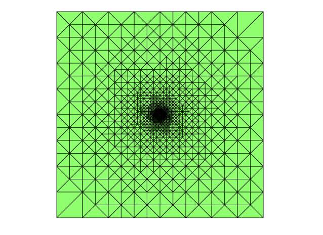
Figure 1: Kellogg problem: final mesh.

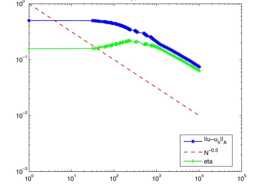
Figure 2: Error comparison.

With $f=0$ for the Kellogg problem, we note that $\eta_{\sigma}=0$, therefore, $\eta=\eta_{\rho}$. Even though for the nonconforming error we recover a gradient that is not curl free, (thus we were not be able to prove that the reliability constant is $1$ for the nonconforming error) the numerics still shows the behavior of asymptotic exactness, i.e., when the mesh is fine enough the efficiency index is close to $1$.

For the second test problem, we consider a Poisson L-shaped problem that has a nonzero conforming error $\eta_{\sigma}$. On the L-shaped domain $\Omega=[-1,\,1]^{2}\setminus[0,\,1]\times[-1,\,0]$, the Poisson problem ($A=I$) has the following exact solution

$$u(r,\theta)=r^{2/3}\sin((2\theta+\pi)/3)+r^{2}/2.$$

The numerics is based on the Crouziex-Raviart finite element approximation. With the relative error being less than $0.75\%$, the final mesh generated the adaptive mesh refinement algorithm is depicted in Figure 4. Clearly, the mesh is relatively centered around the singularity (origin). Comparison of the true error and the estimator is presented in Figure 4. It is obvious that the error converges in an optimal order (very close to $-1/2$) and that the efficiency index is very close to $1$ for all iterations.

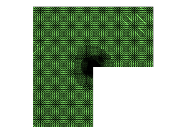
Figure 3: L-shape problem: final mesh.

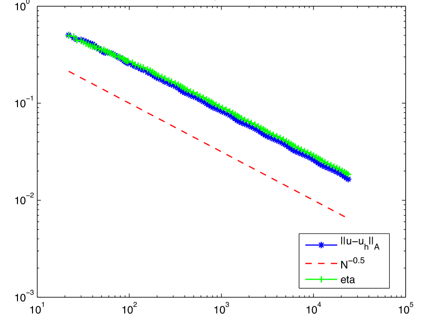
Figure 4: Error comparison.

References

• [1] M. Ainsworth, Robust a posteriori error estimation for nonconforming finite element approximation, SIAM J. Numer. Anal., 42:6 (2005), 2320–2341.
• [2] M. Ainsworth, A posteriori error estimation for discontinuous Galerkin finite element approximation, SIAM J. Sci. Comput., 30 (2007), 189–204.
• [3] M. Ainsworth and J. T. Oden, A unified approach to a posteriori error estimation using element residual methods, Numer. Math., 65 (1993), 23–50.
• [4] M. Ainsworth and R. Rankin, Fully computable bounds for the error in nonconforming finite element approximations of arbitrary order on triangular elements, SIAM J. Numer. Anal., 46 (2008), 3207–3232.
• [5] Á. Baran and G. Stoyan, Gauss-Legendre elements: A stable, higher order non-conforming finite element family, Computing, 79 (2007), 1–21.
• [6] M. Ainsworth and J. T. Oden, A Posteriori Error Estimation in Finite Element analysis, John Wiley & Sons, Inc., 2000.
• [7] C. Bernardi and R. Verfürth, Adaptive finite element methods for elliptic equations with non-smooth coefficients, Numer. Math., 85 (2000), 579–608.
• [8] R. Becker, D. Capatina, and R. Luce, Local flux reconstructions for standard finite element methods on triangular meshes, SIAM Journal on Numerical Analysis, 54 (2016), 2684–2706.
• [9] D. Boffi, F. Brezzi, and M. Fortin, Mixed Finite Element Methods and Applications, Springer, Heidelberg, 2013.
• [10] D. Braess, Finite Elements: Theory, Fast Solvers and Applications in Solid Mechanics, 3rd ed., Cambridge University Press, Cambridge, UK, 2007.
• [11] D. Braess, T. Fraunholz, and R. H. Hoppe, An equilibrated a posteriori error estimator for the Interior Penalty Discontinuous Galerkin method, SIAM J. Numer. Anal., 52 (2014), 2121–2136.
• [12] D. Braess and J. Schöberl, Equilibrated residual error estimator for edge elements, Math. Comp., 77 (2008), 651–672.
• [13] D. Braess, V. Pillwein, and J. Schöberl, Equilibrated residual error estimates are p-robust, Comput. Methods Appl. Mech. Engrg., 198 (2009), 1189–1197.
• [14] D. Cai, Z. Cai, and S. Zhang, Robust equilibrated a posteriori error estimator for higher order finite element approximations to diffusion problems, Numer. Math., 144:1 (2020), 1–21.
• [15] Z. Cai, C. He, and S. Zhang, Discontinuous finite element methods for interface problems: robust a priori and a posteriori error estimate, SIAM. J. Numer. Anal., 55 (2017), 400–418.
• [16] Z. Cai and S. Zhang, Recovery-based error estimator for interface problems: Mixed and nonconforming elements, SIAM. J. Numer. Anal., 48:1 (2010), 30–52.
• [17] Z. Cai and S. Zhang, Robust equilibrated residual error estimator for diffusion problems: conforming elements, SIAM J. Numer. Anal., 50 (2012), 151–170.
• [18] Y. Cha, M. Lee, and S. Lee, Stable nonconforming methods for the Stokes problem, Appl. Math. Comput., 114 (2000), 155–174.
• [19] M. Crouzeix and P. A. Raviart, Conforming and non-conforming finite element methods for solving the stationary Stokes equations, RAIRO Anal. Numer., 7 (1977), 33–75.
• [20] P. Destuynder and B. Métivet, Explicit error bounds for a nonconforming finite element method, SIAM J. Numer. Anal., 35:5 (1998), 2099–2115.
• [21] P. Destuynder and B. Métivet, Explicit error bounds in a conforming finite element method, Math. Comp., 68 (1999), 1379-1396.
• [22] L. Demkowicz and M. Swierczek, An adaptive finite element method for a class of variational inequalities, in Selected Problems of Modern Continuum Theory, Bologna, June 3-6, 1987, 11-28.
• [23] E. Alexandre, N. Serge and V. Martin, An accurate H (div) flux reconstruction for discontinuous Galerkin approximations of elliptic problems, Comptes Rendus Mathematique, 345 (2007), 709–712.
• [24] M. Fortin and M. Soulie, A non-conforming piecewise quadratic finite element on triangles, International Journal for Numerical Methods in Engineering, 19 (1983), 505–520.
• [25] R.B. Kellogg, On the Poisson equation with intersecting interfaces, Appl. Anal., 4 (1975), 101–129.
• [26] K.Y. Kim, Flux reconstruction for the $P^{2}$ nonconforming finite element method with application to a posteriori error estimation, Appl. Numer. Math., 62 (2012), 1701–1717.
• [27] P. Ladevèze and D. Leguillon, Error estimate procedure in the finite element method and applications, SIAM J. Numer. anal., 20:3 (1983), 485–509.
• [28] L. D. Marini, An inexpensive method for the evaluation of the solution of the lowest order Raviart–Thomas mixed method, SIAM J. Numer. Anal., 22 (1985), 493–496.
• [29] J. T. Oden, L. Demkowicz, W. Rachowicz and T. A. Westermann, Toward a universal h-p adaptive finite element strategy, Part 2. A posteriori error estimation, Comput. Methods Appl. Mech. Engrg., 77 (1989), 113-180.
• [30] M. Petzoldt, a posteriori error estimators for elliptic equations with discontinuous coefficients, Adv. Comp. Math., 16 (2002), 47–75.
• [31] W. Prager and J. L. Synge, Approximations in elasticity based on the concept of function space, Quart. Appl. Math., 5 (1947), 286–292.
• [32] G. Stoyan and Á. Baran, Crouzeix-Velte decompositions for higher-order finite elements, Comput. Math. Appl., 51 (2006), 967–986.
• [33] T. Vejchodský, Guaranteed and locally computable a posteriori error estimate, IMA J. Numer. Anal., 26 (2006), 525–540.
• [34] R. Verfürth, A note on constant-free a posteriori error estimates, SIAM J. Numer. Anal., 47 (2009), 3180–3194.