AC magnetic response of highly nonlinear soliton lattice in a monoaxial chiral helimagnet
Abstract
We present the theory of nonlinear ac magnetic response for the highly nonlinear regime of the chiral soliton lattice. Increasing of the dc magnetic field perpendicularly to the chiral axis results in crossover inside the phase, when nearly isolated -kinks are partitioned by vast ferromagnetic domains. Assuming that each of the kink reacts independently from the other ones to the external ac field, we demonstrate that internal deformations of such a kink give rise to the nonlinear response.
pacs:
Valid PACS appear hereI Introduction
Measurements of nonlinear ac magnetic response can provide extremely useful information for understanding physical properties of various magnetic compounds. This powerful magnetic diagnostics is conventionally used to elucidate a dynamics of magnetic domains in ferromagnets Sato1981 in addition to allowing the determination of the phase transition temperature Hashimoto1973 . This experimental technique has applications in studies of low-field magnetic hysteresis of ferromagnetic Rayleigh1887 ; Milstein1975 and helimagnetic materials Mito2010 ; Mito2015 , nonlinear response in ferroelectrics Ishibashi1994 and molecule-based magnets with structural chirality Mito2009 ; Mito2012 . Another broad research area involves studies of nonlinear susceptibility in the vicinity of spin glass transition temperature Suzuki1977 ; Miyako1979 ; Fujiki1981 . A chirality driven mechanism due to fluctuations of a dynamical noncollinear spin order variable, which defined as a vector product of two nearest-neighbor lattice spins, was proposed to explain new universality classes of experimentally observed spin-glass critical phenomena Kawamura1992 ; Maleyev2002 ; Maleyev2004 ; Kawamura2010 ; Campbell2010 .
Recent investigations of chiral magnets have become a new landmark of the nonlinear response applications. These materials comprise both the chirality of critical fluctuations, such as in the case of MnSi Grigoriev2005 ; Papas2011 , and the ac magnetic response of magnetic domains found, for example, in CrNb3S6 Tsuruta2016 . In the latter case, the phase diagram of the chiral helimagnet as a function of temperature and a dc magnetic field was constructed by means of the ac magnetic susceptibility measurements. It was revealed that when the ac response consists of a giant third-order harmonic component () along with a first-order part () at the transition between the chiral helimagnetic (CHM) state to the paramagnetic (PM) state. The non-zero dc field applied perpendicular to the helical axis transforms the CHM state in favor of the chiral soliton lattice (CSL) state. At small , ferromagnetic regions are poorly expressed against the predominant magnetic helicoidal order. For this regime, it was found that the is drastically suppressed, i.e. the transition between the CSL and the PM states is characterized only by a linear magnetic response. At higher dc fields, the ferromagnetic domains start to grow that allows the CSL state to be viewed as a regular arrangement of 2-kinks in the ferromagnetic background. With increasing temperature, this CSL state is transformed into the forced ferromagnetic (FFM) state, and eventually the PM state is reached. The transition between the CSL state and the FFM states is again accompanied by a large as well as a complex , whereas the FFM-PM transition gives rise a linear magnetic response without any energy loss. These data reported by Mito al. Tsuruta2016 were supplemented by a comprehensive study made by Clements at al. Clements2018 . They could trace the dc magnetic field dependence of the ac magnetic response for the first five harmonic components and have amply demonstrated a presence of the noticeable component as the ferromagnetic-domain-rich CSL evolves into the FFM state. In small ac-fields, the is connected to the breaking of the time inversion symmetry, and the large signal reflects the presence of spontaneous magnetization Hashimoto1973 . The , in contrast, is associated with the microscopic breaking of spatial symmetry of magnetic moments Mito2009 , thereby confirming the presence of the ferromagnetic domains in the highly nonlinear CSL state.
The peculiarities discovered in the nonlinear response are closely linked to the phase diagram of the chiral helimagnet CrNb3S6, detailed structure thereof is still actively debated. The nature of the possible phase transitions has been addressed both experimentally and theoretically. The dc magnetization and magnetic entropy change measurements Ghimire2013 ; Clements2017 testify apparently a second-order phase transition to the FFM state at magnetic fields above the critical field of the incommensurate-commensurate (IC-C) phase transition. At moderate and low magnetic fields the onset of the chiral IC phase was detected, including crossover between the nonlinear and highly nonlinear regions of the CSL state along with complementary crossover between the CHM and CSL states. These investigations also confirm the existence of the weakly nonlinear CSL and the concurrent disappearance of the CHM phase for small non-zero applied fields in temperature region above and below the Curie temperature 130.7 K. A possibility of first-order behavior at the phase transition in small magnetic fields were also argued. The metamagnetic crossover from the weakly nonlinear to the highly nonlinear CSL regime has been verified by measurements of magnetoresistance Togawa2013 . The theoretical studies by Laliena et al. Laliena2016 ; Laliena2017 predict a transition line between the highly nonlinear CSL and the FFM states at low temperature and high dc fields as being of second-order (continuous) nucleation type transition Gennes1975 . The boundary between the CHM and the PM state may be categorized as the second-order instability type transition Izyumov1985 according to de Gennes classification. The second-order line sections are separated by a line of first-order transitions with two tricritical points as a terminus at intermediate temperatures and magnetic fields. Experimental validation of these tricritical points remains controversial Han2017 . Another examples of the nucleation type transition are the transition at the lower critical field of type-II superconductors and the cholesteric-to-nematic transition in liquid crystals. The former analogy was discussed in Refs. Shinozaki2019 ; Masaki2020 , where a similarity of surface barrier between the monoaxial chiral helimagnet and type-II superconductors was pointed out.
In our work we present the theory of nonlinear ac magnetic response for the highly nonlinear regime of the chiral soliton lattice. The state emerging as a result of crossover under increasing the dc magnetic field perpendicularly to the chiral axis may be regarded as a regular arrangement of nearly isolated kinks partitioned by vast ferromagnetic domains. It is separated from the FFM state by the nucleation type continuous transition and may be modeled as particles that repel each other by a force which decay exponentially as a distance between the kinks increases Rubinstein1970 . Then, it is appropriate to assume that each of the kinks reacts independently from the other ones to the external ac field. We argue that the appearance of high-order harmonics and phase shifts is related to quasi-localized excitations triggered by internal deformations of the separate kink.
To provide support for the picture presented above we formulate a model of the magnetic soliton lattice relevant for the chiral helimagnet CrNb3S6 and explain how crossover between the weakly and highly nonlinear CSL regimes originates from Fourier decomposition of the CSL configuration. Furthermore, we find spectrum of Gaussian fluctuations of a single kink, thereby specifying its internal deformations. Using the spectrum, a Lagrangian formalism based on the collective coordinate method Book2015 ; Kishine2012 ; Kishine2016 is developed to describe kink dynamics driven by an external ac magnetic field. Solving of the corresponding dynamical equations is reduced to a challenge how to get periodic (Floquet) solutions. We apply the algorithm elaborated by Erugin Erugin to successfully overcome the problem and use the periodic solutions to recover higher-order harmonic components of magnetization together with related phase shifts. Our analysis reveals that the order parameter which characterizes the second order phase transition of the nucleation type, namely a density of kinks, has a crucial role to play in hierarchy of these higher-order harmonic components. This allows to establish the limits of our theory and predicts the onset of the linear response regime while approaching the FFM phase boundary.
This paper is organized as follows. In Sec. II, we describe the model and summarize key details of the ground state and the excitations of the highly nonlinear CSL state. Here, the Lagrangian formalism to describe dynamics of a single kink is presented. In Sec. III, the periodic solution of the dynamical equations is looked for which is used to derive higher order harmonics of nonlinear magnetic response. The conclusions are given in Sec. IV.
II Model
The layered structure of CrNb3S6 consists of 2H-type planar NbS2 with the Cr atoms intercalated between the planes and belongs to the non-centrosymmetric hexagonal space group P6322 Togawa2016 . The localized moments of the Cr3+ ions (the spin ) are oriented in the crystallographic ab plane and exhibit strong single-ion anisotropyMoriya1982 ; Miyadai1983 . As has been repeatedly proven the qusi-1D model of the chiral soliton lattice Dzyaloshinskii1964 explains property of the compound beautifully that was amply confirmed by Togawa et al. via the Lorentz microscopy experiments Togawa2012 .
In the continuum approximation, the monoaxial chiral helimagnet is described by the Hamiltonian, , with the density
| (1) |
where is the lattice constant and the semiclassical spin
is specified by the polar coordinates. Here, is the strength of the nearest-neighbor ferromagnetic exchange coupling. The mono-axial DM vector directed along the -axis is parametrized by the constant . To stabilize the CSL state, a static magnetic field , measured in units , is applied perpendicularly to the -axis.
The CSL ground state is given by and , where the dimensionless coordinate is introduced with . The is the Jacobi amplitude function depending on the elliptic modulus (). The modulus is determined by minimizing an energy that gives , where , and the CSL spatial period, , with and being the elliptic integrals of the first and second kind, respectively.
The CSL undergoes a continuous transition to the forced ferromagnetic state above the critical field
| (2) |
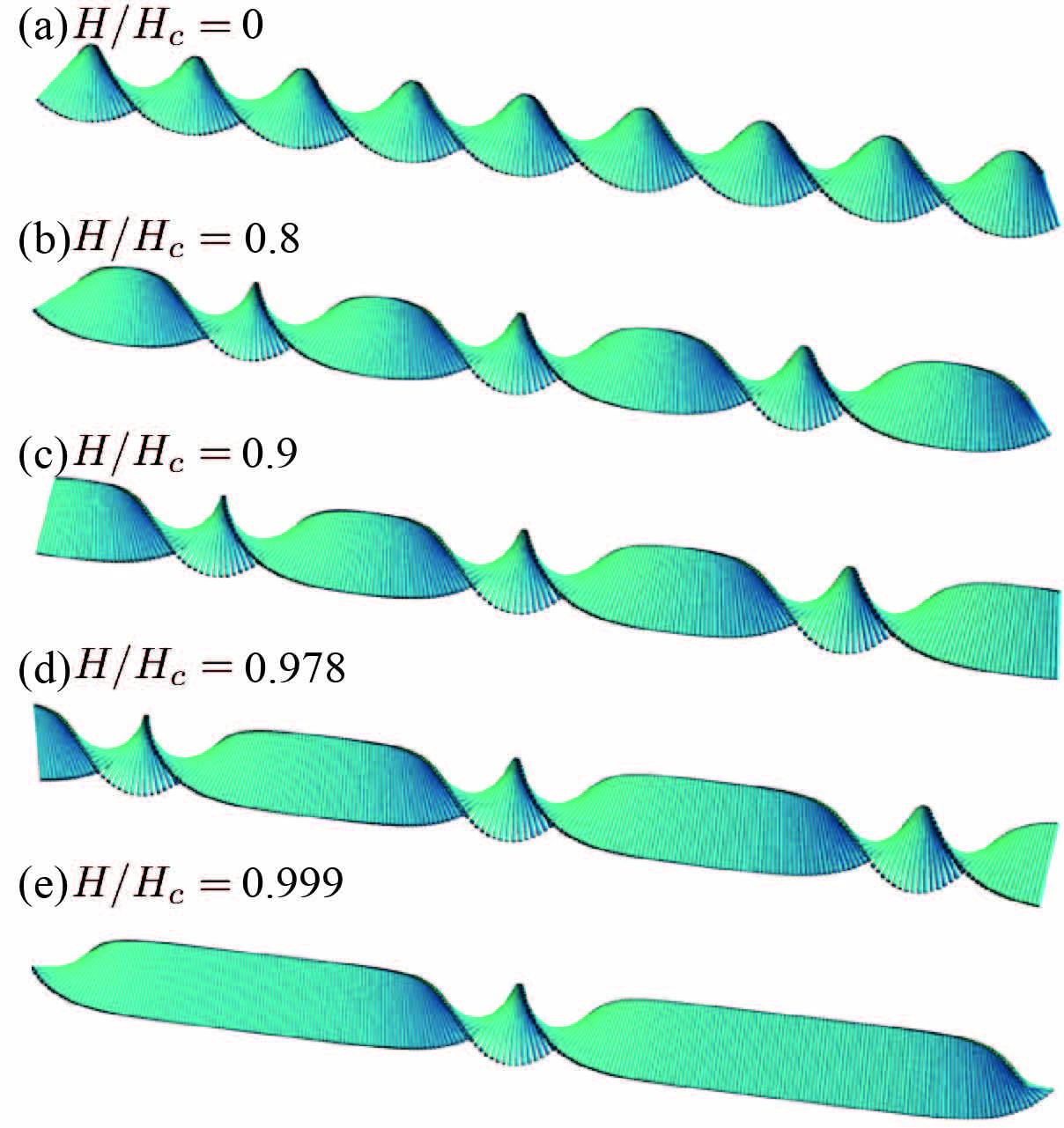
attained as . The evolution of the CSL upon increasing is schematically shown in Fig.1. It should be recognized that a nonlinear magnetic structure becomes conspicuous only in the vicinity of the critical field .
To see the evolution of the nonlinearity in a more quantitative manner, let us Fourier decompose the CSL configuration,
| (3) | ||||
| (4) |
where denotes the complete elliptic integral of the first kind with the complementary elliptic modulus . We note that .
From Eqs. (3) and (4), we obtain the Fourier decomposed weights for the ferromagnetic component
| (5) |
and the spatially modulated components,
| (6) |
The ratio is an indicator of nonlinearity in the CSL structure. The weight corresponds to the harmonic modulation of the helix, while the weight indicates an evolution of the ferromagnetic domains. The dominance of over means the onset of nonlinearity. In Fig. 2(a), we show the field dependence of the and . It is seen that exceeds the unity at . This value determines crossover between the linear and the higly nonlinear CSL regimes.Laliena2017
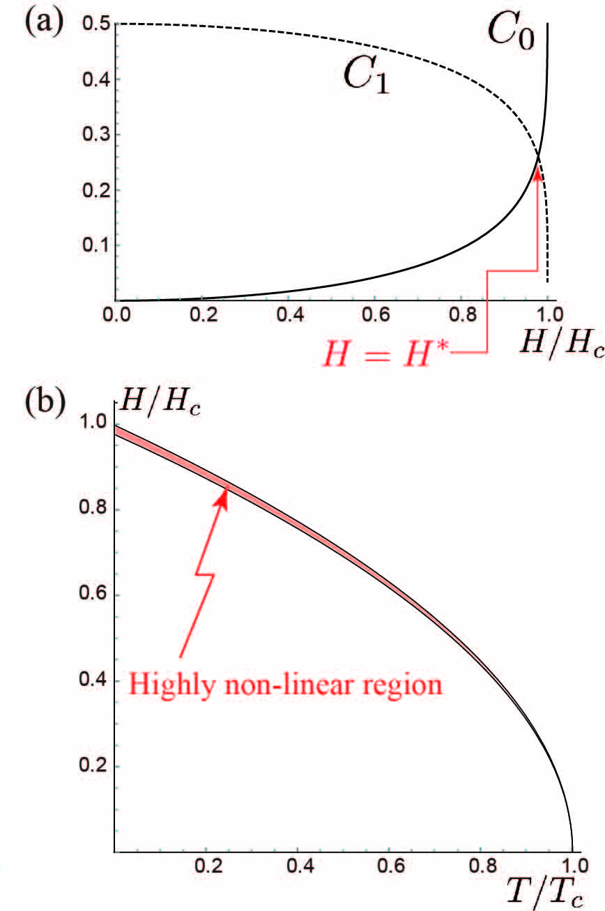
To gain insight into the appearance of the crossover line on the field-temperature phase diagram, we replace with a simple mean-field form having the temperature dependence, , where denotes the transition temperature at zero field. Inserting this form into Eq. (2), we acquire the temperature dependent critical field . On the other hand, it can be assumed that the crossover value is independent on temperature that brings forth the conceptual phase diagram shown in Fig. 2(b). We note that the highly nonlinear regime occupies a quite narrow region bounded by .
II.1 Spectrum of fluctuations
Below, we thoroughly discuss fluctuations around the soliton lattice ground state,
| (7) | ||||
| (8) |
By expanding the Hamiltonian (1) up to the second order with respect to the and , we obtain , where
| (9) |
Here, the linear differential operators are given by
| (10) |
and
| (11) |
with
| (12) |
being the energy gap function of the -mode originated from the DM interaction. Here, is the wave number of the CSL structure.
The physical situation of a single kink inside of a ferromagnetic matrix corresponds to a highly nonlinear regime achieved when . In this case, the CSL solution degenerates into
| (13) |
where with being the width of the kink localization (see the inset of Fig.4).
Figure 3 illustrates the potentials for the -fluctuations, sech, and the - fluctuations, sechsech, where we present additionally the gap function, , at .
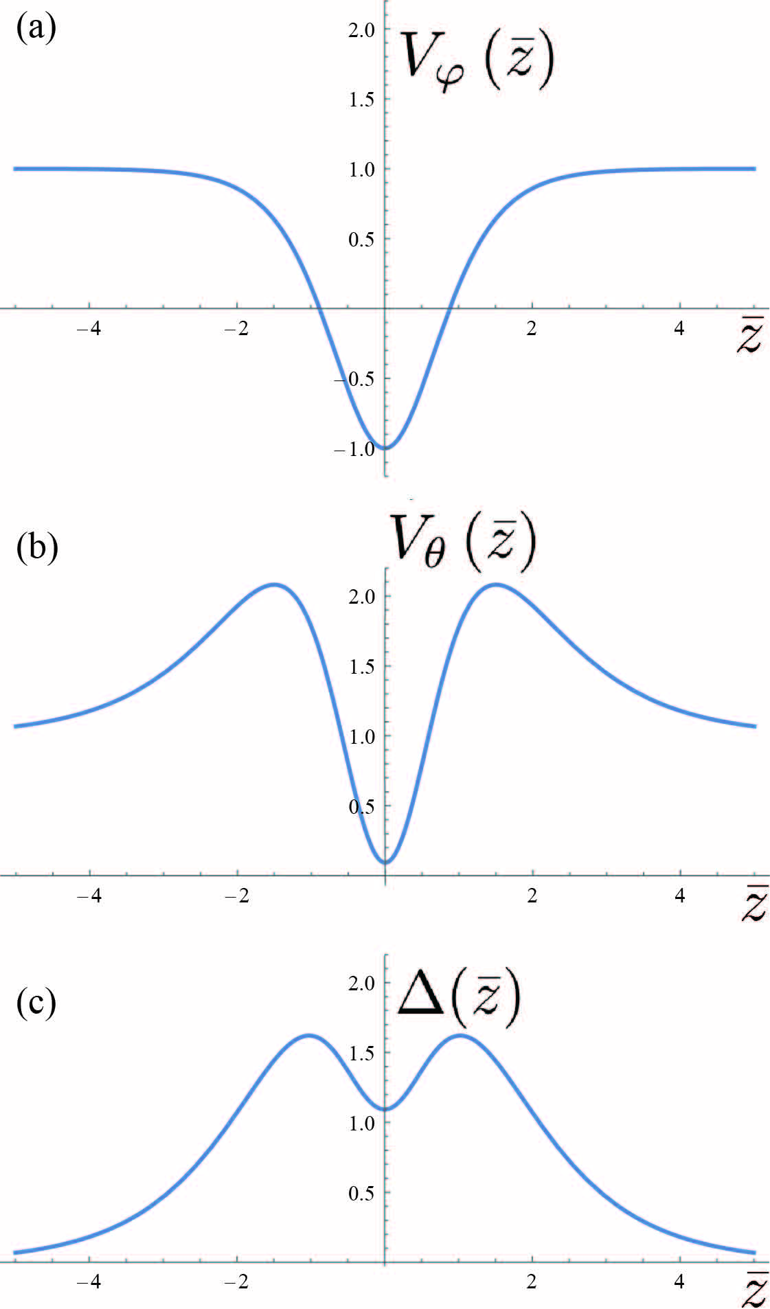
The Schrödinger-type operator involves the Pöschl-Teller potential defined by with the particular value . For further analysis, the most important being a presence of the single bound state with the eigenvalue (zero mode) Kishine2010 .
Unfortunately, the operator does not permit a similar treatment. However, it may be shown through the WKB formalism (see Appendix A) that there is a quasi-localized state with the energy , . By using Eqs.(79,80) we get provided . Numerov algorithm yields . We neglect henceforth the tunneling process giving a finite width of the state.
II.2 Lagrangian
Our target is to obtain equations of motion of the isolated kink in the ferromagnetic surrounding based on the fluctuation spectra discussed above.
The Lagrangian density includes three terms,
| (16) |
such as the kinematic part associated with the Berry phase
| (17) |
the part related to the kink energy,
| (18) |
and the Zeeman coupling with the oscillating field, , of the strength and the frequency ,
| (19) |
Integration runs over the interval that has the kink at the center.
In the method of collective coordinates the dynamics is fully described by two variables, the center-of-mass position and the out-of-plane quasi-zero mode coordinate
| (20) |
| (21) |
To obtain equations of motion in the context of the collective coordinates we expand the Lagrangian (16) in terms of and , which are assumed to be small as long as the ac field is weak.
In this way, we get
| (22) |
where
| (23) | ||||
| (24) | ||||
| (25) |
and it is taken into consideration that the sliding coordinate corresponds to the zero mode of -excitations with . On the other hand, the -excitations acquire a finite energy gap .
The equations of motion for the collective coordinates are then given by
| (26) |
III Floquet solution and nonlinearity
III.1 Floquet solution
To find a Floquet solution of these equations of motion it is convenient to define the integral matrix composed from two linearly independent solutions
| (27) |
Then, the system (26) may be recast into the form
| (28) |
where ,
with
| (29) | ||||
| (30) | ||||
| (31) |
Here, the time is introduced. It is to be noted that , , and are inversely proportional to .
A way of constructing Floquet solution of Eq. (28) is explained in the Appendix B. This method is based on the fact that in the representation of the integral matrix
| (32) |
the and may be expanded as the series with respect to the small parameter , that appears in the coefficients of the system (28). In our analysis the series are limited to third order
| (33) |
| (34) |
Following the procedure set out in Appendix C one may find consistently and [see, Eqs.(85,86)]. The explicit forms of and are originated from Eqs. (88,87) and Eq.(89), respectively,
| (35) |
| (36) |
Reiterating steps of the algorithm for terms of second and third orders (see Appendix C for details) we obtain the matrix
| (37) |
It has purely imaginary characteristic numbers that yields
| (38) |
with
and the integral matrix turns out to be oscillatory as a result.
By carrying out direct calculation of Eq. (32) and ignoring a frequency shift to the value , we get eventually the first pair of the Floquet solution
| (39) |
| (40) |
Similarly, we find the second pair
| (41) |
| (42) |
which is the physical solution consistent with the initial condition , . Bearing in mind that if is the normalized integral matrix at the point , i.e. , then every other integral matrix can be expressed in the form , where is a constant matrix. Therefore, transition to an arbitrary kink position is achieved by the matrix .
III.2 Magnetization
The resultant magnetization is originated from dependence on the collective coordinates
| (43) |
where is the magnetization amplitude.
Performing expansion in powers of right up to third order (), we obtain the fluctuation part,
| (44) |
where
| (45) | ||||
| (46) | ||||
| (49) | ||||
| (52) |
It follows on parity grounds that and , note aslo that and .
By plugging the solutions (41,42) obtained earlier in (44) and neglecting higher-order terms the magnetization as function on time may be presented as follows
| (53) |
Here, the th-harmonic components, , are given by
| (54) | ||||
| (55) | ||||
| (56) |
We note that are proportional to , while to , since , , and are inversely proportional to .
The expressions for
| (57) |
| (58) |
and determine the phase delay of each against the ac-field.
Given the characteristic length of the “kink localization”, , we take the size of the system as
| (59) |
where measures how large the whole system size is as compared with the kink width. Larger corresponds to more sparse distribution of the kinks. Then, , and obey the following scaling laws with respect to ,
| (60) | ||||
| (61) | ||||
| (62) |
where we used (see Ref. Kishine2010 ) and . We note the parameters and has the same dependence on with and , respectively.
By using the values for CrNb3S6 as , K (or J), m. As for the ac magnetic field, we follow Ref. Tsuruta2016 and take Oe (then J) and Hz (then J). These vales lead to order-of-magnitude estimate,
| (63) | ||||
| (64) | ||||
| (65) |
Plugging them into Eqs. (54-56), we see that the harmonic components obey the scaling laws with respect to as
| (66) | ||||
| (67) | ||||
| (68) |
We show the -dependence of in Fig. 4(a). By choosing the characteristic length per the kink, , as , we obtain the proportion close to that observed in the experiment , and . The corresponding phase shifts are and .
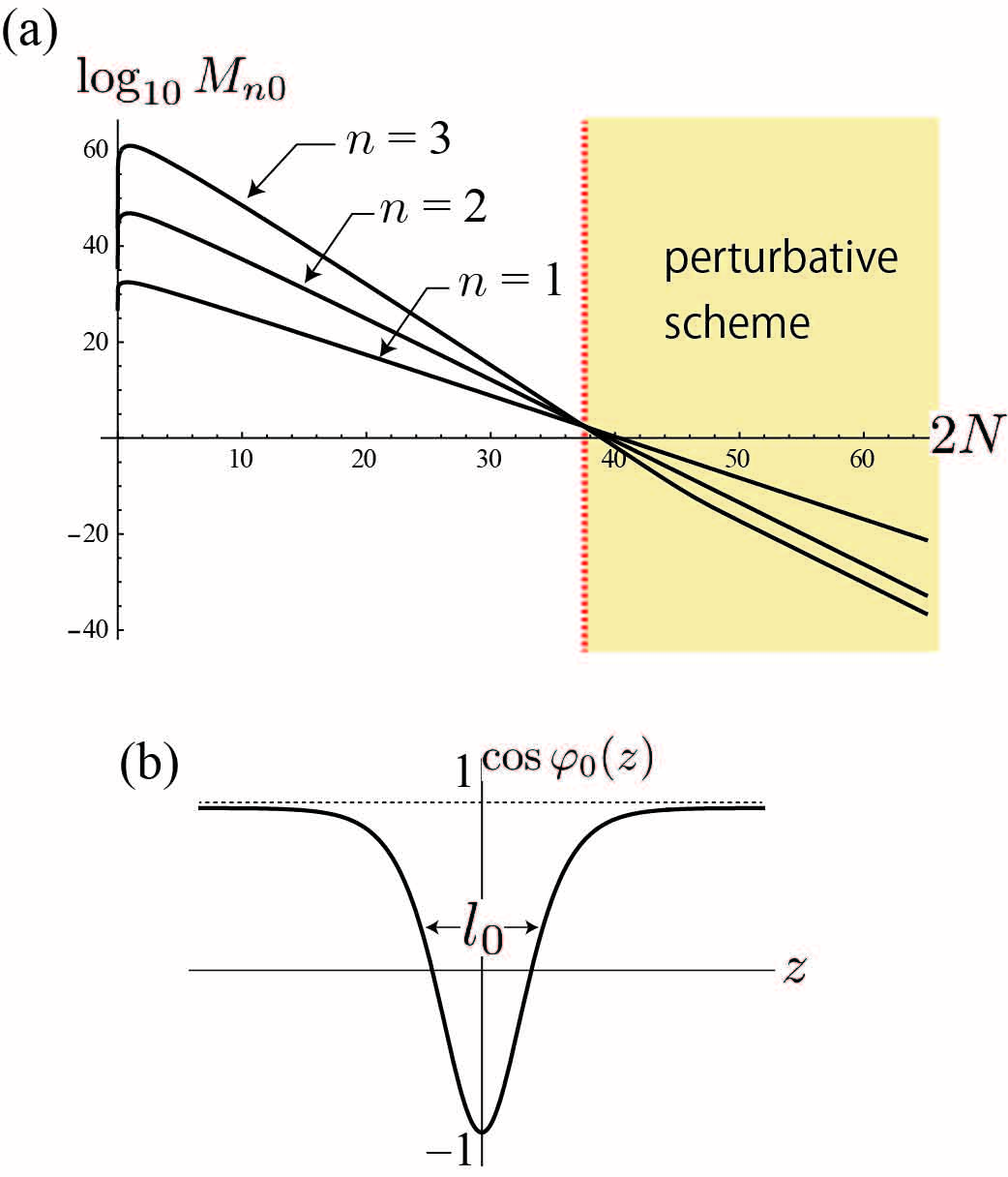
It is seen that as functions of , the amplitudes of higher harmic contributions, and dominate for smaller , which indicates that the perturbative scheme [expansions given in Eqs. (33) and (34)] breaks down. Because larger means lower kink density, our scheme works for the regime of smaller kink density specified by . This condition is consistent with the situation where the highly non-linear regime is near the boundary of the nucleation transition [see Fig. 2(b)].
IV Conclusion and discussions
The accumulated data on nonlinear response in CrNb3S6 provide exciting challenges that need to be treated theoretically. This task is closely linked with a general issue of emergence of slow dynamics from high energy processes Fukuyama2017 . In our study, we explain the origin of this phenomenon in the regime of highly nonlinear soliton lattice by internal deformations of separate -kinks driven by an external ac magnetic field. We demonstrate that the emergence of higher-order harmonics takes place in a narrow range of dc fields when there is an optimal distance between the kinks. At lower distances that corresponds to high density of the kinks our analysis based on a perturbative scheme becomes irrelevant. For larger lengths, i.e. small kink density, contribution of the higher-order harmonics is negligible and we have linear magnetic response in the vicinity of the phase transition into the state of forced ferromagnetism.
Note that temperature effects related both with the nonlinear response and behavior of the chiral soliton lattice as a wholeKrumhansl1975 ; Gupta1976 ; Shinozaki2016 remain beyond our treatment. The presented theory nevertheless may be exploited in addressing of second-order phase transitions of the nucleation type.
Acknowledgements.
The authors would like to express special thanks to Profs. Masaki Mito, Manh-Huong Phan, David Mandrus and Hidetoshi Fukuyama for very informative discussions during various stages. The authors also thank Victor Laliena, Javier Campo, and Yusuke Kato for fruitful discussions. This work was supported by a Grant-in-Aid for Scientific Research (B) (No. 17H02923) from the MEXT of the Japanese Government. A.S.O. acknowledges funding by the Foundation for the Advancement of Theoretical Physics and Mathematics BASIS Grant No. 17-11-107, and by Act 211 Government of the Russian Federation, contract No. 02.A03.21.0006. A.S.O. thanks also the Ministry of Education and Science of the Russian Federation, Project No. 3.2916.2017/4.6.Appendix A WKB method for
Below, we find the quasi-stationary levels of a particle in the symmetrical potential shown in Fig. 5 following a general scheme outlined in Ref. Haar1964 .
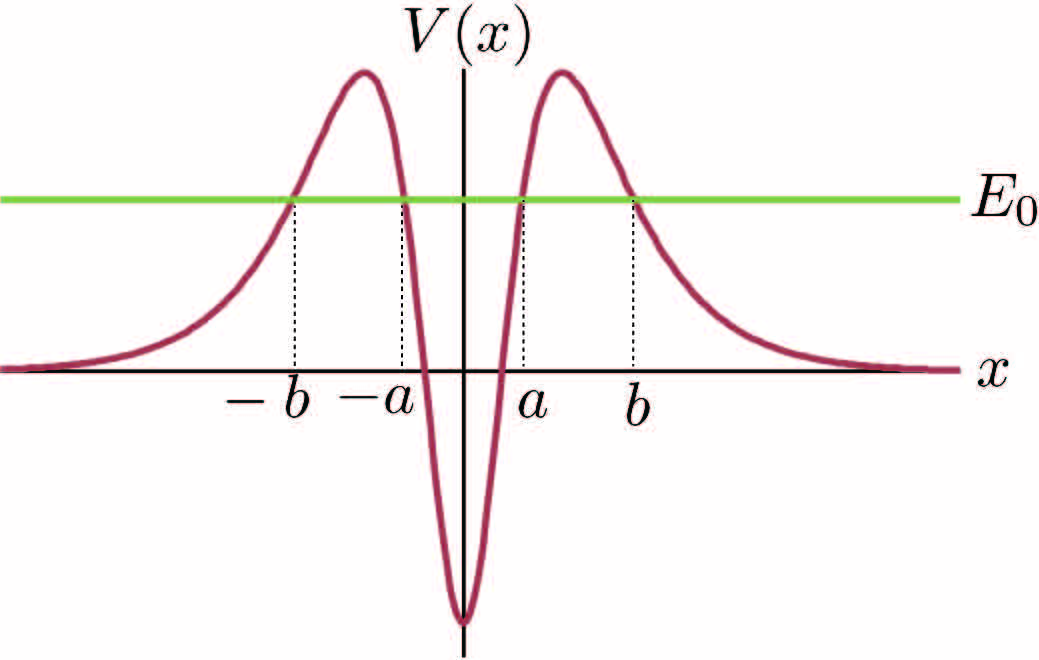
In the region we have a wave which goes to ,
| (69) |
where is a constant and is a momentum of the particle. In the region we obtain
| (70) |
In the region we get
| (71) |
In the region
| (72) |
In the region we find
| (73) |
An absence of a wave coming from yields
| (74) |
Provided , we obtain
| (75) |
where is a non-negative integer.
The quasi-stationary levels and their width are given by
| (76) |
where is the potential, is the mass of the particle, and
| (77) |
Here, is the angular frequency of the classical motion in a separate well,
To find we consider the Schroedinger-like equation
| (78) |
with .
The energy of the quasi-localized state may found from (76) at ,
| (79) |
where the upper limit of integration is related with the
| (80) |
that results in .
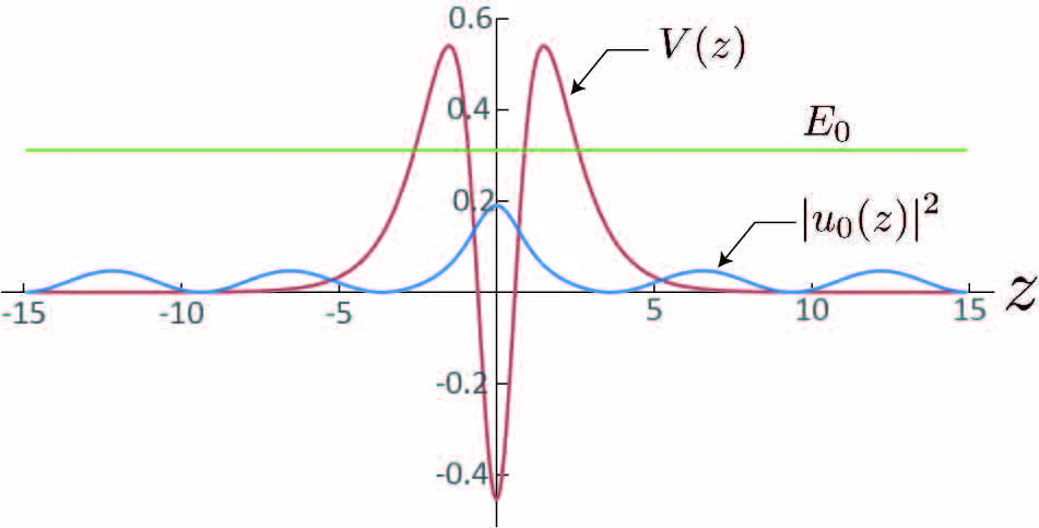
In Fig. 6 the numerical solution via the Numerov’s algorithm is shownLandau2008 . The corresponding value is .
Appendix B Erugin’s method
We consider a system of the form
| (81) |
where are -th order matrices that are continuous and periodic with period , is a small parameter.
The integral matrix of Eq.(81) normalized at the point can be expressed as a series
| (82) |
with , at .
It can be shown (see Ref. Erugin ) that the integral matrix, giving Floquet solution, can be represented in the form
| (83) |
where is the real constant matrix and is periodic with the period .
According to the general theory we have these quantities in the form of the series in powers of ,
| (84) |
The recipe for finding of the and may be explained as follows. Firstly, we define
| (85) |
and
| (86) |
We can now calculate the periodic matrix with period
| (87) |
Then, may be found from
| (88) |
After all, we obtain
| (89) |
Appendix C Matrices and for
Below we result explicitly the matrices and , , necessary to build a Floquet solution.
References
- (1) T. Sat and Y. Miyako, J. Phys. Soc. Jpn. 51, 1394 (1981).
- (2) T. Hashimoto, A. Sato, and Y. Fujiwara, J. Phys. Soc. Jpn. 35, 81 (1973).
- (3) L. Rayleigh, Philos. Mag. 23, 225 (1887).
- (4) F. Milstein, J.A. Baldwin, Jr., and M. Rizzuto, J. Appl. Phys. 46, 4002 (1975).
- (5) M. Mito, S. Tominaga, Y. Komorida, H. Deguchi, S. Takagi, Y. Nakao, Y. Kousaka, and J. Akimitsu, J. Phys.: Conf. Ser. 215, 012182 (2010).
- (6) M. Mito, H. Matsui, K. Tsuruta, H. Deguchi, J. Kishine, K. Inoue, Y. Kousaka, S. Yano, Y. Nakao, and J. Akimitsu, J. Phys. Soc. Jpn. 84, 104707 (2015).
- (7) Y. Ishibashi and H. Orihara, Ferroelectrics 156, 185 (1994).
- (8) M. Mito, K. Iriguchi, H. Deguchi, J. Kishine, K. Kikuchi, H. Ohsumi, Y. Yoshida, and K. Inoue, Phys. Rev. B 79, 012406 (2009).
- (9) M. Mito, K. Iriguchi, H. Deguchi, J. Kishine, Y. Yoshida, and K. Inoue, J. Appl. Phys. 111, 103914 (2012).
- (10) M. Suzuki, Prog. Theor. Phys. 58, 1151 (1977).
- (11) Y. Miyako, S. Chikazawa, T. Saito, and Y.G. Yuochunas, J. Phys. Soc. Jpn. 46, 1951 (1979).
- (12) S. Fujiki and S. Katsura, Prog. Theor. Phys. 65, 1130 (1981).
- (13) H. Kawamura, Phys. Rev. Lett. 68, 3785 (1992).
- (14) S.V. Maleyev, Physics-Uspekhi 45, 569 (2002).
- (15) S.V. Maleyev, Physica B 297, 67 (2001); 345, 119 (2004).
- (16) H. Kawamura, J. Phys. Soc. Jpn. 79, 011007 (2010) and references therein.
- (17) I.A. Campbell and D.C.M.C. Petit, J. Phys. Soc. Jpn. 79, 011006 (2010) and references therein.
- (18) S.V. Grigoriev, S.V. Maleyev, A.I. Okorokov, Yu.O. Chetverikov, R. Georgii, P. Böni, D. Lamago, H. Eckerlebe, and K. Pranzas, Phys. Rev. B 72, 134420 (2005).
- (19) C. Pappas, E. Lelièvre-Berna, P. Bentley, P. Falus, P. Fouquet, and B. Farago, Phys. Rev. B 83, 224405 (2011).
- (20) K. Tsuruta, M. Mito, H. Deguchi, J. Kishine, Y. Kousaka, J. Akimitsu, and K. Inoue, Phys. Rev. B 93, 104402 (2016).
- (21) E. M. Clements, R. Das, M.-H. Phan, L. Li, V. Keppens, D. Mandrus, M. Osofsky, and H. Srikanth, Phys. Rev. B 97, 214438 (2018).
- (22) N.J. Ghimire, M.A. McGuire, D.S. Parker, B. Sipos, S. Tang, J.-Q. Yan, B.C. Sales, D. Mandrus, Phys. Rev. B 87, 104403 (2013).
- (23) E.M. Clements, R. Das, L. Li, P.J. Lampen-Kelley, M.-H. Phan, V. Keppens, D. Mandrus, and H. Srikanth, Scientific Reports 7, 1 (2017).
- (24) Y. Togawa, Y. Kousaka, S. Nishihara, K. Inoue, J. Akimitsu, A. S. Ovchinnikov, and J. Kishine, Phys. Rev. Lett. 111, 197204 (2013).
- (25) V. Laliena, J. Campo, and Y. Kousaka, Phys. Rev. B 94, 094439 (2016).
- (26) V. Laliena, J. Campo, and Y. Kousaka, Phys. Rev. B 95, 224410 (2017).
- (27) P. de Gennes, in Fluctuations, Instabilities, and Phase Transitions, edited by T. Riste, NATO ASI Series B Vol. 2 (Plenum, New York, 1975).
- (28) Y.A. Izyumov and V.M. Laptev, J. Mag. Mag. Mat. 51, 381 (1985).
- (29) H. Han, L. Zhang, D. Sapkota, N. Hao, L. Ling, H. Du, L. Pi, C. Zhang, D. Mandrus, and Y. Zhang, Phys. Rev. B 96, 094439 (2017).
- (30) M. Shinozaki Y. Masaki, R. Aoki, Y. Togawa, and Y. Kato, Phys. Rev. B 97, 214413 (2018).
- (31) Y. Masaki, arXiv:1912.12677.
- (32) J. Rubinstein, J. Math. Phys. 11, 258 (1970).
- (33) J. Kishine and A. S. Ovchinnikov, Solid State Phys. 66, 1 (2015).
- (34) J. Kishine, I. G. Bostrem, A. S. Ovchinnikov, and Vl. E. Sinitsyn, Phys. Rev. B 86, 214426 (2012).
- (35) J. Kishine, I. Proskurin, I. G. Bostrem, A. S. Ovchinnikov, and Vl. E. Sinitsyn, Phys. Rev. B 93, 054403 (2016).
- (36) N.P. Erugin, Linear Systems of Ordinary Differential Equations with Periodic and Quasi-Periodic Coefficients (Academic Press, New York and London, 1966).
- (37) Y. Togawa, Y. Kousaka, K. Inoue, and J. Kishine, J. Phys. Soc. Jpn. 85, 112001 (2016).
- (38) T. Moriya and T. Miyadai, J. Phys. Soc. Jpn. 42, 209 (1982).
- (39) T. Miyadai, K. Kikuchi, H. Kondo, S. Sakka, M. Arai, Y. Ishikawa, J. Phys. Soc. Jpn. 52, 1394 (1983).
- (40) I.E. Dzyaloshinskii, Zh. Eksp. Teor. Fiz. 46, 1420 (1964) [Sov. Phys. JETP 19, 960 (1964)]; Zh. Eksp. Teor. Fiz. 47, 992 (1964) [Sov. Phys. JETP 20, 665 (1965)].
- (41) Y. Togawa, T. Koyama, K. Takayanagi, S. Mori, Y. Kousaka, J. Akimitsu, S. Nishihara, K. Inoue, A.S. Ovchinnikov, and J. Kishine, Phys. Rev. Lett. 108, 107202 (2012).
- (42) J. Kishine and A. S. Ovchinnikov, Phys. Rev. B 81, 134405 (2010).
- (43) R.H. Landau, M.J. Páez, and C.C. Bordeianu, A Survey of Computational Physics (Princeton U.P., Princeton, NJ, 2008).
- (44) H. Fukuyama, J. Kishine and M. Ogata, J. Phys. Soc. Jpn. 86, 123706 (2017).
- (45) J. A. Krumhansl and J. R. Schrieffer, Phys. Rev. B 11, 3535 (1975).
- (46) N. Gupta and B. Sutherland, Phys. Rev. A 14, 1790 (1976).
- (47) M. Shinozaki1, S. Hoshino, Y. Masaki, J. Kishine, and Y. Kato, J. Phys. Soc. Jpn. 85, 074710 (2016).
- (48) D. ter Haar, Selected Problems in Quantum Mechanics (Infosearch Limited, London, 1964).