Work function, deformation potential, and collapse of Landau levels in strained graphene and silicene

Abstract

We perform a systematic ab initio study of the work function and its uniform strain dependence for graphene and silicene for both tensile and compressive strains. The Poisson ratios associated with armchair and zigzag strains are also computed. Based on these results, we obtain the deformation potential, crucial for straintronics, as a function of the applied strain. Further, we propose a particular experimental setup with a special strain configuration that generates only the electric field, while the pseudomagnetic field is absent. Then, applying a real magnetic field, one should be able to realize experimentally the spectacular phenomenon of the collapse of Landau levels in graphene or related two-dimensional materials.

I Introduction

One of the remarkable features of two-dimensional (2D) Dirac materials such as graphene and silicene is the formation of the relativisticlike Landau levels in a magnetic field. When in addition to the magnetic field the electric field is applied in the plane the spectacular phenomenon of Landau level collapse occurs. It consists of the merging of the Landau level staircase when the applied electric field reaches its critical value and the cyclotron frequency becomes zero Lukose et al. (2007); Peres and Castro (2007). The behavior of Landau levels in these materials can be controlled by tuning external magnetic and electric fields along with strain that effectively induces artificial electromagnetic fields Vozmediano et al. (2010); Amorim et al. (2016); Naumis et al. (2017).

The value of the strain-induced electric field is determined by the corresponding deformation potential that is present in the tight-binding description. In their turn the characteristics of this potential can be extracted from the strain dependence of the work function (WF). The relationship between the deformation potential and the WF can be determined accurately by both experiments and ab initio calculations. Here we quantitatively evaluate the deformation potential by ab initio calculation of the work function in the strained graphene and silicene. Combining these systematic ab initio calculations of the WF, the deformation potential, and the tight-binding model Hamiltonian, we propose the new experimentally feasible condition of Landau level collapse in graphene using strain.

(i) It is well known that the energies of relativistic Landau levels of graphene in a magnetic field $B$ applied perpendicular to the plane in the presence of an in-plane electric field $E$ are Lukose et al. (2007); Peres and Castro (2007)

$$E_{n}=\pm\Omega_{L}\sqrt{n}-\hbar k\frac{E}{B},$$ (1)

where $k$ is the in-plane wave vector along the direction perpendicular to the electric field and the Landau scale is

$$\Omega_{L}=\omega_{L}\left[1-\frac{E^{2}}{v_{F}^{2}B^{2}}\right]^{3/4}.$$ (2)

Here $v_{F}$ is the Fermi velocity in graphene and $\omega_{L}=\sqrt{2|eB|\hbar v_{F}^{2}}$ is the Landau scale in the absence of an electric field. The Landau level collapse occurs at the critical value $E_{c}=v_{F}B$ and the cyclotron frequency $\Omega_{L}/\hbar$ becomes zero.

(ii) A new branch of study called straintronics explores the possibilities to use strain for controlling the physical properties of graphene and related materials Vozmediano et al. (2010); Amorim et al. (2016); Naumis et al. (2017). The electronic properties are probably the most desirable to control. In particular, it allows one to govern the formation and behavior of the Landau levels by means of strain-induced artificial magnetic and electric fields.

These strain effects have been investigated in the tight-binding model. It turns out that the influence of deformation on the parameters of the model is mainly twofold. First, the hopping integrals that describe the motion of conducting electrons between the atoms change under strain. For uniform strain this results in a linear change of the slope of the density of states function in the vicinity of the Dirac point. Second, the on-site energies of the electrons (the deformation potential) change, causing a shift of the Dirac point energy $E_{\mathrm{D}}^{\varepsilon}$ itself, where $\varepsilon$ is the strain. As mentioned above, this potential can be extracted from the strain dependence of the WF.

(iii) The feasibility to tune the WF of graphene and related new materials is important for engineering new efficient devices. These require a cathode and an anode electrodes with low and high values of the WF, respectively. The WF of the system $W=E_{\mathrm{vac}}-E_{F}$ is defined as the difference between the values of the vacuum level $E_{\mathrm{vac}}$ and the Fermi energy $E_{F}$ Cahen and Kahn (2003). The experimental value of the WF extrapolated for pristine undoped graphene is $W\sim$4.5\text{\,}\mathrm{e}\mathrm{V}$$ Yu et al. (2009); Yan et al. (2012); Xu et al. (2012), which turns out to be in between the desired cathode and anode values.

The WF of single and double graphene layers can be varied by electrostatic gating Yu et al. (2009) that changes the doping level. It has to be stressed that the tunability of the WF by electrostatic gating in 2D materials is a rather nontrivial property. Indeed, it is well known that in most of the three-dimensional semiconductors the phenomenon of surface state pinning of the Fermi level occurs. Here any change in $E_{F}$ is accompanied by an almost equal shift in the band structure and thus in the value of $E_{\mathrm{vac}}$ at the surface. On the contrary, as it was demonstrated in Ref. Samaddar et al. (2016), in monolayer graphene the WF varies in one-to-one correspondence with the position of the Fermi level with respect to the Dirac point $E_{D}$. This relation was verified down to the nanometer scale where, due to inhomogeneities of the sample, the local Dirac point also changes its position.

It is demonstrated that the WF of chemically vapor-deposited graphene can be adjusted by applying strain He et al. (2015), viz., under a 7% uniaxial strain it increases by $0.16\text{\,}\mathrm{e}\mathrm{V}$. Finally, the WF of suspended exfoliated graphene Volodin et al. (2017) increases by $18\text{\,}\mathrm{m}\mathrm{e}\mathrm{V}$ under a strain of 0.3% while the ab initio calculations Volodin et al. (2017) found a $1.4$ times stronger effect.

The deformation potential is a key input parameter for designing novel nanodevices that exploit the strain tunability of the WF. To illustrate the significance of this parameter in the present work, we consider a scenario, where it determines the value of the critical magnetic field $B_{c}$ when the Landau levels in graphene collapse.

In the present work we propose to create a strain configuration that generates the electric field only, while the pseudomagnetic Vozmediano et al. (2010); Amorim et al. (2016) field is absent. The strength of the electric field is governed by the deformation potential. Implementing this particular strain configuration along with applying a real magnetic field, one would be able to realize the phenomenon of the Landau level collapse more easily, since the strain and the magnetic field can be independently varied. The collapse in this case can be more easily controlled by the fine-tuning of the external magnetic field. This proposal differs from the previous work Castro et al. (2017), where it was suggested to generate both the electric field and the pseudomagnetic fields by applying strain. The Landau level collapse could not be easily tuned in the latter case.

Thus the outline of this work is threefold, viz., to present a systematic ab initio study of the WF and its strain dependence for graphene and silicene, and to extract the deformation potential from the WF. Finally, we consider a strain configuration such that the potential strength determines the condition for the Landau level collapse.

The paper is organized as follows. In Sec. II we discuss the methods employed to study the problem including the full ab initio computation of the Poisson ratio. The results of our ab initio calculations are presented in Sec. III. The strain dependencies of the WFs for graphene and silicene are discussed in Secs. III.1 and III.2, respectively. These results are then used in Sec. IV to discuss the deformation potential part of the tight-binding Hamiltonian. In Sec. V we propose how to realize the phenomenon of the Landau level collapse. Finally, in the Conclusions (Sec. VI), we summarize the obtained results.

II Ab initio methods

The vast majority of the existing tight-binding calculations on strained graphene focus on the change of the hopping integrals while neglecting the shift of the Dirac point energy $E_{\mathrm{D}}^{\varepsilon}$ itself, where $\varepsilon$ is the strain. This one-sidedness probably explains why there is still no agreement on the value of the deformation potential that characterizes the strain dependence of the Dirac point energy. In particular, this effect is not mentioned in Ref. Naumis et al., 2017, while theoretical values of the deformation potential $\alpha$ recited in Ref. Amorim et al., 2016 are rather inconsistent between different sources and vary in a fairly wide range from $0\text{\,}\mathrm{e}\mathrm{V}20\text{\,}\mathrm{e}\mathrm{V}$. A first-principles method to evaluate the deformation potential in realistic material is much needed.

We consider the case of undoped graphene. The strain-induced shift of the Fermi energy with respect to the vacuum level is evaluated. The physical meaning of the deformation potential can be immediately understood from the fact that for the undoped graphene the Fermi level coincides with the Dirac point $E_{F}=E_{\mathrm{D}}^{\varepsilon}$. Then its WF is $W_{\mathrm{D}}^{\varepsilon}=E_{\mathrm{vac}}-E_{\mathrm{D}}^{\varepsilon}$ and the deformation potential $\alpha$ characterizes the slope of its dependence on the strain, viz., $\alpha=-dW_{\mathrm{D}}^{\varepsilon}/d\varepsilon$. The WF and its strain dependence can be found from the ab initio studies as suggested in Guinea et al. (2010). In particular, using the result of the ab initio calculations Choi et al. (2010), which show that a $12\%$ uniaxial strain results in an increase of the work function $W_{\mathrm{D}}^{\varepsilon}$ by $0.3\text{\,}\mathrm{e}\mathrm{V}$, one can estimate that $\alpha\approx$-2.5\text{\,}\mathrm{e}\mathrm{V}$$. This is a rather large value that implies that the impact of the deformation potential cannot be neglected, since even a moderate $1\%$ strain causes an observable shift of the Dirac point by $25\text{\,}\mathrm{m}\mathrm{e}\mathrm{V}$. Concerning the other related 2D materials, it is found in a recent first-principles density functional theory study Lanzillo et al. (2015) that compressive strain of up to $10\%$ decreases the WF of various metal dichalcogenide monolayers by as much as $1\text{\,}\mathrm{e}\mathrm{V}$.

Our ab initio calculations of the effect of strain on the work function of graphene and silicene are based on the density functional theory as implemented in the QUANTUM ESPRESSO package Giannozzi et al. (2009, 2017). We solve the single-particle Schrödinger equation as formulated by Kohn-Sham (KS) Kohn and Sham (1965)

$$\begin{split}\!\!\!\!\!\!\left(\!-\!\frac{\hbar^{2}}{2m}\nabla^{2}\!+\!v_{\mathrm{ext}}({\bf r})\!+\!\int\!\frac{n({\bf r^{\prime}})}{\left|{\bf r}\!-\!{\bf r^{\prime}}\right|}d{\bf r^{\prime}}\!+\!v_{\mathrm{xc}}({\bf r})\!\right)\psi^{\mathrm{K\!S}}_{i,{\bf k}}\!=\!\varepsilon^{\mathrm{K\!S}}_{i,{\bf k}}\psi^{\mathrm{K\!S}}_{i,{\bf k}},\end{split}$$ (3)

where $v_{\mathrm{ext}}$ is the electron-ion potential and $v_{\mathrm{xc}}$ is the exchange-correlation (XC) potential. The Kohn-Sham equations are solved self-consistently through the wave function expansion on plane-wave basis sets with the use of the periodic boundary conditions. We use a 12$\times$12$\times$1 $k$-point mesh and an energy cutoff of $100\text{\,}\mathrm{R}\mathrm{y}$. Periodic images of the 2D systems are separated along $z$ by a $15\text{\,}\AA$ vacuum, that turns out to be a sufficient spacing to avoid spurious interaction among the image layers. For the exchange-correlation potential $v_{xc}$, two functionals are used, namely, the local density approximation (LDA) and the Perdew-Burke-Ernzerhof functional (PBE) Perdew and Zunger (1981); Perdew et al. (1996).

As previously stated, the WF is calculated as the energy difference between the vacuum level and the Fermi energy. To obtain the vacuum level we compute the plane-averaged electrostatic potential associated with the ground-state density of the system. Then, the vacuum level is given by the limit value of the potential at a far distance from the material.

Biaxial and uniaxial strains are applied by modifying the relative position of the atoms in the lattice. The coordinate system is chosen in such a way that the zigzag direction is parallel to the $y$ axis and the armchair one is parallel to the $x$ axis. A generic uniform deformation is represented by the strain matrix $\hat{\varepsilon}$:

$$\hat{\varepsilon}=\begin{pmatrix}\varepsilon_{xx}&\varepsilon_{xy}\\ \varepsilon_{yx}&\varepsilon_{yy}\\ \end{pmatrix},$$ (4)

In this way the deformation of the lattice is described as

$$\bf{x}=\bf{x}_{0}+\bf{u},\qquad\bf{u}=\hat{\varepsilon}\cdot\bf{x}_{0},$$ (5)

where $\bf{x}_{0}$ is the actual position of the atom and $\bf{u}$ is the displacement vector. Specifically, the strain matrices describing the deformations for both biaxial strain and uniaxial strains in the armchair and zigzag directions are given by

$$\begin{split}\hat{\varepsilon}_{\mathrm{bi}}&=\eta\begin{pmatrix}1&0\\ 0&1\end{pmatrix},\\ \hat{\varepsilon}_{\mathrm{arm}}=\eta\begin{pmatrix}1&0\\ 0&-\nu_{\mathrm{arm}}\end{pmatrix}&,\quad\hat{\varepsilon}_{\mathrm{zig}}=\eta\begin{pmatrix}-\nu_{\mathrm{zig}}&0\\ 0&1\end{pmatrix},\end{split}$$ (6)

where the strain parameter $\eta$ determines the magnitude of deformation and $\nu_{\mathrm{arm}}$ and $\nu_{\mathrm{zig}}$ represent the Poisson ratios (PRs) associated with armchair strain and zigzag strain, respectively. These parameters indicate the amount of deformation in the transverse direction, with respect to the applied strain.

In the present analysis the PR is computed in a full ab initio fashion. We impose a fixed strain in a given direction and look for the value of the atomic distance in the transverse coordinates that minimizes the total energy of the system. The results of this procedure are reported in Figs. 1 and 4 for graphene and silicene, respectively. This analysis provides values of the PR that depend on both the deformation direction and the strain value. For silicene, the corresponding buckling is determined for each applied strain.

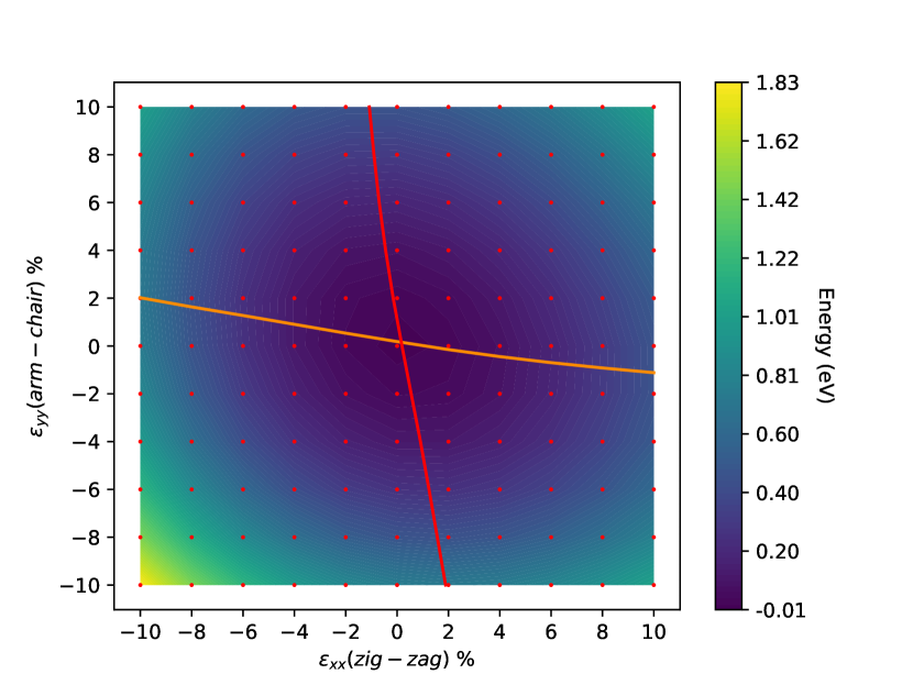
Figure 1: Plot of the total energy of graphene against the values of $\varepsilon_{xx/yy}$. The dark orange (red) curve represents the value of the $\varepsilon_{yy}$ ($\varepsilon_{xx}$) strain that minimizes the energy of the system given the constraint $\varepsilon_{xx}(\varepsilon_{yy})=\mbox{const}$. The red dots represent the sampled combinations of $\epsilon_{xx/yy}$ values used to compute the total energy of the system.

III Ab initio results

III.1 Strain dependence of the WF and extraction of the deformation potential for graphene

The strain dependence of the work function in graphene is computed using the PBE functional, since, as shown in Fig. 2 for biaxial strain, the value of the WF turns out to be quite sensitive to the choice of the XC functional but its slope is not. This implies that physical quantities like the deformation potential, which is basically related to the first derivative of these curves, can be assessed with less ambiguity.

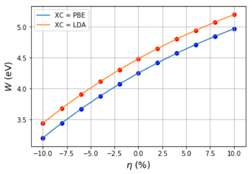
Figure 2: Dependence of the work function of graphene on the values of biaxial strain for the PBE and LDA XC functionals.

The WF dependence of graphene on biaxial and uniaxial strains is computed for values of strain in the range from $-16\%$ to $+16\%$. For the uniaxial cases, deformation in both zigzag and armchair directions is investigated taking into account the associated PR. Results are reported in the top panel of Fig. 3 and show good agreement with the literature Giovannetti et al. (2008); Choi et al. (2010); Ziegler et al. (2011); Batrakov et al. (2019); Legesse et al. (2017); Yang et al. (2017); Postorino et al. (2020).

We observe that the WF grows as the tensile strain increases. A possible explanation for this trend is based on the fact that, as long as the material is stretched, the interaction among the ions of the lattice decreases. In this way the system approaches the behavior of isolated atoms in the limit of infinite tensile deformation. The ionization potential for the C atom is $11.2\text{\,}\mathrm{e}\mathrm{V}$, a value much higher than the WF of its corresponding two dimensional form at equilibrium, $4.25\text{\,}\mathrm{e}\mathrm{V}$ in PBE ($4.48\text{\,}\mathrm{e}\mathrm{V}$ in LDA). For this reason, it is expected that the WF of graphene, characterized by fully covalent bonds, should grow with increasing uniform tensile deformation.

We also observe that the change rate of the WF depends on the type of strain applied. In particular, uniaxial strains highlight an almost identical behavior between the zigzag and armchair directions, with small differences only for high values of the deformation. For biaxial strain a steeper change rate is observed. This difference is due to the fact that, for a given value of $\eta$, the lattice deformation is larger for biaxial strain since the atoms are uniformly displaced in all directions.

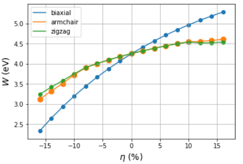
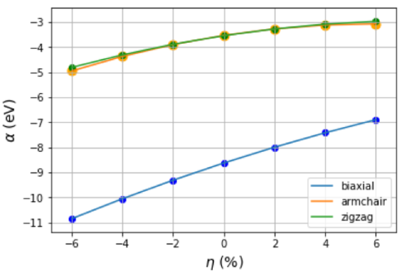
Figure 3: Results for graphene. Top panel: Work function dependence on the biaxial (blue dots), the uniaxial-zigzag (green dots), and the uniaxial-armchair (orange dots) strain from $-16\%$ (compressive) to $+16\%$ (tensile). Bottom panel: Deformation potential $\alpha$ associated with biaxial and uniaxial strains.

Knowing the WF dependence of the strain we extract the deformation potential $\alpha$, defined as

$$\alpha_{s}=-\frac{dW_{s}^{\eta}}{d\eta}.$$ (7)

Here, $W_{s}^{\eta}$ indicates the value of the WF corresponding to a strain of magnitude $\eta$ and the index $s$ takes the values $\mathrm{bi,arm}$ and $\mathrm{zig}$. We emphasize that for the uniaxial armchair and zigzag strains the deformation potential in Eq. (7) is calculated taking into account the PR.

The ab initio estimate of Eq. (7) is evaluated through a polynomial fitting of the WF curves in the top panel of Fig. 3 and by the subsequent computation of the first derivative for each value of strain. This procedure is restricted to a limited range (from $-6\%$ to $+6\%$), since the WF curves become less smooth for higher strain values, and the numerical extraction of the derivative becomes less trivial. Corresponding results, reported in the bottom panel of Fig. 3, show that in graphene the zigzag and armchair deformation potentials are practically identical, and much weaker than the biaxial one, for the reasons discussed above.

III.2 Strain dependence of the WF and extraction of deformation potential for silicene

The same analysis described for graphene is performed also for silicene, using the PBE functional for both tensile and compressive deformations. The optimized equilibrium lattice constant is found to be equal to $3.867\text{\,}\AA$ with a buckling of $0.448\text{\,}\AA$. The WF for zero strain is obtained to be $4.35\text{\,}\mathrm{e}\mathrm{V}$ (a test calculation in LDA gives a value of $4.76\text{\,}\mathrm{e}\mathrm{V}$). Also for silicene, the PR of the system is computed ab initio by employing the same procedure used for graphene (see Fig. 4).

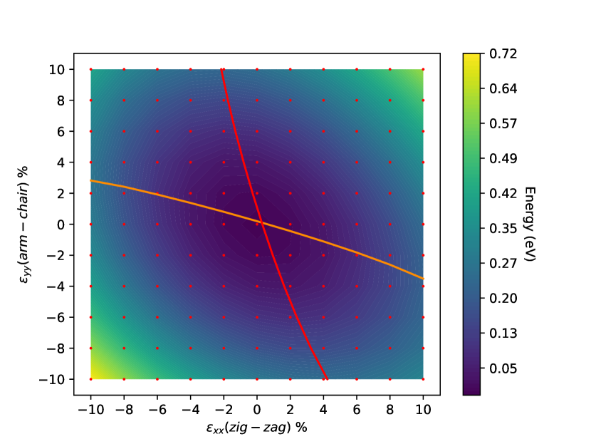
Figure 4: Plot of the total energy of silicene against the values of $\varepsilon_{xx/yy}$. The dark orange (red) curve represents the value of the $\varepsilon_{yy}$ ($\varepsilon_{xx}$) strain that minimizes the energy of the system given the constraint $\varepsilon_{xx}(\varepsilon_{yy})=\mbox{const}$. The red dots represent the sampled combinations of $\epsilon_{xx/yy}$ values used to compute the total energy of the system.

Results are reported in Fig. 5 and show the strain dependence for both the WF and the deformation potential. In particular, the behavior of the WF is presented for values of strain that range from $+16\%$, in the tensile region, down to $-10\%$, in the compressive part. The curves present a smooth behavior only for values of strain limited from $-4\%$ up to $+4\%$. This non-monotonic behavior of the WF is due to the fact that, for high values of strain (compressive or tensile) there is a change in the electronic band structure. In particular, for high tensile strains, an empty band goes down in energy and crosses the Fermi level close to $\Gamma$ [see the inset in Fig. 5]. On the other hand, for high compressive strains, a filled band near $\Gamma$ increases its energy and crosses the Fermi level from below. All these major modifications of the electronic band structure shift the Fermi level away from the Dirac point. This causes a nonregular trend of the work function vs strain in the case of silicene. In graphene, instead, this does not happen (at the considered strain values) because the gap at $\Gamma$ is much larger than the silicene one.

The obtained data show that, analogously to what happens for graphene, the WF increases with increasing stretching. This increasing occurs since in the limit of infinite tensile strain the WF tends towards the atomic ionization potential, $8.1\text{\,}\mathrm{e}\mathrm{V}$ in silicon.

We calculate the deformation potential by extracting the numerical derivative of the WF in the range of -4% up to +4% . A comparison with the results for graphene highlights that the values of the deformation potential obtained for silicene are much smaller in all the considered cases.

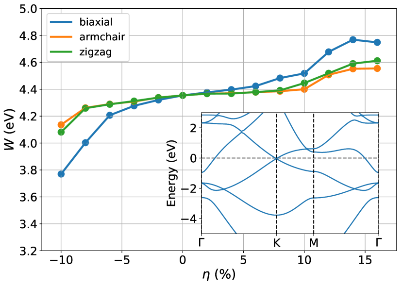
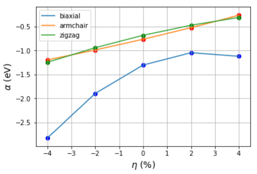
Figure 5: Results for silicene. Top panel: Work function dependence on the biaxial (blue dots), the uniaxial-zigzag (green dots), and the uniaxial-armchair (orange dots) strain. The inset shows the bands structure of the system with a biaxial strain of $12\%$. Bottom panel: Deformation potential $\alpha$ associated with biaxial and uniaxial strains.

IV Deformation potential in the tight-binding strained Hamiltonian

In this section we relate the obtained above results to the parameters of the tight-binding Hamiltonian. The electrons in the valence and conduction bands of graphene and silicene are described by the following Hamiltonian

$$\mathrm{H}=\mathrm{H}_{\mathrm{hop}}+\mathrm{H}_{\mathrm{pot}}.$$ (8)

Here $\mathrm{H}_{\mathrm{hop}}$ is the conventional tight-binding Hamiltonian for $\pi$ orbitals that describes hopping between nearest-neighbors Vozmediano et al. (2010); Amorim et al. (2016); Naumis et al. (2017). We do not write down its explicit form since the corresponding hopping parameters and their strain dependence are not considered in the present work.

The main interest for us represents the potential term

$$\mathrm{H}_{\mathrm{pot}}=\sum_{i,\delta}U^{\phantom{\dagger}}_{\delta i}\hat{c}^{\dagger}_{\delta i}\hat{c}^{\phantom{\dagger}}_{\delta i},$$ (9)

where $i$ run over $N/2$ lattice cells, indices $\delta=A$ and $B$ enumerate the sublattices, operator $\hat{c}_{\delta,i}^{\dagger}$ ($\hat{c}_{\delta,i}$) creates (annihilates) an electron at the corresponding lattice site, the spin index is omitted for brevity, and $U_{\delta i}$ is the on-site deformation-dependent potential. $U_{\delta i}$ consists of the strain-independent part $E_{\mathrm{D}}$, which determines the energy of the Dirac point in unstrained graphene, and the strain-dependent part.

For uniform strain, the potential energy does not depend on the lattice site. Assuming also the linear dependence of the on-site energy on strain, one can rewrite the Hamiltonian (9) as follows:

$$\mathrm{H}_{\mathrm{pot}}=\sum_{i,\delta}(\alpha_{xx}\varepsilon_{xx}+\alpha_{yy}\varepsilon_{yy}+E_{\mathrm{D}})c^{\dagger}_{\delta i}c_{\delta i}.$$ (10)

Here we introduced two deformation potential constants: $\alpha_{xx}$ and $\alpha_{yy}$. The values of these constants are determined from the strain dependence of the WF:

$$\alpha_{xx}=-\left(\frac{\partial W}{\partial\varepsilon_{xx}}\right)_{\varepsilon_{yy}=0},\quad\alpha_{yy}=-\left(\frac{\partial W}{\partial\varepsilon_{yy}}\right)_{\varepsilon_{xx}=0},$$ (11)

where $xx$ and $yy$ correspond to the armchair and zigzag directions, respectively. The range of validity of Eq. (10) follows from the results presented in Figs. 3 and 5 and discussed in Sec. III. For graphene this corresponds to strain values from $-6\%$ to $6\%$, and for silicene this corresponds to strain values from $-4\%$ to $4\%$.

In Sec. III we determined the $\alpha_{s}$ values, which describe the deformation of the samples in the presence of Poisson’s transverse contraction characterized by $\nu_{s}$ with $s=\mathrm{arm}$ and $\mathrm{zig}$. These parameters can be related to each other by taking into account that

$$\begin{split}\frac{dW^{\eta}_{\mathrm{arm}}}{d\eta}&=\frac{\partial W}{\partial\varepsilon_{xx}}-\nu_{\mathrm{arm}}\frac{\partial W}{\partial\varepsilon_{yy}},\\ \frac{dW^{\eta}_{\mathrm{zig}}}{d\eta}&=-\nu_{\mathrm{zig}}\frac{\partial W}{\partial\varepsilon_{xx}}+\frac{\partial W}{\partial\varepsilon_{yy}}.\end{split}$$ (12)

Now we assume that the corresponding derivatives are constants for small values of the strain. Solving the system (12) one obtains

$$\begin{split}\alpha_{xx}&=\frac{\alpha_{\mathrm{arm}}+\nu_{\mathrm{arm}}\alpha_{\mathrm{zig}}}{1-\nu_{\mathrm{arm}}\nu_{\mathrm{zig}}},\\ \alpha_{yy}&=\frac{\alpha_{\mathrm{zig}}+\nu_{\mathrm{zig}}\alpha_{\mathrm{arm}}}{1-\nu_{\mathrm{arm}}\nu_{\mathrm{zig}}}.\end{split}$$ (13)

The values of the constants $\alpha_{s}$, $\alpha_{xx,yy}$ and the PR for the tensile strain for graphene and silicene are provided in Table 1.

​ ​ Graphene ​​	​​ Armchair ​​	​​ Zigzag ​​	​​ Biaxial ​​
$\alpha_{s}$ (eV)	-3.5	-3.5	-8.6
$\nu_{\mathrm{arm,zig}}$	0.14	0.14	–
$\alpha_{xx,yy}$ (eV) for $\nu=0$	-4.1	-4.1	–
​​ Silicene ​​	Armchair	Zigzag	Biaxial
$\alpha_{s}$ (eV)	-0.8	-0.7	-1.3
$\nu_{\mathrm{arm,zig}}$	0.22	0.13	–
$\alpha_{xx,yy}$ (eV) for $\nu=0$	-0.71	-0.49	–

Table 1: The values of deformation potential constants $\alpha_{s}$, with $s=\mathrm{bi,arm,zig}$; $\alpha_{xx,yy}$; and the Poisson’s ratios $\nu_{arm,zig}$ (for the tensile strain) for graphene and silicene, calculated in the vicinity of $\eta=0$.

V Collapse of Landau levels

As mentioned in the Introduction, the energy spectrum of the graphene Dirac fermions in crossed external magnetic and electric fields Lukose et al. (2007); Peres and Castro (2007) is given by Eq. (1), with the corresponding Landau scale shown by Eq. (2). It is easy to see from these equations that, in the case of a constant value of the in-plane electric field $E$, the Landau levels would collapse as the magnetic field reaches the value $B_{c}=E/v_{F}$ from above. Some indications of this effect have been obtained experimentally in Refs. Singh and Deshmukh (2009); Gu et al. (2011).

Interestingly, in Dirac materials the strain can induce the same phenomena. The experimental observation of the Landau levels induced by inhomogeneous strain Levy et al. (2010) is probably the most spectacular effect associated with straintronics Levy et al. (2010). The key point is that the strain-induced change in the hopping energy between neighboring atoms in the Hamiltonian $\mathrm{H}_{\mathrm{hop}}$ can be described by some kind of vector potential $\mathbf{A}_{\mathrm{pm}}$ (see Refs. Vozmediano et al. (2010); Amorim et al. (2016) for a review). For the $x$-axis aligned in the armchair direction Kitt et al. (2012), it reads

$$\mathbf{A}_{\mathrm{pm}}=\frac{\hbar\beta}{2a_{0}}\left(\begin{array}[]{c}2\varepsilon_{xy}\\ \varepsilon_{xx}-\varepsilon_{yy}\\ \end{array}\right),$$ (14)

where $\beta$ is the dimensionless Grüneisen parameter for the lattice deformation and $a_{0}$ is the lattice constant. The generic position-dependent strain tensor $\varepsilon_{ij}$, with $i,j=x,y$, is related to the displacement (5) by the relation $\varepsilon_{ij}=(\partial_{i}u_{j}+\partial_{j}u_{i})/2$.

The vector potential, Eq. (14), generates a pseudomagnetic field $\mathbf{B}_{\mathrm{pm}}=\mathbf{\nabla}\times\mathbf{A}_{\mathrm{pm}}$. It formally resembles a real magnetic field, with the crucial distinction that it is directed oppositely in $\mathbf{K}$ and $\mathbf{K}^{\prime}$ valleys. The sign of the pseudomagnetic field depends on the valley, and, for example, in the $\mathbf{K}$ valley,

$$B_{\mathrm{pm}}=\frac{\hbar\beta}{a_{0}}\left(\frac{1}{2}\partial_{x}(\varepsilon_{xx}-\varepsilon_{yy})-\partial_{y}\varepsilon_{xy}\right),$$ (15)

whereas it has the opposite sign in the $\mathbf{K}^{\prime}$ valley.

Then, the deformation potential part of the Hamiltonian $\mathrm{H}_{\mathrm{pot}}$, Eq. (10), contains the scalar potential $\alpha A_{0}=\alpha(\varepsilon_{xx}+\varepsilon_{yy})$, which has the same sign in both the $\mathbf{K}$ and $\mathbf{K}^{\prime}$ valleys. Accordingly, the deformation potential acts as an electric field per unit charge $E_{i}=-\alpha_{ik}\partial_{k}A_{0}$. Bearing in mind the isotropic graphene (see Table 1), we assume that $\alpha_{xx}=\alpha_{yy}=\alpha$. Yet, since in silicene $\alpha_{xx}\neq\alpha_{yy}$, the results presented below are not directly applicable.

One can see that uniform strain results in the appearance of a constant strain-induced vector potential corresponding to the shift of the $\mathbf{K}$ and $\mathbf{K}^{\prime}$ points, so that the pseudomagnetic field is zero. Since $A_{0}$ is position independent, also an electric field is absent.

On the other hand, creation of the pseudo Landau levels requires a special configuration with inhomogeneous strain. To simplify theoretical modeling, the pseudo Landau levels are very often treated assuming that the deformation is a pure shear, so that $A_{0}=\varepsilon_{xx}+\varepsilon_{yy}=0$, and the corresponding term in the Hamiltonian does not appear. This assumption is rather unphysical, and when the deformation potential is included, new effects are expected. For some strain configurations, the deformation potential acts as an in-plane electric field.

A special strain configuration was considered in Ref. Castro et al. (2017). In our notations it can be written as $\varepsilon_{xx}=2a_{0}Bx/(\beta\hbar)$, $\varepsilon_{yy}=0$, and $\varepsilon_{xy}=0$. It corresponds to the strain-induced vector and scalar potentials $A_{\mathrm{pm}}=(0,Bx)$ and $A_{0}=2a_{0}Bx/(\beta\hbar)$, respectively. Evidently, they generate crossed constant pseudomagnetic and electric fields of the magnitudes $B$ and $E_{x}=-2a_{0}\alpha B/(\beta\hbar)$. Then, the condition of the Landau level collapse acquires the form $|\alpha|\gtrsim v_{F}\beta\hbar/(2a_{0})$ Lukose et al. (2007); Castro et al. (2017). One can see that in this case the condition for the collapse depends on the material constants $\alpha$, $\beta$, and $v_{F}$, which cannot be tuned easily.

Here we propose a different experimental setup with a special strain configuration that generates only the electric field, while the pseudomagnetic field is absent. Then, applying a real magnetic field, one should be able to realize the Landau level collapse. In fact, we obtain a pseudomagnetic field of $B_{\mathrm{pm}}=0$ when in Eq. (14) the components of the pseudo vector potential are constants, i.e., $A_{x}=C_{1}$ and $A_{x}=C_{2}$. Then it is easy to see that this is possible when the components of the displacement vector $u_{x,y}(x,y)$ satisfy the two-dimensional Laplace equations:

$$\begin{split}\frac{\partial^{2}u_{x}}{\partial x^{2}}+\frac{\partial^{2}u_{x}}{\partial y^{2}}&=0,\\ \frac{\partial^{2}u_{y}}{\partial x^{2}}+\frac{\partial^{2}u_{y}}{\partial y^{2}}&=0.\end{split}$$ (16)

Any harmonic function satisfies Eq. (16), so one can consider the simplest nontrivial example:

$$\begin{split}u_{x}(x,y)&=d(x^{2}-y^{2})+h_{1}x+h_{2}y,\\ u_{y}(x,y)&=2dxy+h_{3}x+h_{4}y.\end{split}$$ (17)

Here $d$ is a constant that has the dimension of an inverse length, while $h_{1,2,3,4}$ are the dimensionless constants that describe the uniform strain.

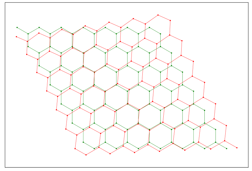
Figure 6: Example of a nonuniform strained lattice (red) built applying Eq. (17) to ideal graphene (green). We used $da_{0}=0.01$ and $h_{1,2,3,4}=0.1$.

This strain configuration, shown in Fig. 6, generates the following potentials:

$$\begin{split}A_{x}=&\frac{\beta}{2a_{0}}(h_{2}+h_{3}),\qquad A_{y}=\frac{\beta}{2a_{0}}(h_{1}-h_{4}),\\ &A_{0}=4dx+h_{1}+h_{4}.\end{split}$$ (18)

One can see that this potential corresponds to $B_{\mathrm{pm}}=0$ and a constant electric field $E_{x}=-4\alpha d/e$, where we explicitly included the electric charge $e$. The constant term $\alpha(h_{1}+h_{4})$ in $\mathrm{H}_{\mathrm{pot}}$ corresponds to the uniform strain considered in the previous sections.

When a constant external magnetic field is applied in addition to the strain induced electric field, the condition of the Landau levels collapse $E=v_{F}B_{c}$ Lukose et al. (2007) acquires the following form

$$B_{c}=\frac{4(da_{0})|\alpha|}{ea_{0}v_{F}}.$$ (19)

Thus, as the magnetic field decreases to this critical value $B_{c}$, the collapse occurs. This is illustrated in the top panel of Fig. 7, where the energies of strain-affected Landau levels $E_{n}-E_{0}$ in the units of the Landau scale $\omega_{L}$ are shown for the two values of $B/B_{c}$. They tend to the energy of the lowest Landau level as $B$ approaches $B_{c}$.

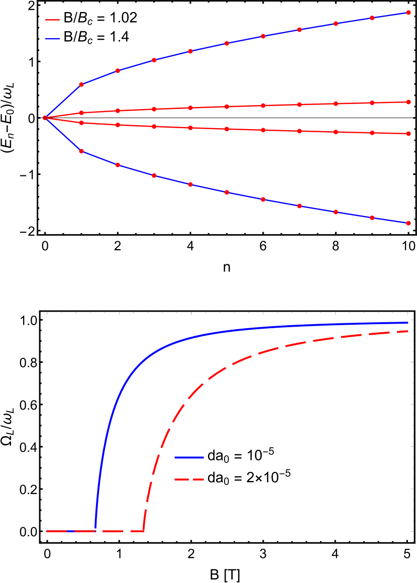
Figure 7: Top panel: the Landau level energies $(E_{n}-E_{0})/\omega_{L}$ for $B/B_{c}=1.4$ and $1.02$. Bottom panel: the dependence of the Landau scale $\Omega_{L}/\omega_{l}$ on the magnetic field $B$ for $da_{0}=10^{-5}$ and $2\times 10^{-5}$.

Taking into account that $$1\text{\,}\mathrm{T}$=$\text{\,}\mathrm{V}\cdot\mathrm{s}\mathrm{/}\mathrm{m}^{2}$$ and using the value of the Fermi velocity $v_{F}=$1\text{\times}{10}^{6}\text{\,}\mathrm{m}\mathrm{/}\mathrm{s}$$ and $a_{0}=$2.46\text{\,}~{}\AA$$, one obtains the following estimate:

$$B_{c}=$1.63\text{\times}{10}^{4}\text{\,}\mathrm{(}$da_{0})|\alpha|,$$ (20)

where $B_{c}$ is expressed in Tesla, while $\alpha$ is measured in eV.

Assuming a value of $da_{0}=10^{-5}$, one finds that the Landau levels collapse for graphene (see Table 1) would occur at $B_{c}=$0.67\text{\,}\mathrm{T}$$. Although for silicene the value of the critical field is expected to be dependent on the direction of the electrical field, one can make a rough estimate of $B_{c}$ using Eq. (19). Assuming a value ща $|\alpha|=0.6$ eV given by the average of $\alpha_{xx}$ and $\alpha_{yy}$, it gives the critical field $B_{c}=$0.19\text{\,}\mathrm{T}$$. Here we took $v_{F}=$0.5\text{\times}{10}^{6}\text{\,}\mathrm{m}\mathrm{/}\mathrm{s}$$ and the same parameter $d$ as used for graphene.

The dependence of the Landau scale $\Omega_{L}$ of graphene, for two values of the dimensionless parameter $da_{0}$ is presented in the bottom panel of Fig. 7. This example shows that the measurements of the critical field $B_{c}$ can be used to extract the value of $da_{0}$ characterizing the specific of the deformation. The estimates of $B_{c}$ confirm that the experiment, where the electric field is generated by the non-uniform strain and an external real magnetic field $B$ is tuned to its critical value, can be implemented in practice.

VI Conclusions

In this work we show by ab initio calculations how the WFs of graphene and silicene depends on uniform compressive and tensile strains. For small deformations the dependence is linear and corresponding values of the deformation potential parameters are provided in Table 1. In accordance with both the experiment He et al. (2015) and the ab initio results the WFs of graphene and silicene increase under the tensile strain. For small values of strain the armchair and zigzag deformation potentials turn out to be practically identical and approximately correspond to one half of the deformation potential associated with biaxial strain.

It has to be noted that strain tuning of the WFs of different materials has been a topic of research for a long time. As an example we refer to the experiment In Ref. Li and Li (2004) that shows the opposite strain dependence of the WFs in Cu and Al, viz., in the elastic range, tensile strain results in the decrease of the WF. The corresponding ab initio calculation that agreed with the experiment was presented in Ref. Pogosov and Babich (2008). Thus one of the questions for the future is to address how the corresponding strain dependence of the WF is material dependent.

Finally, we propose the experimental setup with a special strain configuration that generates only an electric field, whereas the pseudomagnetic field is absent. In this case, in order to obtain the Landau level staircase, an external magnetic field should be applied. Such a setup allows one to explore the phenomenon of the Landau levels collapse more easily, since the strain-induced electric field and the magnetic field can be controlled independently.

References

- Lukose et al. (2007) V. Lukose, R. Shankar, and G. Baskaran, Phys. Rev. Lett. 98, 116802 (2007).
- Peres and Castro (2007) N. M. R. Peres and E. V. Castro, Journal of Physics: Condensed Matter 19, 406231 (2007).
- Vozmediano et al. (2010) M. Vozmediano, M. Katsnelson, and F. Guinea, Physics Reports 496, 109 (2010).
- Amorim et al. (2016) B. Amorim, A. Cortijo, F. de Juan, A. Grushin, F. Guinea, A. Gutiérrez-Rubio, H. Ochoa, V. Parente, R. Roldán, P. San-Jose, J. Schiefele, M. Sturla, and M. Vozmediano, Physics Reports 617, 1 (2016).
- Naumis et al. (2017) G. G. Naumis, S. Barraza-Lopez, M. Oliva-Leyva, and H. Terrones, Reports on Progress in Physics 80, 096501 (2017).
- Cahen and Kahn (2003) D. Cahen and A. Kahn, Advanced Materials 15, 271 (2003).
- Yu et al. (2009) Y.-J. Yu, Y. Zhao, S. Ryu, L. E. Brus, K. S. Kim, and P. Kim, Nano Letters 9, 3430 (2009).
- Yan et al. (2012) R. Yan, Q. Zhang, W. Li, I. Calizo, T. Shen, C. A. Richter, A. R. Hight-Walker, X. Liang, A. Seabaugh, D. Jena, H. Grace Xing, D. J. Gundlach, and N. V. Nguyen, Applied Physics Letters 101, 022105 (2012), https://doi.org/10.1063/1.4734955 .
- Xu et al. (2012) K. Xu, C. Zeng, Q. Zhang, R. Yan, P. Ye, K. Wang, A. C. Seabaugh, H. G. Xing, J. S. Suehle, C. A. Richter, D. J. Gundlach, and N. V. Nguyen, Nano Letters 13, 131 (2012).
- Samaddar et al. (2016) S. Samaddar, J. Coraux, S. C. Martin, B. Grévin, H. Courtois, and C. B. Winkelmann, Nanoscale 8, 15162 (2016).
- He et al. (2015) X. He, N. Tang, X. Sun, L. Gan, F. Ke, T. Wang, F. Xu, X. Wang, X. Yang, W. Ge, and B. Shen, Applied Physics Letters 106, 043106 (2015).
- Volodin et al. (2017) A. Volodin, C. Van Haesendonck, O. Leenaerts, B. Partoens, and F. M. Peeters, Applied Physics Letters 110, 193101 (2017), https://doi.org/10.1063/1.4982931 .
- Castro et al. (2017) E. V. Castro, M. A. Cazalilla, and M. A. H. Vozmediano, Phys. Rev. B 96, 241405 (2017).
- Guinea et al. (2010) F. Guinea, A. K. Geim, M. I. Katsnelson, and K. S. Novoselov, Phys. Rev. B 81, 035408 (2010).
- Choi et al. (2010) S.-M. Choi, S.-H. Jhi, and Y.-W. Son, Phys. Rev. B 81, 081407 (2010).
- Lanzillo et al. (2015) N. A. Lanzillo, A. J. Simbeck, and S. K. Nayak, Journal of Physics: Condensed Matter 27, 175501 (2015).
- Giannozzi et al. (2009) P. Giannozzi, S. Baroni, N. Bonini, M. Calandra, R. Car, C. Cavazzoni, D. Ceresoli, G. L. Chiarotti, M. Cococcioni, I. Dabo, et al., Journal of Physics: Condensed matter 21, 395502 (2009).
- Giannozzi et al. (2017) P. Giannozzi, O. Andreussi, T. Brumme, O. Bunau, M. B. Nardelli, M. Calandra, R. Car, C. Cavazzoni, D. Ceresoli, M. Cococcioni, et al., Journal of Physics: Condensed Matter 29, 465901 (2017).
- Kohn and Sham (1965) W. Kohn and L. J. Sham, Phys. Rev. 140, A1133 (1965).
- Perdew and Zunger (1981) J. P. Perdew and A. Zunger, Physical Review B 23, 5048 (1981).
- Perdew et al. (1996) J. P. Perdew, K. Burke, and M. Ernzerhof, Physical Review Letters 77, 3865 (1996).
- Giovannetti et al. (2008) G. Giovannetti, P. A. Khomyakov, G. Brocks, V. M. Karpan, J. van den Brink, and P. J. Kelly, Phys. Rev. Lett. 101, 026803 (2008).
- Ziegler et al. (2011) D. Ziegler, P. Gava, J. Güttinger, F. Molitor, L. Wirtz, M. Lazzeri, A. M. Saitta, A. Stemmer, F. Mauri, and C. Stampfer, Phys. Rev. B 83, 235434 (2011).
- Batrakov et al. (2019) K. G. Batrakov, N. I. Volynets, A. G. Paddubskaya, P. P. Kuzhir, M. S. Prete, O. Pulci, E. Ivanov, R. Kotsilkova, T. Kaplas, and Y. Svirko, physica status solidi (b) 256, 1800683 (2019).
- Legesse et al. (2017) M. Legesse, F. E. Mellouhi, E. T. Bentria, M. E. Madjet, T. S. Fisher, S. Kais, and F. H. Alharbi, Applied Surface Science 394, 98 (2017).
- Yang et al. (2017) N. Yang, D. Yang, L. Chen, D. Liu, M. Cai, and X. Fan, Nanoscale Research Letters 12, 642 (2017).
- Postorino et al. (2020) S. Postorino, D. Grassano, M. D’Alessandro, A. Pianetti, O. Pulci, and M. Palummo, Nanomaterials and Nanotechnology 10 (2020), 10.1177/1847980420902569.
- Singh and Deshmukh (2009) V. Singh and M. M. Deshmukh, Phys. Rev. B 80, 081404 (2009).
- Gu et al. (2011) N. Gu, M. Rudner, A. Young, P. Kim, and L. Levitov, Phys. Rev. Lett. 106, 066601 (2011).
- Levy et al. (2010) N. Levy, S. A. Burke, K. L. Meaker, M. Panlasigui, A. Zettl, F. Guinea, A. H. C. Neto, and M. F. Crommie, Science 329, 544 (2010).
- Kitt et al. (2012) A. L. Kitt, V. M. Pereira, A. K. Swan, and B. B. Goldberg, Phys. Rev. B 85, 115432 (2012).
- Li and Li (2004) W. Li and D. Y. Li, Philosophical Magazine 84, 3717 (2004).
- Pogosov and Babich (2008) V. V. Pogosov and A. V. Babich, Technical Physics 53, 1074 (2008).