Distribution of missing differences in diffsets

Abstract.

Lazarev, Miller and O'Bryant [LMO] investigated the distribution of $|S+S|$ for $S$ chosen uniformly at random from $\{0,1,\dots,n-1\}$, and proved the existence of a divot at missing 7 sums (the probability of missing exactly 7 sums is less than missing 6 or missing 8 sums). We study related questions for $|S-S|$, and shows some divots from one end of the probability distribution, $P(|S-S|=k)$, as well as a peak at $k=4$ from the other end, $P(2n-1-|S-S|=k)$. A corollary of our results is an asymptotic bound for the number of complete rulers of length $n$.

1. Introduction

1.1. Background

Let $S$ be a typical subset of

$$[n]\ :=\ \{0,1,\dots,n-1\};$$ (1.1)

in other words, we choose $S$ uniformly at random, or equivalently each integer in $[n]$ is independently chosen to be in $S$ with probability $1/2$. Define

$$S+S\ :=\ \{x+y:x,y\in S\}{\rm\ and\ }S-S:=\{x-y:x,y\in S\}.$$ (1.2)

We refer to these as the sumset and the diffset of $S$, and we denote the cardinality of a set $A$ by $|A|$.

The sizes of the sumset and the diffset have been compared extensively. As addition is commutative and subtraction is not, it was conjectured that as $n\to\infty$ almost all sets $S$ should be difference dominated: $|S-S|>|S+S|$. Thus while sum-dominant sets were known to exist, and constructions for infinite families were given, they were thought to be rare. This conjecture turns out to be false; Martin and O'Bryant [MO] proved that for a small but positive proportion of all subsets of $[n]$, the sumset has a larger cardinality than the diffset. This result holds if instead of choosing each element with probability 1/2 we instead choose with a fixed probability $p>0$; however, if $p$ is allowed to decay to zero with $n$ then Hegarty and Miller [HM] proved almost all sets are difference dominated. For these and related results see [AMMS, BELM, CLMS, CMMXZ, DKMMW, DKMMWW, He, HLM, ILMZ, MA, MOS, MP, MS, MV, MXZ, Na1, Na2, Ru1, Ru2, Ru3, Zh1, Zh2].

The distribution of $|S+S|$ has also been studied. When $S$ is chosen uniformly at randomly from $[n]$, Lazarev, Miller and O'Bryant [LMO] proved an unusual ``divot'' occurs in the limiting probability distribution of $|S+S|$ (the existence of the limiting distribution was shown by Zhao [Zh2]). In particular, the limiting probability of missing 7 sums is less than that of missing 6 (or 8):

$$\lim\limits_{n\to\infty}P(2n-1-|S+S|=7)<\lim\limits_{n\to\infty}P(2n-1-|S+S|=6)<\lim\limits_{n\to\infty}P(2n-1-|S+S|=8).$$ (1.3)

Further, [LMO] gave rigorous bounds for $\lim\limits_{n\to\infty}P(2n-1-|S+S|=k)$ for $0\leq k<32$, which imply that there are no more divots until $k=27$. It is unknown whether there could be more divots later. Figure 1 of their paper is reproduced here with permission as Figure 1.

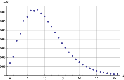
Figure 1. Experimental values of $m(k)$, the probability $S+S$ is missing exactly $k$ sum, when each $m\in[n]$ is in $S$ with probability $1/2$. The vertical bars depict the values allowed by the most rigorous bounds in [LMO]. In most cases, the allowed interval is smaller than the dot indicating the experimental value. The data comes from generating $2^{28}$ sets uniformly forced to contain 0 from $[0,256)$.

However, the probability distribution of $|S-S|$, the size of the diffset, has not been extensively investigated. One reason for the success in $|S+S|$ and the lack of progress for $|S-S|$ is that the sumset is significantly easier to exhaustively investigate. For many sets, their properties can be determined by decomposing $S$ as $L\cup M\cup R$, where $L$ and $R$ are respectively the left and right fringe elements and $M$ is the middle; typically $L$ and $R$ are of bounded size independent of $n$, so most elements in $S$ are in $M$. As there are many ways to write a number as a sum or difference of elements, most elements in $[n]+[n]$ or $[n]-[n]$ are realized, especially since a typical $S$ has on the order of $n/2$ elements and thus generates on the order of $n^{2}/2$ pairs. The difference is for the fringe elements, where there are fewer representations and thus a greater chance of an element not being obtained. For sumsets the left and right fringes do not interact, with the left fringe $L+L$ and the right $R+R$; this is not the case for the diffset, where the fringes are $L-R$ and its negative $R-L$. As a result, to determine whether an extremal element is in $S+S$, only one fringe matters while for $S-S$, both ends must be considered. The computational complexity is hence squared, which makes the diffset distribution significantly harder to exhaustively investigate.

Below we focus on the probability distribution of $|S-S|$.

1.2. Distribution of $|S-S|$ when $n=35$

We display the probability distribution when $n=35$ in Figure 2. We exhaustively listed every subset of $[n]$ and recorded the corresponding $|S-S|$. The probability distribution is exactly the frequencies divided by $2^{35}$.

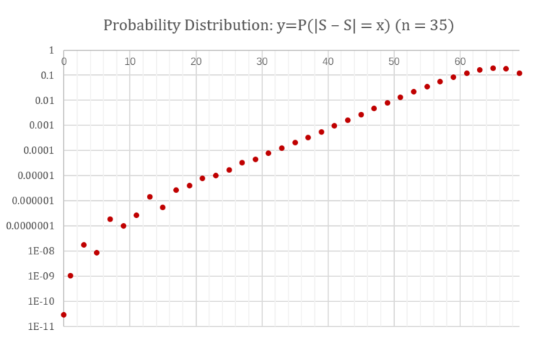
Figure 2. Probability distribution of $P(|S-S|=x)$ when $n=35$.

We make three observations from Figure 2.

• $|S-S|$ is either 0 or odd.

• There are divots at having 5, 9 and 15 differences. That is,

  $$P(|S-S|=3) \ >\ P(|S-S|=5)\ <\ P(|S-S|=7),$$

  $$P(|S-S|=7) \ >\ P(|S-S|=9)\ <\ P(|S-S|=11),{\rm\ and\ }$$

  $$P(|S-S|=13) \ >\ P(|S-S|=15)\ <\ P(|S-S|=17).$$ (1.4)

• There is a peak at ``missing 4'' differences. That is,

  $$\forall k\neq 4,P(2n-1-|S-S|=4)\ >\ P(2n-1-|S-S|=k)$$ (1.5)

  (thus when $n=35$, this is saying $|S-S|=65$ is the most likely cardinality of the diffset).

These observations seem to continue to hold for larger $n$, though our investigations are no longer exhaustive but instead are random samples from the space.

The first observation is trivial after realizing that if $m\in S-S$ then $-m\in S-S$.

For conciseness, let

$$P_{n}^{\text{H}}(k)\ :=\ P(|S-S|=k),\ \ \ P_{n}^{\text{M}}(k)\ :=\ P(2n-1-|S-S|=k).$$ (1.6)

Here, H means having differences whereas M means missing. They are two complementary perspectives.

1.3. Main results

We prove that Observations 2 and 3 are true for sufficiently large $n$.

Theorem 1.1.

Observation 2 is true for $n\geq 12$. That is, $\forall n\geq 12,$

$$P_{n}^{\text{H}}(3)\ >\ P_{n}^{\text{H}}(5)\ <\ P_{n}^{\text{H}}(7),$$

$$P_{n}^{\text{H}}(7)\ >\ P_{n}^{\text{H}}(9)\ <\ P_{n}^{\text{H}}(11),$$

$${\rm\ and\ } P_{n}^{\text{H}}(13)\ >\ P_{n}^{\text{H}}(15)\ <\ P_{n}^{\text{H}}(17).$$ (1.7)

(Note that when $n=11$, Observation 2 fails because $P_{n}^{\text{H}}(13)=269<275=P_{n}^{\text{H}}(15)$.)

Theorem 1.2.

Observation 3 is true for sufficiently large $n$. That is,

$$\exists N:\forall n\geq N,\forall k\neq 4:\ P_{n}^{\text{M}}(4)\ >\ P_{n}^{\text{M}}(k).$$ (1.8)

(Note that when $n=14$, Observation 3 fails because $P_{n}^{\text{M}}(4)=P_{n}^{\text{M}}(2)$. We don't know if this will ever happen again for larger $n$.)

Similar to Theorem 1.9 in [LMO], we have the following result, which is used to prove Theorem 1.2.

Theorem 1.3.

The limiting probability distribution of missing differences,
$\ell(k):=\lim\limits_{n\to\infty}P_{n}^{\text{M}}(k)$, is well-defined, positive on (and only on) even $k$'s, adds up to $1$, and satisfies

$$\ell(10)\ <\ \ell(8)\ <\ \ell(0)\ <\ \ell(6)\ <\ \ell(2)\ <\ \ell(4).$$ (1.9)

Rigorous bounds for $\ell(k)$ are given in Theorem 3.20. As a corollary, we provide an asymptotic bound for the OEIS sequence A103295, which counts the number of complete rulers.

Theorem 1.4.

The OEIS sequence A103295 satisfies $a_{n}\sim c\cdot 2^{n}$, where $0.2433<c<0.2451$.

2. Results about having (few) differences

We give a few straightforward results on having few differences.

Definition 2.1.

A sequence $Q$ has a divot at $i$ if $Q_{i}$ is smaller than the nearest non-zero neighbor on each side of the sequence.

Note in the above definition we require the neighbors to be non-zero; this is important as the cardinalities of the number of missing differences is always even.

Proposition 2.2.

For all $n\geq 4$, $P_{n}^{\text{H}}$ has a divot at 5: $P_{n}^{\text{H}}(3)>P_{n}^{\text{H}}(5)<P_{n}^{\text{H}}(7)$.

Proof.

We have the following characterizations, where we abbreviate a set $S$ is an arithmetic progression by writing $S$ is an AP.

• $|S-S|=3\Longleftrightarrow|S|=2$.

• $|S-S|=5\Longleftrightarrow|S|=3{\rm\ and\ }S\text{ is an AP (e.g., }\{3,8,13\}\text{)}$.

• $|S-S|=7\Longleftrightarrow|S|=3{\rm\ and\ }S\text{ is not an AP,}{\rm\ or\ }|S|=4{\rm\ and\ }S\text{ is an AP}$.

Thus, by counting arithmetic progressions, the following equations hold:

$$2^{n}P_{n}^{\text{H}}(3) \ =\ {n\choose 2}$$

$$2^{n}P_{n}^{\text{H}}(5) \ =\ {\lfloor\frac{n}{2}\rfloor\choose 2}+{\lfloor\frac{n+1}{2}\rfloor\choose 2}$$

$$2^{n}P_{n}^{\text{H}}(7) \ =\ {n\choose 3}-2^{n}P_{n}^{\text{H}}(5)+\sum_{i=0}^{2}{\lfloor\frac{n+i}{3}\rfloor\choose 2}.$$ (2.1)

When $n\geq 4$, we have

$$P_{n}^{\text{H}}(3)\ >\ P_{n}^{\text{H}}(5)\ \leq\ \frac{{n\choose 3}}{2^{n}}-P_{n}^{\text{H}}(5)\ <\ P_{n}^{\text{H}}(7).$$ (2.2)

∎

In view of the proof, for any $k$ we see that $P_{n}^{\text{H}}(k)$ can be written in a closed form in terms of $n$. Straightforward analysis shows the following.

Proposition 2.3.

For all $n\geq 7$, $P_{n}^{\text{H}}$ has a divot at 9.

Proposition 2.4.

For all $n\geq 12$, $P_{n}^{\text{H}}$ has a divot at 15.

The above allows us to conclude Theorem 1.1. $\Box$

3. Results about missing (few) differences

3.1. Intuitively measuring the limiting probabilities

We show that the limiting probability of having $k$ differences, and that of missing $k$ differences, exist. The latter (Claim 3.2) is a special case of Theorem 1.3 in [Zh2], but as some parts of this argument will be used later, we provide details.

Claim 3.1.

For all $k\geq 0$, $\lim\limits_{n\to\infty}P_{n}^{\text{H}}(k)=0$.

Proof.

The claim follows immediately by noting $P(|S-S|=k)\leq P(|S|\leq k)\to 0$. ∎

Claim 3.2.

For all $k\geq 0$, $\lim\limits_{n\to\infty}P_{n}^{\text{M}}(k)$ exists and $\sum_{i=0}^{\infty}\lim\limits_{n\to\infty}P_{n}^{\text{M}}(i)=1$.

Proof.

Recall Observation 1: when $k$ is odd, for all $n\neq\frac{k+1}{2}$ we have $P_{n}^{\text{M}}(k)=0$. We are interested in evens.

$\forall k\geq 0,\forall m>k,\forall\epsilon>0,\forall n>2m,\forall S\subseteq[n],$ if $\{0,\dots,n-m-1\}\subseteq S-S$, then

$$|(S-S)\cap\{n-m,\dots,n-1\}|\ =\ m-k \ \Longleftrightarrow\ |(S-S)\cap\{0,\dots,n-1\}|\ =\ n-k$$

$$\ \Longleftrightarrow\ |S-S|\ =\ 2n-1-2k.$$ (3.1)

Thus

$$\left|P_{n}^{\text{M}}(2k)-P\left(\left|\left(S-S\right)\cap\{n-m,\dots,n-1\}\right|=m-k\right)\right|$$

$$\ \leq\ P(\{0,\dots,n-m-1\}\subsetneq S-S).$$ (3.2)

The main term is constant with respect to $n$:

$$P\left(|(S-S)\cap\{n-m,\dots,n-1\}|=m-k\right)$$

$$=\ \ {} P\left(\left|\left(\left(S\cap\{n-m,\dots,n-1\}\right)-\left(S\cap\{0,\dots,m-1\}\right)\right)\cap\{n-m,\dots,n-1\}\right|=m-k\right)$$

$$=\ \ {} P_{S_{1}\subseteq[n]\setminus(n-m),S_{2}\subseteq[m]}\left(\left|\left(S_{1}-S_{2}\right)\cap\{n-m,\dots,n-1\}\right|=m-k\right)$$

$$=\ \ {} P_{S\subseteq[2m]}\left(\left|\left(S-S\right)\cap\{m,\dots,2m-1\}\right|=m-k\right)$$

$$=:\ {} f_{k}(m).$$ (3.3)

By Lemma 11 in [MO],

$$P(\{0,\dots,n-m-1\}\subsetneq S-S) \ \leq\ \sum_{i=0}^{n-m-1}P(i\notin S-S)$$

$$\ \leq\ \sum_{i=0}^{\lfloor\frac{n}{2}\rfloor-1}\left(\frac{3}{4}\right)^{\frac{n}{3}}+\sum_{i=\lfloor\frac{n}{2}\rfloor}^{n-m-1}\left(\frac{3}{4}\right)^{n-i}$$

$$\ <\ \left(\frac{3}{4}\right)^{\frac{n}{3}}\cdot\frac{n}{2}+\left(\frac{3}{4}\right)^{m+1}\cdot 4$$

$$\ <\ \epsilon+4\left(\frac{3}{4}\right)^{m+1}\text{ for sufficiently large }n.$$ (3.4)

For sufficiently large $n$,

$$\left|P_{n}^{\text{M}}(2k)-f_{k}(m)\right|\ <\ \epsilon+4\left(\frac{3}{4}\right)^{m+1}.$$ (3.5)

By the arbitrariness of $m{\rm\ and\ }\epsilon$, $\{P_{n}^{\text{M}}(2k)\}_{n}$ is Cauchy and so converges. The rest of the claim follows from non-negativity of the limits and the fact $\sum_{i=0}^{2n-1}P_{n}^{\text{M}}(i)=1$. ∎

Remark 3.3.

Note $m>k$ is not needed, and since the bounded error, $\epsilon+4\left(\frac{3}{4}\right)^{m+1}$, is irrelevant to $k$, the convergence is uniform.

Definition 3.4.

Let $\ell(k):=\lim\limits_{n\to\infty}P_{n}^{\text{M}}(k)$.

Lemma 3.5.

For all $k\geq 0$, we have $\ell(2k+2)\ \geq\ \ell(2k)/2$.

Proof.

We have

$$P_{n}^{\text{M}}(2k+2)$$

$$\ =\ P(|S-S|=2n-1-2(k+1))$$

$$\ \geq\ P(n-1\notin S\ \land\ |(S-S)\cap\{-n+2,\dots,n-2\}|=2n-1-2(k+1))$$

$$\ =\ P(n-1\notin S)\cdot P_{S\subseteq[n-1]}(|S-S|=2(n-1)-1-2k)$$

$$\ =\ \frac{1}{2}P_{n-1}^{\text{M}}(2k).$$ (3.6)

Note the left and right hand sides converge to $\ell(2k+2)$ and $\ell(2k)/2$ respectively. ∎

Corollary 3.6.

For all $k\geq 0$, $\lim\limits_{n\to\infty}P_{n}^{\text{M}}(2k)>0$.

Compared with the distribution of having-differences (Claim 3.1), this shows that the direction we view matters. We see non-zero limits at this end.

Remark 3.7.

By Remark A.1,

$$P_{36}^{\text{M}}(0)\ =\ {} \frac{8342197304}{2^{36}} \ \approx\ 0.1214,$$

$$P_{36}^{\text{M}}(2)\ =\ {} \frac{12668987317}{2^{36}} \ \approx\ 0.1843,$$

$$P_{36}^{\text{M}}(4)\ =\ {} \frac{12894355828}{2^{36}} \ \approx\ 0.1876,$$

$$P_{36}^{\text{M}}(6)\ =\ {} \frac{10879185718}{2^{36}} \ \approx\ 0.1583,$$

$$P_{36}^{\text{M}}(8)\ =\ {} \frac{8208838614}{2^{36}} \ \approx\ 0.1195.$$ (3.7)

This gives us a sensible (but not rigorous) estimate of $\ell(k)$.

We do have a rigorous bound of $\ell(k)$, in view of the proof of Claim 3.2.

Proposition 3.8.

For all $m>k$, $\left|\ell(2k)-f_{k}(m)\right|\leq 4(\frac{3}{4})^{m+1}$.

Proof.

Replace $P_{n}^{\text{M}}(2k)$ by $\ell(2k)$ in equation (3.5). ∎

One would like to use this fact to prove Theorem 1.3, since $f_{k}(m)$ is finitely computable. Unfortunately this quickly becomes unrealistic because it takes $4^{m}m^{2}$ computations to exhaustively determine $f_{k}(m)$, and to reduce the uncertainty to $(0.1876-0.1843)/2$ we should have $m\geq 27$. In 2019, it took our laptop around 5 minutes to run $m=17$ with this method, and thus it would need around 25.2 years to computationally verify the theorem. We thus need a better approach, which we describe below.

3.2. Using Conditional Probabilities

Lemma 3.9.

The conditional probability of $k\not\in S-S$, given that $0,n-1\in S$, is bounded by the following:

$$P\left(k\notin S-S\text{ \big{|} }0,n-1\in S\right)\ \begin{cases}\ =\ 0&k=n-1\\ \ =\ \frac{4}{9}\cdot\left(\frac{3}{4}\right)^{n-k}&\frac{n}{2}\leq k<n-1\\ \ \leq\ \frac{4}{9}\cdot\left(\frac{3}{4}\right)^{\frac{n}{3}}&0\leq k<\frac{n}{2}.\end{cases}$$ (3.8)

Proof.

For all $k<n$ let $D:=\left\{\{a,b\}:a,b\in[n],|a-b|=k\right\}$. We say $D^{\prime}\subseteq D$ is mutually disjoint if $\forall p_{1},p_{2}\in D^{\prime}$, $p_{1}\cap p_{2}=\emptyset$. If $D^{\prime}\subseteq D$ is mutually disjoint and $0,n-1\in\bigcup D^{\prime}$ (the union is over all the pairs in $D^{\prime}$), then

$$P\left(k\notin S-S\text{ \big{|} }0,n-1\in S\right) \ =\ P\left(D\cap\mathcal{P}(S)=\emptyset\text{ \big{|} }0,n-1\in S\right)$$

$$\ \leq\ P\left(D^{\prime}\cap\mathcal{P}(S)=\emptyset\text{ \big{|} }0,n-1\in S\right)$$

$$\ =\ \prod_{p\in D^{\prime}}{\left(1-2^{-|p\setminus\{0,n-1\}|}\right)}$$

$$\ =\ \begin{cases}0&k=n-1\\ \frac{4}{9}\cdot\left(\frac{3}{4}\right)^{|D^{\prime}|}&0\leq k<n-1.\end{cases}$$ (3.9)

When $2k>n-1$, $D$ is already mutually disjoint and has size $n-k$; otherwise, we can find a mutually disjoint $D^{\prime}$ with $|D^{\prime}|\geq n/3$, and let $0,n-1\in\bigcup D^{\prime}$ without loss of generality. We hence conclude the lemma.∎

The conditional probability distribution requiring $0,n-1\in S$ is compared with the usual probability distribution without such restriction. We define similar notions to $P_{n}^{\text{M}},f_{k}$.

Definition 3.10.

Let

$$Q_{n}^{\text{M}}(k) \ :=\ P\left(|S-S|=2n-1-k\text{ \big{|} }0,n-1\in S\right);$$

$$g_{k}(m) \ :=\ P_{S\subseteq[2m]}\left(|(S-S)\cap\{m,\dots,2m-1\}|\ =\ m-k\text{ \big{|} }0,2m-1\in S\right).$$

Proposition 3.11.

$\forall k\geq 0,\forall m>k,\forall\epsilon>0$ and for sufficiently large $n$,

$$\left|Q_{n}^{\text{M}}(2k)-g_{k}(m)\right|\ <\ \epsilon+\frac{16}{9}\cdot\left(\frac{3}{4}\right)^{m+1}.$$

Proof.

This follows from an analagous argument as in Claim 3.2. By Lemma 3.9, the uncertainty is 4/9 the original one. ∎

Definition 3.12.

We have $j(k):=\lim\limits_{n\to\infty}Q_{n}^{\text{M}}(k)$.

Proposition 3.13.

Note $j(k)$ is well-defined; in addition, for all $m>k$ we have

$$|j(2k)-g_{k}(m)|\ <\ \frac{16}{9}\left(\frac{3}{4}\right)^{m+1}.$$

Proof.

The proof is similar to that of Proposition 3.8. ∎

Lemma 3.14.

For $k\in 2\mathbb{N}$,

$$\ell(k)\ =\ \frac{j(k)}{4}+\ell(k-2)-\frac{\ell(k-4)}{4}.$$

Proof.

$$P_{n}^{\text{M}}(k) \ =\ P(|S-S|=2n-1-k)$$

$$\ =\ \frac{1}{4}P\left(|S-S|=2n-1-k\text{ \big{|} }0,n-1\in S\right)$$

$$\ \ \ \ \ \ +\frac{1}{2}P\left(|S-S|=2n-1-k\text{ \big{|} }0\notin S\right)$$

$$\ \ \ \ \ \ +\frac{1}{2}P\left(|S-S|=2n-1-k\text{ \big{|} }n-1\notin S\right)$$

$$\ \ \ \ \ \ -\frac{1}{4}P\left(|S-S|=2n-1-k\text{ \big{|} }0,n-1\notin S\right)$$

$$\ =\ \frac{1}{4}Q_{n}^{\text{M}}(k)+\frac{1}{2}P_{n-1}^{\text{M}}(k-2)+\frac{1}{2}P_{n-1}^{\text{M}}(k-2)-\frac{1}{4}P_{n-2}^{\text{M}}(k-4).$$ (3.10)

The left and right hand sides converge to $\ell(k)$ and $\frac{j(k)}{4}+\ell(k-2)-\frac{\ell(k-4)}{4}$ respectively. ∎

Corollary 3.15.

For $k\in 2\mathbb{N}$,

$$j(k)\ =\ 4\ell(k)-4\ell(k-2)+\ell(k-4),{\rm\ and\ }\ell(k)\ =\ \sum_{i=0}^{\infty}\frac{i+1}{2^{i+2}}j(k-2i).$$

Corollary 3.16.

For $k\in 2\mathbb{N}$,

$$\ell(k)-\ell(k+2)\ =\ -\frac{1}{4}j(k+2)+\sum_{i=1}^{\infty}\frac{i}{2^{i+3}}j(k-2i).$$

Remark 3.17.

It's better to focus on and compute the $j$ sequence than the $\ell$ sequence, for the following reasons.

• Using the same value of $m$, estimating the $j$ sequence will produce less uncertainty than estimating the $\ell$ sequence. In view of Proposition 3.8 and Proposition 3.13, given $f_{k}(m)$ and $g_{k}(m)$, which are finitely computable, $\ell(2k)$ is within $4\left(\frac{3}{4}\right)^{m+1}$ from $f_{k}(m)$, while $j(2k)$ is within only $\frac{16}{9}\left(\frac{3}{4}\right)^{m+1}$ from $g_{k}(m)$, reducing to a factor of $4/9$.

• When estimating $\ell(2)-\ell(4)$, which is the bottleneck difference regarding Theorem 1.2, the uncertainty coming from the $j$ sequence would be further compressed while that from $\ell$ would be amplified. Say each term in the $j$ sequence has an uncertainty of $e$, then by Corollary 3.16, the uncertainty of $\ell(2)-\ell(4)$ is only $(\frac{1}{4}+\frac{1}{16})e=5e/16$, whereas if we estimated the $\ell$ sequence honestly the uncertainty would be $2e$.

• What's more, it is 4x faster to compute $g_{k}(m)$ than $f_{k}(m)$ because the conditional probability reduces two degrees of freedom.

Approximately, the $j$ method is $4^{\log_{3/4}(\frac{4}{9}\cdot\frac{5}{32})}\times 4\approx 1527656$ times faster than the $\ell$ method to verify Theorem 1.2, and $\approx 2981$ times faster to verify Theorem 1.3. One can divide the 25.2 years (mentioned earlier) by these numbers to see how everything is going to become feasible.

Armed with these results, we are ready now to prove Theorem 1.3.

3.3. Calculations and results

Calculation 3.18.

The code in Appendix B calculates the data in Table 1.

$k$	$g_{k}(23)$
0	$8592305829704/2^{44}$
1	$4442759682300/2^{44}$
2	$2367846591103/2^{44}$
3	$1174068145740/2^{44}$
4	$559669653171/2^{44}$
5	$256031157923/2^{44}$
6	$114186380080/2^{44}$
7	$49736070308/2^{44}$
8	$21123843993/2^{44}$
9	$8778930083/2^{44}$
10	$3543398884/2^{44}$
11	$1378772067/2^{44}$
12	$508048560/2^{44}$
13	$174732658/2^{44}$
14	$54900922/2^{44}$
15	$15344643/2^{44}$
16	$3692910/2^{44}$
17	$737437/2^{44}$
18	$116855/2^{44}$
19	$13885/2^{44}$
20	$1134/2^{44}$
21	$55/2^{44}$
22	$1/2^{44}$

Table 1. Values of $g_{k}(m)$ when $m=23$.

Lemma 3.19.

The following inequalities hold:

$$\ell(0)-\ell(2) \in(-0.06359,-0.06268)$$

$$\ell(2)-\ell(4) \in(-0.00369,-0.00256)$$

$$\ell(4)-\ell(6) \in(0.02895,0.03030)$$

$$\ell(6)-\ell(8) \in(0.03838,0.03989)$$

$$\ell(8)-\ell(10) \in(0.03523,0.03686).$$ (3.11)

In particular,

$$\ell(10)\ <\ \ell(8)\ <\ \ell(0)\ <\ \ell(6)\ <\ \ell(2)\ <\ \ell(4).$$ (3.12)

Proof.

This follows from Proposition 3.13, Corollary 3.16 and Calculation 3.18. ∎

Proof of Theorem 1.3.

Follows from Claim 3.2, Corollary 3.6 and Lemma 3.19. ∎

We report on some numerical bounds.

Theorem 3.20.

The following inequalities hold:

$$0.12165 \ <\ \ell(0)\ <\ 0.12255$$

$$0.18434 \ <\ \ell(2)\ <\ 0.18614$$

$$0.18713 \ <\ \ell(4)\ <\ 0.18959$$

$$0.15728 \ <\ \ell(6)\ <\ 0.16019$$

$$0.11801 \ <\ \ell(8)\ <\ 0.12119$$

$$0.08188 \ <\ \ell(10)\ <\ 0.08523$$

$$0.05355 \ <\ \ell(12)\ <\ 0.05700$$

$$0.03334 \ <\ \ell(14)\ <\ 0.03685$$

$$0.01981 \ <\ \ell(16)\ <\ 0.02335$$

$$0.01115 \ <\ \ell(18)\ <\ 0.01471$$

$$0.00580 \ <\ \ell(20)\ <\ 0.00937.$$ (3.13)

Proof.

The claims follow from Proposition 3.13, Corollary 3.15 and Calculation 3.18. ∎

The rigorous bounds are illustrated in Figure 3.

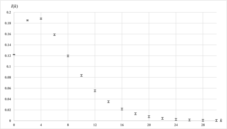
Figure 3. Bounds of $\ell(k)$ for $0\leq k\leq 30$. (Odd $k$'s are omitted.)

After proving an auxiliary result we will prove Theorem 1.2.

Lemma 3.21.

$\sum_{i=0}^{\infty}i\cdot\ell(i)=6$.

Proof.

$$\sum_{i=0}^{\infty}i\cdot\ell(i) \ =\ \lim\limits_{n\to\infty}\sum_{i=0}^{\infty}i\cdot P_{n}^{\text{M}}(i)$$

$$\ =\ \lim\limits_{n\to\infty}\sum_{i=0}^{\infty}\frac{1}{2^{n}}(2n-1-(2n-1-i))\cdot\#(S\subseteq[n]:|S-S|=2n-1-i)$$

$$\ =\ \lim\limits_{n\to\infty}(\frac{1}{2^{n}}(2n-1)2^{n}-\frac{1}{2^{n}}\sum_{i=0}^{\infty}i\#(S\subseteq[n]:|S-S|=i))$$

$$\ =\ \lim\limits_{n\to\infty}(2n-1-\frac{1}{2^{n}}\sum_{S\subseteq[n]}|S-S|)$$

$$\ =\ 6\text{ (by Theorem 3 of \cite[cite]{[\@@bibref{}{MO}{}{}]}{}).}$$ (3.14)

∎

Theorem 3.22.

For all $k\neq 4$, $\ell(k)<\ell(4)$.

Proof.

Theorem 1.3 proves the case for $k<12$. When $k\geq 12$, by Lemma 3.5 and 3.21,

$$2(k-6)\cdot\ell(k) \ <\ \sum_{i=k}^{\infty}(k-6)\cdot\ell(i)$$

$$\ <\ \sum_{i=6}^{\infty}(i-6)\cdot\ell(i)$$

$$\ =\ \sum_{i=0}^{\infty}(i-6)\cdot\ell(i)+6\ell(0)+4\ell(2)+2\ell(4)$$

$$\ <\ \sum_{i=0}^{\infty}i\cdot\ell(i)-6\sum_{i=0}^{\infty}\ell(i)+(6+4+2)\ell(4)$$

$$\ =\ 12\ell(4).$$ (3.15)

Thus $\Rightarrow\ell(k)<\ell(4)$. ∎

Proof of Theorem 1.2.

The theorem follows from Theorem 3.22 and Remark 3.3. ∎

Remark 3.23.

Theorem 1.2 gives a partial answer to Question A.2; the rather strange occurrence of $P_{n}^{\text{M}}(2)=P_{n}^{\text{M}}(4)$ happens only finitely many times.

3.4. About rulers

Definition 3.24.

A ruler of length $L$ is any subset $R\subseteq\{0,\dots,L\}$. It is complete if it can measure every distance shorter or equal to its length; that is, $\{0,...,L\}\subseteq R-R$.

Lemma 3.25.

Let $a_{n}$ be the number of complete rulers of length $n$; then $a_{n-1}\sim\ell(0)\cdot 2^{n}$.

Proof.

$S\subseteq[n]$ is a complete ruler of length $n-1$ iff $|S-S|=2n-1$, so the number of complete rulers of length $n-1$ is equal to $P_{n}^{\text{M}}(0)\cdot 2^{n}$, which goes to $\ell(0)\cdot 2^{n}$. ∎

Proof of Theorem 1.4.

The claim follows from Lemma 3.25 and Theorem 3.20. Here $c=2\ell(0)$. ∎

4. Conjectures

Intuitively, when $k\lll n$, randomly choosing $k$ elements from $[n]$ usually gives $|S-S|=k(k-1)+1$. On the other hand, to have $|S-S|=k(k-1)+3$ requires a maximal appearance of coincidences (repeated differences). Hence we have the following conjecture about the divots in $P_{n}^{\text{H}}$.

Conjecture 4.1.

For every $k>1$, $k(k-1)+3$ is a divot of $P_{n}^{\text{H}}$ for sufficiently large $n$. Furthermore, they are the only divots.

We also noticed that once a divot appears in $P_{n}^{\text{H}}$, it seems to never move again:

Conjecture 4.2.

If $k$ is a divot of $P_{n}^{\text{H}}$ for $n=n_{1}$, then it is also a divot for any $n>n_{1}$.

About missing differences, we proved Theorem 1.2 by limits, hence not giving an explicit threshold $N$ such that every $n\geq N$ satisfies Observation 3. Experimental data suggest that 15 might be enough already, so we guess:

Conjecture 4.3.

For all $n\geq 15$, $\forall k\neq 4$, $P_{n}^{\text{M}}(4)>P_{n}^{\text{M}}(k)$.

Recall that in Theorem 1.3, we compared the limiting probabilities of missing 0, 2, 4, 6, 8 and 10 differences, and found no divot. What about missing 12, or more? In fact, any two limiting probabilities can be approximated to be arbitrarily precise using our method, but we couldn't bound infinite many of them at the same time. Both intuition and experimental data seem to suggest that the decay after $\ell(4)$ should go on forever. Thus, we leave the following conjecture.

Conjecture 4.4.

In fact, $\ell(4)>\ell(2)>\ell(6)>\ell(0)>\ell(8)>\ell(10)>\ell(12)>\cdots$. In other words, the sequence $\ell$ has no divots.

Appendix A Distribution of $|S-S|$ when $n\leq 36$

Table 2. Number of $S\subseteq[n]$ with $|S-S|=k$. ($n\leq 24$)

	0	1	2	3	4	5	6	7	8	9	10	11	12	13	14	15	16	17	18	19	20	21	22	23	24
0	1	1	1	1	1	1	1	1	1	1	1	1	1	1	1	1	1	1	1	1	1	1	1	1	1
1	0	1	2	3	4	5	6	7	8	9	10	11	12	13	14	15	16	17	18	19	20	21	22	23	24
3	0	0	1	3	6	10	15	21	28	36	45	55	66	78	91	105	120	136	153	171	190	210	231	253	276
5	0	0	0	1	2	4	6	9	12	16	20	25	30	36	42	49	56	64	72	81	90	100	110	121	132
7	0	0	0	0	3	8	17	31	51	77	112	155	208	272	348	436	539	656	789	939	1107	1293	1500	1727	1976
9	0	0	0	0	0	4	10	17	27	43	62	85	113	148	189	236	289	352	423	501	588	687	795	913	1042
11	0	0	0	0	0	0	9	25	47	77	113	170	237	319	413	531	666	825	1000	1206	1430	1691	1970	2289	2630
13	0	0	0	0	0	0	0	17	49	97	169	269	409	606	863	1195	1607	2115	2735	3492	4393	5450	6690	8130	9790
15	0	0	0	0	0	0	0	0	33	93	177	275	402	549	730	967	1238	1562	1932	2355	2829	3345	3946	4613	5343
17	0	0	0	0	0	0	0	0	0	63	187	377	629	973	1417	1978	2688	3628	4765	6151	7794	9781	12089	14774	17861
19	0	0	0	0	0	0	0	0	0	0	128	377	747	1228	1850	2642	3633	4849	6340	8278	10580	13381	16603	20474	24909
21	0	0	0	0	0	0	0	0	0	0	0	248	747	1509	2507	3770	5338	7271	9641	12469	15909	20315	25533	31893	39392
23	0	0	0	0	0	0	0	0	0	0	0	0	495	1472	2975	4999	7519	10654	14499	19129	24681	31221	38903	48354	59263
25	0	0	0	0	0	0	0	0	0	0	0	0	0	988	2975	6022	10104	15278	21596	29249	38430	49408	62377	77572	95318
27	0	0	0	0	0	0	0	0	0	0	0	0	0	0	1969	5911	11985	20192	30501	43062	58148	76121	97667	123155	153424
29	0	0	0	0	0	0	0	0	0	0	0	0	0	0	0	3911	11880	24103	40524	61350	86236	115893	150319	190510	236824
31	0	0	0	0	0	0	0	0	0	0	0	0	0	0	0	0	7857	23734	48377	81542	123470	174352	234160	304245	385858
33	0	0	0	0	0	0	0	0	0	0	0	0	0	0	0	0	0	15635	47474	96676	162994	246765	347050	465537	602109
35	0	0	0	0	0	0	0	0	0	0	0	0	0	0	0	0	0	0	31304	94885	193562	326913	494449	696108	931109
37	0	0	0	0	0	0	0	0	0	0	0	0	0	0	0	0	0	0	0	62732	190623	388606	656644	993569	1396647
39	0	0	0	0	0	0	0	0	0	0	0	0	0	0	0	0	0	0	0	0	125501	380805	776640	1312446	1985532
41	0	0	0	0	0	0	0	0	0	0	0	0	0	0	0	0	0	0	0	0	0	250793	763402	1557467	2633237
43	0	0	0	0	0	0	0	0	0	0	0	0	0	0	0	0	0	0	0	0	0	0	503203	1528095	3117611
45	0	0	0	0	0	0	0	0	0	0	0	0	0	0	0	0	0	0	0	0	0	0	0	1006339	3061916
47	0	0	0	0	0	0	0	0	0	0	0	0	0	0	0	0	0	0	0	0	0	0	0	0	2014992
49	0	0	0	0	0	0	0	0	0	0	0	0	0	0	0	0	0	0	0	0	0	0	0	0	0

Table 3. Number of $S\subseteq[n]$ with $|S-S|=k$. ($24\leq n\leq 36$)

	24	25	26	27	28	29	30	31	32	33	34	35	36
0	1	1	1	1	1	1	1	1	1	1	1	1	1
1	24	25	26	27	28	29	30	31	32	33	34	35	36
3	276	300	325	351	378	406	435	465	496	528	561	595	630
5	132	144	156	169	182	196	210	225	240	256	272	289	306
7	1976	2248	2544	2864	3211	3584	3985	4415	4875	5365	5888	6443	7032
9	1042	1184	1338	1504	1682	1876	2084	2305	2541	2795	3064	3349	3651
11	2630	3010	3419	3876	4357	4886	5443	6060	6707	7410	8143	8940	9776
13	9790	11699	13868	16325	19094	22202	25674	29543	33832	38569	43786	49515	55787
15	5343	6158	7029	7980	9024	10164	11384	12696	14093	15597	17216	18941	20767
17	17861	21464	25554	30192	35439	41365	47972	55334	63485	72583	82597	93598	105615
19	24909	30034	35835	42560	50164	58778	68336	79218	91199	104572	119214	135569	153328
21	39392	48297	58729	70921	85023	101393	120236	141992	166842	195124	227418	263837	304894
23	59263	72166	86779	103803	122773	144495	168711	195948	226062	259777	297046	338522	383708
25	95318	116803	141545	170669	203518	241453	283954	332047	385486	445578	511668	585268	666132
27	153424	188936	230785	281634	340918	411385	492735	587687	696368	821738	964188	1126614	1309990
29	236824	290286	351743	422400	502848	598252	705828	831558	972438	1134483	1314383	1519559	1747229
31	385858	480260	589088	713474	855957	1018020	1202962	1419676	1664732	1947773	2265195	2627654	3032028
33	602109	759570	939048	1145157	1379205	1646202	1948206	2289594	2673659	3121284	3619723	4191609	4824889
35	931109	1202343	1512270	1865592	2266137	2720935	3236533	3821295	4483176	5231412	6075752	7058965	8161491
37	1396647	1867806	2404100	3013664	3697776	4468556	5330593	6293553	7368022	8567388	9903780	11391366	13047575
39	1985532	2792117	3726584	4795360	5994044	7342144	8845276	10520512	12382684	14456863	16757210	19313503	22151419
41	2633237	3984017	5596451	7469425	9586795	11966365	14608625	17543417	20782662	24369445	28318130	32680465	37482058
43	3117611	5270104	7970998	11195574	14913983	19131301	23822819	29022146	34739876	41039669	47936336	55509344	63800433
45	3061916	6244117	10557091	15968677	22417023	29862931	38239392	47566626	57804101	69047026	81288502	94666428	109216351
47	2014992	6125358	12494664	21122722	31935586	44822674	59651353	76346946	94783970	115036473	137031262	160950680	186816887
49	0	4035985	12278446	25038586	42321005	63983506	89749444	119386846	152607226	189351319	229343035	272803379	319629353
51	0	0	8080448	24564954	50090752	84658919	127967673	179465499	238552257	304816636	377630128	456991110	542473471
53	0	0	0	16169267	49200792	100303312	169496641	256144840	359073831	477185749	609113912	754212597	911317415
55	0	0	0	0	32397761	98478615	200765677	339187677	512453496	718291220	953949620	1217261287	1505590283
57	0	0	0	0	0	64826967	197164774	401837351	678805584	1025433250	1436715877	1907636501	2432498687
59	0	0	0	0	0	0	129774838	394536002	804070333	1358091161	2051059855	2873264810	3813305230
61	0	0	0	0	0	0	0	259822143	789993459	1609586119	2717986051	4104228068	5747795503
63	0	0	0	0	0	0	0	0	520063531	1580640910	3220331421	5437313809	8208838614
65	0	0	0	0	0	0	0	0	0	1040616486	3163602123	6444236200	10879185718
67	0	0	0	0	0	0	0	0	0	0	2083345793	6330608624	12894355828
69	0	0	0	0	0	0	0	0	0	0	0	4168640894	12668987317
71	0	0	0	0	0	0	0	0	0	0	0	0	8342197304
73	0	0	0	0	0	0	0	0	0	0	0	0	0

Remark A.1.

Denoting the table by $T$, $T_{n,k}/2^{n}=P_{n}^{\text{H}}(k)=P_{n}^{\text{M}}(2n-1-k)$.

Question A.2.

Observe that when $n=3,11,12,14$, $P_{n}^{\text{M}}(2)=P_{n}^{\text{M}}(4)$. Such frequent repetition of large numbers doesn't look so random. Is there any reason behind it? Will it happen again?

Appendix B Code for Estimating $j(2k)$

⬇

#include <stdio.h>

#include <time.h>

#include <math.h>

long long cnts[100];

int main() {

int m = 23, d; // Measure prob of missing n-1, ... n-m diffs

clock_t begin = clock();

double j[100], error = pow(0.75, m+1) * 16 / 9;

long long cnt, r1 = (1LL << 2*m), r2 = 2*m-1;

for(long long S = (1LL << (2*m-1)) + 1; S < r1; S+=2) {

cnt = 0;

for(d = m; d < r2; d++) if(!(S & (S >> d))) cnt++;

cnts[cnt]++;

}

for(int i=0; i<m; i++) {

j[2*i] = 1.0 * cnts[i] / pow(2, 2*m-2);

printf("j(%d) = %f+-%e\t(G%d = %lld/2^%d)\n", 2*i,

j[2*i], error, i, cnts[i], 2*m-2);

}

clock_t end = clock();

double time_spent = (double)(end - begin) / CLOCKS_PER_SEC;

printf("\nj(0)/4 < (%f+%f)/4 = %f <? %f = %f-%f < j(4).\nj(0)+ j(2) > %f+%f-2*%f = %f >? %f = 4(%f+%f) = 4j(6).\n",

j[0], error, j[0]/4+error/4, j[4]-error, j[4], error,

j[0], j[2], error, j[0]+j[2]-2*error, j[6]*4+error*4,

j[6], error);

printf("In %f sec.\n", time_spent);

return 0;

}

Remark B.1.

The algorithm is $\Omega(4^{m}m^{2})$. When $m=23$, it runs for 92.73 hours on our laptop. In fact, even when $m=18$, which takes only 3 minutes to run, the results could already establish $\ell(2)-\ell(4)<0$, and hence Theorem 1.2, although it's not strong enough to show that $\ell(0)>\ell(8)$. The reader is welcome to confirm our calculations or achieve better bounds.

References

- [AMMS] M. Asada, S. Manski, S. J. Miller and H. Suh, Fringe pairs in generalized MSTD sets, International Journal of Number Theory 13 (2017), no. 10, 2653–2675.
- [BELM] A. Bower, R. Evans, V. Luo and S. J. Miller, Coordinate sum and difference sets of -dimensional modular hyperbolas, INTEGERS #A31, 2013, 16 pages.
- [CLMS] H. Chu, N. Luntzlara, S. J. Miller and L. Shao, Generalizations of a Curious Family of MSTD Sets Hidden By Interior Blocks, to appear in Integers.
- [CMMXZ] H. Chu, N. McNew, S. J. Miller, V. Xu and S. Zhang, When Sets Can and Cannot Have MSTD Subsets, Journal of Integer Sequences 21 (2018), Article 18.8.2.
- [DKMMW] T. Do, A. Kulkarni, S. J. Miller, D. Moon and J. Wellens, Sums and Differences of Correlated Random Sets, Journal of Number Theory 147 (2015), 44–68.
- [DKMMWW] T. Do, A. Kulkarni, S. J. Miller, D. Moon, J. Wellens and J. Wilcox, Sets Characterized by Missing Sums and Differences in Dilating Polytopes, Journal of Number Theory 157 (2015), 123–153.
- [He] P. V. Hegarty, Some explicit constructions of sets with more sums than differences, Acta Arith. 130 (2007), 61–77.
- [HM] P. V. Hegarty and S. J. Miller, When almost all sets are difference dominated, Random Structures Algorithms 35 (2009), 118–136.
- [HLM] A. Hemmady, A. Lott and S. J. Miller, When almost all sets are difference dominated in , Integers 17 (2017), Paper No. A54, 15 pp.
- [ILMZ] G. Iyer, O. Lazarev, S. J. Miller and L. Zhang, Generalized More Sums Than Differences Sets, Journal of Number Theory 132 (2012), no. 5, 1054–1073.
- [LMO] O. Lazarev, S. J. Miller and K. O'Bryant, Distribution of Missing Sums in Sumsets, Experimental Mathematics 22 (2013), no. 2, 132–156.
- [MA] J. Marica, On a conjecture of Conway, Canad. Math. Bull. 12 (1969), 233–234.
- [MO] G. Martin and K. O'Bryant, Many sets have more sums than differences, Additive Combinatorics, Providence, RI, 2007, 287–305.
- [MOS] S. J. Miller, B. Orosz and D. Scheinerman, Explicit constructions of infinite families of MSTD sets, Journal of Number Theory 130 (2010), 1221–1233.
- [MP] S. J. Miller and C. Peterson, A geometric perspective on the MSTD question, Discrete and Computational Geometry 62 (2019), no. 4, 832–855.
- [MS] S. J. Miller and D. Scheinerman, Explicit constructions of infinite families of MSTD sets, Additive Number Theory: Festschrift In Honor of the Sixtieth Birthday of Melvyn B. Nathanson (David Chudnovsky and Gregory Chudnovsky, editors), Springer-Verlag, 2010.
- [MV] S. J. Miller and K. Vissuet, Most Subsets are Balanced in Finite Groups, Combinatorial and Additive Number Theory, CANT 2011 and 2012 (Melvyn B. Nathanson, editor), Springer Proceedings in Mathematics & Statistics (2014), 147–157.
- [MXZ] S. Miller, V. Xu and X. Zhang, MSTD Subsets and Properties of Divots in the Distribution of Missing Sums, Combinatorial and Additive Number Theory, 05/26/16.
- [Na1] M. B. Nathanson, Problems in additive number theory I, Additive combinatorics, Providence, RI, 2007, 263–270.
- [Na2] M. B. Nathanson, Sets with more sums than differences, Integers 7 (2007), #A5.
- [Ru1] I. Z. Ruzsa, On the cardinality of and , Combinatorics Year, North-Holland-Bolyai Trsulat, Keszthely, 1978, 933–938.
- [Ru2] I. Z. Ruzsa, Sets of sums and differences, Séminaire de Théorie des Nombres de Paris, Birkhäuser, Boston, 1984, 267–273.
- [Ru3] I. Z. Ruzsa, On the number of sums and differences, Acta Math. Sci. Hungar. 59 (1992), 439–447.
- [Zh1] Y. Zhao, Constructing MSTD sets using bidirectional ballot sequences, J. Number Theory 130 (2010), 1212–1220.
- [Zh2] Y. Zhao, Sets characterized by missing sums and differences, J. Number Theory 131 (2011), 2107–2134.