Normal-normal resonances in a double Hopf bifurcation

Abstract

We investigate the stability loss of invariant $n$–dimensional quasi-periodic tori during a double Hopf bifurcation, where at bifurcation the two normal frequencies are in normal-normal resonance. Invariants are used to analyse the normal form approximations in a unified manner. The corresponding dynamics form a skeleton for the dynamics of the original system. Here both normal hyperbolicity and kam theory are being used.

1 Introduction

Double Hopf bifurcations of $n$–dimensional tori in their simplest form occur in $n+4$ dimensions. Therefore we consider a family of vector fields on an $(n+4)$–dimensional manifold that leave invariant a family of conditionally periodic $n$–tori. Locally around the tori the dynamics are then of the form

$$\dot{x} \;\;=\;\;\omega(\mu)\;+\;\mathcal{O}(z),$$ (1a)

$$\dot{z} \;\;=\;\;\Omega(\mu)\,z\;+\;\mathcal{O}(z^{2}),$$ (1b)

where $\mu\in\mathbb{R}^{s}$ denotes the parameter. We assume the tori to be reducible to Floquet form and that the double Hopf bifurcation occurs at $\mu=0$. The eigenvalues of $\Omega=\Omega(\mu)$ are the Floquet exponents $\beta_{j}(\mu)\pm{\rm i}\alpha_{j}(\mu)$, $\alpha_{j},\beta_{j}\in\mathbb{R}$ and $j=1,2$, of the invariant torus $\mathbb{T}^{n}\times\{0\}$.

For $\mu=0$ the tori are at a double Hopf singularity if $\beta_{j}(0)=0$ and $\alpha_{j}(0)\neq 0$ for $j=1,2$. Within this singularity, the normal frequencies $\alpha_{j}(0)$ are at normal-normal resonance if moreover

$$\ell_{2}\alpha_{1}(0)\;\;=\;\;\ell_{1}\alpha_{2}(0)$$ (2)

for some $0\neq\ell=(\ell_{1},\ell_{2})\in\mathbb{Z}^{2}$. The aim of this article is to study the dynamics of the family (1) near such resonances.

The normal linear part of (1) is obtained by truncating the $\mathcal{O}(z)$ and $\mathcal{O}(z^{2})$ terms in (1a) and (1b), respectively. The flow of this normal linear part is equivariant with respect to a $\mathbb{T}^{n}\times\mathbb{T}^{2}$ action and in the resonant case (2) the symmetry group is even larger (the symmetry group is maximal in the case $\alpha_{1}(0)=\alpha_{2}(0)=0$, which we do not consider further). The aim of normal form theory is to push the symmetry to higher order terms by successive transformations, compare with [25]. In the non-resonant case the entire $\mathbb{T}^{n}\times\mathbb{T}^{2}$ symmetry is inherited by the normalised dynamics. However, in the present normal-normal resonant case the normalised terms only inherit a $\mathbb{T}^{n}\times\mathbb{T}^{1}$ symmetry.

We apply finitely many normalising transformations so to obtain a $\mathbb{T}^{n}\times\mathbb{T}^{1}$ symmetric truncation. In particular, the coefficients in this truncation are $x$–independent. This decouples the normal dynamics from the internal dynamics. The normal dynamics retains a $\mathbb{T}$ symmetry. After reducing this out, a three-dimensional system remains. Equilibria of this reduced system correspond to either $n$–dimensional or $(n+1)$–dimensional invariant tori in the normal form truncation. The full system is a small perturbation of this truncation; to assess the impact of the higher order remainder terms, we invoke both normal hyperbolicity and kam theory.

In (2) we may assume that $0<\ell_{1}\leq\ell_{2}$ and $\alpha_{j}(0)>0$, $j=1,2$, if necessary by relabeling the frequencies and scaling the variables. We restrict to weak resonances: these are resonances where in (2) we have $0<\ell_{1}<\ell_{2}$. This rules out the strongly resonant case $\ell=(1,1)$.

Remarks.

1. Instead of starting in $n+4$ dimensions we could also take as starting point a family of vector fields on an $(n+m)$–dimensional manifold. However, our first step would then be to split the normal spectrum of the bifurcating $n$–torus into the $4$ purely imaginary eigenvalues $\pm{\rm i}\alpha_{1}(0),\pm{\rm i}\alpha_{2}(0)$ and the remaining $m-4$ hyperbolic eigenvalues and to then perform a restriction to the resulting $(n+4)$–dimensional normally hyperbolic invariant manifold on which we have the situation sketched above. We note that this procedure generically leads to a finitely differentiable system.

2. We generally assume our systems to be real analytic, which facilitates the application of kam theory. However, for applications on centre manifolds finitely differentiable versions of kam theory are available [9, 11].

3. One of the improvements of normalisation theory in the analytic setting is that the remainder term can be made exponentially small [8, 7] in the perturbation parameter. In the finitely differentiable case this would be only polynomially small.

1.1 Previous work

The resonant double Hopf bifurcation has already been studied by many authors. The strong $1{:}1$ resonance, to which we do not contribute, has been studied in [41, 23, 36]. Of the weak resonances, the $1{:}2$ resonance has gotten the most attention [28, 32, 29, 34, 44, 38]; next to it, the $1{:}3$ resonance [34] and the $2{:}3$ resonance [37, 39] have been investigated as well.

Most previous work has been on the case $n=0$ where it is an equilibrium that has two (normal) frequencies and we therefore also speak of $1$–dimensional invariant tori instead of periodic orbits. The non-resonant case where only $\beta_{1}(0)=\beta_{2}(0)=0$, but $\alpha_{1}(0)$ and $\alpha_{2}(0)$ do not satisfy (2) for any $0\neq\ell\in\mathbb{Z}^{2}$, has a $\mathbb{T}^{2}$ symmetry instead of a $\mathbb{T}^{1}$ symmetry in the normal forms. Reduction leads to a $2$–dimensional basis system and the dynamics of this $2$–dimensional normal form was already laid out in [25]. However, it took until [33] for a formal proof of persistence of the resulting invariant tori under perturbation from the normal form back to the original system.

To summarise the literature on the weakly resonant case (again mostly $n=0$), it is convenient to call ‘resonance droplet’ the part of parameter space for which $1$–dimensional invariant tori with non-zero amplitudes exist. This corresponds for instance with the ‘mixed modes’ situation of Knobloch and Proctor [28]. They made an extensive local study of that part of the boundary of the resonance droplet of the $1{:}2$ resonant double Hopf bifurcation where a $1$–dimensional torus bifurcates to a $2$–dimensional torus, checking all configurations and determining global bifurcations. LeBlanc and Langford [32] used for the same Hopf bifurcation Lyapunov-Schmidt theory and singularity theory to study only these $1$–dimensional tori. Luongo et al. [34] applied a multiple timescale analysis to the resonant $1{:}2$ and $1{:}3$ double Hopf bifurcation in a straightforward perturbative approach. They perform an extensive numerical analysis, finding several instances of resonance droplets. Volkov [44] takes $n\geq 2$ and studies the persistence of $n$–dimensional quasi-periodic tori at a $1{:}2$ double Hopf normal resonance. Finally, Revel et al. [37, 38, 39] study $1{:}2$ and $2{:}3$ resonant double Hopf bifurcations numerically.

Remarks.

1. Already in the work of Guckenheimer and Holmes [25] on the non-resonant case the treatment was devided into $12$ cases. In this paper we focus on the case labeled VIa in [25], where a subordinate Hopf bifurcation takes place after reduction of the $\mathbb{T}^{n}\times\mathbb{T}^{2}$ symmetry. Next to this examplary case we note that our approach also applies to all other cases as treated by Knobloch and Proctor [28].

2. Next to the subordinate bifurcations of co-dimension $1$ we also meet bifurcations of co-dimension $2$ that act as organising centers of the dynamics. These are subordinate resonant Hopf bifurcations, fold-Hopf bifurcations, and blue sky bifurcations. Also compare with [5, 12]. The fold-Hopf bifurcation does not seem to have been noticed earlier in the literature and a full treatment is outside the present scope, so we refer to [9].

3. In the sequel we introduce the invariants $\tau_{j}$, $j=1,2,3,4$. Here $\tau_{1}$ and $\tau_{2}$ generate the $\mathbb{T}^{2}$–symmetry, while $\tau_{3}$ and $\tau_{4}$ are a global version of the resonant angle. This systematic approach is standard for Hamiltonian systems, and has already been used in [28] for the $1{:}2$ resonance. We shall encounter $3$–dimensional versions of the Arnol’d resonance tongues as met in families of circle diffeomorphisms. The intersection with a transverse plane has the form of a droplet, see figures 4 and 5 below.

1.2 Outline

Our contribution is to establish the geometry of the resonance droplet in a generic three-parameter unfolding of a general $\ell_{1}{:}\ell_{2}$ resonant double Hopf bifurcation, excluding only the strongly resonant $1{:}1$ situation. We also put all occurring subordinate Hopf bifurcations on an equal footing, but leave the occurring quasi-periodic fold-Hopf and heteroclinic bifurcations to future research.

To sketch our results we already refer to the bifurcation diagram in figure 1, which describes the truncated normal form after reduction of a $\mathbb{T}^{n}\times\mathbb{T}^{2}$ symmetry. From this the symmetric skeleton is reconstructed. The final step is to use perturbation theory back to the original system. This involves both normal hyperbolicity and kam theory.

2 Linear dynamics

Consider on the phase space $\mathbb{R}^{4}$ the system

$$\dot{z} \;\;=\;\;\Omega(\mu)z.$$ (3)

This is the normal part of the normal linear dynamics at the invariant $n$–torus $\mathbb{T}^{n}\times\{0\}$.

We assume that the $4$ eigenvalues of $\Omega(\mu)$ are of the form $\beta_{j}(\mu)\pm{\rm i}\alpha_{j}(\mu)$ and that they satisfy $\beta_{j}(0)=0$ and $\alpha_{j}(0)>0$, for $j=1,2$. Analogously to the internal frequency vector $\omega(\mu)$, the normal frequency vector of the invariant torus $\mathbb{T}^{n}\times\{0\}$ is $\alpha(\mu)=(\alpha_{1}(\mu),\alpha_{2}(\mu))$. Moreover, we assume that the normal frequencies are in normal-normal resonance (2). If necessary after rescaling time, it can be achieved that $\alpha_{1}(0)$ takes some given value, for instance $\alpha_{1}(0)=\ell_{1}$ (whence $\alpha_{2}(0)=\ell_{2}$). Finally, we can assume that $\gcd(\ell_{1},\ell_{2})=1$. Normal-normal resonances at Hopf bifurcation generically may occur in families depending on three or more parameters.

Introducing complex variables $Z_{j}=z_{2j-1}+{\rm i}z_{2j}$, $j=1,2$, at $\mu=0$ the system (3) takes the form

$$\dot{Z}_{j}\;\;=\;\;{\rm i}\alpha_{j}(0)Z_{j}.$$

Under the linear flow there are four basic invariants

$$\tau_{1} \;=\;{\textstyle\frac{1}{2}}Z_{1}\bar{Z}_{1},\quad \tau_{3} \;=\;\frac{{\mathop{\rm Re}}\,Z_{1}^{\ell_{2}}\bar{Z}_{2}^{\ell_{1}}}{\ell_{1}!\ell_{2}!},$$ (4a)

$$\tau_{2} \;=\;{\textstyle\frac{1}{2}}Z_{2}\bar{Z}_{2}, \tau_{4} \;=\;\frac{{\mathop{\rm Im}}\,Z_{1}^{\ell_{2}}\bar{Z}_{2}^{\ell_{1}}}{\ell_{1}!\ell_{2}!},$$ (4b)

i.e. all other functions that are invariant under the flow of (3) can be expressed as functions of the $\tau_{k}$. These invariants are related by the syzygy

$$\tau_{1}^{\ell_{2}}\tau_{2}^{\ell_{1}}\,-\,G_{\ell}(\tau_{3}^{2}+\tau_{4}^{2})\;=\;0,\quad G_{\ell}\;=\;\frac{(\ell_{1}!)^{2}(\ell_{2}!)^{2}}{2^{\ell_{1}+\ell_{2}}}.$$

The first two invariants are related to polar co-ordinates by the formula $Z_{j}=\sqrt{2\tau_{j}}{\rm e}^{{\rm i}\phi_{j}}$. At $\mu=0$ the angles $\phi_{j}$ have the equations of motion

$$\dot{\phi}_{j}\;\;=\;\;\alpha_{j}(0),\quad j=1,2.$$

As the frequencies are in resonance, the orbits foliate each $\mathbb{T}^{2}$ into closed $1$–dimensional orbits. This is brought out explicitly by introducing resonance-adapted angles $(\theta,\vartheta)$ such that

$$\theta \;\;=\;\;\ell_{2}\phi_{1}\;-\;\ell_{1}\phi_{2},$$ (5a)

$$\vartheta \;\;=\;\;m_{1}\phi_{1}\;+\;m_{2}\phi_{2}.$$ (5b)

While the right hand side of (5b) is clearly the inner product $\langle m\mid\phi\rangle$, we define $\ell^{\perp}:=(\ell_{2},-\ell_{1})$ to write the right hand side of (5a) as $\langle\ell^{\perp}\mid\phi\rangle$

In order that the equations (5) provide a torus diffeomorphism, the $m_{j}$ have to be chosen such that the matrix $\left({}^{\ell_{2}}_{m_{1}}{}^{-\ell_{1}}_{m_{2}}\right)$ is unimodular. This is possible as $\gcd(\ell_{1},\ell_{2})=1$. Note that

$$\tau_{3}\;=\;\sqrt{G_{\ell}\tau_{1}^{\ell_{2}}\tau_{2}^{\ell_{1}}}\cos\theta\quad\mbox{and}\quad\tau_{4}\;=\;\sqrt{G_{\ell}\tau_{1}^{\ell_{2}}\tau_{2}^{\ell_{1}}}\sin\theta\,.$$ (6)

In these variables, the linear dynamics are given by

$$\begin{array}[]{rcl}\dot{\tau}_{j}&=&0,\quad j=1,\ldots,4\\ \dot{\theta}&=&0\quad\mbox{(redundant)}\\ \dot{\vartheta}&=&m_{1}\alpha_{1}(0)\;+\;m_{2}\alpha_{2}(0)\;\;=\;\;1,\end{array}$$ (7)

making $\vartheta$ a ‘fast’ angle. In appropriate co-ordinates the linear family $\dot{z}=\Omega(\mu)z$ is given by

$$\Omega(\mu)\;\;=\;\;\begin{pmatrix}\beta_{1}(\mu)&-\alpha_{1}(\mu)&0&0\\ \alpha_{1}(\mu)&\beta_{1}(\mu)&0&0\\ 0&0&\beta_{2}(\mu)&-\alpha_{2}(\mu)\\ 0&0&\alpha_{2}(\mu)&\beta_{2}(\mu)\\ \end{pmatrix}\,.$$

In terms of the complex variables this simplifies, first to

$$\dot{Z}_{j}\;\;=\;\;(\beta_{j}(\mu)\,+\,{\rm i}\alpha_{j}(\mu))Z_{j},\quad j=1,2$$

and then to

$$\dot{Z}_{j} \;\;=\;\;({\rm i}\alpha_{j}(0)\,+\,\beta_{j}+{\rm i}\delta_{j})Z_{j}\,,$$

where the $\delta_{j}=\alpha_{j}(\mu)-\alpha_{j}(0)$ detune the normal frequencies and form, together with $\beta_{j}=\beta_{j}(\mu)$, $j=1,2$, the new independent parameters. In fact, we have passed to $\mu=(\delta_{1},\delta_{2},\beta_{1},\beta_{2},\nu)$, where $\nu\in\mathbb{R}^{s-4}$ is a mute parameter. According to [1] this is a versal unfolding.

3 Normal form

We now add the higher order terms to the linear system. On the phase space $\mathbb{T}^{n}\times\mathbb{R}^{4}$ the system becomes

$$\dot{x} \;\;=\;\;f(x,z,\mu) \;\;=\;\;\omega(\mu)\;+\;\tilde{f}(x,z,\mu),$$

$$\dot{z} \;\;=\;\;h(x,z,\mu) \;\;=\;\;\Omega(\mu)z\;+\;\tilde{h}(x,z,\mu),$$

where $\tilde{f}=\mathcal{O}(|z|)$ and $\tilde{h}=\mathcal{O}(|z|^{2})$. To this system are associated the vector field

$$X\;\;=\;\;f\partial_{x}\;+\;h\partial_{z}$$ (8)

and its normal linear part $L=\omega\partial_{z}+\Omega z\partial_{z}$. From the previous section we retain the assumptions on the eigenvalues of $\Omega(\mu)$ and the complex variables $Z_{j}$. In these terms, the system takes the form

$$\dot{x} \;\;=\;\;f(x,Z,\bar{Z},\mu) \;\;=\;\;\omega(\mu)\;+\;\tilde{f}(x,Z,\bar{Z},\mu),$$

$$\dot{Z}_{1} \;\;=\;\;h_{1}(x,Z,\bar{Z},\mu) \;\;=\;\;({\rm i}\alpha_{1}(0)+\beta_{1}+{\rm i}\delta_{1})Z_{1}\;+\;\tilde{h}_{1}(x,Z,\bar{Z},\mu),$$

$$\dot{Z}_{2} \;\;=\;\;h_{2}(x,Z,\bar{Z},\mu) \;\;=\;\;({\rm i}\alpha_{2}(0)+\beta_{2}+{\rm i}\delta_{2})Z_{2}\;+\;\tilde{h}_{2}(x,Z,\bar{Z},\mu)\,,$$

where $\mu_{1}=\delta_{1}$, $\mu_{2}=\delta_{2}$, $\mu_{3}=\beta_{1}$ and $\mu_{4}=\beta_{2}$ while the mute parameter $\nu$ has been dropped.

Theorem 3.1 (Normal Form)

Let $\ell\in\mathbb{Z}^{2}$ be such that $0<\ell_{1}<\ell_{2}$. Consider the real analytic vector field (8) where for $\kappa>n-1$ and $\Gamma>0$ the frequency vector $(\omega,\alpha)$ at $\mu=0$ satisfies the Diophantine conditions

$$\left|\langle k^{\prime}\mid\omega(0)\rangle\;+\;\langle\ell^{\prime}\mid\alpha(0)\rangle\right|\;\;\geq\;\;\frac{\Gamma}{(|k^{\prime}|+|\ell^{\prime}|)^{\kappa}}$$ (9)

for all $(k^{\prime},\ell^{\prime})\in\mathbb{Z}^{n}\times\mathbb{Z}^{2}$ except for $(k^{\prime},\ell^{\prime})=(0,\ell^{\perp})$ and its integer multiples. For given order $M\in\mathbb{N}$ of normalisation there is a diffeomorphism

$$\Phi\>:\>\>\mathbb{T}^{n}\times\mathbb{C}^{2}\times\mathbb{R}^{s} \longrightarrow\mathbb{T}^{n}\times\mathbb{C}^{2}\times\mathbb{R}^{s},$$

real analytic in $x$, $Z$, $\bar{Z}$ and $\mu$, close to the identity at $(Z,\mu)=(0,0)$, such that the following holds.

The vector field $X$ is transformed into normal form

$$\Phi_{*}X\;\;=\;\;N\;+\;R.$$ (10)

The lower order part $N$ is

$$N \;\;=\;\;\omega(0)\partial_{x}\;+\;({\rm i}\alpha_{1}(0)+\beta_{1}+{\rm i}\delta_{1})Z_{1}\partial_{Z_{1}}\;+\;({\rm i}\alpha_{2}(0)+\beta_{2}+{\rm i}\delta_{2})Z_{2}\partial_{Z_{2}}$$

$$\quad\;+\;\sum_{m}C^{0}_{m}\prod_{j=1}^{4}\tau_{j}^{m_{j}}\prod_{k=1}^{s}\mu_{k}^{m_{4+k}}\partial_{x}$$

$$\quad\;+\;\sum_{m}C^{1}_{m}\prod_{j=1}^{4}\tau_{j}^{m_{j}}\prod_{k=1}^{s}\mu_{k}^{m_{4+k}}Z_{1}\partial_{Z_{1}}$$

$$\quad\;+\;\sum_{m}C^{2}_{m}\prod_{j=1}^{4}\tau_{j}^{m_{j}}\prod_{k=1}^{s}\mu_{k}^{m_{4+k}}Z_{2}\partial_{Z_{2}}$$

$$\quad\;+\;\text{c.c.},$$

where c.c. is short for complex conjugate, $C^{j}_{m}\in\mathbb{C}$ and $m\in\mathbb{N}^{4+s}$ with

$$2\;\;\leq\;\;2(m_{1}+m_{2})\;+\;|\ell|(m_{3}+m_{4})\;+\;\sum_{j=1}^{s}m_{4+j}\;\;\leq\;\;M.$$

The remainder $R$ satisfies the estimate

$$R\;\;=\;\;O_{M+1}(|Z|,|\mu|)\partial_{x}\;+\;O_{M+1}(|Z|,|\mu)Z_{1}\partial_{Z_{1}}\;+\;O_{M+1}(|Z|,|\mu)Z_{2}\partial_{Z_{2}}.$$

The proof relies on a succession of normal form transformations, see e.g. [9]. Taking $M=\max(4,|\ell|)$, the lower order part $N$ of the normal form can be written in the form

$$\dot{x} \;\;=\;\;\omega(\mu)\;+\;\hat{f}(\tau_{1},\tau_{2},\mu)\;+\;a_{0}(\mu)\tau_{3}\;+\;c_{0}(\mu)\tau_{4},$$

$$\dot{Z}_{j} \;\;=\;\;\left({\rm i}\alpha_{j}(0)\,+\,\beta_{j}\,+\,{\rm i}\delta_{j}\,+\,p_{j}(\tau_{1},\tau_{2},\mu)\,+\,{\rm i}q_{j}(\tau_{1},\tau_{2},\mu)\right.$$

$$\qquad\left.\mbox{}+\,[a_{j}(\mu)+{\rm i}b_{j}(\mu)]\tau_{3}\,+\,[c_{j}(\mu)+{\rm i}d_{j}(\mu)]\tau_{4}\right)Z_{j},\quad j=1,2,$$

where $\hat{f}(0,0,\mu)=0$ and $p_{j}(0,0,\mu)=q_{j}(0,0,\mu)=0$ while $\tau_{3}$ and $\tau_{4}$ only enter linearly — that is what we mean by lower order part.

The form of these equations already suggests that after discarding the strong $1{:}1$ resonance there are still three distinct situations.

• The first case is $|\ell|=3$ — the $1{:}2$ resonance — where the terms $\tau_{3}$ and $\tau_{4}$ are larger than the terms $\tau_{1}^{2}$ and $\tau_{2}^{2}$.

• The second case is $|\ell|=4$ — the $1{:}3$ resonance — where these terms are of the same order of magnitude.

• The third case is $|\ell|\geq 5$ — higher order resonances — where the terms $\tau_{3}$ and $\tau_{4}$ are smaller than the terms $\tau_{1}^{2}$ and $\tau_{2}^{2}$.

4 Analysis of the truncated normal form

In the normal form vector field (10) we truncate the remainder $R$ so to obtain the $\mathbb{T}^{n}\times\mathbb{T}^{1}$ symmetric normal form truncation $N$. Reducing the $\mathbb{T}^{n}$ symmetry we obtain a normal dynamics on $\mathbb{R}^{4}$ that still has a $\mathbb{T}$ symmetry. By abuse of notation we denote this reduced vector field by $N$ as well.

Equilibria of the reduced $N$ usually are called relative equilibria. Observe that on $\mathbb{T}^{n}\times\mathbb{R}^{4}$ these correspond to invariant $n$–tori. In fact the normal system behaves like in the case where $n=0$. For this reason the relative equilibria sometimes are referred to as $0$–tori.

Similarly periodic orbits of the reduced $N$ usually are called relative periodic orbits. Observe that on $\mathbb{T}^{n}\times\mathbb{R}^{4}$ these correspond to invariant $(n+1)$–tori. For this reason the relative periodic orbits sometimes are referred to as $1$–tori.

4.1 Passing to invariants

Recall formula (6) that relates $\tau_{3}$ and $\tau_{4}$ to $\tau_{1},\tau_{2}$ and the resonant angle $\theta$. Compared to polar co-ordinates, the invariants $\tau_{1}$ and $\tau_{2}$ take the part of the radii, whereas $\tau_{3}$ and $\tau_{4}$ take the part of $\cos\theta$ and $\sin\theta$.

Expressed in invariants, the normal form truncation $N$ reads as

$$\dot{\tau}_{1} \;\;=\;\;2\left(\beta_{1}+p_{1}+a_{1}\tau_{3}+c_{1}\tau_{4}\right)\tau_{1},$$

$$\dot{\tau}_{2} \;\;=\;\;2\left(\beta_{2}+p_{2}+a_{2}\tau_{3}+c_{2}\tau_{4}\right)\tau_{2},$$

$$\dot{\tau}_{3} \;\;=\;\;\left(\ell_{2}(\beta_{1}+p_{1}+a_{1}\tau_{3}+c_{1}\tau_{4})\,+\,\ell_{1}(\beta_{2}+p_{2}+a_{2}\tau_{3}+c_{2}\tau_{4})\right)\tau_{3}$$

$$\quad-\left(\ell_{2}(\delta_{1}+q_{1}+b_{1}\tau_{3}+d_{1}\tau_{4})\,-\,\ell_{1}(\delta_{2}+q_{2}+b_{2}\tau_{3}+d_{2}\tau_{4})\right)\tau_{4},$$

$$\dot{\tau}_{4} \;\;=\;\;\left(\ell_{2}(\delta_{1}+q_{1}+b_{1}\tau_{3}+d_{1}\tau_{4})\,-\,\ell_{1}(\delta_{2}+q_{2}+b_{2}\tau_{3}+d_{2}\tau_{4})\right)\tau_{3}$$

$$\quad+\left(\ell_{2}(\beta_{1}+p_{1}+a_{1}\tau_{3}+c_{1}\tau_{4})\,+\,\ell_{1}(\beta_{2}+p_{2}+a_{2}\tau_{3}+c_{2}\tau_{4})\right)\tau_{4}.$$

We introduce

$$A\;=\;\begin{pmatrix}a_{1}&c_{1}\\ a_{2}&c_{2}\end{pmatrix},\quad B\;=\;\begin{pmatrix}b_{1}&d_{1}\\ b_{2}&d_{2}\end{pmatrix}.$$

Preparing for a Taylor expansion of the right hand side, we also introduce

$$p_{ij}(\mu) \;=\;\frac{\partial p_{i}}{\partial\tau_{j}}(0,0,\mu),\quad P(\mu)\;=\;\begin{pmatrix}p_{11}(\mu)&p_{12}(\mu)\\ p_{21}(\mu)&p_{22}(\mu)\end{pmatrix}$$

as well as

$$q_{ij}(\mu) \;=\;\frac{\partial q_{i}}{\partial\tau_{j}}(0,0,\mu),\quad Q(\mu)\;=\;\begin{pmatrix}q_{11}(\mu)&q_{12}(\mu)\\ q_{21}(\mu)&q_{22}(\mu)\end{pmatrix}.$$

We zoom in on the origin of $\mathbb{R}^{4}$ by scaling time, the invariants and the parameters as

$$t \;=\;\varepsilon^{-2}\tilde{t},\quad\tau_{j}\;=\;\varepsilon^{2}\sigma_{j},\quad\tau_{j+2}\;=\;\varepsilon^{|\ell|}\psi_{j},\quad\beta_{j}\;=\;\varepsilon^{2}\gamma_{j},\quad\delta_{j}\;=\;\varepsilon^{2}\eta_{j},\quad j=1,2,$$

thereby splitting $\tau$ into the amplitude $\sigma$ and the phase $\psi$ (recall from (6) that $\psi$ is a scaled version of $\cos\theta$ and $\sin\theta$). This allows to introduce $\tilde{p}$ and $\tilde{q}$ by

$$p(\varepsilon^{2}\sigma,\mu) \;\;=\;\;\varepsilon^{2}P(\mu)\sigma\;+\;\varepsilon^{4}\tilde{p}(\sigma,\varepsilon^{2},\mu),$$

$$q(\varepsilon^{2}\sigma,\mu) \;\;=\;\;\varepsilon^{2}Q(\mu)\sigma\;+\;\varepsilon^{4}\tilde{q}(\sigma,\varepsilon^{2},\mu).$$

Finally, the detuning $\delta$ of the frequencies now results in the parameter

$$\xi\;\;=\;\;\langle\ell^{\perp}\mid\eta\rangle\;\;=\;\;\varepsilon^{-2}\langle\ell^{\perp}\mid\delta\rangle$$ (11)

that detunes the frequency ratio.

Introduce $\ell^{*}:=(\ell_{2},\ell_{1})$, and, for a vector $y\in\mathbb{R}^{\nu}$, the $\nu\times\nu$ matrix $\mathop{\mathrm{diag}}(y)$ as the diagonal matrix whose $i$’th diagonal element is $y_{i}$. The equations of motion defined by $N$ can then be written as

$$\dot{\sigma} \;\;=\;\;2\mathop{\mathrm{diag}}(\gamma+P\sigma+\varepsilon^{2}\tilde{p}+\varepsilon^{|\ell|-2}A\psi)\sigma,$$ (12a)

$$\dot{\psi} \;\;=\;\;\begin{pmatrix}\langle\ell^{*}\mid\gamma+P\sigma+\varepsilon^{2}\tilde{p}+\varepsilon^{|\ell|-2}A\psi\rangle&-\xi-\langle\ell^{\perp}\mid Q\sigma+\varepsilon^{2}\tilde{q}+\varepsilon^{|\ell|-2}B\psi\rangle\\ \xi+\langle\ell^{\perp}\mid Q\sigma+\varepsilon^{2}\tilde{q}+\varepsilon^{|\ell|-2}B\psi\rangle&\langle\ell^{*}\mid\gamma+P\sigma+\varepsilon^{2}\tilde{p}+\varepsilon^{|\ell|-2}A\psi\rangle\end{pmatrix}\psi.$$ (12b)

The intricacies of the resonance at hand are encoded in (12b). The syzygy takes the form

$$\sigma_{1}^{\ell_{2}}\sigma_{2}^{\ell_{1}}\;-\;G_{\ell}(\psi_{1}^{2}+\psi_{2}^{2})\;\;=\;\;0.$$ (13)

The equations of motions defined by $N$ are then defined on the reduced phase space

$$\mathscr{P}\;\;=\;\;\left\{(\sigma,\psi)\in\mathbb{R}^{2}\times\mathbb{R}^{2}\,:\,\sigma_{1}\geq 0,\;\sigma_{2}\geq 0,\;\psi_{1}^{2}+\psi_{2}^{2}\;=\;\frac{\sigma_{1}^{\ell_{2}}\sigma_{2}^{\ell_{1}}}{G_{\ell}}\right\},$$

which is a semi-algebraic variety. Geometrically, $\mathscr{P}$ is a degenerate circle bundle over the basis $\mathscr{B}=\mathbb{R}_{\geq 0}^{2}$ that is degenerate at the boundary of $\mathscr{B}$.

As we are not trying to perform an exhaustive analysis, we restrict the analysis to the situation where there is a subordinate Hopf bifurcation from a $2$–dimensional to a $3$–dimensional torus. In particular, we investigate the equations of motion (12) under the assumptions that $p_{11}>0$, $p_{22}<0$ and $\det P>0$. To fix thoughts we restrict to $n=0$.

4.2 Equilibria on the basis $\mathscr{B}$

For $\varepsilon=0$ the system (12) simplifies to

$$\dot{\sigma} \;\;=\;\;2\mathop{\mathrm{diag}}(\gamma+P\sigma)\sigma,$$ (14a)

$$\dot{\psi} \;\;=\;\;\begin{pmatrix}\langle\ell^{*}\mid\gamma+P\sigma\rangle&-\xi-\langle\ell^{\perp}\mid Q\sigma\rangle\\ \xi+\langle\ell^{\perp}\mid Q\sigma\rangle&\langle\ell^{*}\mid\gamma+P\sigma\rangle\end{pmatrix}\psi.$$ (14b)

Remark that the system (14) is skew: the basis dynamics (14a), which is defined on the basis $\mathscr{B}$ of $\mathscr{P}$, is decoupled from the fibre dynamics (14b) and, in fact, drives the fibre dynamics. Also note that the basis dynamics has Lotka–Volterra structure; that is, the components of the vector field are quadratic polynomials and the axes $\sigma_{1}=0$ and $\sigma_{2}=0$ are invariant. Finally, note that (12a) is the same as in the non-resonant case, compare with [25, 30, 33].

Equilibria of the basis dynamics are the central equilibrium

$$\bar{\sigma}\;\;=\;\;0,$$

which corresponds to the equilibrium of the original system on $\mathbb{R}^{4}$, the boundary equilibria

$$\bar{\sigma}\;=\;\begin{pmatrix}-\gamma_{1}/p_{11}\\ 0\end{pmatrix},\quad\bar{\sigma}\;=\;\begin{pmatrix}0\\ -\gamma_{2}/p_{22}\end{pmatrix},\\$$

which correspond to periodic orbits in the original system, and the interior equilibrium

$$\bar{\sigma}\;\;=\;\;-P^{-1}\gamma.$$

which corresponds to an invariant $2$–torus. All equilibria are defined for those values of $\gamma$ such that $\bar{\sigma}_{1}\geq 0$ and $\bar{\sigma}_{2}\geq 0$.

4.3 Hopf bifurcations on the basis $\mathscr{B}$

Linearising the flow to investigate the stability of the equilibria yields

$$\dot{\sigma}\;\;=\;\;\begin{pmatrix}\gamma_{1}+2p_{11}\bar{\sigma}_{1}+p_{12}\bar{\sigma}_{2}&p_{12}\bar{\sigma}_{1}\\ p_{21}\bar{\sigma}_{2}&\gamma_{2}+p_{21}\bar{\sigma}_{1}+2p_{22}\bar{\sigma}_{2}\end{pmatrix}(\sigma-\bar{\sigma})\;+\;O(\|\sigma-\bar{\sigma}\|^{2}).$$

For the central equilibrium, this reduces to

$$\dot{\sigma}\;\;=\;\;\begin{pmatrix}\gamma_{1}&0\\ 0&\gamma_{2}\end{pmatrix}\sigma\;+\;O(\|\sigma\|^{2}).$$

The central equilibrium is attracting if $\gamma_{j}<0$ for $j=1,2$ and repelling if $\gamma_{j}>0$ for $j=1,2$. Correspondingly, the curves

$$H^{a}_{0\to 1}\quad:\quad\gamma_{1}\;=\;0\qquad\mbox{and}\qquad H^{b}_{0\to 1}\quad:\quad\gamma_{2}\;=\;0$$

are Hopf bifurcation curves for the original system, where a $0$–torus changes stability.

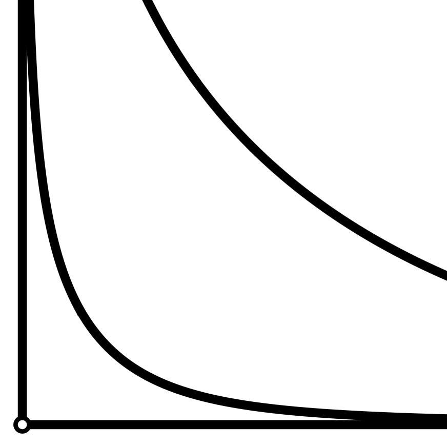
(a) Region I

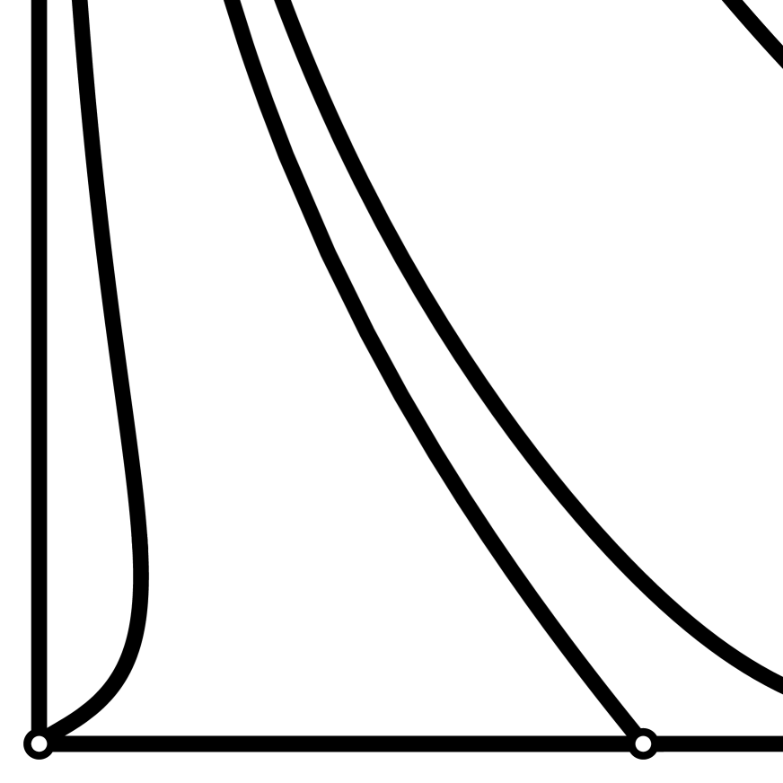
(b) Region II

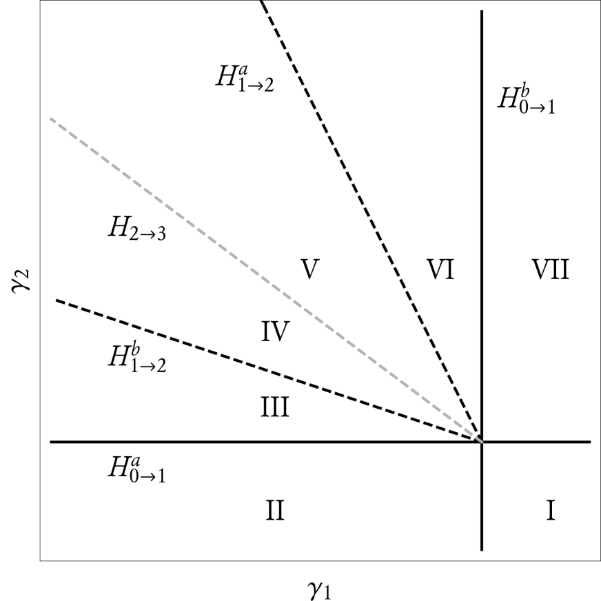
(c) Region III

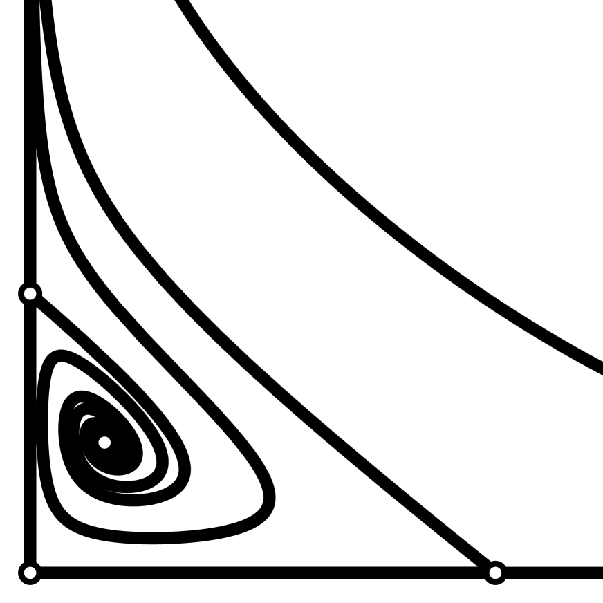
(d) Region IV

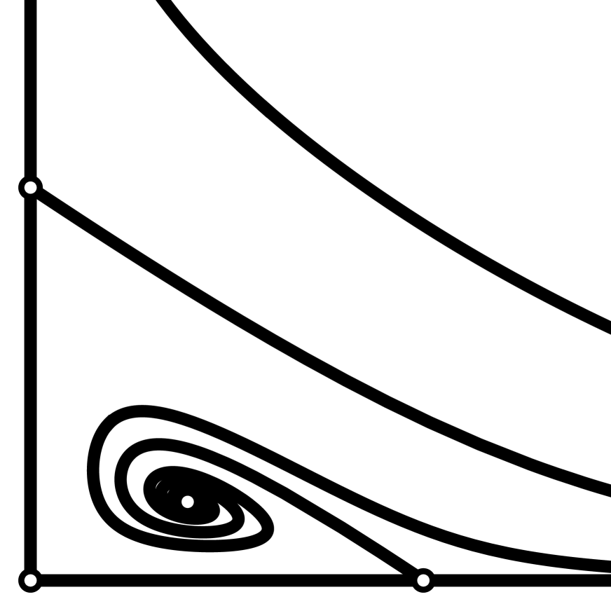
(e) Region V

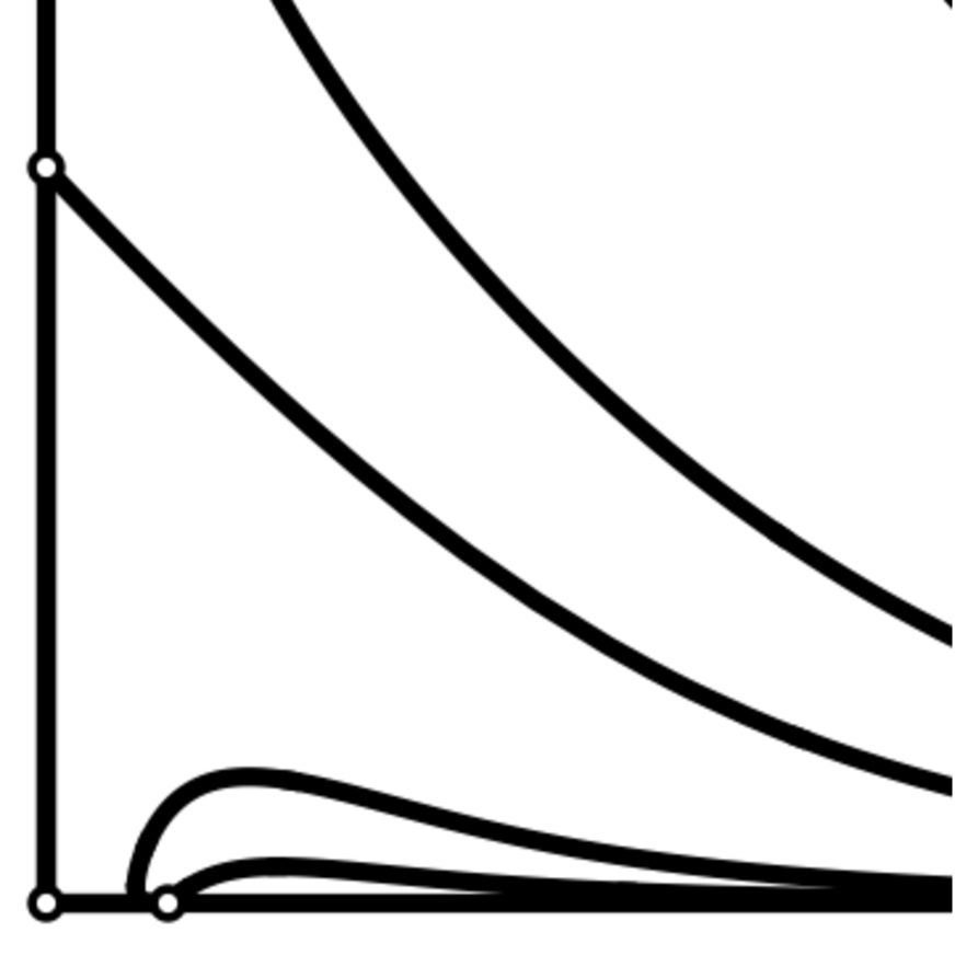
(f) Region VI

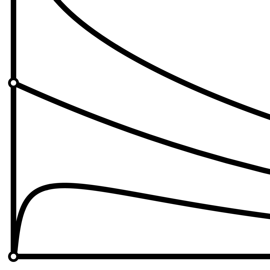
(g) Region VII

(h) $H_{2\to 3}$

Figure 1: Bifurcation diagram of (14) with $P=(^{2^{-1}}_{-1}{}^{\;\;3}_{-1})$. The parameters $\gamma_{1}$ and $\gamma_{2}$ are scaled versions of the real parts $\beta_{j}$ of the two pairs of eigenvalues. The regions I–VII in the central picture refer to the surrounding phase portraits on the basis $\mathscr{B}$. For the coding of the subordinate Hopf bifurcations see the main text.

The $1$–tori in $\mathbb{R}^{4}$ bifurcating off from the origin correspond to the boundary equilibria. These tori pass in turn through a secondary Hopf bifurcation. For the boundary equilibrium $\bar{\sigma}=(-\gamma_{1}/p_{11},0)$, which under our assumptions on $P$ exists if $\gamma_{1}>0$, we obtain

$$\dot{\sigma}\;\;=\;\;\begin{pmatrix}-\gamma_{1}&-\frac{p_{21}}{p_{11}}\gamma_{1}\\ 0&\gamma_{2}-\frac{p_{21}}{p_{11}}\gamma_{1}\end{pmatrix}(\sigma-\bar{\sigma})\;+\;O(\|\sigma-\bar{\sigma}\|^{2}).$$

Hence, this equilibrium changes from attractor to saddle at

$$H^{a}_{1\to 2}\quad:\quad p_{21}\gamma_{1}\;-\;p_{11}\gamma_{2}\;\;=\;\;0.$$

Similarly, the boundary equilibrium $\bar{\sigma}=(0,-\gamma_{2}/p_{22})$ changes from attractor to saddle at

$$H^{b}_{1\to 2}\quad:\quad p_{22}\gamma_{1}\;-\;p_{12}\gamma_{2}\;\;=\;\;0.$$

Linearising the flow at the interior equilibrium yields

$$\dot{\sigma}\;\;=\;\;\begin{pmatrix}p_{11}\bar{\sigma}_{1}&p_{12}\bar{\sigma}_{1}\\ p_{21}\bar{\sigma}_{2}&p_{22}\bar{\sigma}_{2}\end{pmatrix}(\sigma-\bar{\sigma})\;+\;O(\|\sigma-\bar{\sigma}\|^{2}).$$

The characteristic equation of the matrix on the right hand side is

$$0 \;\;=\;\;\det\begin{pmatrix}p_{11}\bar{\sigma}_{1}-\lambda&p_{12}\bar{\sigma}_{1}\\ p_{21}\bar{\sigma}_{2}&p_{22}\bar{\sigma}_{2}-\lambda\end{pmatrix}\;\;=\;\;\bar{\sigma}_{1}\bar{\sigma}_{2}\det\begin{pmatrix}p_{11}-\lambda/\bar{\sigma}_{1}&p_{12}\\ p_{21}\bar{\sigma}_{2}&p_{22}-\lambda/\bar{\sigma}_{2}\end{pmatrix}\enspace.$$

The equilibrium has imaginary eigenvalues if

$$\text{trace}\begin{pmatrix}p_{11}\bar{\sigma}_{1}&p_{12}\bar{\sigma}_{1}\\ p_{21}\bar{\sigma}_{2}&p_{22}\bar{\sigma}_{2}\end{pmatrix}\;\;=\;\;p_{11}\bar{\sigma}_{1}+p_{22}\bar{\sigma}_{2}\;\;=\;\;0$$

and

$$\det\begin{pmatrix}p_{11}\bar{\sigma}_{1}&p_{12}\bar{\sigma}_{1}\\ p_{21}\bar{\sigma}_{2}&p_{22}\bar{\sigma}_{2}\end{pmatrix}\;\;=\;\;(\det P)\bar{\sigma}_{1}\bar{\sigma}_{2}\;\;>\;\;0.$$

The first condition can only be satisfied if the signs of $p_{11}$ and $p_{22}$ are opposite, as we have assumed. The second condition is always satisfied given our assumption that $\det P>0$. The first condition can be written as

$$H_{2\to 3}\quad:\quad p_{22}(p_{21}-p_{11})\gamma_{1}\;+\;p_{11}(p_{12}-p_{22})\gamma_{2}\;\;=\;\;0.$$

It is well-known [25] that this Hopf bifurcation is degenerate, and that the base system has a first integral at the $H_{2\to 3}$ bifurcation value. Using the condition, the normal frequency at Hopf bifurcation can be expressed as a function of the scaled parameter $\gamma_{1}$ as

$$\sqrt{(\det P)\bar{\sigma}_{1}\bar{\sigma}_{2}}\;\;=\;\;|\gamma_{1}||p_{21}-p_{11}|\sqrt{(p_{12}p_{21}-p_{11}p_{22})p_{11}/p_{22}}$$

The location of the Hopf bifurcation curves is illustrated in figure 1.

4.4 Dynamics on the reduced phase space $\mathscr{P}$

Joining the fibre dynamics (14b) to the basis dynamics (14a), for $\varepsilon=0$ we find two degeneracies. First, for parameters at the $H_{2\to 3}$ Hopf bifurcation value, the basis dynamics has a first integral. Second, an equilibrium $\bar{\sigma}$ of the basis dynamics corresponds to a limit cycle as long as the frequency $\xi+\langle\ell^{\perp}\mid Q\bar{\sigma}\rangle$ does not vanish and to a circle of equilibria where it does vanish. In the latter case we speak of a resonance droplet.

Figure 2: The normal form (14) does not fully resolve the resonance droplet, which is shown as a grey segment. In the left hand picture we use the scaled eigenvalue parameters $\gamma_{1}$ and $\gamma_{2}$. In the right hand picture we replace $\gamma_{1}$ by the frequency $\xi,$ defined in (11). Also not resolved is the Hopf line $H_{2\to 3}$, which should yield a whole range of parameters with periodic orbits on the basis $\mathscr{B}$, which is also shown in grey.

Now consider (12) for $\varepsilon>0$. There are two situations, according to whether the frequency $\xi+\langle\ell^{\perp}\mid Q\bar{\sigma}\rangle$ of the fibre dynamics does or does not vanish. If $\bar{\sigma}$ is a hyperbolic equilibrium of the basis dynamics and if $\xi+\langle\ell^{\perp}\mid Q\bar{\sigma}\rangle$ does not vanish, the limit cycle $\{\bar{\sigma}\}\times\mathbb{T}$ survives a small perturbation. If $\bar{\sigma}$ is at the subordinate Hopf bifurcation $H_{2\to 3}$ we have to normalise to higher order than $4$ to resolve the degeneracy. As shown in [25] already one additional order suffices. This has consequences only for the low order $1{:}2$ and $1{:}3$ resonances where indeed $|\ell|\leq 4$. For the higher order resonances we already do normalise to order $|\ell|\geq 5$. Note that next to the Hopf line $H_{2\to 3}$ also the resonance bubbles are not fully resolved, see figure 2.

In this way the family of periodic orbits at a single parameter value gets re-distributed over a range of parameters, starting at the Hopf bifurcation $H_{2\to 3}$ and ending at the parameter value $\mathit{Het}$ of a heteroclinic bifurcation where a closed orbit disappears in a blue sky bifurcation.

4.5 Saddle-node bifurcations on the reduced phase space $\mathscr{P}$

We proceed to find the equilibria of (12), which satisfy the equations

$$0 \;\;=\;\;\gamma\;+\;P\sigma\;+\;\varepsilon^{2}\tilde{p}\;+\;\varepsilon^{|\ell|-2}A\psi,$$ (15a)

$$0 \;\;=\;\;\xi\;+\;\langle\ell^{\perp}\mid Q\sigma\;+\;\varepsilon^{2}\tilde{q}\;+\;\varepsilon^{|\ell|-2}B\psi\rangle,$$ (15b)

together with the syzygy (13).

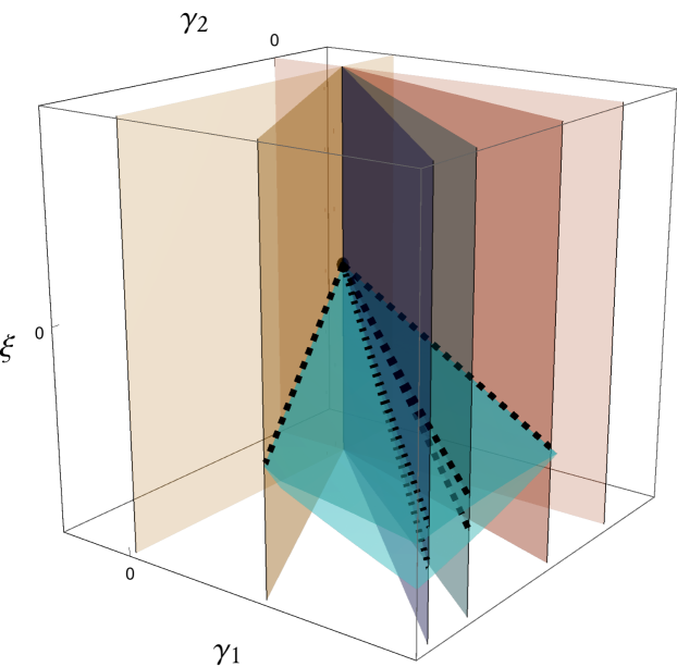
Figure 3: Local bifurcation diagram of the family (12) in the space of the scaled eigenvalue parameters $\gamma_{1}$, $\gamma_{2}$ and the frequency $\xi,$ defined in (11). The orange planes are the Hopf bifurcations taken over from figure 1. In green we furthermore include the saddle-node bifurcations originating from the resonance droplets in figure 2. Finally, the purple plane denotes the heteroclinic bifurcations, which originate from resolving the $H_{2\to 3}$ bifurcation.

As $P$ is invertible, which is the only situation we consider, equation (15a) can be solved in the form

$$\sigma\;\;=\;\;\Phi_{0}(\gamma,\varepsilon^{2})\;+\;\varepsilon^{|\ell|-2}\Phi_{1}(\gamma,\varepsilon^{2},\varepsilon^{|\ell|-2}A\psi)A\psi$$

where $\Phi_{0}(\gamma,0)=-P^{-1}\gamma$ and $\Phi_{1}(\gamma,0,0)=-P^{-1}$. Substitution into (15b) yields

$$0 \;\;=\;\;\xi\;+\;\langle\ell^{\perp}\mid Q\Phi_{0}+\varepsilon^{2}\tilde{q}\rangle\;+\;\varepsilon^{|\ell|-2}\langle\ell^{\perp}\mid(B+\Phi_{1}A)\psi\rangle.$$ (16)

To describe the saddle-node bifurcation curves, we perform a blow-up by introducing the scaled parameter $\zeta$ as

$$\varepsilon^{|\ell|-2}\zeta\;\;=\;\;\xi\;+\;\langle\ell^{\perp}\mid Q\Phi_{0}+\varepsilon^{2}\tilde{q}\rangle.$$

Dividing by $\varepsilon^{|\ell|-2}$, this transforms (16) into

$$0 \;\;=\;\;\zeta\;+\;\langle\ell^{\perp}\mid(B+\Phi_{1}A)\psi\rangle.$$ (17)

As an equation in $\psi$, (17) describes a family of curves that for $\varepsilon=0$ reduces to a family of lines, since $\Phi_{1}$, $A$ and $B$ are independent of $\psi$. For fixed values of $\sigma$, the syzygy (13) defines a circle. The curves (17) intersect the circle in either zero or two points, or they touch the circle. In the latter situation, we have a saddle-node bifurcation of equilibria, defining the boundaries of a resonance droplet of width $\varepsilon^{|\ell|-2}$. The resulting bifurcation diagram is given in figure 3.

(a) $1{:}2$ resonance

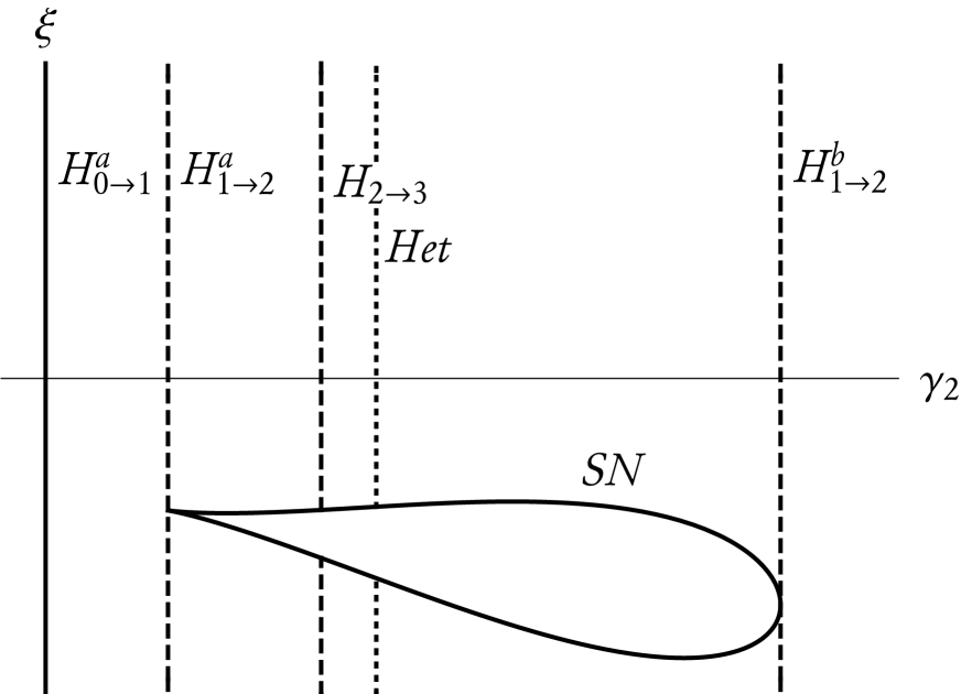
(b) $1{:}3$ resonance

(c) $1{:}4$ resonance

(d) $2{:}3$ resonance

Figure 4: Vertical sections of the bifurcation diagram given in figure 3. So we fix $\gamma_{1}$ and only consider the parameters $\gamma_{2}$ and $\xi$. Shape of the resonance droplets for the $1{:}2$, the $1{:}3$, the $1{:}4$ and the $2{:}3$ resonances.

Writing $R^{2}=\bar{\sigma}_{1}^{\ell_{2}}\bar{\sigma}_{2}^{\ell_{1}}/G_{\ell}$ and $m=(B-PA)^{T}\ell^{\perp}$, the condition that the line $\langle m\mid\psi\rangle+\zeta=0$ touches the circle $|\psi|=R$ implies that $\psi=\alpha m$ for a real scalar $\alpha$ that satisfies $|\alpha|=R/|m|$. For $\varepsilon=0$ the saddle-node bifurcation condition can then be written as

$$\zeta\;\;=\;\;\pm|m|R\;\;=\;\;\pm C\bar{\sigma}_{1}^{\ell_{2}/2}\bar{\sigma}_{2}^{\ell_{1}/2}.$$ (18)

Since a line is flat and a circle has constant curvature, it is clear that — for sufficiently small $\varepsilon>0$ — the saddle-node bifurcation is nondegenerate.

Equation (18) shows that the saddle-node curves are the boundaries of a resonance droplet with width proportional to $\bar{\sigma}_{1}^{\ell_{2}/2}$ close to the Hopf curve $\bar{\sigma}_{1}=0$ and width proportional to $\bar{\sigma}_{2}^{\ell_{1}/2}$ close to the Hopf curve $\bar{\sigma}_{2}=0$. This is illustrated in figures 4 and 5.

(a) $1{:}2$ resonance

(b) $1{:}3$ resonance

(c) $1{:}4$ resonance

(d) $2{:}3$ resonance

Figure 5: Horizontal sections of the bifurcation diagram given in figure 3. So we fix $\xi$ and only consider the parameters $\gamma_{1}$ and $\gamma_{2}$. Shape of the resonance droplets for the $1{:}2$, the $1{:}3$, the $1{:}4$ and the $2{:}3$ resonances.

4.6 Putting it all together

When the saddle-node bifurcation on the invariant circle coincides with the occurrence of two unit Floquet multipliers of the limit circle, we expect a fold-Hopf bifurcation to occur. In figures 4 and 5 these are the two points where the line $H_{2\to 3}$ — which ceases to exist inside the resonance droplet — meets the resonance droplet at the boundary.

5 Dynamics of the full system

In the previous section we analysed the dynamics of the truncated normal form on $\mathbb{R}^{4}$, i.e. after reduction of the $\mathbb{T}^{n}$ symmetry. Reconstructing the dynamics of the truncated normal form on $\mathbb{T}^{n}\times\mathbb{R}^{4}$ amounts to restoring the driving

$$\dot{x}\;\;=\;\;\omega(\mu)\;+\;\hat{f}(\tau_{1},\tau_{2},\mu)\;+\;a_{0}(\mu)\tau_{3}\;+\;c_{0}(\mu)\tau_{4},$$

which for $\tau=0$ is conditionally periodic with frequency vector $\omega(\mu)$. On $\mathbb{R}^{4}$ we still have a $\mathbb{T}$ symmetry in the resonant case and a $\mathbb{T}^{2}$ symmetry in the non-resonant case (or if we choose an order of truncation lower than the order $|\ell|$ of $\tau_{3}$ and $\tau_{4}$). Reducing the former takes us to the reduced phase space $\mathscr{P}$ and reducing the latter takes us directly to the basis $\mathscr{B}$ of the circle bundle $\mathscr{P}$.

For general survey in the relevant kam theory, see [10, 18, 14, 22]. The general philosophy is that we first are given a generic integrable (i.e. torus symmetric) system, where the dimension of the torus equals $n$, $n+1$ or $n+2$. The Diophantine conditions (9) determine a ‘Cantorised’ sub-bundle which is nowhere dense, but of large Lebesgue measure for small values of the gap parameter $\Gamma$. Restricted to this set a Whitney smooth conjugation exists with a subset of the perturbed system. This result is called quasi-periodic stability: structural stability restricted to a bundle of Diophantine quasi-periodic tori. The main question here is what happens in the gaps of this Cantorised bundle. In the present dissipative context hyperbolicity plays an important role in the perturbation analysis.

5.1 No resonance

The truncated normal form is not only independent of $x$ but also independent of $\tau_{3}$ and $\tau_{4}$ if there is no resonance (2) with $\ell\neq 0$ between the normal frequencies $\alpha_{1}(0)$ and $\alpha_{2}(0)$, or if we chose an order of truncation that is lower than the order $|\ell|$ of $\tau_{3}$ and $\tau_{4}$ in case there is a resonance $\ell\neq 0$ of the form (2). Reconstructing the dynamics on $\mathbb{R}^{4}$ from the reduced dynamics on $\mathscr{B}$ is already implicit in figure 1. Indeed, it is the reconstructed toral dynamics that turns the pitchfork bifurcations that are actually visible in that figure into the Hopf bifurcations $H^{a,b}_{0\to 1}$ and $H^{a,b}_{1\to 2}$. On $\mathbb{T}^{n}\times\mathbb{R}^{4}$ these then reconstruct to Hopf bifurcations of $n$–tori and $(n+1)$–tori, respectively, resulting in tori of dimensions $n+1$ and $n+2$.

For $n=0$ persistence of the latter — when perturbing from the normal form back to the original system — has been proved in [33], as has been persistence of the $3$–tori resulting from the quasi-periodic Hopf bifurcation $H_{2\to 3}$. Persistence of the three types of Hopf bifurcations of $n$–tori, $(n+1)$–tori and $(n+2)$–tori also follows from [3, 22], see furthermore [9]. We remark that the specialised approach in [33] yields the same order $\varepsilon^{1/18}$ as the general treatment in [3]. Indeed, in [3] we have a general normal form as in Theorem 3.1, where we have to go up to $8$th order. Accounting each normalisation step by $\sqrt{\varepsilon}$, the remainder terms turn out to be of order $\varepsilon^{1/18}$.

The gaps left open when Cantorising the attracting tori to prove persistence using kam theory can be closed using normal hyperbolicity to obtain invariant tori on which the flow is no longer quasi-periodic, compare with [8] and results cited therein. There seem to be no claims concerning the heteroclinic bifurcation in the literature.

5.2 Higher order resonances

Here we normalise op to order $|\ell|\geq 5$. This makes the $1{:}4$ and $2{:}3$ resonances still special among the higher order resonances as normalising up to $5$th order to resolve the Hopf bifurcation $H_{2\to 3}$ automatically includes $\tau_{3}$ and $\tau_{4}$ into the normal form. Note that the opening of the resonance bubbles is dictated by $\ell_{1}$ and $\ell_{2}$ separately, see e.g. figures 4c and 5c.

Where the line $H_{2\to 3}$ meets the resonance bubble we have a fold-Hopf bifurcation; in fact the line ceases to exist inside the resonance bubble. Next to the Hopf bifurcations $H^{a,b}_{0\to 1}$ of $n$–tori, for the persistence of which we again refer to [3, 22, 9], this leaves us with six special points: the two Hopf bifurcations $H^{a,b}_{1\to 2}$ of $(n+1)$–tori with a normal-internal resonance, the two fold-Hopf bifurcations and the two heteroclinic bifurcations at the boundary of the resonance bubble (which we do not further comment upon).

5.3 The $1{:}3$ resonance

In this case $|\ell|-2=2$, which means that we have two competing influences in the normal form. Hence, the relative strengths of the coefficients $\tilde{p}$ and $A\psi$ in (12) decides whether we have dynamics similar to the previous subsection or dynamics similar to the following subsection.

5.4 The $1{:}2$ resonance

Although the invariants $\tau_{3}$ and $\tau_{4}$ have order $|\ell|=3$ in this case, we still work with a $5$th order normal form to resolve the Hopf bifurcation $H_{2\to 3}$. In this way not only the linear terms $\tau_{3}$ and $\tau_{4}$ enter the normal form, but also the four $5$th order terms $\tau_{i}\tau_{j}$ with $i=1,2$ and $j=3,4$. We wonder whether the subordinate fold-Hopf bifurcation requests even higher order terms of the normal form or whether the $5$th order terms are already sufficient, again see [9].

At the end points of the resonance bubble we have periodic Hopf bifurcations $H^{a,b}_{1\to 2}$ with normal-internal resonances $1{:}1$ and $1{:}2$, respectively.

6 Final remarks

The $\mathbb{T}^{1}$ or $\mathbb{T}^{2}$ symmetric normal form analysis forms a kind of skeleton of the total dynamics, which occurs when adding the non-symmetric, higher order terms that are flat.

First note that normal forms of any finite order keep the toroidal symmetry. That means that flat terms are of infinite order and we expect these terms to be exponentially small in the real analytic context [17, 13, 8]. In the present dissipative context the higher order resonances in the Diophantine conditions (9) give rise to infinite arrays of ‘small’ resonance bubbles [4, 2, 3, 8, 9, 19, 20, 21], where the array ‘runs along’ the bifurcation manifolds as given by the quasi-periodic sub-bundle, compare with the discussion at the beginning of section 5. The paper [8] exactly uses the quasi-periodic Hopf bifurcation as a leading example.

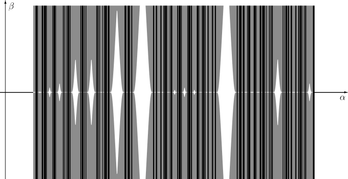
Figure 6: From [8]. Parameter sets with persistent invariant tori and the subset of persistent quasi-periodic invariant tori. The latter (black) set is the product of a Cantor set in the $\alpha$–direction and the real line in the $\beta$–direction: it is nowhere dense. The (white) complement of the former set (which includes the resonance set on the $\beta$–axis) is a ‘set of ignorance’.

Inside the bubbles the complexity is large both in the dissipative and conservative context, which is illustrated by the papers [15, 16, 43].

References

- [1] V.I. Arnol’d, On matrices depending on parameters. Russian Mathematical Surveys 26:2 (1971) 29–43
- [2] B.L.J. Braaksma and H.W. Broer, On a quasi-periodic Hopf bifurcation. Annales Institut Henri Poincaré, Analyse non linéaire 4 (1987) 115–168
- [3] B.L.J. Braaksma, H.W. Broer and G.B. Huitema, Towards a quasi-periodic bifurcation theory. Memoirs American Mathematical Society 83 # 421 (1990) 83–167
- [4] H.W. Broer, Coupled Hopf-bifurcations: Persistent examples of –quasiperiodicity given by families of 3-jets. Astérisque 286 (2003) 223–229
- [5] H.W. Broer, R. van Dijk and Re. Vitolo, Survey of strong normal-internal resonances in quasi-periodically driven oscillators for In G. Gaeta, Ra. Vitolo and S. Walcher (eds.), Symmetry and Perturbation Theory, Proceedings of the International Conference SPT 2007. World Scientific (2007) 45–55
- [6] H.W. Broer, H. Hanßmann and J. Hoo, The quasi-periodic Hamiltonian Hopf bifurcation. Nonlinearity 20 (2007) 417–460
- [7] H.W. Broer, H. Hanßmann, À. Jorba, J. Villanueva and F.O.O. Wagener, Normal-internal resonances in quasi-periodically forced oscillators: a conservative approach. Nonlinearity 16 (2003) 1751–1791
- [8] H.W. Broer, H. Hanßmann and F.O.O. Wagener, Persistence Properties of Normally Hyperbolic Tori. Regular and Chaotic Dynamics 23 (2018) 212–225
- [9] H.W. Broer, H. Hanßmann and F.O.O. Wagener, Quasi-Periodic Bifurcation Theory, the geometry of KAM. Springer, in preparation
- [10] H.W. Broer, G.B. Huitema and M.B. Sevryuk, Quasi-Periodic Motions in Families of Dynamical Systems: Order amidst Chaos. Lecture Notes in Mathematics 1645, Springer (1996)
- [11] H.W. Broer, G.B. Huitema and F. Takens, Unfoldings of quasi-periodic tori. Memoirs American Mathematical Society 83 # 421 (1990) 1–81
- [12] H.W. Broer, V. Naudot, R. Roussarie, K. Saleh and F.O.O. Wagener, Organising centres in the semi-global analysis of dynamical systems. Int. J. Appl. Math. Stat. 12(D07) (2007) 7–36
- [13] H.W. Broer and R. Roussarie, Exponential confinement of chaos in the bifurcation set of real analytic diffeomorphisms. In: H.W. Broer, B. Krauskopf and G. Vegter (eds.) Global Analysis of Dynamical Systems, Leiden 2001. Festschrift dedicated to Floris Takens for his 60th birthday. Inst. of Phys. (2001) 167–210
- [14] H.W. Broer and M.B. Sevryuk, kam Theory: quasi-periodicity in dynamical systems. In: H.W. Broer, B. Hasselblatt, F. Takens (eds.) Handbook of Dynamical Systems 3 North-Holland (2010)
- [15] H.W. Broer, C. Simó and R. Vitolo, The Hopf-Saddle-Node bifurcation for fixed points of 3D-diffeomorphisms, analysis of a resonance ‘bubble’, Physica D 237 (2008), 1773–1799
- [16] H.W. Broer, C. Simó and R. Vitolo, The Hopf-Saddle-Node bifurcation for fixed points of 3D-diffeomorphisms: the Arnol’d resonance web, Bull. Belgian Math. Soc. Simon Stevin 15 (2008), 769–787
- [17] H.W. Broer and F. Takens, Formally symmetric normal forms and genericity. Dynamics Reported 2 (1989) 36–60
- [18] H.W. Broer and F. Takens, Dynamical Systems and Chaos. Epsilon Uitgaven 64 (2009); Applied Mathematical Sciences 172, Springer (2011)
- [19] A. Chenciner, Bifurcations des points elliptiques-I. Courbes invariantes. Publications Mathématiques Institut Hautes Études 61 (1985) 67–127
- [20] A. Chenciner, Bifurcations des points elliptiques-II. Orbites périodiques et ensembles de Cantor invariants. Inventiones Mathematicæ 80 (1985) 81–106
- [21] A. Chenciner, Bifurcations des points elliptiques-III. Orbites périodiques de “petites” périodes et élimination résonnante des couples de courbes invariantes. Publications Mathématiques Institut Hautes Études 66 (1987) 5–91.
- [22] M.C. Ciocci, A. Litvak-Hinenzon and H.W. Broer, Survey on dissipative KAM theory including quasi-periodic bifurcation theory. In: J. Montaldi and T.S. Raţiu (eds.) Geometric Mechanics and Symmetry: the Peyresq Lectures. Cambridge University Press (2005) 303–355
- [23] S.A. van Gils, M. Krupa and W.F. Langford, Hopf bifurcation with non-semisimple 1:1 resonance. Nonlinearity 3 (1990) 825–850
- [24] M. Golubitsky and M. Krupa, Stability computations for nilpotent Hopf bifurcations in coupled cell systems. Int. J. Bifurcation Chaos 17 (2007) 2595–2603
- [25] J. Guckenheimer and P. Holmes, Nonlinear Oscillations, Dynamical Systems, and Bifurcations of Vector Fields, Fifth Edition. Applied Mathematical Sciences 42, Springer (1997)
- [26] H. Hanßmann, Local and Semi-Local Bifurcations in Hamiltonian Dynamical Systems — Results and Examples. Lecture Notes in Mathematics 1893, Springer (2007)
- [27] F. Hausdorff, Set Theory. Chelsea (1962) [German original: Veit (1914)]
- [28] E. Knobloch and M.R.E. Proctor, The double Hopf bifurcation with 2:1 resonance. Proc. R. Soc. London A415 (1988) 61–90
- [29] A.M. Krasnosel\cprimeskii, D.I Rachinskii and K. Schneider, Hopf bifurcations in resonance . Nonlinear Analysis 52 (2003) 943–960
- [30] Yu. Kuznetsov, Elements of applied bifurcation theory. Applied Mathematical Sciences 112, Springer (1995)
- [31] V.G. LeBlanc, On some secondary bifurcations near resonant Hopf-Hopf interactions. Dyn. Contin. Discr. Imp. Syst.: Ser. B: App. Algorithms 7 (2000) 405–427
- [32] V. LeBlanc and W.F. Langford, Classifications and unfoldings of 1:2 resonant Hopf bifurcation. Arch. Rational Mech. Anal. 136 (1996) 305–357
- [33] X. Li, On the persistence of quasi-periodic invariant tori for double Hopf bifurcation of vector fields. Journal of Differential Equations 260 (2016) 7320–7357
- [34] A. Luongo, A. Paolone and A. Di Egidio, Multiple timescales analysis for 1:2 and 1:3 resonant Hopf bifurcations. Nonlinear Dyn. 34 (2003) 269–291
- [35] J.K. Moser, Convergent Series Expansion for Quasi-Periodic Motions. Mathematische Annalen 169 (1967) 136–176
- [36] N.S. Namachchivaya, M.M. Doyle, W.F. Langford and N.W. Evans, Normal form for generalized Hopf bifurcation with non-semisimple 1:1 resonance. Z. Angew. Math. Phys. 45 (1994) 312–335
- [37] G. Revel, D.M. Alonso and J.L. Moiola, Interactions between oscillatory modes near a 2:3 resonant Hopf-Hopf bifurcation. Chaos 20 (2010) 043106
- [38] G. Revel, D.M. Alonso and J.L. Moiola, Numerical semi-global analysis of a 1:2 resonant Hopf-Hopf bifurcation. Physica D 247 (2013) 40–53
- [39] G. Revel, D.M. Alonso and J.L. Moiola, A Degenerate 2:3 Resonant Hopf-Hopf Bifurcation as Organizing Center of the Dynamics: Numerical Semiglobal Results. SIAM J. Appl. Dyn. Sys. 14 (2015) 1130–1164
- [40] K. Saleh and F.O.O. Wagener, Semi-global analysis of periodic and quasi-periodic normal-internal and resonances. Nonlinearity 23 (2010) 2219–2252
- [41] P.H. Steen and S.H. Davis, Quasiperiodic bifurcation in nonlinearly-coupled oscillators near a point of strong resonance. SIAM J. Appl. Math. 42 (1982) 1345–1368
- [42] F. Takens, Introduction to Global Analysis. Communications 2 of the Mathematical Institute, Rijksuniversiteit Utrecht (1973)
- [43] R. Vitolo, H.W. Broer and C. Simó, Routes to chaos in the Hopf-Saddle-Node bifurcation for fixed points of 3D-diffeomorphisms, Nonlinearity 23 (2010), 1919–1947
- [44] D.Yu. Volkov, The Andronov–Hopf bifurcation with 2:1 resonance. Journal of Mathematical Sciences 128 (2005) 2831–2834
- [45] F.O.O. Wagener, A note on Gevrey regular KAM theory and the inverse approximation lemma. Dynamical Systems 18 (2003) 159–163
- [46] F.O.O. Wagener, A parametrised version of Moser’s modifying terms theorem. In: H.W. Broer, H. Hanßmann and M.B. Sevryuk (eds.) KAM theory and its applications, Leiden 2008. Discrete Continuous Dynamical Systems, Ser.S 3 (2010) 719–768