Flexible models for overdispersed and underdispersed count data

Abstract

Within the framework of probability models for overdispersed count data, we propose the generalized fractional Poisson distribution (gfPd), which is a natural generalization of the fractional Poisson distribution (fPd), and the standard Poisson distribution. We derive some properties of gfPd and more specifically we study moments, limiting behavior and other features of fPd. The skewness suggests that fPd can be left-skewed, right-skewed or symmetric; this makes the model flexible and appealing in practice. We apply the model to real big count data and estimate the model parameters using maximum likelihood. Then, we turn to the very general class of weighted Poisson distributions (WPD’s) to allow both overdispersion and underdispersion. Similarly to Kemp’s generalized hypergeometric probability distribution, which is based on hypergeometric functions, we analyze a class of WPD’s related to a generalization of Mittag–Leffler functions. The proposed class of distributions includes the well-known COM-Poisson and the hyper-Poisson models. We characterize conditions on the parameters allowing for overdispersion and underdispersion, and analyze two special cases of interest which have not yet appeared in the literature.

Keywords: Left-skewed, Big count data, underdispersion, overdispersion, COM-Poisson, Hyper-Poisson, Weighted Poisson, Fractional Poisson distribution

1 Introduction and mathematical background

The negative binomial distribution is one of the most widely used discrete probability models that allow departure from the mean-equal-variance Poisson model. More specifically, the negative binomial distribution models overdispersion of data relative to the Poisson distribution. For clarity, we refer to the extended negative binomial distribution with probability mass function

$$P(X=x)=\frac{\Gamma(r+x)}{\Gamma(r)x!}p^{r}(1-p)^{x},\qquad x=0,1,2,\ldots,$$ (1)

where $r>0$. If $r\in\{1,2,\dots\}$, $x$ is the number of failures which occur in a sequence of independent Bernoulli trials to obtain $r$ successes, and $p$ is the success probability of each trial.

One limitation of the negative binomial distribution in fitting overdispersed count data is that the skewness and kurtosis are always positive. An example is given in Section 2.1.1, in which we introduce two real world data sets that do not fit a negative binomial model. The data sets reflect reported incidents of crime that occurred in the city of Chicago from January 1, 2001 to May 21, 2018. These data sets are overdispersed but the skewness coefficients are estimated to be respectively -0.758 and -0.996. Undoubtedly, the negative binomial model is expected to underperform in these types of count populations. These data sets are just two examples in a yet to be discovered non-negative binomial world, thus demonstrating the real need for a more flexible alternative for overdispersed count data. The literature on alternative probabilistic models for overdispersed count data is vast. A history of the overdispersed data problem and related literature can be found in [32]. In this paper we consider the fractional Poisson distribution (fPd) as an alternative. The fPd arises naturally from the widely studied fractional Poisson process [31, 33, 15, 21, 3, 5, 25]. It has not yet been studied in depth and has not been applied to model real count data. We show that the fPd allows big (large mean), both left- and right-skewed overdispersed count data making it attractive for practical settings, especially now that data are becoming more available and bigger than before. fPd’s usually involve one parameter; generalizations to two parameters are proposed in [3, 13]. Here, we take a step forward and further generalize the fPd to a three parameter model, proving the resulting distribution is still overdispersed.

One of the most popular measures to detect the departures from the Poisson distribution is the so-called Fisher index which is the ratio of the variance to the mean $(\lessgtr 1)$ of the count distribution. As shown in the crime example of Section 2.1.1, the computation of the Fisher index is not sufficient to determine a first fitting assessment of the model, which indeed should take into account at least the presence of negative/positive skewness. To compute all these measures, the first three factorial moments should be considered. Consider a discrete random variable $X$ with probability generating function (pgf)

$$G_{X}(u)=\bm{E}u^{X}=\sum_{k\geq 0}a_{k}\frac{(u-1)^{k}}{k!},\qquad|u|\leq 1,$$ (2)

where $\{a_{k}\}$ is a sequence of real numbers such that $a_{0}=1.$ Observe that $Q(t)=G_{X}(1+t)$ is the factorial moment generating function of $X.$ The $k$-th moment is

$$\bm{E}X^{k}=\sum_{r=1}^{k}S(k,r)a_{r},$$ (3)

where $S(k,r)$ are the Stirling numbers of the second kind [11]. By means of the factorial moments it is straightforward to characterize overdispersion or underdispersion as follows: letting $a_{2}>a_{1}^{2}$ yields overdispersion whereas $a_{2}<a_{1}^{2}$ gives underdispersion. Let $c_{2}$ and $c_{3}$ be the second and third cumulant of $X$, respectively. Then, the skewness can be expressed as

$$\gamma(X)=\frac{c_{3}}{c_{2}^{3/2}}=\frac{a_{3}+3a_{2}+a_{1}[1-3a_{2}+a_{1}(2a_{1}-3)]}{(a_{1}+a_{2}-a_{1}^{2})^{3/2}}.$$ (4)

If the condition

$$\lim_{n\rightarrow\infty}\frac{a_{n}}{(n-k)!}=0,\qquad k\leq n,$$ (5)

is fulfilled, the probability mass function of $X$ can be written in terms of its factorial moments [9]:

$$P(X=x)=\frac{1}{x!}\sum_{k\geq 0}a_{k+x}\frac{(-1)^{k}}{k!},\qquad x\geq 0.$$ (6)

As an example, the very well-known generalized Poisson distribution which accounts for both under and overdispersion [23, 7], put in the above form has factorial moments given by $a_{0}=1$ and

$$a_{k}=\sum_{r=0}^{h(\lambda_{2})}\frac{1}{r!}\lambda_{1}(\lambda_{1}+\lambda_{2}(r+k))^{r+k-1}e^{-(\lambda_{1}+\lambda_{2}(r+k))},\qquad\lambda_{1}>0,$$ (7)

where $h(\lambda_{2})=\infty$ and $k=1,2,\ldots$, if $\lambda_{2}>0$. While $h(\lambda_{2})=M-k$ and $k=1,\ldots,M$, if $\max(-1,-\lambda_{1}/M)\leq\lambda_{2}<0$ and $M$ is the largest positive integer for which $\lambda_{1}+M\lambda_{2}>0$.

Another example is given by the Kemp family of generalized hypergeometric factorial moments distributions (GHFD) [18] for which the factorial moments are given by

$$a_{k}=\frac{\Gamma\left[(a+k);(b+k)\right]\lambda^{k}}{\Gamma\left[(a);(b)\right]},\qquad k\geq 0,$$ (8)

where $\Gamma\left[(a);(b)\right]=\prod_{i=1}^{p}\Gamma(a_{i})/\prod_{j=1}^{q}\Gamma(b_{j})$, with $a_{1},\ldots,a_{p},b_{1},\ldots,b_{q}\in{\mathbb{R}}$ and $p,q$ non negative integers. The factorial moment generating function is $Q(t)=\,_{p}F_{q}\left[(a);(b);\lambda t\right]$, where

$${}_{p}F_{q}\left[(a);(b);z\right]=\,_{p}F_{q}(a_{1},\ldots,a_{p};b_{1},\ldots,b_{q};z)=\sum_{m\geq 0}\frac{(a_{1})_{m}\cdots(a_{p})_{m}}{(b_{1})_{m}\cdots(b_{q})_{m}}\frac{z^{m}}{m!},$$ (9)

and $(a)_{m}=a(a+1)\cdots(a+m-1),m\geq 1.$ Both overdispersion and underdispersion are possible, depending on the values of the parameters [37]. The generalized fractional Poisson distribution (gfPd), which we introduce in the next section, lies in the same class of the Kemp’s GHFD but with the hypergeometric function in (9) substituted by a generalized Mittag–Leffler function (also known as three-parameter Mittag–Leffler function or Prabhakar function). In this case, as we have anticipated above, the model is capable of not only describing overdispersion but also having a degree of flexibility in dealing with skewness.

It is worthy to note that there exists a second family of Kemp’s distributions, still based on hypergeometric functions and still allowing both underdispersion and overdispersion. This is known the Kemp’s generalized hypergeometric probability distribution (GHPD) [17] and it is actually a special case of the very general class of weighted Poisson distributions (WPD). Taking into account the above features, we thus analyze the whole class of WPD’s with respect to the possibility of obtaining under and overdispersion. In Theorem 3.2 we first give a general necessary and sufficient condition to have an underdispersed or an overdispersed WPD random variable in the case in which the weight function may depend on the underlying Poisson parameter $\lambda$. Special cases of WPD’s admitting a small number of parameters have already proven to be of practical interest, such as for instance the well-known COM-Poisson [8] or the hyper-Poisson [2] models. Here we present a novel WPD family related to a generalization of Mittag-Leffler functions in which the weight function is based on a ratio of gamma functions. The proposed distribution family includes the above-mentioned well-known classical cases. We characterize conditions on the parameters allowing overdispersion and underdispersion and analyze two further special cases of interest which have not yet appeared in the literature. We derive recursions to generate probability mass functions (and thus random numbers) and show how to approximate the mean and the variance.

The paper is organized as follows: in Section 2, we introduce the generalized fractional Poisson distribution, discuss some properties and recover the classical fPd as a special case. These models are fit to the two real-world data sets mentioned above. Section 3 is devoted to weighted Poisson distributions, their characteristic factorial moments and the related conditions to obtain overdispersion and underdispersion. Furthermore, the novel WPD based on a generalization of Mittag–Leffler functions is introduced and described in Section 3.1: we discuss some properties and show how to get exact formulae for factorial moments by using Faà di Bruno’s formula [34]. Two special models are then characterized depending on the values of the parameters and compared to classical models. Finally, some illustrative plots end the paper.

2 Generalized fractional Poisson distribution (gfPd)

Definition 2.1.

A random variable $X_{\alpha,\beta}^{\delta}\;\stackrel{{\scriptstyle d}}{{=}}\;$gfPd$(\alpha,\beta,\delta,\mu)$ if

$$P(X_{\alpha,\beta}^{\delta}=x)=\frac{\Gamma(\delta+x)}{x!\Gamma(\delta)}\mu^{x}\Gamma(\beta)E_{\alpha,\alpha x+\beta}^{\delta+x}(-\mu),\quad\mu>0;\,x\in\mathbb{N};\,\alpha,\beta\in(0,\;1];\,\delta\in(0,\;\beta/\alpha],$$ (10)

where

$$E_{\eta,\nu}^{\tau}(w)=\sum_{j=0}^{\infty}\frac{(\tau)_{j}}{j!\Gamma(\eta j+\nu)}\;w^{j},$$ (11)

$w\in\mathbb{C};\Re(\eta),\Re(\nu),\Re(\tau)>0$, is the generalized Mittag–Leffler function [29] and $(\tau)_{j}=\Gamma(\tau+j)/\Gamma(\tau)$ denotes the Pochhammer symbol.

To show non-negativity, notice that

$$\frac{\Gamma(\delta+x)}{\Gamma(\delta)}E_{\alpha,\alpha x+\beta}^{\delta+x}(-\mu)\geq 0\iff(-1)^{x}\frac{d^{x}}{d\mu^{x}}E_{\alpha,\beta}^{\delta}(-\mu)\geq 0,$$ (12)

that is, $E_{\alpha,\beta}^{\delta}(-\mu)$ is completely monotone. From [10], it is known that $E_{\alpha,\beta}^{\delta}(-\mu)$ is completely monotone if $\alpha,\beta\in(0,\;1],\delta\in(0,\;\beta/\alpha]$ and thus the pmf in (10) is non-negative.

Note that the probability mass function can be determined using the following integral representation [27]:

$$P(X_{\alpha,\beta}^{\delta}=x)=\frac{\Gamma(\beta)}{x!\Gamma(\delta)}\mu^{x}\int_{\mathbb{R}^{+}}e^{-\mu y}y^{\delta+x-1}\phi(-{\alpha},\beta-\alpha\delta;-y)dy,$$ (13)

where the Wright function $\phi$ is defined as the convergent sum [19]

$$\phi(\xi,\omega;z)=\sum\limits_{r=0}^{\infty}\frac{z^{r}}{r!\Gamma[\xi r+\omega]},\qquad\xi>-1,\omega,z\in{\mathbb{R}}.$$ (14)

Remark 2.1.

The random variable $X_{\alpha,\beta}^{\delta}$ has factorial moments

$$a_{k}=\frac{\Gamma(\beta)\Gamma(\delta+k)}{\Gamma(\alpha k+\beta)\Gamma(\delta)}\mu^{k},\qquad k\geq 0.$$ (15)

Hence the pgf is $G_{X_{\alpha,\beta}^{\delta}}(u)=\Gamma(\beta)E_{\alpha,\beta}^{\delta}(\mu(u-1))$, $|u|\leq 1$.

By expressing the moments in terms of factorial moments and after some algebra we obtain

$$\bm{E}[X_{\alpha,\beta}^{\delta}] =\frac{\Gamma(\beta)\delta\mu}{\Gamma(\beta+\alpha)},$$ (16)

$$\bm{V}\text{{ar}}[X_{\alpha,\beta}^{\delta}] =\frac{\Gamma(\beta)\delta\mu}{\Gamma(\beta+\alpha)}+\Gamma(\beta)\delta\mu^{2}\left(\frac{(\delta+1)}{\Gamma(\beta+2\alpha)}-\frac{\Gamma(\beta)\delta}{\Gamma(\beta+\alpha)^{2}}\right).$$ (17)

Theorem 2.1.

$X_{\alpha,\beta}^{\delta}$ exhibits overdispersion.

Proof.

We have

$$a_{2}>a_{1}^{2}\Leftrightarrow\frac{\delta+1}{\Gamma(2\alpha+\beta)}>\frac{\delta\Gamma(\beta)}{\Gamma^{2}(\alpha+\beta)}\Leftrightarrow\delta\bigg{(}\frac{\Gamma(\beta)}{\Gamma^{2}(\alpha+\beta)}-\frac{1}{\Gamma(2\alpha+\beta)}\bigg{)}<\frac{1}{\Gamma(2\alpha+\beta)}$$ (18)

and

$$\frac{\Gamma(\beta)}{\Gamma^{2}(\alpha+\beta)}-\frac{1}{\Gamma(2\alpha+\beta)}>0\quad{\rm as}\quad\text{Beta}(\beta,\alpha)>\text{Beta}(\alpha+\beta,\alpha).$$ (19)

Thus, the distribution is overdispersed for

$$\delta<\frac{\text{Beta}(\alpha+\beta,\alpha)}{\text{Beta}(\beta,\alpha)-\text{Beta}(\alpha+\beta,\alpha)}.$$ (20)

Observe that the function $\beta\text{Beta}(\beta,\alpha)$ is increasing in $\beta$ for $\alpha,\beta\in(0,1)$ as

$$\frac{\partial}{\partial\beta}\beta\text{Beta}(\beta,\alpha)=\text{Beta}(\beta,\alpha)(1+\beta(\psi(\beta)-\psi(\alpha+\beta))>0,$$ (21)

where $\psi$ is the digamma function. Note that (21) is positive by formula (1.3.3) of [22] as $\psi$ is increasing on $(0,\infty)$. Thus

$$\beta\text{Beta}(\beta,\alpha)<(\alpha+\beta)\text{Beta}(\alpha+\beta,\alpha)\Leftrightarrow\frac{\beta}{\alpha}<\frac{\text{Beta}(\alpha+\beta,\alpha)}{\text{Beta}(\beta,\alpha)-\text{Beta}(\alpha+\beta,\alpha)}$$ (22)

and for $\delta\in(0,\beta/\alpha)$ the bound (20) is always verified. ∎

2.1 Fractional Poisson distribution

This section analyzes the classical fPd, which is a special case of gfPd, and is obtained when $\beta=\delta=1$. The fPd can model asymmetric (both left-skewed and right-skewed) overdispersed count data for all mean count values (small and large). The fPd has probability mass function (pmf)

$$P(X_{\alpha}=x)=\mu^{x}E_{\alpha,\alpha x+1}^{x+1}(-\mu),\qquad x=0,1,2,\ldots,$$ (23)

where $\mu>0$, $\alpha\in[0,1]$.

Notice that if $\alpha=1$, the standard Poisson distribution is retrieved, while for $\alpha=0$ we have $X_{0}\stackrel{{\scriptstyle d}}{{=}}\text{Geo}\left(1/(1+\mu)\right)$. Indeed,

$$P(X_{0}=x)=\frac{\mu^{x}}{x!}\sum_{j=0}^{\infty}\frac{(j+x)!}{j!}(-\mu)^{j}=\frac{1}{1+\mu}\left(\frac{\mu}{1+\mu}\right)^{x},\qquad x\geq 0.$$ (24)

Furthermore, the probability mass function can be determined using the following integral representation [4]:

$$P(X_{\alpha}=x)=\frac{\mu^{x}}{x!}\int_{\mathbb{R}^{+}}e^{-\mu y}y^{x}M_{\alpha}(y)dy,$$ (25)

where the $M$-Wright function [24]

$$M_{\alpha}(y)=\sum\limits_{j=0}^{\infty}\frac{(-y)^{j}}{j!\Gamma[-\alpha j+(1-\alpha)]}=\frac{1}{\pi}\sum\limits_{j=1}^{\infty}\frac{(-y)^{j-1}}{(j-1)!}\Gamma(\alpha j)\sin(\pi\alpha j)$$ (26)

is the probability density function of the random variable $S^{-\alpha}$ with $S\stackrel{{\scriptstyle d}}{{=}}\alpha^{+}$-stable supported in $\mathbb{R}^{+}.$ By using (25), the cumulative distribution function turns out to be

$$F_{X_{\alpha}}(x)=\sum_{r=0}^{\infty}\binom{x+r-1}{x}\frac{(-1)^{r}\mu^{-(r+1)}}{\Gamma(1-\alpha(r+1))}{\mathbb{1}}_{(x>0)}(x).$$ (27)

Remark 2.2.

From (2.1), the random variable $X_{\alpha}$ has factorial moments

$$a_{k}=\frac{\mu^{k}k!}{\Gamma(1+\alpha k)},\qquad k\geq 0.$$ (28)

Hence the probability generating function is $G_{X_{\alpha}}(u)=E_{\alpha,1}^{1}\left(\mu\left(u-1\right)\right)$, $|u|\leq 1$.

With respect to the symmetry structure of $X_{\alpha}$, from (4) and (28), the skewness of $X_{\alpha}$ reads

$$\gamma(X_{\alpha})=\frac{\frac{1}{\mu^{2}\Gamma(1+\alpha)}+\frac{6}{\mu\Gamma(1+2\alpha)}+\frac{6}{\Gamma(1+3\alpha)}-\frac{3}{\mu\left[\Gamma(1+\alpha)\right]^{2}}-\frac{6}{\Gamma(1+\alpha)\Gamma(1+2\alpha)}+\frac{2}{[\Gamma(1+\alpha)]^{3}}}{\left(\frac{1}{\mu\Gamma(1+\alpha)}+\frac{2}{\Gamma(1+2\alpha)}-\frac{1}{[\Gamma(1+\alpha)]^{2}}\right)^{3/2}}.$$ (29)

Moreover,

$$\lim_{\mu\to\infty}\gamma(X_{\alpha})=\frac{\frac{6}{\Gamma(1+3\alpha)}-\frac{6}{\Gamma(1+\alpha)\Gamma(1+2\alpha)}+\frac{2}{\left[\Gamma(1+\alpha)\right]^{3}}}{\left(\frac{2}{\Gamma(1+2\alpha)}-\frac{1}{[\Gamma(1+\alpha)]^{2}}\right)^{3/2}}\neq 0,$$ (30)

which correctly vanishes if $\alpha=1$, like the ordinary Poisson distribution.

2.1.1 Simulation and parameter estimation

The integral representation (25) allows visualization of the probability mass function of $X_{\alpha}$ (see Figure 1). Figure 1 shows the flexibility of the fPd. The probability distribution ranges from zero-inflated right-skewed ($\alpha\to 0$) to left-skewed ($\alpha\to 1$) and symmetric ($\alpha=1$) overdispersed count data.

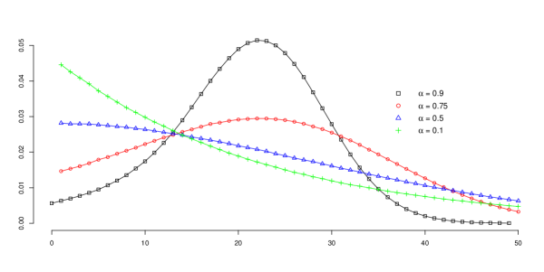
Figure 1: Probability mass functions of $X_{\alpha}$ for $\alpha=0.1,0.5,0.75,0.9$, and $\mu=20$.

To compute the integral in (25) by means of Monte Carlo techniques, we use the approximation,

$$p_{x}^{\alpha}\approx\frac{\mu^{x}}{\;x!}\left(\frac{1}{N}\sum_{j=1}^{N}e^{-\mu Y_{j}}Y_{j}^{x}\right),$$ (31)

where $Y_{j}^{\prime}s\;\stackrel{{\scriptstyle iid}}{{=}}S^{-\alpha}.$ Note that the random variable $S$ can be generated using the following formula [16, 6]:

$$S\stackrel{{\scriptstyle d}}{{=}}\frac{\sin(\alpha\pi U_{1})[\sin((1-\alpha)\pi U_{1})]^{1/\alpha-1}}{[\sin(\pi U_{1})]^{1/\alpha}|\ln U_{2}|^{1/\alpha-1}},$$ (32)

where $U_{1}$ and $U_{2}$ are independently and uniformly distributed in $[0,1]$. Thus, fractional Poisson random numbers can be generated using the algorithm below.

Algorithm:

Step 1. Set $X=0,$ and $T=0.$

Step 2. While $\{T\leq 1\}$

$$T = T+V^{1/\alpha}\,S$$

$$X = \text{ifelse}(T\leq 1,X+1,X)$$

Step 3. Repeat steps $1-2,n$ times.

Note that the random variable $V$ follows the exponential distribution with density function $\mu\exp(-\mu v),v\geq 0.$ Algorithms for generating random variables from the exponential density function are well-known. Hence, the algorithm allows estimation of the $k$th moment, i.e., $\bm{E}X_{\alpha}^{k}.$

Figure 2 shows the plot of the skewness coefficient (30) as a function of $\mu$ and $\alpha.$ Unlike the negative binomial, the fPd can accommodate both left-skewed and right-skewed count data making it more flexible.

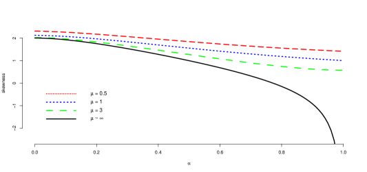
Figure 2: Skewness coefficient for $\mu=0.5,1,3$ and its limit as functions of $\alpha\in(0,1).$

Thus, the fPd is more flexible than the negative binomial, especially if the number of failures becomes large.

We applied the fractional Poisson model $\text{fPd}(\alpha,\mu)$ to two data sets, named Data $1$ and Data $2,$ which are about the reported incidents of crime that occurred in the city of Chicago from 2001 to present. The sample distributions together with their description are shown in Figure 3.

Figure 3: (Left) The number of all incidents from 2001-2018 for each police district. (Right) The number of incidents described as ”$\$500$ AND UNDER” for each police district.

Furthermore, we compared $\text{fPd}(\alpha,\mu)$ with the negative binomial $\text{NegBinom}(\text{size},\text{mean})$ using the usual chi-square goodness-of-fit test statistic and the maximum likelihood estimates for both models. Note that the chi-square test statistic follows, approximately, a chi-square distribution with $(k-1-p)$ degrees of freedom where $k$ is the number of cells and $p$ is the number of parameters to be estimated plus one.

For illustration purposes, we used grid search for the $\text{fPd}(\alpha,\mu)$ as it is relatively fast due to $\alpha$ being bounded in $(0,1)$ and to $\mu$, which is just in the neighborhood of the true data mean scaled by $\Gamma(1+\alpha).$ Observe that $5\times 10^{5}$ random numbers are used in all the calculations. From the results below, the fractional Poisson distribution $\text{fPd}(\alpha,\mu)$ provides better fits than the negative binomial $\text{NegBinom}(size,mean)$ model for both data sets at $5\%$ level of significance. This exercise clearly demonstrates the limitation of the negative binomial in dealing with left-skewed count data.

Table 1: Comparison between $\text{fPd}(\alpha,\mu)$ and $\text{NegBinom}(size,mean)$ fits.

Estimates	fPd	NegBinom
MLE for Data 1	$(\hat{\alpha},\hat{\mu})=(0.866,41574.1)$	$(size,mean)=(1.602,45590.17)$
MLE for Data 2	$(\hat{\alpha},\hat{\mu})=(0.85,3607)$	$(size,mean)=(1.69,4019.61)$
Chi-square for Data 1	71191.64	202542.7
Chi-square for Data 2	6442.634	21819.39
P-value for Data 1, $df=70939$	0.254	0
P-value for Data 2, $df=6442$	0.495	0

2.2 The case for gfPd$(\alpha,\alpha,1,\mu)$

When $\beta=\alpha$ and $\delta=1$, we have $X_{\alpha,\alpha}\;\stackrel{{\scriptstyle d}}{{=}}\;$gfPd$(\alpha,\alpha,1,\mu)$ with

$$P(X_{\alpha,\alpha}=x)=\Gamma(\alpha)\mu^{x}E_{\alpha,\alpha(x+1)}^{x+1}(-\mu),\qquad\mu>0;\,x\in\mathbb{N};\,\alpha\in(0,\;1].$$ (33)

Proposition 2.1.

The probability mass function can be written as

$$P(X_{\alpha,\alpha}=x)=\Gamma(\alpha+1)\frac{\mu^{x}}{x!}\int_{\mathbb{R}^{+}}y^{-\alpha(x+1)}e^{-\mu y^{-\alpha}}\nu_{S}(dy),$$ (34)

where $\nu_{S}$ is the distribution of a random variable $S$ whose density has Laplace transform $\exp(-t^{\alpha})$.

Proof.

Note that

$$\frac{1}{x!}\int_{\mathbb{R}^{+}}y^{-\alpha(x+1)}e^{-\mu y^{-\alpha}}\nu_{S}(dy)=\frac{1}{x!}\sum_{k\geq 0}\frac{(-\mu)^{k}}{k!}\int_{\mathbb{R}^{+}}y^{-\alpha k-\alpha(x+1)}\nu_{S}(dy)$$ (35)

$$=\frac{1}{x!}\sum_{k\geq 0}\frac{(-\mu)^{k}}{k!}\frac{\Gamma(1+k+x+1)}{\Gamma(1+\alpha k+\alpha(x+1))}=\sum_{k\geq 0}\frac{(-\mu)^{k}}{k!}\frac{\Gamma(k+x+1)}{\alpha x!\Gamma(\alpha k+\alpha(x+1))}$$

$$=\frac{1}{\alpha}E_{\alpha,\alpha(x+1)}^{x+1}(-\mu).$$

∎

The above result provides an algorithm to evaluate the probability mass function as

$$P(X_{\alpha,\alpha}=x) =\Gamma(\alpha+1)\frac{\mu^{x}}{x!}\bm{E}\left(S^{-\alpha(x+1)}e^{-\mu S^{-\alpha}}\right)$$ (36)

$$\approx\Gamma(\alpha+1)\frac{\mu^{x}}{x!}\left(\frac{1}{N}\sum_{j=1}^{N}S_{j}^{-\alpha(x+1)}e^{-\mu S_{j}^{-\alpha}}\right).$$

Thus, we can now estimate $\alpha$ and $\mu$ using maximum likelihood just like in the fPd case. The maximum likelihood estimates for the two crime datasets above are given in Table 2 below. The chi-square goodness-of-fit test statistics are large, indicating bad fits.

Table 2: Maximum likelihood estimates for $\text{gfPd}(\alpha,\alpha,1,\mu)$.

Estimates	$\text{gfPd}(\alpha,\alpha,1,\mu)$
MLE for Data 1	$(\hat{\alpha},\hat{\mu})=(0.844,38276)$
MLE for Data 2	$(\hat{\alpha},\hat{\mu})=(0.794,3020)$
Chi-square for Data 1	15609324
Chi-square for Data 2	966402.5

Remark 2.3.

From (2.1), the random variable $X_{\alpha,\alpha}$ has factorial moments

$$a_{k}=\frac{\Gamma(\alpha)\mu^{k}k!}{\Gamma(\alpha+\alpha k)},\qquad k\geq 0.$$ (37)

Thus the pgf is $G_{X_{\alpha,\alpha}}(u)=\Gamma(\alpha)E_{\alpha,\alpha}^{1}\left(\mu\left(u-1\right)\right)$, $|u|\leq 1$.

From (4) and (37), the symmetry structure of $X_{\alpha,\alpha}$ can be determined as follows:

$$\gamma(X_{\alpha,\alpha})=\frac{\Gamma(\alpha)\left(\frac{6}{\Gamma(4\alpha)}+\frac{6}{\mu\Gamma(3\alpha)}+\frac{1}{\mu^{2}\Gamma(2\alpha)}-\frac{6}{\Gamma(2\alpha)\Gamma(3\alpha)}+\frac{2}{\Gamma(2\alpha)^{3}}-\frac{3}{\mu\Gamma(2\alpha)^{2}}\right)}{\left(\frac{1}{\mu\Gamma(2\alpha)}+\frac{2}{\Gamma(3\alpha)}-\frac{1}{\Gamma(2\alpha)^{2}}\right)^{3/2}}.$$ (38)

Moreover,

$$\lim_{\mu\to\infty}\gamma(X_{\alpha,\alpha})=\frac{\Gamma(\alpha)\left(\frac{6}{\Gamma(4\alpha)}-\frac{6}{\Gamma(2\alpha)\Gamma(3\alpha)}+\frac{2}{\Gamma(2\alpha)^{3}}\right)}{\left(\frac{2}{\Gamma(3\alpha)}-\frac{1}{\Gamma(2\alpha)^{2}}\right)^{3/2}}\neq 0,$$ (39)

which vanishes if $\alpha=1$ (Poisson distribution). Moreover, (39) is non-negative and decreasing: this explains the bad fits indicated by the large chi-square values above.

3 Underdispersion and overdispersion for weighted Poisson distributions

Weighted Poisson distributions [30] provide a unifying approach for modelling both overdispersion and underdispersion [20]. Let $Y$ be a Poisson random variable of parameter $\lambda>0$ and let $Y^{w}$ be the corresponding WPD with weight function $w$.

Theorem 3.1.

If $\bm{E}w(Y+k)<\infty$ for all $k\in\mathbb{N}$, and $a_{k}=\lambda^{k}h(\lambda,k)$, where $h(\lambda,k)=\frac{\bm{E}w(Y+k)}{\bm{E}w(Y)}$, satisfies (5), then $Y^{w}$ has factorial moments $a_{k}$.

Proof.

It is enough to observe that the pgf $G_{Y^{w}}(u)$ can be written in form (2) as follows:

$$G_{Y^{w}}(u) =\sum_{k\geq 0}(u+1-1)^{k}\frac{e^{-\lambda}\lambda^{k}w(k)}{k!\bm{E}w(Y)}=\sum_{k\geq 0}\frac{(u-1)^{k}}{k!}\sum_{j\geq 0}\frac{e^{-\lambda}\lambda^{j+k}w(j+k)}{j!\bm{E}w(Y)}$$ (40)

$$=\sum_{k\geq 0}\frac{(u-1)^{k}}{k!}\lambda^{k}h(\lambda,k).$$

∎

Let $T$ be the linear left-shift operator acting on number sequences. Let us still denote with $T$ its coefficientwise extension to the ring of formal power series in ${\mathbb{R}}_{+}[[\lambda]]$ [34]. Next proposition links overdispersion and underdispersion of $Y^{w}$ respectively to a Turán-type and a reverse Turán-type inequality involving $T$.

Theorem 3.2.

The random variable $Y^{w}$ is overdispersed (underdispersed) if and only if

$$f(\lambda)T^{2}f(\lambda)>(<)\>[Tf(\lambda)]^{2},$$ (41)

where $f(\lambda)=\bm{E}w(Y)$.

Proof.

The random variable $Y^{w}$ is overdispersed if and only if $a_{2}>a_{1}^{2}$, that is $\bm{E}w(Y)\bm{E}w(Y+2)>[\bm{E}w(Y+1)]^{2}.$ Equivalently,

$$\left(\sum_{k\geq 0}\frac{\lambda^{k}}{k!}w(k)\right)\left(\sum_{k\geq 0}\frac{\lambda^{k}}{k!}w(k+2)\right)>\left(\sum_{k\geq 0}\frac{\lambda^{k}}{k!}w(k+1)\right)^{2},$$ (42)

and the result follows observing that $T^{j}f(\lambda)=\sum_{k\geq 0}\frac{\lambda^{k}}{k!}T^{j}[w(k)]$ for $j=1,2$. ∎

Remark 3.1.

Observe that when $w$ does not depend on $\lambda$, then $T^{j}f(\lambda)=D_{\lambda}^{j}f(\lambda)$ for $j=1,2.$ In this case, condition (41) is equivalent to $f(\lambda)D^{2}_{\lambda}f(\lambda)>(<)\>[D_{\lambda}f(\lambda)]^{2}$, i.e. log-convexity (log-concavity) of $f$. This is already known in the literature (see Theorem 3 of [20]).

Remark 3.2.

Note that from (42) we have

$$\sum_{k\geq 0}\frac{\lambda^{k}}{k!}\left(\sum_{j=0}^{k}\binom{k}{j}w(j)w(k-j+2)\right)>\sum_{k\geq 0}\frac{\lambda^{k}}{k!}\left(\sum_{j=0}^{k}\binom{k}{j}w(j+1)w(k-j+1)\right)$$ (43)

and some algebra leads us to the following sufficient condition for overdispersion or underdispersion: the random variable $Y^{w}$ is overdispersed (underdispersed) if

$$\sum_{j=0}^{k+1}\left[\binom{k}{j}-\binom{k}{j-1}\right]w(j)w(k-j+2)>(<)\>0.$$ (44)

Notice that $\bm{E}w(Y)$ is a function of the Poisson parameter $\lambda$. For the sake of clarity, from now on, let us denote it by $\eta(\lambda)$. Weighted Poisson distributions with a weight function $w$ not depending on the Poisson parameter $\lambda$ are also known as power series distributions (PSD) [14] and it is easy to see that the factorial generating function in this case reads

$$Q(t)=\frac{\eta[\lambda(t+1)]}{\eta(\lambda)}$$ (45)

with factorial moments

$$a_{r}=\frac{\lambda^{r}}{\eta(\lambda)}\frac{d^{r}}{d\lambda^{r}}[\eta(\lambda)],\qquad r\geq 1.$$ (46)

A special well-known family of PSD is the generalized hypergeometric probability distribution (GHPD) [17], where

$$Q(t)=\frac{{}_{p}F_{q}\left[(a);(b);\lambda(t+1)\right]}{{}_{p}F_{q}\left[(a);(b);t\right]}$$ (47)

with ${}_{p}F_{q}$ given in (9). Depending on the values of the parameters of GHPD both overdispersion and underdispersion are possible [37]. For $p=q=1,$ a special case of GHPD is the hyper-Poisson distribution [2]. In the next section we will analyze an alternative WPD in which the hyper-Poisson distribution remains a special case and that exhibits both underdispersion and overdispersion.

3.1 A novel flexible WPD allowing overdispersion or underdispersion

Let $Y^{w}$ be a WP random variable with weight function

$$w(k)=\frac{\Gamma(k+\gamma)}{\Gamma(\alpha k+\beta)^{\nu}},$$ (48)

where $\gamma>0$, $\min(\alpha,\beta,\nu)\geq 0$, $\alpha+\beta>0$. Moreover, if $\gamma=\beta$ and $\nu\geq 1$ then $\beta$ is allowed to be zero. Since it is a PSD, the random variable $Y^{w}$ is characterized by the normalizing function

$$\eta(\lambda)=\eta_{\alpha,\beta}^{\gamma,\nu}(\lambda)=\sum_{k=0}^{\infty}\frac{\lambda^{k}}{k!}\frac{\Gamma(k+\gamma)}{\Gamma(\alpha k+\beta)^{\nu}}.$$ (49)

The convergence of the above series can be ascertained as follows. Let $\gamma\leq 1$; by Gautschi’s inequality (see [36], formula (2.23)) we have the upper bound

$$\eta(\lambda)\leq\frac{\Gamma(\gamma)}{\Gamma(\beta)^{\nu}}+\sum_{k=1}^{\infty}\frac{\lambda^{k}k^{\gamma-1}}{\Gamma(\alpha k+\beta)^{\nu}},$$ (50)

which converges by ratio test and taking into account the well-known asymptotics for the ratio of gamma functions (see [38]). Now, let $\gamma>1$. In this case an upper bound can be derived by formula (3.72) of [36]:

$$\eta(\lambda)<\frac{\Gamma(\gamma)}{\Gamma(\beta)^{\nu}}+\sum_{k=1}^{\infty}\frac{\lambda^{k}(k+\gamma)^{\gamma-1}}{\Gamma(\alpha k+\beta)^{\nu}}.$$ (51)

Again, this converges by ratio test and recurring to the above-mentioned asymptotic behaviour of the ratio of gamma functions.

The random variable $Y^{w}$ specializes to some well-known classical random variables. Specifically, we recognize the following:

1. If $\gamma=\beta=\alpha=\nu=1$, we recover the Poisson distribution as the weights equal unity for each $k$.

2. If $\gamma=\beta=\alpha=1$, we recover the COM-Poisson distribution [8] of Poisson parameter $\lambda$ and dispersion parameter $\nu$.

3. If $\gamma=\alpha=\nu=1$ we obtain the hyper-Poisson distribution [2].

4. If $\gamma=\nu=1$ we obtain the alternative Mittag–Leffler distribution considered e.g. in [2] and [13].

5. If $\gamma=1$ we recover the fractional COM-Poisson distribution [12].

6. If $\nu=1$ we obtain the alternative generalized Mittag-Leffler distribution [35].

Since $Y^{w}$ is a PSD, it is easy to derive its factorial moments,

$$a_{r}=\frac{\lambda^{r}}{\eta_{\alpha,\beta}^{\gamma,\nu}(\lambda)}\sum_{k=r}^{\infty}\frac{\lambda^{k-r}}{(k-r)!}\frac{\Gamma(k+\gamma)}{\Gamma(\alpha k+\beta)^{\nu}}=\lambda^{r}\frac{\eta_{\alpha,\alpha r+\beta}^{\gamma+r,\nu}(\lambda)}{\eta_{\alpha,\beta}^{\gamma,\nu}(\lambda)},$$ (52)

from which the moments are immediately derived by recalling formula (3).

Remark 3.3.

Since $\eta_{\alpha,\alpha r+\beta}^{\gamma+r,\nu}(\lambda)=\sum_{j\geq 0}\frac{\lambda^{j}}{j!}A_{j,r}$ with

$$A_{j,r}=\frac{\Gamma(j+r+\gamma)}{\Gamma[\alpha(j+r)+\beta)]^{\nu}},$$ (53)

by using Faà di Bruno’s formula [34] one has

$$a_{r}=\lambda^{r}\sum_{j\geq 0}\frac{\lambda^{j}}{j!}\sum_{i=0}^{j}\binom{j}{i}A_{j-i,r}D_{i}\quad\text{with}\quad D_{i}=\sum_{k=0}^{i}(-1)^{k}A_{0,0}^{-(k+1)}{\mathfrak{B}}_{i,k}(A_{1,0},\ldots,A_{i-k+1,0}),$$ (54)

where $\{A_{j,0}\}$ and and $\{{\mathfrak{B}}_{i,k}\}$ are the coefficients of $\eta_{\alpha,\beta}^{\gamma,\nu}(\lambda)$ and the partial Bell exponential polynomials [34], respectively.

Furthermore, the probability mass function reads

$$P(Y^{w}=x)=\frac{\lambda^{x}}{x!}\frac{\Gamma(x+\gamma)}{\Gamma(\alpha x+\beta)^{\nu}}\frac{1}{\eta_{\alpha,\beta}^{\gamma,\nu}(\lambda)},\qquad x\geq 0.$$ (55)

Concerning the variability of $Y^{w}$, by using Theorem 3 of [20], the preceding Lemma and the succeeding Corollary, that is by imposing log-convexity (log-concavity) of the weight function, we write for $y\in\mathbb{R}_{+}$,

$$\frac{d^{2}}{dy^{2}}\log\frac{\Gamma(y+\gamma)}{\Gamma(\alpha y+\beta)^{\nu}} =\frac{d}{dy}\left[\frac{1}{\Gamma(y+\gamma)}\frac{d}{dy}\Gamma(y+\gamma)-\frac{\nu}{\Gamma(\alpha y+\beta)}\frac{d}{dy}\Gamma(\alpha y+\beta)\right]$$ (56)

$$=\frac{d}{dy}\left[\psi(y+\gamma)-\nu\alpha\,\psi(\alpha y+\beta)\right],$$

where $\psi(z)$ is the Psi function (see [22], Section 1.3). In addition, by considering formula (6.4.10) of [1],

$$\frac{d^{2}}{dy^{2}}\log\frac{\Gamma(y+\gamma)}{\Gamma(\alpha y+\beta)^{\nu}}=\sum_{r=0}^{\infty}(y+\gamma+r)^{-2}-\nu\alpha^{2}\sum_{r=0}^{\infty}(\alpha y+\beta+r)^{-2}.$$ (57)

Therefore log-convexity (log-concavity) of $w(y)$ is equivalent to the condition

$$\nu<(>)\,\frac{\sum_{r=0}^{\infty}(y+\gamma+r)^{-2}}{\alpha^{2}\sum_{r=0}^{\infty}(\alpha y+\beta+r)^{-2}},\qquad\forall\>y\in\mathbb{R}_{+}.$$ (58)

This yields that if (58) holds, then $Y^{w}$ is overdispersed (underdispersed).

Remark 3.4 (Classical special cases).

If $\alpha=\beta=\gamma=1$, then $Y^{w}$ is the COM-Poisson random variable and (58) correctly reduces to the ranges $\nu>1$ giving underdispersion and $\nu\in[0,1)$ giving overdispersion. If $\alpha=\gamma=\nu=1$, then $Y^{w}$ is the hyper-Poisson random variable and (58) correctly reduces to the ranges $\beta>1$ (overdispersion) and $\beta\in[0,1)$ (underdispersion). This holds as $\beta\mapsto\sum_{r=0}^{\infty}(y+\beta+r)^{-2}$ is decreasing for all fixed $y\in\mathbb{R}_{+}$.

In the two next sections we analyze two special cases of interest, the first of which, to the best of our knowledge, is still not considered in the literature.

3.1.1 Model I

We first introduce the special case in which $\alpha=1$, $\gamma=\beta$, $\beta>0$, and $\beta$ is allowed to be zero only if $\nu\geq 1$. This is a three-parameter ($\lambda,\nu,\beta$) model which retains the same simple conditions for underdispersion and overdispersion as for the COM-Poisson model. Indeed, formula (58) reduces to $\nu>1$ and $\nu\in[0,1)$, respectively. However, this model is more flexible than the COM-Poisson model because of the presence of the parameter $\beta$. Notice that the pmf can be written as

$$P(Y^{w}=x)=\frac{1}{x!}\exp\left(x\log\lambda+(1-\nu)\log\Gamma(x+\beta)-\log\eta_{1,\beta}^{\beta,\nu}(\lambda)\right),$$ (59)

which suggests that Model I belongs to the exponential family of distributions with parameters $\log\lambda$ and $1-\nu$, where $\beta$ is a nuisance parameter or is known. Figures 4 and 5 show sample shapes of this family of distributions.

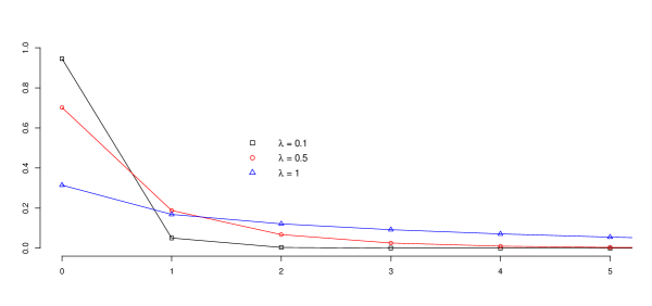
Figure 4: Probability mass functions (59) for $\lambda=0.1,0.5,1$, $\beta=0.5$, and $\nu=0.1.$

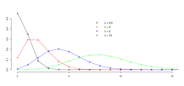
Figure 5: Probability mass functions (59) for $\lambda=0.5,2,5,10$, $\beta=0.1$, and $\nu=1.1.$

Note that distributions in Figure 4 (Figure 5) are overdispersed (underdispersed). Also,

$$P(Y^{w}=x+1)=\frac{\lambda}{(x+1)(x+\beta)^{\nu-1}}P(Y^{w}=x).$$ (60)

This gives a procedure to calculate iteratively the probability mass function and generate random numbers. The only thing to figure out is to compute $\eta_{1,\beta}^{\beta,\nu}(\lambda)$ in order to obtain $P(Y^{w}=0)=1/[\Gamma(\beta)^{\nu-1}\eta_{1,\beta}^{\beta,\nu}(\lambda)]$.

An upper bound for the normalizing function $\eta_{1,\beta}^{\beta,\nu}(\lambda)$ can be determined similarly to [26], Section 3.2, taking into consideration that the multiplier

$$\lambda(j+\beta)^{1-\nu}/(j+1)$$ (61)

is ultimately monotonically decreasing. Hence, we can approximate the normalizing constant $\eta_{1,\beta}^{\beta,\nu}(\lambda)$ by truncating the series and bound the truncation error $R_{\widetilde{k}}$,

$$\eta_{1,\beta}^{\beta,\nu}(\lambda) =\sum_{j=0}^{\widetilde{k}}\frac{\lambda^{j}}{j!}\Gamma(j+\beta)^{1-\nu}+R_{\widetilde{k}}$$ (62)

$$<\sum_{j=0}^{\widetilde{k}}\frac{\lambda^{j}}{j!}\Gamma(j+\beta)^{1-\nu}+\frac{\lambda^{\widetilde{k}+1}\Gamma(\widetilde{k}+1+\beta)^{1-\nu}}{(\widetilde{k}+1)!}\sum_{j=0}^{\infty}\varepsilon_{\widetilde{k}}^{j}$$

$$<\sum_{j=0}^{\widetilde{k}}\frac{\lambda^{j}}{j!}\Gamma(j+\beta)^{1-\nu}+\frac{\lambda^{\widetilde{k}+1}\Gamma(\widetilde{k}+1+\beta)^{1-\nu}}{(\widetilde{k}+1)!\,(1-\varepsilon_{\widetilde{k}})},$$

where $\widetilde{k}$ is such that for $j>\widetilde{k}$ the multiplier (61) is already monotonically decreasing and bounded above by $\varepsilon_{\widetilde{k}}\in(0,1)$. Correspondingly, denoting with $\widetilde{\eta}_{1,\beta}^{\beta,\nu}(\lambda)=\sum_{j=0}^{\widetilde{k}}\frac{\lambda^{j}}{j!}\Gamma(j+\beta)^{1-\nu}$, the relative truncation error $R_{\widetilde{k}}/\widetilde{\eta}_{1,\beta}^{\beta,\nu}(\lambda)$ is bounded by

$$\frac{\lambda^{\widetilde{k}+1}\Gamma(\widetilde{k}+1+\beta)^{1-\nu}}{(\widetilde{k}+1)!\,(1-\varepsilon_{\widetilde{k}})\widetilde{\eta}_{1,\beta}^{\beta,\nu}(\lambda)}.$$ (63)

As a last remark, we can further simplify the model obtaining a two-parameter model. In order to do so, let $\nu=\beta$, with $\beta>0$. The obtained model still allows for underdispersion ($\beta>1$) and overdispersion ($\beta\in(0,1)$) and it should be directly compared with the COM-Poisson and the hyper-Poisson models.

3.1.2 Model II

If we set $\alpha=\nu=1$ we get another three-parameter ($\lambda,\gamma,\beta$) model, special case of the alternative generalized Mittag-Leffler distribution (see point 6 above). The reparametrization $\beta=\xi\gamma$ together with condition (58) shows that both overdispersion ($\xi>1$) and underdispersion ($\xi\in(0,1)$) are possible. This comes from the fact that $\omega\mapsto\sum_{r=0}^{\infty}(y+\omega+r)^{-2}$ is decreasing for all fixed $y\in\mathbb{R}_{+}$. As for Model I, the probability distribution belongs to the exponential family with parameter $\log\lambda,$ with $\gamma$ and $\beta$ as nuisance parameters. Explicitly, the pmf reads

$$P(Y^{w}=x)=\frac{\lambda^{x}}{x!}\frac{\Gamma(x+\gamma)}{\Gamma(x+\beta)}\frac{1}{\eta_{1,\beta}^{\gamma,1}(\lambda)},\qquad x\geq 0,$$ (64)

and, as in the previous Section 3.1.1, the iterative representation

$$P(Y^{w}=x+1)=\frac{\lambda(x+\gamma)}{(x+1)(x+\beta)}P(Y^{w}=x),$$ (65)

allows an approximated evaluation of the pmf with error control, and consequently random number generation. Also in this case this holds as the involved multiplier is ultimately monotonically decreasing. Figures 6 and 7 show some forms of this class of distributions. Observe that distributions in Figure 6 (Figure 7) are underdispersed (overdispersed).

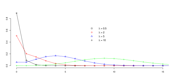
Figure 6: Probability mass functions (64) for $\lambda=0.5,2,5,10$, $\beta=0.5$, and $\gamma=0.1.$

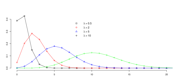
Figure 7: Probability mass functions (64) for $\lambda=0.5,2,5,10$, $\beta=0.1$, and $\gamma=1.1.$

If we further let $\lambda=1$, we obtain a two-parameter model, still allowing for underdispersion if $\beta\in(0,\gamma)$ (or equivalently $\xi\in(0,1)$) and overdispersion if $\beta>\gamma$ (or $\xi>1$), which is also directly comparable with the two-parameter Model I above, the COM-Poisson model, and the hyper-Poisson model.

3.1.3 Comparison

We now compare Model I and Model II with known models that allow overdispersion and underdispersion such as the COM-Poisson, generalized Poisson and hyper-Poisson models as cited above. Note that the hyper-Poisson distribution satisfies

$$P(Y^{w}=x+1)=\frac{\lambda}{(x+\beta)}P(Y^{w}=x).$$ (66)

For comparison purposes, we first consider the number of fish caught data shown in Figure 8 (left panel) below. The dataset corresponds to 239 groups (as 11 potential outliers were removed) that went to a state park and state wildlife biologists asked visitors how many fish they caught. The mean fish caught is around 1.48 while the variance is 8.04. Furthermore, the optimx (for hyper-Poisson, Model I and Model II), COMPoissonReg (for COM-Poisson), compoisson (for COM-Poisson), and VGAM (for generalized Poisson) packages in R are used for the maximum likelihood estimation and the chi-square goodness-of-fit tests. In particular, the L-BFGS-B method from the optimx package is used and 1000 terms were summed for the normalizing constant $\eta_{\alpha,\beta}^{\gamma,\nu}(\lambda)$. Just like the comparisons above, a chi-square distribution is used as reference where the degrees of freedom is the number of cells minus the number of model parameters. From Table 3, Model I and Model II clearly outperform the other models although the generalized Poisson and hyper-Poisson (subcase of WPD) also provide good fits to the fish count data.

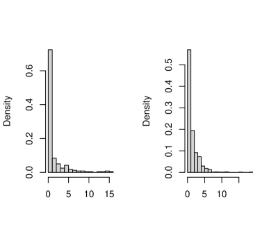
Figure 8: (Left) The fish caught count data. (Right) The count of articles produced by graduate students in biochemistry Ph.D. programs.

Table 3: Comparison results for the fish count data.

Model	ML Estimates	Chi-square	P-value
COM-Poisson	$(\hat{\lambda},\hat{\nu})=(11.5876,0.9806)$	$13495000$	0
Hyper-Poisson	$(\hat{\alpha},\hat{\beta})=(37.1126,170)$	$18.2259$	0.1090
Gen Poisson	$(\hat{\lambda},\hat{\theta})=(0.6334,0.5430)$	$15.1197$	0.2349
Model I	$(\hat{\alpha},\hat{\beta},\hat{\nu})=(0.9544,0.2126,0.0632)$	$12.6350$	0.3178
Model II	$(\hat{\alpha},\hat{\beta},\hat{\gamma})=(134.5545,149.9958,0.2504)$	$\bm{9.7697}$	$\bm{0.5512}$

We have also considered the bioChemists data from the pscl package in R, particularly the count of articles produced by 915 graduate students in biochemistry Ph.D. programs during last 3 years in the program. The data has mean 1.69 and variance of 3.71, and is showcased in Figure 8 (right panel). Apparently, Table 4 suggests that Model II outperforms the rest of the models considered for the article count data. Overall, there is potential in WPD’s (e.g., Model I and Model II) in flexibly capturing overdispersed and/or underdispersed count data distributions.

Table 4: Comparison results for the article count data.

Model	ML Estimates	Chi-square	P-value
COM-Poisson	$(\hat{\lambda},\hat{\nu})=(14.4428,0.9903)$	$14156763$	0
Hyper-Poisson	$(\hat{\alpha},\hat{\beta})=(14.5253,20.3124)$	$1549.086$	1.3487e-34
Gen Poisson	$(\hat{\lambda},\hat{\theta})=(0.2991,1.1886)$	$121.9043$	8.0757e-19
Model I	$(\hat{\alpha},\hat{\beta},\hat{\nu})=(0.4992,1.7028,0.001)$	$266.8644$	9.229e-49
Model II	$(\hat{\alpha},\hat{\beta},\hat{\gamma})=(73.17587,150.001,1.7985)$	$\bm{21.4124}$	$\bm{0.0915}$

Acknowledgments

F. Polito has been partially supported by the project “Memory in Evolving Graphs” (Compagnia di San Paolo/Università degli Studi di Torino).

References

• Abramowitz and Stegun [1964] Abramowitz M. and Stegun I.A. (1964) Handbook of mathematical functions with formulas, graphs, and mathematical tables. National Bureau of Standards Applied Mathematics Series. 55, pp. 1046.
• Crow and Bardwell [1964] Bardwell G. E. and Crow E. L. (1964) A two-parameter family of hyper-Poisson distributions. Journal of the American Statistical Association, 59, 133–141.
• Beghin and Orsingher [2009] Beghin L. and Orsingher E. (2009) Fractional Poisson processes and related planar random motions. Electronic Journal of Probability, 14, 1790–1826.
• Beghin and Orsingher [2010] Beghin L. and Orsingher E. (2010) Poisson-type processes governed by fractional and higher-order recursive differential equations. Electronic Journal of Probability, 15(22), 684–709.
• Cahoy et al. [2010] Cahoy D.O., Uchaikin V.V. and Woyczynski W.A. (2010) Parameter estimation for fractional Poisson processes. Journal of Statistical Planning and Inference, 140(11), 3106–3120.
• Chambers et. al [1976] Chambers J. M., Mallows C. L. and Stuck, B. W. (1976) A method for simulating stable random variables. Journal of the American Statistical Association, 71(354), 340–344.
• Consul and Jain [1973] Consul P. C. and Jain G. C. (1973) A generalization of the Poisson distribution. Technometrics, 15, 791–799.
• Conway et al. [1962] Conway R. W. and Maxwell W. L. (1962) A queuing model with state dependent service rates. Journal of Industrial Engineering, 12, 132–136.
• Daley and Narayan [1980] Daley D. J. and Narayan P. (1980) Series expansions of probability generating functions and bounds for the extinction probability of branching process. Journal of Applied Probability, 17(4), 939–947.
• De Oliveira et al. [2011] De Oliveira E. C., Mainardi F. and Vaz J. (2011) Models based on Mittag-Leffler functions for anomalous relaxation in dielectrics. The European Physical Journal Special Topics, 193(1), 161–171.
• Di Nardo et al. [2006] Di Nardo E. and Senato D. (2006) An umbral setting for cumulants and factorial moments. European Journal of Combinatorics, 27, 394–413.
• Garra et al. [1948] Garra R., Orsingher E. and Polito F. (2018) A Note on Hadamard Fractional Differential Equations with Varying Coefficients and Their Applications in Probability. Mathematics, 6(1), 4, 10pp.
• Herrmann [2016] Herrmann R. (2016) Generalization of the fractional Poisson distribution. Fractional Calculus and Applied Analysis, 19(4), 832–842.
• Johnson et al. [2005] Johnson N. L., Kemp A. W. and Kotz S. (2005) Univariate discrete distributions. III edition. Wiley Series in Probability and Statistics. John Wiley $\&$ Sons.
• Jumarie [2001] Jumarie G. (2012) Fractional master equation: non-standard analysis and Liouville-Riemann derivative. Chaos, Solutions and Fractals, 12, 2577–2587.
• Kanter [1975] Kanter M. (1975) Stable densities under change of scale and total variation inequalities. The Annals of Probability, 3(4), 697–707.
• Kemp [1968] Kemp A. W. (1968) A wide class of discrete distributions and the associated differential equations. Sankhya (A), 30, 401-410.
• Kemp and Kemp [1974] Kemp A. and Kemp C. (1974) A family of discrete distributions defined via their factorial moments. Communications in Statistics, 3(12), 1187–1196.
• Kilbas et al. [2006] Kilbas A. A., Srivastava H. M. and Trujillo J. J. (2006) Theory and applications of fractional differential equations. North-Holland Mathematics Studies, 204. Elsevier Science B.V., Amsterdam.
• Kokonendji et al. [2006] Kokonendji C. C., Mizère D. and Balakrishnan N. (2008) Connections of the Poisson weight function to overdispersion and underdispersion. Journal of Statistical Planning Inference, 138(5), 1287–1296.
• Laskin [2003] Laskin N. (2003) Fractional Poisson process. Communications in Nonlinear Science and Numerical Simulation, 8, 201–213.
• Lebedev [1972] Lebedev N. N. (1972) Special functions and their applications, Dover Publications, Inc., New York.
• Maceda [1948] Maceda E.C . (1948) On the compound and generalized Poisson distributions. Annals of Mathematical Statistics, 19, 414–416.
• Mainardi et al. [2010] Mainardi F., Mura A. and Pagnini G. (2010) The $M$-Wright function in time-fractional diffusion processes: a tutorial survey. International Journal of Differential Equations, Art. ID 104505, 29 pp.
• Meerschaert et al. [2011] Meerschaert M.M., Nane E. and Vellaisamy P. (2011) The fractional Poisson process and the inverse stable subordinator. Electronic Journal of Probability, 16, 1600–1620.
• Minka et al. [2003] Minka T.P., Shmueli G., Kadane J.B., Borle S. and Boatwright P. (2003) Computing with the COM-Poisson distribution. Technical Report 775. Department of Statistics, Carnegie Mellon University, Pittsburgh. (Available from http://www.stat.cmu.edu/tr/)
• Polito and Tomovski [2016] Polito F. and Tomovski Ž. (2016) Some properties of Prabhakar-type fractional calculus operators. Fractional Differential Calculus, 6(1), 73–94.
• Potts [1953] Potts R. B. (1953) Note on the factorial moments of standard distributions. Australian Journal of Physics, 6(4), 498–499.
• Prabhakar [1971] Prabhakar T.R. (1971). A singular integral equation with a generalized Mittag-Leffler function in the kernel. Yokohama Mathematical Journal, 19, 7–15.
• Rao [1965] Rao C. R. (1965) On discrete distributions arising out of methods of ascertainment. Sankhyā (A), 27, 311–324.
• Saichev and Zaslavsky [1997] Saichev A.I. and Zaslavsky G.M. (1997) Fractional kinetic equations: solutions and applications. Chaos, 7(4), 753–764.
• Shmueli et al. [2005] Shmueli G., Minka T.P., Kadane J., Borle S. and Boatwright, P. (2005) A useful distribution for fitting discrete data: revival of the Conway-Maxwell-Poisson distribution, Journal of the Royal Statistical Society, Series C (Applied Statistics), 54(1), 127–142.
• Repin and Saichev [2000] Repin O.N. and Saichev A.I. (2000) Fractional Poisson law. Radiophysics and Quantum Electronics, 43(9), 738–741.
• Stanley [2012] Stanley R.P. (2012) Enumerative combinatorics. Vol.1, Cambridge Studies in Advanced Mathematics, 49, Cambridge University Press.
• Pogany and Tomovski [2016] Pogány T.K. and Tomovski Z. (2016) Probability distribution built by Prabhakar function. Related Turán and Laguerre inequalities. Integral Transforms and Special Functions, 27(10), 783–793.
• Qi [2010] Qi F. (2010) Bounds for the ratio of two gamma functions. Journal of Inequalities and Applications, Art. ID 493058, 84 pp.
• Tripathi and Gurland [1979] Tripathi R. C. and Gurland J. (1979) Some aspects of the Kemp families of distributions. Comm. Statist. A - Theory Methods, 8, 855–869.
• Tricomi and Erdélyi [1951] Tricomi F. G. and Erdélyi A. (1951) The asymptotic expansion of a ratio of gamma functions. Pacific Journal of Mathematics, 1, 133–142.