Families of Multidimensional Arrays with Good Autocorrelation and Asymptotically Optimal Cross-correlation

Abstract

We introduce a construction for families of $2n$-dimensional arrays with asymptotically optimal pairwise cross-correlation. These arrays are constructed using a circulant array of $n$-dimensional Legendre arrays. We also introduce an application of these higher-dimensional arrays to high-capacity digital watermarking of images and video.

1 Background

Biphase sequence families with low periodic off peak autocorrelation and low cross-correlation are highly sought after for CDMA wireless communications. This has been an active research area since the landmark paper of Gold in 1967[7], and numerous constructions of such families are known.

The concept of binary two-dimensional doubly periodic arrays with optimal off-peak autocorrelation was introduced by Gordon in 1966[8]. Such arrays are two-dimensional analogues of m-sequences. They are either solitary, or have very small family sizes called maximal connected sets[17], and higher-dimensional families are rare[9]. Perfect binary arrays in two and higher-dimensions have also been studied[11], but they are solitary, and most have unfavourable aspect ratios for applications. In 1988, Lüke surveyed existing constructions of two-dimensional arrays[14]. In 1989, the Legendre sequences were generalised to two and higher-dimensional analogues[15][6].

Two and three-dimensional arrays find applications in optics, where they are used for coded aperture imaging, or in structured light, where they are used for image alignment or registration. The first families of two-dimensional arrays were constructed in 1991 by Green et al[10], where the small Kasami and No–Kumar sequences were interpreted as arrays.

In 1997, Tirkel et al, motivated by finding two-dimensional patterns for use as spread spectrum watermarks, constructed families of arrays. The arrays were of size $p\times p$, where $p$ is a prime number. Later this was extended to $p\times p-1$, $p\times p+1$, and $p-1\times p+1$ [13] and to higher dimensions[2].

The periodic cross-correlation of two $N$-dimensional arrays, A and B, both of size $l_{0}\times l_{1}\times\cdots\times l_{N-1}$, for shift $s_{0},s_{1},\cdots,s_{N-1}$ is defined as

$$\theta_{\textbf{A},\textbf{B}}\left(s_{0},s_{1},\cdots,s_{N-1}\right)=\sum_{i_{0}=0}^{l_{0}-1}\sum_{i_{1}=0}^{l_{1}-1}\cdots\sum_{i_{N-1}=0}^{l_{N-1}-1}A_{i_{0},i_{1},\cdots,i_{N-1}}B_{i_{0}+s_{0},i_{1}+s_{1},\cdots,i_{N-1}+s_{N-1}}^{*}.$$

Similarly, the periodic autocorrelation of a $N$-dimensional array for shift $s_{0},s_{1},\cdots,s_{N-1}$ is given by $\theta_{\textbf{A}}\left(s_{0},s_{1},\cdots,s_{N-1}\right)=\theta_{\textbf{A},\textbf{A}}\left(s_{0},s_{1},\cdots,s_{N-1}\right)$. $\theta_{\textbf{A}}(s_{0},s_{1},\cdots,s_{N-1})$ is called an off-peak autocorrelation if not all $s_{i}=0\text{ mod }l_{i}$. We denote the array of all autocorrelations and cross-correlations for all shifts as $\theta_{\textbf{A}}$ and $\theta_{\textbf{A},\textbf{B}}$ respectively.

Sequences with flat periodic autocorrelation which used properties of the Legendre symbol were first discovered by Lerner in 1958[12], where the sequences were termed Legendre sequences. In the same year, Zierler showed the Legendre sequences possessed flat periodic autocorrelation[21].

Definition 1.1.

(Legendre Sequences)[21] Let s be a sequence of length $p$, for $p$ an odd prime. Then

$$s_{k}=\begin{cases}a&\text{if $k=0$}\\ 1&\text{if $k$ is a quadratic residue mod $p$}\\ -1&\text{otherwise}\end{cases}$$

for $0\leq k<p$.

If $a=0$, then all off-peak autocorrelations of the Legendre sequences equal to -1. If $a=\pm 1$, then all off-peak autocorrelations of the Legendre sequences $-1$ when $p=4k-1$, and $1$ and $-3$ otherwise.

Example 1.2.

We construct the length 17 Legendre sequence and compute its periodic autocorrelations.

$$\textbf{s}=[0,1,1,-1,1,-1,-1,-1,1,1,-1,-1,-1,1,-1,1,1],$$

$$\theta_{\textbf{s}}=[16,-1,-1,-1,-1,-1,-1,-1,-1,-1,-1,-1,-1,-1,-1,-1,-1].$$

In 1990, Bömer and Antweiler introduced a construction of two-dimensional Legendre arrays of sizes $p\times p$ where $p$ is an odd prime[5]. These arrays possessed flat autocorrelation, with all off-peak autocorrelations equal to -1.

Definition 1.3.

(Legendre arrays)[5] Let $\alpha$ be a primitive element in $\text{GF}\left(p^{2}\right)$, then every power of $\alpha$ can be expressed as

$$\alpha^{i}=m\,\alpha+n$$

where $0\leq i<p^{2}-1$ and $(m,n)\neq(0,0)$. Then the two-dimensional Legendre array, A, is given by

$$A_{m,n}=\begin{cases}$a$&\text{if $(m,n)=(0,0)$}\\ $+1$&\text{if $\alpha^{2r}=m\,\alpha+n$}\\ $-1$&\text{if $\alpha^{2r+1}=m\,\alpha+n$}\end{cases}$$

If $a=0$, then all the off-peak periodic autocorrelations are $-1$, and if $a=\pm 1$ then all the off-peak periodic autocorrelations are $\pm 1$ and $\pm 3$.

Example 1.4.

Let $p=5$, then $x^{2}+4x+2$ is a primitive polynomial in $\text{GF}\left(p^{2}\right)$, and the $5\times 5$ Legendre array, A, is given by

$$\left[\begin{array}[]{ccccc}0&1&1&1&1\\ -1&-1&-1&1&1\\ -1&1&-1&1&-1\\ -1&-1&1&-1&1\\ -1&1&1&-1&-1\\ \end{array}\right]$$

where $a=0$.

This construction readily generalises to $n$-dimensions by using a primitive polynomial of degree $n$ in $\text{GF}\left(p^{n}\right)$.

Example 1.5.

Consider the construction of a 4D Legendre array. Let $p=3$, then $x^{4}+2x^{3}+2$ is a primitive polynomial in $\text{GF}\left(p^{4}\right)$, and the $3\times 3\times 3\times 3$ Legendre array, A, is given by

$$\textbf{A}=\left[\begin{array}[]{ccc}\left[\begin{array}[]{ccc}0&1&1\\ -1&-1&1\\ -1&1&-1\\ \end{array}\right]&\left[\begin{array}[]{ccc}1&1&-1\\ 1&1&-1\\ -1&1&1\\ \end{array}\right]&\left[\begin{array}[]{ccc}1&-1&1\\ -1&1&1\\ 1&-1&1\\ \end{array}\right]\\ \left[\begin{array}[]{ccc}-1&-1&1\\ -1&-1&-1\\ 1&1&-1\\ \end{array}\right]&\left[\begin{array}[]{ccc}-1&1&1\\ -1&-1&1\\ 1&1&1\\ \end{array}\right]&\left[\begin{array}[]{ccc}1&-1&1\\ -1&-1&1\\ -1&-1&-1\\ \end{array}\right]\\ \left[\begin{array}[]{ccc}-1&1&-1\\ 1&-1&1\\ -1&-1&-1\\ \end{array}\right]&\left[\begin{array}[]{ccc}1&1&-1\\ -1&-1&-1\\ -1&1&-1\\ \end{array}\right]&\left[\begin{array}[]{ccc}-1&1&1\\ 1&1&1\\ -1&1&-1\\ \end{array}\right]\\ \end{array}\right]$$

In 2017, Blake and Tirkel introduced a construction for multi-dimensional, block-circulant perfect autocorrelation arrays[1][4]. A special case of this construction is a two-dimensional perfect array, constructed from a circulant array[3, const. XII, pp. 38].

Definition 1.6.

[3] Let ${\bf a}=\left[a_{0},a_{1},\cdots,a_{n-1}\right]$ and $\textbf{c}=\left[c_{0},c_{1},\cdots,c_{n-1}\right]$ be perfect sequences – each of length $n$. We construct an array, S, such that

$$\textbf{S}=\left[S_{i,j}\right]=a_{j}\,c_{i+j\text{ mod }n},$$

where $0\leq i,j<n$.

The sequence, a, is termed the multiplication sequence.

2 The multidimensional construction

We now introduce a construction for families of $2n$-dimensional arrays.

Definition 2.1.

Let $A$ be a $n$-dimensional Legendre array of size $p\times p\times\cdots\times p$, where $p$ is an odd prime. Then we construct a family of $p$, $2n$-dimensional arrays, $\textbf{S}_{m}$, for $0\leq m<p$, where

$$\textbf{S}_{m}=\left[S_{i_{0},i_{1},\cdots,i_{2n-1}}\right]_{m}=A_{i_{0},i_{1},\cdots,i_{n-1}}\,A_{m\,i_{0}+i_{n}\text{ mod }p,m\,i_{1}+i_{n+1}\text{ mod }p,\cdots,m\,i_{n-1}+i_{2n-1}\text{ mod }p},$$

where $0\leq i_{0},i_{1},\cdots,i_{2n-1}<p$.

Similarities between this construction and the 2D circulant construction are clearly evident. In particular, the multiplication sequence $a_{j}$ and its counterpart the multiplication array $A_{i_{0},i_{1},\cdots,i_{n-1}}$; and the circulant array of columns $\,c_{i+j\text{ mod }n}$ and its counterpart $A_{m\,i_{0}+i_{n}\text{ mod }p,m\,i_{1}+i_{n+1}\text{ mod }p,\cdots,m\,i_{n-1}+i_{2n-1}\text{ mod }p}$.

Theorem 2.2.

When $a$ (the first entry in the multidimensional Legendre array) is zero, the magnitude of the off-peak periodic autocorrelation of $\textbf{S}_{m}$ is bounded by $p^{n}-1$.

Proof.

The periodic autocorrelation of $\textbf{S}_{m}$ for an off-peak shift $s_{0},s_{1},\cdots,s_{2n-1}$ is given by

$$\theta_{\textbf{S}_{m}}\left(s_{0},s_{1},\cdots,s_{2n-1}\right)=$$

$$\sum_{i_{0}=0}^{p-1}\cdots\sum_{i_{2n-1}=0}^{p-1}\left[S_{i_{0},\cdots,i_{2n-1}}\right]_{m}\left[S_{i_{0}+s_{0},\cdots,i_{2n-1}+s_{2n-1}}\right]_{m}^{*}$$

$$=\sum_{i_{0}=0}^{p-1}\cdots\sum_{i_{2n-1}=0}^{p-1}A_{i_{0},\cdots,i_{n-1}}\,A_{m\,i_{0}+i_{n}\text{ mod }p,\cdots,m\,i_{n-1}+i_{2n-1}\text{ mod }p}$$

$$\qquad\times A_{i_{0}+s_{0},\cdots,i_{n-1}+s_{n-1}}\,A_{m\,i_{0}+m\,s_{0}+i_{n}+s_{n}\text{ mod }p,\cdots,m\,i_{n-1}+m\,s_{n-1}+i_{2n-1}+s_{2n-1}\text{ mod }p}$$

$$=\sum_{i_{0}=0}^{p-1}\cdots\sum_{i_{n-1}=0}^{p-1}\bigg{[}A_{i_{0},\cdots,i_{n-1}}\,A_{i_{0}+s_{0},\cdots,i_{n-1}+s_{n-1}}\sum_{i_{n}=0}^{p-1}\cdots\sum_{i_{2n-1}=0}^{p-1}$$

$$\qquad A_{m\,i_{0}+i_{n}\text{ mod }p,\cdots,m\,i_{n-1}+i_{2n-1}\text{ mod }p}\,A_{m\,i_{0}+m\,s_{0}+i_{n}+s_{n}\text{ mod }p,\cdots,m\,i_{n-1}+m\,s_{n-1}+i_{2n-1}+s_{2n-1}\text{ mod }p}\bigg{]}.$$

When at least one of $m\,s_{0}+s_{n},m\,s_{1}+s_{n+1},\cdots,m\,s_{n-1}+s_{2n-1}\neq 0\text{ mod }p$, the innermost summation above is -1 (as A is a Legendre array), then

$$\theta_{\textbf{S}_{m}}\left(s_{0},s_{1},\cdots,s_{2n-1}\right) =-\sum_{i_{0}=0}^{p-1}\cdots\sum_{i_{n-1}=0}^{p-1}A_{i_{0},\cdots,i_{n-1}}\,A_{i_{0}+s_{0},\cdots,i_{n-1}+s_{n-1}}$$

$$=\begin{cases}1-p^{n}&s_{0}=s_{1}=\cdots=s_{n-1}=0\text{ mod }p\\ 1&\text{otherwise}\end{cases}$$

Otherwise, when $m\,s_{0}+s_{n}=m\,s_{1}+s_{n+1}=\cdots=m\,s_{n-1}+s_{2n-1}=0\text{ mod }p$, as $p$ is prime this implies $s_{0}=s_{1}=\cdots=s_{n-1}\neq 0$, then

$$\theta_{\textbf{S}_{m}}\left(s_{0},s_{1},\cdots,s_{2n-1}\right)=\left(p^{n}-1\right)\sum_{i_{0}=0}^{p-1}\cdots\sum_{i_{n-1}=0}^{p-1}A_{i_{0},\cdots,i_{n-1}}\,A_{i_{0}+s_{0},\cdots,i_{n-1}+s_{n-1}}=1-p^{n}$$

and the magnitude of the bound on the autocorrelation is $p^{n}-1$.       

Theorem 2.3.

When $a$ (the first entry in the multidimensional Legendre array) is zero, the magnitude of the periodic cross-correlation of any two distinct arrays $\textbf{S}_{m_{1}}$ and $\textbf{S}_{m_{2}}$ is bounded by $p^{n}+1$.

Proof.

The periodic cross-correlation of two distinct arrays $\textbf{S}_{m_{1}}$ and $\textbf{S}_{m_{2}}$ for shift $s_{0},s_{1},\cdots,s_{2n-1}$ is given by

$$\theta_{\textbf{S}_{m_{1}},\textbf{S}_{m_{2}}}\left(s_{0},s_{1},\cdots,s_{2n-1}\right)=$$

$$\sum_{i_{0}=0}^{p-1}\cdots\sum_{i_{2n-1}=0}^{p-1}\left[S_{i_{0},\cdots,i_{2n-1}}\right]_{m_{1}}\left[S_{i_{0}+s_{0},\cdots,i_{2n-1}+s_{2n-1}}\right]_{m_{2}}^{*}$$

$$=\sum_{i_{0}=0}^{p-1}\cdots\sum_{i_{2n-1}=0}^{p-1}A_{i_{0},\cdots,i_{n-1}}\,A_{m_{1}\,i_{0}+i_{n}\text{ mod }p,\cdots,m_{1}\,i_{n-1}+i_{2n-1}\text{ mod }p}$$

$$\qquad\times A_{i_{0}+s_{0},\cdots,i_{n-1}+s_{n-1}}\,A_{m_{2}\,i_{0}+m_{2}\,s_{0}+i_{n}+s_{n}\text{ mod }p,\cdots,m_{2}\,i_{n-1}+m_{2}\,s_{n-1}+i_{2n-1}+s_{2n-1}\text{ mod }p}$$

$$=\sum_{i_{0}=0}^{p-1}\cdots\sum_{i_{n-1}=0}^{p-1}\bigg{[}A_{i_{0},\cdots,i_{n-1}}\,A_{i_{0}+s_{0},\cdots,i_{n-1}+s_{n-1}}\sum_{i_{n}=0}^{p-1}\cdots\sum_{i_{2n-1}=0}^{p-1}$$

$$\qquad A_{m_{1}\,i_{0}+i_{n}\text{ mod }p,\cdots,m_{1}\,i_{n-1}+i_{2n-1}\text{ mod }p}\,A_{m_{2}\,i_{0}+m_{2}\,s_{0}+i_{n}+s_{n}\text{ mod }p,\cdots,m_{2}\,i_{n-1}+m_{2}\,s_{n-1}+i_{2n-1}+s_{2n-1}\text{ mod }p}\bigg{]}.$$

When at least one of $m_{2}\,s_{0}+s_{n},m_{2}\,s_{1}+s_{n+1},\cdots,m_{2}\,s_{n-1}+s_{2n-1}\neq 0\text{ mod }p$, the inner-most summation is the cross-correlation of two shifted Legendre arrays, which is $p^{n}-1$ at the peak, and $-1$ otherwise. Then the outer-most summation is the autocorrelation of a Legendre array, with $p^{n}-2$ terms multiplied by $-1$ and one term multiplied by $p^{n}-1$. The bound occurs when $p^{n}-1$ is muliplied by $1$, and the inbalance of the remaining terms in the correlations is $-2$ multiplied by $-1$, then the bound on $\theta_{\textbf{S}_{m_{1}},\textbf{S}_{m_{2}}}\left(s_{0},s_{1},\cdots,s_{2n-1}\right)$ is $p^{n}+1$.

Otherwise, when $m_{2}\,s_{0}+s_{n},m_{2}\,s_{1}+s_{n+1},\cdots,m_{2}\,s_{n-1}+s_{2n-1}=0\text{ mod }p$, as $p$ is prime this implies $s_{n},s_{n+1},\cdots,s_{2n-1}\neq 0\text{ mod }p$. Then the inner-most summation is (as before) the cross-correlation of two shifted Legendre arrays. The outer-most summation is the autocorrelation of a Legendre array. At the peak of both summations, we have $\theta_{\textbf{S}_{m_{1}},\textbf{S}_{m_{2}}}\left(s_{0},s_{1},\cdots,s_{2n-1}\right)=(p^{n}-1)-(p^{n}-2)=1$, otherwise at an off-peak shift of the inner-most summation we have $\theta_{\textbf{S}_{m_{1}},\textbf{S}_{m_{2}}}\left(s_{0},s_{1},\cdots,s_{2n-1}\right)=-1-(p^{n}-2)=1-p^{n}$.

Therefore $\theta_{\textbf{S}_{m_{1}},\textbf{S}_{m_{2}}}\left(s_{0},s_{1},\cdots,s_{2n-1}\right)$ is bounded by $p^{n}+1$.       

These arrays are asymptotically optimal in the sense of the Welch bound[19][20]. Each array has $p^{2n}-2p^{n}+1$ non-zero entries. Then the cross-correlation bound to peak ratio is given by $(p^{n}+1)/(p^{2n}-2p^{n}+1)$ and is asymptotic to the Welch bound of $p^{n}/p^{2n}$. For example, for $p=67$, the relative difference is $1.5\times 10^{-5}\%$.

Example 2.4.

We illustrate the construction with the smallest possible example. Let $n=2$ and $p=3$, then $x^{2}+2x+2$ is a primitive polynomial in $\text{GF}\left(3^{2}\right)$, and we construct the $3\times 3\times 3\times 3$ arrays, $\textbf{S}_{1}$ and $\textbf{S}_{2}$ and compute their autocorrelations and cross-correlations.

$$\textbf{S}_{1}=\left[\begin{array}[]{ccc}\left[\begin{array}[]{ccc}0&0&0\\ 0&0&0\\ 0&0&0\\ \end{array}\right]&\left[\begin{array}[]{ccc}1&0&1\\ 1&-1&-1\\ -1&-1&1\\ \end{array}\right]&\left[\begin{array}[]{ccc}1&1&0\\ -1&1&-1\\ 1&-1&-1\\ \end{array}\right]\\ \left[\begin{array}[]{ccc}1&-1&1\\ 0&-1&-1\\ 1&1&-1\\ \end{array}\right]&\left[\begin{array}[]{ccc}1&1&-1\\ -1&0&-1\\ -1&1&1\\ \end{array}\right]&\left[\begin{array}[]{ccc}1&-1&-1\\ 1&1&0\\ -1&1&-1\\ \end{array}\right]\\ \left[\begin{array}[]{ccc}1&1&-1\\ 1&-1&1\\ 0&-1&-1\\ \end{array}\right]&\left[\begin{array}[]{ccc}1&-1&-1\\ -1&-1&1\\ 1&0&1\\ \end{array}\right]&\left[\begin{array}[]{ccc}1&-1&1\\ -1&1&1\\ -1&-1&0\\ \end{array}\right]\\ \end{array}\right]$$

$$\theta_{\textbf{S}_{1}}=\left[\begin{array}[]{ccc}\left[\begin{array}[]{ccc}64&-8&-8\\ -8&-8&-8\\ -8&-8&-8\\ \end{array}\right]&\left[\begin{array}[]{ccc}1&-8&1\\ 1&1&1\\ 1&1&1\\ \end{array}\right]&\left[\begin{array}[]{ccc}1&1&-8\\ 1&1&1\\ 1&1&1\\ \end{array}\right]\\ \left[\begin{array}[]{ccc}1&1&1\\ -8&1&1\\ 1&1&1\\ \end{array}\right]&\left[\begin{array}[]{ccc}1&1&1\\ 1&-8&1\\ 1&1&1\\ \end{array}\right]&\left[\begin{array}[]{ccc}1&1&1\\ 1&1&-8\\ 1&1&1\\ \end{array}\right]\\ \left[\begin{array}[]{ccc}1&1&1\\ 1&1&1\\ -8&1&1\\ \end{array}\right]&\left[\begin{array}[]{ccc}1&1&1\\ 1&1&1\\ 1&-8&1\\ \end{array}\right]&\left[\begin{array}[]{ccc}1&1&1\\ 1&1&1\\ 1&1&-8\\ \end{array}\right]\\ \end{array}\right]$$

$$\textbf{S}_{2}=\left[\begin{array}[]{ccc}\left[\begin{array}[]{ccc}0&0&0\\ 0&0&0\\ 0&0&0\\ \end{array}\right]&\left[\begin{array}[]{ccc}1&1&0\\ -1&1&-1\\ 1&-1&-1\\ \end{array}\right]&\left[\begin{array}[]{ccc}1&0&1\\ 1&-1&-1\\ -1&-1&1\\ \end{array}\right]\\ \left[\begin{array}[]{ccc}1&1&-1\\ 1&-1&1\\ 0&-1&-1\\ \end{array}\right]&\left[\begin{array}[]{ccc}1&-1&1\\ -1&1&1\\ -1&-1&0\\ \end{array}\right]&\left[\begin{array}[]{ccc}1&-1&-1\\ -1&-1&1\\ 1&0&1\\ \end{array}\right]\\ \left[\begin{array}[]{ccc}1&-1&1\\ 0&-1&-1\\ 1&1&-1\\ \end{array}\right]&\left[\begin{array}[]{ccc}1&-1&-1\\ 1&1&0\\ -1&1&-1\\ \end{array}\right]&\left[\begin{array}[]{ccc}1&1&-1\\ -1&0&-1\\ -1&1&1\\ \end{array}\right]\\ \end{array}\right]$$

$$\theta_{\textbf{S}_{2}}=\left[\begin{array}[]{ccc}\left[\begin{array}[]{ccc}64&-8&-8\\ -8&-8&-8\\ -8&-8&-8\\ \end{array}\right]&\left[\begin{array}[]{ccc}1&1&-8\\ 1&1&1\\ 1&1&1\\ \end{array}\right]&\left[\begin{array}[]{ccc}1&-8&1\\ 1&1&1\\ 1&1&1\\ \end{array}\right]\\ \left[\begin{array}[]{ccc}1&1&1\\ 1&1&1\\ -8&1&1\\ \end{array}\right]&\left[\begin{array}[]{ccc}1&1&1\\ 1&1&1\\ 1&1&-8\\ \end{array}\right]&\left[\begin{array}[]{ccc}1&1&1\\ 1&1&1\\ 1&-8&1\\ \end{array}\right]\\ \left[\begin{array}[]{ccc}1&1&1\\ -8&1&1\\ 1&1&1\\ \end{array}\right]&\left[\begin{array}[]{ccc}1&1&1\\ 1&1&-8\\ 1&1&1\\ \end{array}\right]&\left[\begin{array}[]{ccc}1&1&1\\ 1&-8&1\\ 1&1&1\\ \end{array}\right]\\ \end{array}\right]$$

$$\theta_{\textbf{S}_{1},\textbf{S}_{2}}=\left[\begin{array}[]{ccc}\left[\begin{array}[]{ccc}-8&1&1\\ 1&1&1\\ 1&1&1\\ \end{array}\right]&\left[\begin{array}[]{ccc}10&1&1\\ -8&-8&10\\ -8&10&-8\\ \end{array}\right]&\left[\begin{array}[]{ccc}10&1&1\\ -8&-8&10\\ -8&10&-8\\ \end{array}\right]\\ \left[\begin{array}[]{ccc}10&-8&-8\\ 1&10&-8\\ 1&-8&10\\ \end{array}\right]&\left[\begin{array}[]{ccc}10&-8&-8\\ 10&1&-8\\ 10&-8&1\\ \end{array}\right]&\left[\begin{array}[]{ccc}10&10&10\\ -8&-8&1\\ -8&1&-8\\ \end{array}\right]\\ \left[\begin{array}[]{ccc}10&-8&-8\\ 1&10&-8\\ 1&-8&10\\ \end{array}\right]&\left[\begin{array}[]{ccc}10&10&10\\ -8&-8&1\\ -8&1&-8\\ \end{array}\right]&\left[\begin{array}[]{ccc}10&-8&-8\\ 10&1&-8\\ 10&-8&1\\ \end{array}\right]\\ \end{array}\right]$$

Example 2.5.

In the following graphic we plot the $7\times 7\times 7\times 7$ array, $\textbf{S}_{1}$.

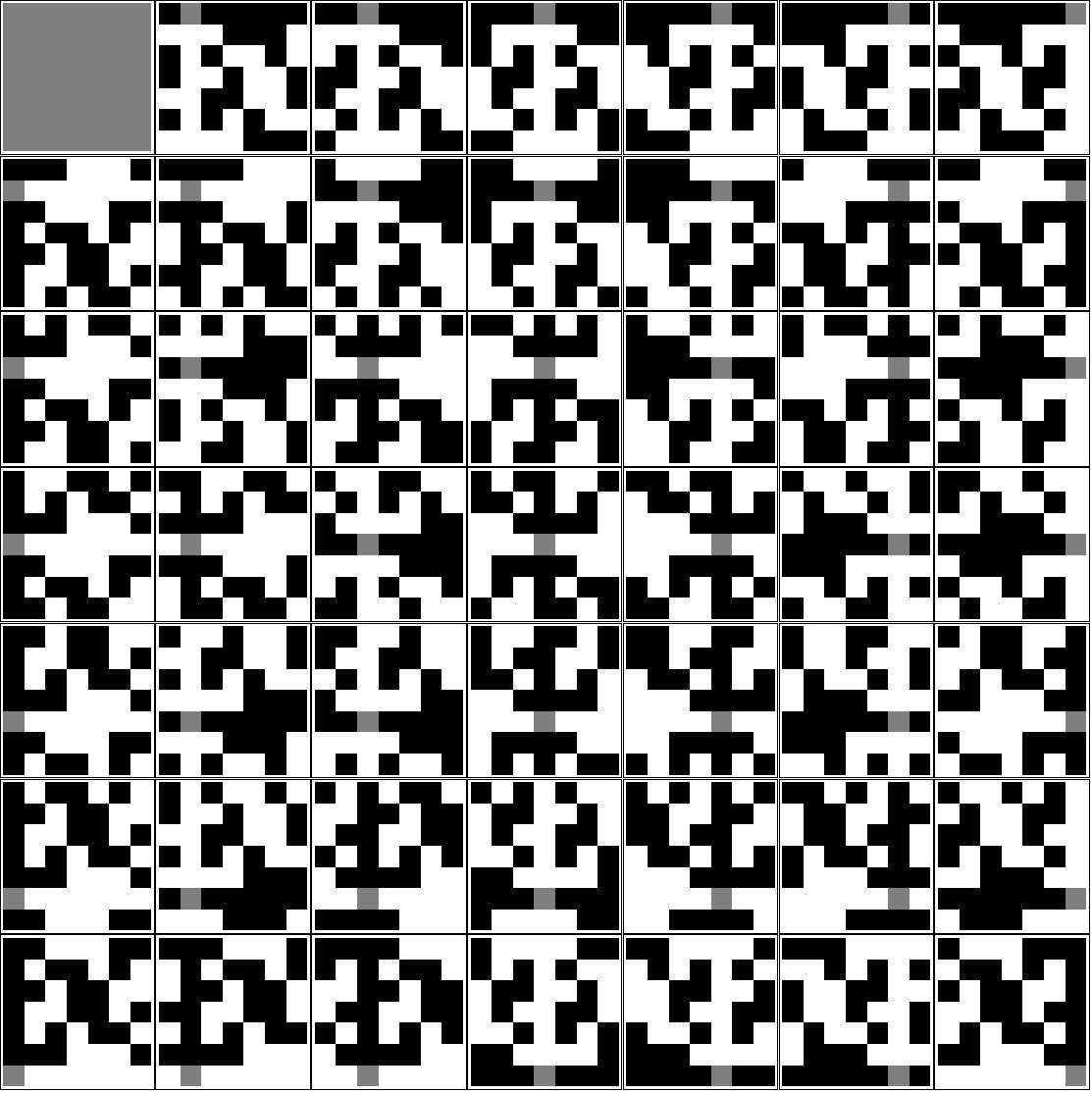
Figure 1: A plot of $\textbf{S}_{1}$ for $p=7$. ($-1$ is white, $+1$ is black and zero is gray.)

3 Watermarking imagery with higher-dimensional arrays

In this section we introduce a new application for higher-dimensional arrays with good autocorrelation and cross-correlation. We develop a new technique for embedding higher-dimensional arrays into imagery using spread spectrum watermarking techniques[16].

In the past, spread spectrum watermarking schemes used a sequence or array of dimensionality commensurate to the dimensionality of the dataset. Thus, a two-dimensional array is used to watermark an image; and every array embedded in the image supports a payload of two integers (the horizontal and vertical periodic shifts of the two-dimensional array). Then in order to support larger payloads, multiple arrays are embedded into the imagery. The embedding of multiple arrays relies on the cross-correlation properties of the families of arrays. However, even with families of optimal arrays, the signal-to-noise ratio (SNR) will decrease as more arrays are embedded.

We propose increasing the watermark payload, and subsequently increasing the SNR of the extraction, by increasing the dimensionality of the embedded arrays. We embed a $2n$-dimensional array into an image by partially flattening the array into a two-dimensional array.

We embed a $2n$-dimensional array, $\textbf{S}=\left[S_{i_{0},i_{1},\cdots,i_{2n-1}}\right]$ of size $d_{0}\times d_{1}\times\cdots\times d_{2n-1}$, into an image (2-dimensional dataset), $\textbf{I}=\left[I_{i,j}\right]$, by successively decreasing the dimensionality of S from $2n$, $\textbf{S}^{2n}$ to $n$, $\textbf{S}^{n}$, until we have a 2-dimensional array, where

$$S^{n}_{i_{0},i_{1},\cdots,i_{n}}=S^{2n}_{q_{0},q_{1},\cdots,q_{n-1},r_{0},r_{1},\cdots,r_{n-1}},$$

where $i_{0}=q_{0}d_{0}+r_{0},i_{1}=q_{1}d_{1}+r_{1},\cdots,i_{n-1}=q_{n-1}d_{n-1}+r_{n-1}$.

Example 3.1.

We convert the $4$-D array, $\textbf{S}_{1}$, from Example 2.4 into a 2-D array.

$$\left[\begin{array}[]{ccccccccc}0&0&0&1&0&1&1&1&0\\ 0&0&0&1&-1&-1&-1&1&-1\\ 0&0&0&-1&-1&1&1&-1&-1\\ 1&-1&1&1&1&-1&1&-1&-1\\ 0&-1&-1&-1&0&-1&1&1&0\\ 1&1&-1&-1&1&1&-1&1&-1\\ 1&1&-1&1&-1&-1&1&-1&1\\ 1&-1&1&-1&-1&1&-1&1&1\\ 0&-1&-1&1&0&1&-1&-1&0\\ \end{array}\right]$$

Conversely, we partition the two-dimensional image into a $2n$-dimensional representation prior to cross-correlating with the family of $2n$-dimensional arrays.

This scheme embeds $2n$ integers (as periodic shifts of the array) for each array embedded, which greatly increases the payload per array in comparison with lower-dimensional arrays.

References

• [1] S. Blake, T. E. Hall, A. Z. Tirkel, “Arrays over Roots of Unity with Perfect Autocorrelation and Good ZCZ Cross–Correlation”, Advances in Mathematics of Communications (AMC), vol. 7, no. 3, pp. 231–242, 2013
• [2] S. Blake, O. Moreno, A.Z. Tirkel, “Families of 3D Arrays for Video Watermarking”, SETA 2014, LNCS 8865, pp. 134–135, 2014
• [3] S. Blake, “Constructions for Perfect Autocorrelation Sequences and Multi-Dimensional Arrays”, PhD thesis, Monash University, April 2017
• [4] S. Blake, A. Z. Tirkel, “A Multi-Dimensional Block-Circulant Perfect Array Construction”, Advances in Mathematics of Communication, accepted for publication 2017
• [5] L. Bömer, M. Antweiler, “Construction of a new class of higher-dimensional Legendre- and pseudonoise- arrays”, IEEE Symposium on IT 90, pp. 76, San Diego, 1990
• [6] L. Bömer, M. Antweiler, H. Schotten, “Quadratic Residue Arrays”, Frequenz, vol. 47, no. 7–8, pp. 190–196, 1993
• [7] R. Gold, “Optimal binary sequences for spread spectrum multiplexing”, IEEE Trans. Inform. Theory, vol. 13, issue 4, pp. 619–621, 1967
• [8] B. Gordon, “On the existence of perfect maps”, IEEE Trans. Inform. Theory, vol. 12, issue 4, pp. 486–487, 1966
• [9] D.H. Green, “Structural Properties of Pseudo random Arrays and Volumes and their Related Sequences”, IEE Proceedings E-Computers and Digital Techniques, vol. 132, issue 3, pp. 133 – 145, 1985
• [10] D.H. Green, S.K. Amarasinghe, “Families of Sequences and Arrays with Good Periodic Correlation”, IEE Proc. E, vol. 138, issue 4, pp. 260–268, 1991
• [11] J. Jedwab, C. Mitchell, F. Piper and P. Wild, “Perfect binary arrays and difference sets”, Discr. Math., vol. 125, no. 1–3, pp. 241–254, 1994
• [12] R. Lerner, “Signals having uniform ambiguity functions”, IRE Convention Record, Information Theory Section, March 1958
• [13] A. Leukhin, O. Moreno, A. Tirkel, “Secure CDMA and Frequency Hop Sequences”, The Tenth International Symposium on Wireless Communication Systems, pp.819–825, Germany, 2013
• [14] H. D. Lüke, “Sequences and Arrays with Perfect Periodic Correlation”, IEEE Transactions on Aerospace and Electronic Systems, vol. 24, no. 3, pp. 287-294, 1988
• [15] H. D. Lüke, L. Bömer, M. Antweiler, “Perfect binary arrays”, Signal Processing, vol. 17, no. 1, pp. 69-80, 1989
• [16] A.Z. Tirkel, G.A. Rankin, R.M. Van Schyndel, W.J. Ho, N.R.A. Mee, C. F. Osborne, “Electronic Water Mark”, DICTA 93, Macquarie University, pp. 666-673, 1993
• [17] A.Z. Tirkel, C.F. Osborne, N. Mee, G.A. Rankin, A. McAndrew, “Maximal Connected Sets - Application to CDMA”, International Journal of Digital and Analog Communication Systems, vol 7, pp. 29-32, 1994
• [18] A.Z. Tirkel, C.F. Osborne and T.E. Hall, “Steganography - Applications of coding theory”, IEEE Information Theory Workshop, pp. 57–59, Norway, 1997
• [19] L. R. Welch, “Lower bounds on the maximum cross correlation of signals”, IEEE Trans. Inform. Theory, vol. 20, no. 3, pp. 603–616, May 1991
• [20] N.Y. Yu, G. Gong, “On asymptotic optimality of binary sequence families”, CACR2006-28, University of Waterloo, Canada, May 2006
• [21] N. Zierler, “Legendre Sequences”, MIT Lincoln Laboratory, Group Report 34-71, May 1958