Determination of Glass Transition Temperature of Polyimides from Atomistic Molecular Dynamics Simulations and Machine-Learning Algorithms

Abstract

Glass transition temperature ($T_{\text{g}}$) plays an important role in controlling the mechanical and thermal properties of a polymer. Polyimides are an important category of polymers with wide applications because of their superior heat resistance and mechanical strength. The capability of predicting $T_{\text{g}}$ for a polyimide a priori is therefore highly desirable in order to expedite the design and discovery of new polyimide polymers with targeted properties and applications. Here we explore three different approaches to either compute $T_{\text{g}}$ for a polyimide via all-atom molecular dynamics (MD) simulations or predict $T_{\text{g}}$ via a mathematical model generated by using machine-learning algorithms to analyze existing data collected from literature. Our simulations reveal that $T_{\text{g}}$ can be determined from examining the diffusion coefficient of simple gas molecules in a polyimide as a function of temperature and the results are comparable to those derived from data on polymer density versus temperature and actually closer to the available experimental data. Furthermore, the predictive model of $T_{\text{g}}$ derived with machine-learning algorithms can be used to estimate $T_{\text{g}}$ successfully within an uncertainty of about 20 degrees, even for polyimides yet to be synthesized experimentally.

I Introduction

When a polymer is rapidly cooled below a certain temperature, it undergoes a transition into a glassy phase where the polymer has an amorphous structure but exhibits rigidity on experimental time scales. The temperature at which this transition occurs is termed the glass transition temperature ($T_{\text{g}}$) and is one of the most important properties of a polymer that determine its performance and applications. For example, if a polymer has to stay as a hard solid in a certain application, its $T_{\text{g}}$ should be much higher than the environmental temperature, $T_{\text{e}}$. On the other hand, if a rubber or a polymer melt is required, then $T_{\text{g}}$ needs to be lower than $T_{\text{e}}$. The difference between $T_{\text{g}}$ and $T_{\text{e}}$ also strongly affects other physical properties of the polymer, such as its density and the diffusion behavior of guest gas molecules in the polymer. In other words, many physical properties of a polymer exhibit changes, which can be significant, when $T_{\text{e}}$ is varied to cross $T_{\text{g}}$. This observation is underlying a variety of methods that are used to determine $T_{\text{g}}$ via measuring or computing these physical properties as a function of temperature. The glass transition temperature is therefore a critical parameter to be considered when the target is to design or identify a polymeric material that meets the requirement of a given application. In this paper, we explore three approaches to determine $T_{\text{g}}$ for various polyimides in silico, including computing their density and gas diffusion coefficients in the polymers with atomistic molecular dynamics (MD) simulations and predicting $T_{\text{g}}$ with a model derived by applying machine-learning algorithms to analyze the existing structure-property data on $T_{\text{g}}$ of polyimides collected from literature.

Polyimides are a category of engineering plastics that have wide applications in the automotive and aerospace industries because of their relatively high $T_{\text{g}}$, high strength, and good heat resistance properties.Wilson et al. (1990); Mittal (1984) Experimentally, $T_{\text{g}}$ can be measured with differential scanning calorimetry (DSC) and thermo-mechanical analysis techniques. However, these procedures usually require careful sample preparation and control of the measurement conditions. As a supplementary approach to expedite material characterization, MD simulations have been used to quantify $T_{\text{g}}$ since the 1980s. Rigby et al. calculated $T_{\text{g}}$ for Kremer-Grest chains consisting of Lennard-Jones beads as a model of polyethylene.Rigby and Roe (1987) The temperature dependence of the polymer density, the self-diffusion coefficient, and the characteristic ratio $\langle r^{2}\rangle/(nl^{2})$ was used to identify the glass transition and $T_{\text{g}}$. Han et al. calculated $T_{\text{g}}$ for five different polymers using the curve of specific volume against temperature.Han et al. (1994) Abu-Sharkh et al. used a similar method to compute $T_{\text{g}}$ for poly(vinylchloride)s with the force field determined with an ab initio method.Abu-Sharkh (2001) In these studies, usually only one polymer chain was simulated for each system because of the limitation of computational power. Morita et al. simulated 100 coarse-grained polymer chains and introduced a method to compute $T_{\text{g}}$ by examining the mean-square displacement of a polymer segment at different temperatures.Morita et al. (2006) Buchholz et al. studied the cooling-rate-dependence of $T_{\text{g}}$ with the Kremer-Grest model, where $T_{\text{g}}$ was found from the curves of nonbonded energy or system volume versus temperature.Buchholz et al. (2002) Following these initial efforts, other researchers started to compute $T_{\text{g}}$ with atomistic MD simulations for various polymers,Fan et al. (1997); Deazle et al. (1996); Hamerton et al. (2006); Pozuelo and Baselga (2002); Hu et al. (2006); Wang et al. (2016) typically by investigating the density change of a polymer when the temperature is varied. Lyulin et al. calculated the $T_{\text{g}}$ of several polyimide polymers and pointed out that the results from MD simulations depend on cooling rate and vary if the atomistic model of a polymer considers partial charges or not.Lyulin et al. (2014a) Mohammadi et al. computed $T_{\text{g}}$ of poly(methyl methacrylate) using the first peak of the pair correlation function, the mean square displacement of polymer segments, the self-diffusion coefficient, and the internal energy of the system.Mohammadi et al. (2017) They found that though all these different physical quantities exhibit an obvious transition at $T_{\text{g}}$, the values from MD simulations are usually lower than the experimental value. All the reported work thus shows that MD simulations can be a useful tool to obtain $T_{\text{g}}$ but the results can suffer from small system sizes, short chain lengths, and high cooling rates, all reflecting the limitations of MD methods. Furthermore, the results may depend on the particular force field being used in a study.Sun et al. (2018); Alzate-Vargas et al. (2018); Luchinsky et al. (2018)

Although MD methods can be used to calculate $T_{\text{g}}$ for a polymer, the calculations can still take a long time and may be limited by available computational resources. Therefore, a predictive model of $T_{\text{g}}$ is highly desirable, which uses certain features of a polymer, such as the chemical identity of the monomer and the sequence structure of the chain, as inputs. Such a model can be applied to quickly yield $T_{\text{g}}$ that can be tested later with MD calculations or experiments. This capability will allow quick screening of a series of polymers when a particular application is in consideration. Efforts of generating so-called quantitative structure property relationships (QSPRs) for the glass transition temperature of a polymer have been ongoing since the 1990s.Sumpter and Noid (1994); Joyce et al. (1995) Joyce et al. used neural network algorithms to train a model for $T_{\text{g}}$ prediction with data on 360 monomers and the model can predict $T_{\text{g}}$ for other 89 monomers with a root mean square error (RMSE) of about 35 K.Joyce et al. (1995) The large error may be caused by the fact that the 360 monomers picked by Joyce et al. were for a broad range of polymers and with a small dataset, neural network algorithms could easily lead to overfitting. Yu et al. applied the multiple linear stepwise regression method to establish a predictive model of $T_{\text{g}}$ with a RMSE around 15.2 K.Yu et al. (2006)

Chen et al.Chen et al. (2008), Ning et al.Ning (2009), and Xu et al.Xu et al. (2012) also developed predictive models of $T_{\text{g}}$ with different accuracy for a variety of polymers. The number of data points in their training set ranges from 52 to 107. Pei et al. applied support vector regression (SVR) optimized by an integrated particle swarm optimization to predict $T_{\text{g}}$.Pei et al. (2013) They used 25 sample points to train the model and 7 other data points to test it. The RMSE of their model is around 4 K. However, the penalty factor of 56700186162.908470 used in their model training procedure is not replicable. Chen et al. applied multiple linear regression analysis to establish a predictive model of $T_{\text{g}}$ with 60 training data points.Chen et al. (2018) The test set contained 20 data points and the prediction error of $T_{\text{g}}$ was around 58 K.

Despite the existing efforts of constructing predictive models of $T_{\text{g}}$ for a range of polymers, the stability of such models has not been proved or discussed. It is unclear if the models reported in literature are robust and possess the same predictive power and accuracy if the training and test datasets are split in different ways. In this paper, we discuss the instability issue of the commonly used regularization method termed “least absolute shrinkage and selection operator” (LASSO) and find that a bragging approach can be used to enhance the stability of the predictive model of $T_{\text{g}}$ derived with LASSO. Furthermore, we compare $T_{\text{g}}$ predicted by the model trained with machine-learning algorithms with those computed with atomistic MD simulations for several polyimides that were yet synthesized at the time of prediction and computation. Later on, these polyimides were synthesized and their glass transition temperatures were measured using DSC. The predicted and computed values agree with the experimental results within 10 to 20 K. This comparison not only serves as a test of the predictive model but also validates the power of MD methods of computing $T_{\text{g}}$ for polyimides with new formulae.

This paper is organized as follows. In Sec. II, the methods of determining $T_{\text{g}}$ with atomistic MD simulations are introduced and the results are analyzed and discussed. Then in Sec. III, the procedure of building a predictive model of $T_{\text{g}}$ for polyimides using machine-learning algorithms is discussed in detail, including dataset preparation and separation, the digitization of polymer structures, the conversion of polymer structures to proper SMILES notations, the generation of polymer features from their SMILES notations, and the construction of the predictive model (i.e., the mapping from polymer features to $T_{\text{g}}$) via machine learning. Finally, conclusions are presented in Sec. IV.

II Determination of Glass Transition Temperature with All-Atom Molecular Dynamics Simulations

II.1 All-Atom Molecular Dynamics Simulation Methods

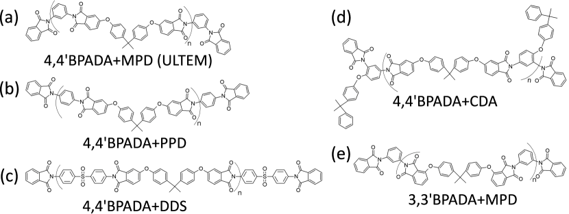
Figure 1: Structures of polyetherimides studied with all-atom MD simulations.

Atomistic MD simulations were employed previously to model the mechanical, thermal, and dielectric properties of polyetherimides.Falkovich et al. (2014); Xia et al. (2010); Luchinsky et al. (2018) The polyimide chains in our study were built with MAPS builder.Scienomics (2004-2012) In this section, 5 polyetherimides were studied, including 4,4’BPADA+MPD (ULTEM), 4,4’BPADA+PPD, 3,3’BPADA+MPD, 4,4’BPADA+CDA, and 4,4’BPADA+DDS. The chemical formulae of these polymers are shown in Fig. 1. Each chain consists of 4 repeating units (i.e., $n=4$ in Fig. 1) and the molecular weights range from 2.7 to 3.8 kDa. Phthalic anhydride (PA) groups are added to cap the chains. All MD simulations were performed using LAMMPSPlimpton (1995) with the PCFF force field.Sun et al. (1994) The equations of motion were integrated with a velocity-Verlet algorithm with time step $\Delta t=1$ fs. The Mulliken charge was included in the model and calculated using Gaussian09 software with the semi-empirical PM6 method as the basis set.Frisch et al. (2013) The cutoffs of nonbonded and Coulomb interactions were both set as 12 Å and the long-range part of Coulomb interactions was calculated using the particle-particle particle-mesh method. Each system contained 512 chains. A hydrostatic pressure of 1000 atm was used to compress the system at 300 K until it reached a density around 1.2 g/$\text{cm}^{3}$, close to the experimental value of ULTEM.Bashford (1997) Then the system was heated up to 800 K under 1 atm and equilibrated at 800 K for 5 ns. After this step, the system was gradually cooled down to 300 K under 1 atm. In this process, many configurations were created for a series of temperatures between 300 K and 800 K. At a given temperature, the corresponding configuration was taken as a starting state and the system was equilibrated further for 2 ns. The density of the polymer was then computed in a NPT ensemble with a target pressure at 1 atm controlled by a Nose-Hoover barostat. The temperature was controlled with a Nose-Hoover thermostat. The equilibrated system was also used for simulating the diffusion of gas molecules in the polymer. In these simulations, a NVT ensemble was adopted.

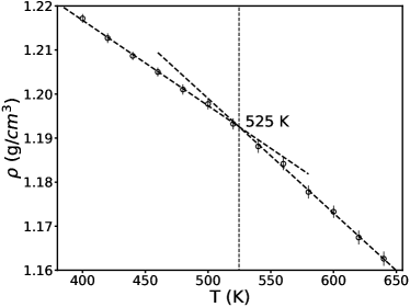
Figure 2: $\rho(T)$ vs. $T$ for 4,4’BPADA+MPD (ULTEM), for which $T_{\text{g}}=525$ K.

A commonly used protocol to determine $T_{\text{g}}$ for a polymer is to calculate its density as a function of temperature, i.e., to obtain the $\rho(T)$ curve.Yang et al. (2016); Li et al. (2009); Lyulin et al. (2014b); Minelli et al. (2012); Yoshimizu et al. (2012); Yu et al. (2001) One example is shown in Fig. 2 for ULTEM (i.e., 4,4’BPADA+MPD). The value of $T_{\text{g}}$ can be determined from the intersection of the two linear fits to $\rho(T)$, one for the lower and the other for the higher temperature region. At room temperature, the density of ULTEM from MD simulations is slightly lower than the experimental value, $1.27~{}\text{g/}\text{cm}^{3}$. The data indicate that the variation of density with temperature is captured by the PCFF force field. The value of $T_{\text{g}}$ computed from MD data on $\rho(T)$ is 525 K for ULTEM, which is 35 K higher than the experimental value, 490 K. The $\rho(T)$ curves for other polyetherimides in Fig. 1 are included in the Supporting Information. The results on their $T_{\text{g}}$ are listed in Table 1. The values determined using the $\rho(T)$ data are generally 20 to 30 K higher than the corresponding experimental values.

In addition to density, there are other properties of a polymer that can be used to determine $T_{\text{g}}$, including volume, free volume, specific volume, radial distribution functions, mean-square displacements, nonbonded energy, dihedral torsion energy, etc.Yang et al. (2016); Li et al. (2009) Many studies also showed that the diffusion behavior of gas molecules in a polymer matrix changes when the polymer undergoes a glass transition.Meares (1957); Kumins and Roteman (1961) This can be understood by examining the temperature dependence of the diffusion coefficient of a gas molecule in a polymer matrix, which has an Arrhenius form,

$$D=D_{0}~{}\text{exp}\left(-\frac{E_{A}}{RT}\right)~{},$$ (1)

where $D$ is the diffusion coefficient of the gas molecules, $D_{0}$ is a prefactor with the same unit as $D$, $E_{A}$ is the activation energy for diffusion, $T$ is the absolute temperature, and $R=8.314~{}\text{J~{}mol}^{-1}$ is the gas constant. Note that $E_{A}$ may be temperature dependent but in many cases the dependence is weak and negligible.Menzinger and Wolfgang (1969) For a glassy polymer, the value of $E_{A}$ changes when the polymer enters a glassy state from a melt state. Therefore, a plot of $D(T)$ vs. $1/T$ on a log-linear scale will show a straight line for $T>T_{\text{g}}$ and another straight line with a different slope for $T<T_{\text{g}}$. The intersections between these two lines can be used to determine $T_{\text{g}}$.

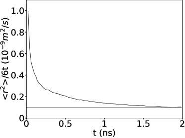
Figure 3: $\langle r^{2}\rangle/(6t)$ vs. time $t$ for argon diffusing in 4,4’BPADA+MPD (ULTEM) at 400 K, which yields $D\simeq 1.0\times{\rm 10^{-10}m^{2}/s}$.

In MD simulations, the diffusion coefficient $D$ of a gas molecule in a polymer can be computed from its mean-square displacement (MSD), $\langle r^{2}\rangle$. In the diffusive regime, its time dependence can be expressed as

$$\langle r^{2}\rangle=6Dt+C,$$ (2)

where $t$ is time and $C$ is a constant. In our simulations, 1000 inert gas atoms, either argon or neon, were added to the polymer system and their diffusion was tracked. The average MSD was then computed. One example is shown in Fig. 3, where we plot $\langle r^{2}\rangle/(6t)$ vs. $t$ for argon diffusing in 4,4’BPADA+MPD (i.e., ULTEM) at 400 K. Clearly, $\lim_{t\rightarrow\infty}\langle r^{2}\rangle/(6t)=D$. This calculation can be performed at various temperatures to generate the $D(T)$ curve. Figure 4 shows the results for argon diffusing in ULTEM, where $D$ is plotted against $1/T$ on a log-linear scale. The two regions in which $\log D$ depends $1/T$ linearly are visible. The corresponding linear fits and their intersection are used to determine $T_{\text{g}}$. For ULTEM, we find that $T_{\text{g}}\simeq 504$ K, which compared with the result determined using the $\rho(T)$ data is much closer to the experimental value (490 K). The $D(T)$ results for other polyetherimides in Fig. 1 are included in the Supporting Information.

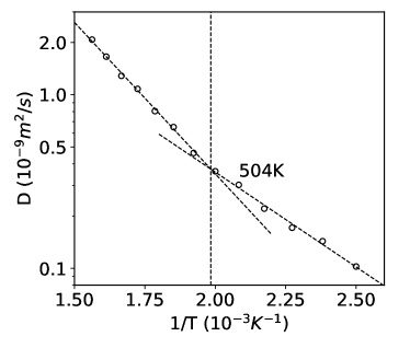
Figure 4: $D(T)$ vs. $1/T$ on a log-linear scale for argon diffusing in 4,4’BPADA+MPD (ULTEM), which yields $T_{\text{g}}=504$ K.

II.2 Molecular Dynamics Simulation Results and Discussion

Table 1: Summary of $T_{\text{g}}$ (K) for various polyetherimides from MD calculations of $\rho(T)$ and $D(T)$, the predictive model constructed using machine-learning algorithms, and DSC measurements.

	4,4’BPADA + MPD	4,4’BPADA + PPD	4,4’BPADA + DDS	4,4’BPADA + CDA	3,3’BPADA + MPD
MD [$\rho(T)$]	525	539	542	516	524
MD [$D(T)$]	504	488	532	495	500
Predicted	515	499	537	551	528
Experimental	490	unknown	520	473	511

All results on $T_{\text{g}}$ determined using either $\rho(T)$ or $D(T)$ that were computed with all-atom MD simulations are summarized in Table 1. The predicted values of $T_{\text{g}}$ by the model derived with a machine-learning approach discussed in Sec. III and the experimental results for 4 polyetherimides measured with DSC are included as well. It must be emphasized that 3 of them, including 4,4’BPADA+DDS, 4,4’BPADA+CDA, and 3,3’BPADA+MPD, were synthesized and had their $T_{\text{g}}$ measured after the computation and prediction were performed. It is noted that the values of $T_{\text{g}}$ from the $\rho(T)$ curves are generally 20 to 30 K higher than the available corresponding experimental values. However, the results on $T_{\text{g}}$ from the $D(T)$ data are closer to and only about 10 to 20 K higher than the experimental $T_{\text{g}}$’s.

The method of using gas diffusion coefficients to determine $T_{\text{g}}$ has several advantages. First of all, the results on $T_{\text{g}}$ from $D(T)$ agree better with the experimental values, as evidenced by the data in Table 1. Secondly, the diffusion coefficient of a gas molecule can be computed quickly and accurately with MD simulations. Such calculations only require fairly short MD trajectories ($\sim 1$ to 2 ns). The self-diffusion coefficient of a polymer can also be used to pinpoint $T_{\text{g}}$. However, a polymer typically diffuses much more slowly than gas molecules. As a result, much longer MD simulations are needed to compute the self-diffusion coefficient of a polymer to the same precision as in the diffusion coefficient of gas molecules. Finally, to compute $D(T)$ we can use a NVT ensemble with temperature well controlled by a suitable thermostat (e.g., a Nose-Hoover thermostat). However, to compute the $\rho(T)$ curve, a NPT ensemble is required, which needs both a thermostat and a barostat. In MD simulations, it is practically very challenging to control pressure accurately, particularly if the pressure is as small as 1 atm.Heyes (1983); Feller et al. (1995) Our MD data show that when the target pressure is 1 atm, the actual pressure in the system can fluctuate significantly from about -190 atm to about 190 atm. As a result, the polymer density also fluctuates strongly and an average over a long period of time (i.e., a long MD trajectory) is required to generate a $\rho(T)$ curve with a reasonable accuracy. Computing $D(T)$ instead of $\rho(T)$ circumvents this issue and leads a much faster convergence of the data that can be used to determine $T_{\text{g}}$, which is especially the case in the high-temperature range.

III Predictive Model of Glass Transition Temperature Trained with Machine-Learning Algorithms

III.1 Machine-Learning Methods

Machine learning is considered a subset of artificial intelligence. A machine-learning algorithm is a mathematical model that can be trained by a set of sample data without requiring the system to be explicitly programmed to generate (pre-determined) outputs on the basis of given inputs. After the training process, such a mathematical model can be used to make a future decision or prediction given new data. There are three basic machine-learning paradigms: supervised, unsupervised, and reinforcement. The process adopted here is a supervised learning method as the sample dataset used for training includes both inputs (e.g., polymer chemical identity and sequence) and desired outputs (e.g., glass transition temperature). The outcome of the learning process is an optimized objective function that connects the chemical information of a polymer, particularly its monomer type and sequence, to its measurable physical property.

Many efforts have been devoted to synthesize various polyimides, characterize their structures, and measure their properties including $T_{\text{g}}$.Fang et al. (2002); Hsiao et al. (1998); Takahashi et al. (1998); Li et al. (2003); Zhang et al. (2006) By collecting available data published in literature and applying machine-learning approaches to analyze the data, we can develop a predictive model for the glass transition temperature of polyimides. This model can be used to probe polyimides that are yet to be synthesized. In particular, in this paper we will compare the predictions of $T_{\text{g}}$ from the mapping function derived via machine learning with those computed with atomistic MD simulations for a few selected polyimides before they are made in a lab. This comparison serves as a test of the machine-learning-generated predictive model. In the future, various polyimides with potential values in terms of their performance and application will be screened with the predictive model and then selected formulae will be synthesized in a lab to validate and improve the model.

III.1.1 Database and Feature Generation

We collected 225 data points on the glass transition temperature of polyimides from literature, including 160 data points from Ref. Ding (2007) and 65 data points from Ref. Liu (2010). Some sample data are shown in Table 2. For each polymer, the chemical identity of the monomer is taken as the input. The skeleton notation of a polyimide was drawn and converted into an expression called Simplified Molecular-Input Line-Entry System (SMILES), which is a line-notation system using an ASCII string to represent the structure of a polymer. Then a feature-generating engine called E-dragon was utilized to read in the generated SMILES notations and to extract the available features for each polyimide.alv In polymer informatics, features are also called descriptors, consisting of individual measurable properties of a molecule or a polymer.Ramprasad et al. (2017); Audus and de Pablo (2017); Peerless et al. (2019) The ensemble of descriptors represents the characteristics of the polymer/molecule being studied. As polyimides are made of dianhydrides and diamines, we calculated the features for a dianhydride and a diamine group separately. For each polyimide, E-dragon generates 1342 descriptors for its dianhydride group and the same set for its diamine group. Sample features include molecular weight, sum of atomic van der Waals volumes, and sum of atomic polarizabilities, etc.

Table 2: Sample dataset of $T_{\text{g}}$ of polyimides from Refs. Ding (2007) and Liu (2010).

No.	Polyimide’s Name	SMILES Notation	$T_{\text{g}}$ (K)
1	4,4’TDPA+1,4,4APB	Nc1ccc(cc1)$\cdots$(=O)OC(=O)c7c6	234
2	3,3’ODPA+M,M’DABP	Nc1cccc(c1)$\cdots$(Oc4cccc3C(=O)OC(=O)c34)c5C6=O	234
3	4,4’ODPA+M,M’DABP	Nc1cccc(c1)$\cdots$c5ccc6C(=O)OC(=O)c6c5	235
4	3,3’ODPA+M,M’DDS	Nc1cccc(c1)$\cdots$(Oc4cccc3C(=O)OC(=O)c34)c5C6=O	241
5	3,4’TDPA+1,4,4APB	Nc1ccc(cc1)$\cdots$(Sc4ccc5C(=O)OC(=O)c5c4)c6C7=O	242
6	3,4’ODPA+M,M’DABP	Nc1cccc(c1)$\cdots$(Oc3ccc4C(=O)OC(=O)c4c3)c5C6=O	243
7	4,4’BPDA+M,M’ODA	Nc1cccc(c1)$\cdots$c6C(=O)OC(=O)c6c5	243
8	4,4’BPDA+p,p’ODA	Nc1ccc(cc1)$\dots$OC(=O)c6c5	262
9	4,4’BTDA+m,m’MDA	Nc1cccc(c1)$\dots$c5ccc6C(=O)OC(=O)c6c5	272
10	4,4’BTDA+o,o’MDA	Nc1ccc(cc1)$\dots$c7cccc6C(=O)OC(=O)c67	283
…	…	…	…

III.1.2 Data Splitting into Training Set and Test Set

For polyimides, the values of $T_{\text{g}}$ collected from Refs. Ding (2007) and Liu (2010) range from 273 K to 697 K. However, the distribution is not uniform in this range. The majority of the data is between 466 K and 583 K. The distribution of the 225 data points on $T_{\text{g}}$ is shown in Fig. 5, with a peak around 530 K. The nonuniform nature of the distribution must be considered when the dataset is split into a training set and a test set as it is important for the training set to be representative of the entire dataset. This is particularly a concern if the number of available data is limited, as in the case here. To examine the influence of how the dataset is split on the performance of the resulting predictive model of $T_{\text{g}}$, we test two different ways of dividing the dataset into a training and a test set. To this end, we only use the 160 data points from Ref. Ding (2007) to train the model and reserve the 65 data points from Ref. Liu (2010) for a completely independent test of the predictive capability of the machine-learning-trained model. To ensure that the relatively small dataset can be split consistently, we first remove the data points of $T_{\text{g}}$ at the tail of the probability distribution, i.e., those below 423 K or above 623 K. The total number of the remove data points is 9, leaving 151 points in the dataset. In the first way, this dataset is randomly split into a training set containing 85% of the data and a test set consisting of the remaining 15%. In the second way, the dataset is first divided into 8 adjoining sections, each of width of 25 K. In each section, 15% of the data points were randomly selected to join the test dataset. The remaining 85% of the data points form the training dataset. This strategy ensures that the statistical distribution of either the training or the test dataset is similar to that of the entire dataset. We designate this second approach of dividing the dataset as “statistical splitting”, while the first approach is termed “random splitting”.

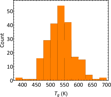
Figure 5: The distribution of $T_{\text{g}}$ of polyimides collected from Refs. Ding (2007) and Liu (2010).

III.1.3 LASSO Regularization

For a given polyimide, there were 1342 features generated for the dianhydride group and the same number of features for the diamine group. Not all these features play important roles in affecting the glass transition temperature of a polyimide. Including irrelevant or partially relevant features can lead to overfitting behavior of the resulting predictive model and negatively impact its performance. Overfitting is a common problem faced by machine-learning methods and many techniques have been developed to address this problem. In our approach, the importance of features were identified and ranked using the LASSO regularization method. At the end, a finite number of features were identified that control $T_{\text{g}}$ of polyimides.

In a linear fitting, each estimated target value $y_{i}$ could be represented as

$$y_{i}=\omega_{0}+\sum_{j=1}^{p}x_{ij}\omega_{j}+\epsilon_{i}~{},$$ (3)

where $\omega_{0}$ is a constant, $\omega_{j}$ is a fitting parameter representing the coefficient of the $j$-th feature ($x_{ij}$) in a linear mapping from features to target value, $p$ is the number of features, and $\epsilon_{i}$ is the error of predicting the $i$-th data point. In a regular linear fitting scheme, the parameters $\omega_{j}$ can be found by minimizing the error function

$$\text{error}=\sum_{i=1}^{n}(y_{i}-\omega_{0}-\sum_{j=1}^{p}x_{ij}\omega_{j})^{2}~{},$$ (4)

where $n$ is the number of data points. In the LASSO regularization method, the error to be minimized is slightly modified as

$$\text{error}=\sum_{i=1}^{n}(y_{i}-\omega_{0}-\sum_{j=1}^{p}x_{ij}\omega_{j})^{2}+\lambda\sum_{j}^{p}|\omega_{j}|~{},$$ (5)

where $\lambda$ called a penalty factor. The advantage of the LASSO regularization method is that the coefficient of irrelevant and low-importance features can be shrunk to zero, which is an effective way of removing those features. If $\lambda$ is 0, then there will no shrinkage of any of the 1342 features, and LASSO regularization becomes linear regression.Tibshirani (1996) A big positive value of $\lambda$ indicates that the majority of the features will be removed. In the LASSO regularization method, $\lambda$ is therefore called a hyper-parameter which cannot be learned directly. In our implementation, the value of $\lambda$ was exhaustively searched from 0.01 to 2.0 in increments of 0.04. Our results reveal that the typical value of $\lambda$ is between 0.3 and 1.6. For such $\lambda$, most features are removed after LASSO regularization. At the end, 197 features with nonzero coefficients remain in the final predictive model of $T_{\text{g}}$ (see the Supporting Information for the explanation of these 197 features) and the features with zero coefficients are removed during LASSO regularization. Out of 197 features, only about 12 features are actually important as indicated by their relatively large coefficients. The summation of the absolute value of coefficients of the largest 12 features is larger than the summation of the rest 185 features. Many of them can be easily justified on the basis of the available experimental evidence.

III.1.4 Bagging

Although the dataset on $T_{\text{g}}$ of polyimides has more data points than those in many previous studies on other classes of polymers,Yu et al. (2006); Chen et al. (2008); Ning (2009); Xu et al. (2012); Pei et al. (2013), it is still a small set in the perspective of machine learning. The performance of the predictive model can exhibit significant fluctuations depending on how the dataset is split into a training and a test set. To reduce such variations, we utilized a bagging approach in the learning process.Breiman (1996)

In the bagging approach, a dataset is randomly split into a training set and a test set. The machine-learning procedure described above, including the LASSO regularization method and an optimization process, is followed to generate a predictive model of $T_{\text{g}}$ using the training set. The whole process is then repeated by splitting the dataset into a new training set and a new test set. After $N_{m}$ repetitions, $N_{m}$ models are generated. The performance of each model is quantified by its error defined as

$$\text{Err}(k)=\sqrt{\frac{1}{n_{k}}\sum_{i=1}^{n_{k}}\left(T^{k}_{\text{g}}(i)_{\text{predicted}}-T^{k}_{\text{g}}(i)_{\text{target}}\right)^{2}}~{},$$ (6)

where $k$ is the index of the model and $n_{k}$ is the number of data points in the test set for the $k$-th model.

With the error associated with each model calculated, a weight, $\text{W}(k)$, was assigned to the $k$-th model according to

$$\text{W}(k)=\cfrac{\left(\text{Err}(k)\right)^{-1}}{\sum_{j=1}^{N_{m}}\left(\text{Err}(j)\right)^{-1}}.$$ (7)

The choice of the weight function in Eq. (7) guarantees that a model with a better performance, i.e., a smaller error in predicting the data in the corresponding test set, has a larger weight in the final predictive model. The final predictive model of $T_{\text{g}}$ is the linear combination of $N_{m}$ models weighted by $\text{W}(k)$ as in

$$T_{\text{g}}=\sum_{k=1}^{N_{m}}\text{W}(k)\cdot T^{k}_{\text{g}}~{}.$$ (8)

In the context of machine learning, this bagging procedure is often used to improve the robustness and stability of a learned model.

III.2 Model Training and Test

III.2.1 Various Ways of Training Predictive Model of Glass Transition Temperature

We implemented the machine-learning approach and tested the resulting predictive model of $T_{\text{g}}$ in four different ways. As discussed earlier, the dataset includes 151 data points from Ref. Ding (2007). In the first and second way, this dataset was randomly split into a test set containing 15% of the data points. The remaining 85% of the data formed the training set. In the first way, the training set was used to train the predictive model of $T_{\text{g}}$ via the LASSO regularization method but bagging was not used. In the LASSO regularization, the fitting parameter was exhaustively searched using a grid search method. The performance of the predictive model was quantified using the error of predicting the data points in the test set that never entered the training process. The entire procedure was repeated 1000 times and therefore 1000 models were generated. We analyzed the distribution of the errors of these models to predict the test set, which provided a metric quantifying the stability and performance of the first way of training the predictive model of $T_{\text{g}}$.

In the second way, “random splitting” was still used as in the first way but the bagging approach was used to train the predictive model of $T_{\text{g}}$ with each training set. In bagging, a training set was randomly split further into a training subset (85%) and a test subset (15%). The LASSO regularization method was applied to the training subset to obtain a model. This model was used to predict the test subset and the error of prediction was used to decide the weight (i.e., performance) of the model. The random splitting of the training set into two subsets was repeated 40 times, i.e., $N_{m}=40$. The linear combination of these models yielded a blended predictive model of $T_{\text{g}}$. This blended model was used to predict the test set that never entered the training process and the associated error of prediction was taken as the gauge of the model’s performance. The entire procedure was repeated 1000 times to generate 1000 blended predictive models.

The third and fourth ways were similar to the first and second ones except that “statistical splitting” discussed in Sec. III.1.2 was used instead of “random splitting”. In the third way, bagging was not used while the fourth way was a combination of “statistical splitting” and bagging. In all these ways, the first level of splitting was repeated 1000 times, resulting in 1000 models. When bagging was used, the second-level splitting of the initial training set into a training and a test subset was always repeated 40 times and therefore, all training approaches discussed here had $N_{m}=40$.

III.2.2 Performance of Predictive Model of Glass Transition Temperature

In this section, we show the performance of the predictive models of $T_{\text{g}}$ generated using the four training methods described previously. In the plots shown below, each data point represents one polyimide. For each point, the $x$-coordinate indicates the target, which is the actual value of $T_{\text{g}}$ determined experimentally. The $y$-coordinate indicates the predicted value of $T_{\text{g}}$ from a machine-learning-based model. The blue line indicates $y=x$. The closer a data point to the blue line, the better the performance of the predictive model. In Figs. 6 to 9, orange dots represent the data used in training the predictive model while the green triangles represent the data used in testing the model, which did not enter the training process.

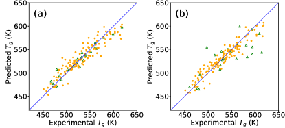
Figure 6: Performance of the (a) best and (b) worst model from training method #1 (“random splitting” + no bagging).

In our study, 1000 predictive models were generated using each training method. These models were ranked by their errors of predicting the test datasets that were not used to the model-training process. The performance of the best and worst predictive model of $T_{\text{g}}$ derived in the first manner of implementing the machine-learning approach described previously (i.e., “random splitting” + no bagging) is shown in Fig. 6. The error of using the best model to predict the training set is 14.37 K while the error is 10.78 K if the model is used to predict the test dataset. The errors of the worst model are 12.03 K for the training set and 29.62 K for the test set, respectively. The large prediction error for the test set indicates that the corresponding model has a poor prediction power.

The performance of the best and worst predictive model of $T_{\text{g}}$ trained with the second method (i.e., “random splitting” + bagging) is shown in Fig. 7. The error of predicting the training set is 14.26 K for the best model and is 12.08 K for the worst model. The best model has an error of 10.65 K when it is used to predict the test dataset while the prediction error is much larger at 29.61 K when the worst model is used.

Figure 7: Performance of the (a) best and (b) worst model from training method #2 (“random splitting” + bagging).

Figure 8 shows the performance of the best and worst models trained using the third method (i.e., “statistical splitting” + no bagging). The best model has an error of 13.65 K of predicting the training set and of 9.79 K for the test dataset. The worst model has a smaller error at 9.66 K of predicting the training set, which indicates that the model-training is successful. However, the error is much larger at 30.05 K when the test dataset was used to check the performance of the predictive model. This large discrepancy of errors of predicting the training and test dataset is a reflection of the overfitting issue faced by many machine-learning approaches. Below we show that bagging can be used to effectively address this issue.

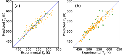
Figure 8: Performance of the (a) best and (b) worst model from training method #3 (“statistical splitting” + no bagging).

The bagging approach introduced in Sec. III.1.4 can be used to improve the stability of a machine-learning-trained predictive model. In Fig. 9, we show the performance of the best and worst model trained with the fourth method that combines “statistical splitting” of the dataset with a bagging approach. In Fig. 9(a), the errors of the best model of predicting the training and test dataset are 13.80 K and 10.21 K, respectively. For the worst model, the corresponding errors are 11.86 K and 27.37 K, as shown in Fig. 9(b).

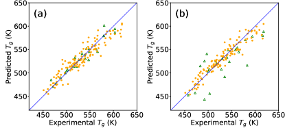
Figure 9: Performance of the (a) best and (b) worst model from training method #4 (“statistical splitting” + bagging).

To quantitatively compare the various ways of training the predictive model of $T_{\text{g}}$, we performed a statistical analysis of the errors of the 1000 models when they were used to predict the test dataset. The average and standard deviation of these errors are included in Table 3. The results show that when bagging is used, both average and standard deviation of the errors are reduced. Bagging thus enhances the stability of the machine-learning-trained model. Furthermore, the training methods in which “statistical splitting” is used to make the training dataset more statistically representative of the entire dataset also lead to predictive models with better performance. The trends indicate that the best training method is to use “statistical splitting” coupled with bagging, i.e, the fourth method.

Table 3: Performance metrics of the predictive models of $T_{\text{g}}$

Training Method	Average Error (K)	Standard Deviation of Error (K)	Correlation
Method #1	18.58	3.09	0.71
Method #2	18.31	2.98	0.84
Method #3	18.17	2.87	0.68
Method #4	17.98	2.62	0.83

In each splitting of the entire dataset into a training and a test set, a predictive model of $T_{\text{g}}$ was generated. This model is a linear mapping from all $Z$ features generated for the dianhydride and diamine groups to $T_{\text{g}}$, with the coefficient of $k$-th feature denoted as $M(k)$. A larger absolute value of $M(k)$ implies that the corresponding $k$-th feature is more strongly correlated to $T_{\text{g}}$. For two models, a correlation can thus be defined as

$$c_{ij}=\frac{2\sum^{Z}_{k=1}M_{i}(k)M_{j}(k)}{\sum^{Z}_{k=1}\left[M_{i}^{2}(k)+M_{j}^{2}(k)\right]}~{},$$ (9)

where $i$ and $j$ are the indices of the models. If the two models are identical, then $c_{ij}=1$. If the two models are anticorrelated with $M_{i}(k)=-M_{j}(k)$, then $c_{ij}=-1$. If a training method of the predictive model of $T_{\text{g}}$ is stable, then different splittings will lead to models that are highly correlated, with the correlation between the models close to 1.

We computed the correlations of all pairs out of the 1000 models generated with one of the four training methods discussed previously, using Eq. (9). The average correlation for each training method is included in Table 3. It is clear that the bagging method significantly increases the correlation between the resulting predictive models and thus enhances the stability of the training process.

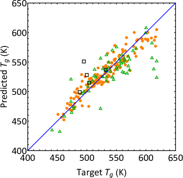
Figure 10: Performance of the predictive model of $T_{\text{g}}$ trained with 151 data points (orange dots) from Ref. Ding (2007) and tested against 63 data points (green triangles) from Ref. Liu (2010) as well as 5 polyetherimides (black squares) in Table 1. For these 5 polyetherimides, the predicted $T_{\text{g}}$ is plotted against the target value determined with $D(T)$ from all-atom MD simulations. For data from Ref. Liu (2010), the target $T_{\text{g}}$ represents the experimental value.

Finally, we used the fourth method (i.e., “statistical splitting” + bagging) to train a predictive model of $T_{\text{g}}$ with all 151 data points from Ref. Ding (2007). The model was then used to predict the 63 data points from Ref. Liu (2010). Since the training and test datasets in this case are from two different sources, this test serves as an independence check of the training method. The resulting predictive model of $T_{\text{g}}$ has an average error of 25.5 K of predicting the test set, as shown in Fig. 10. However, large errors mainly occur for high $T_{\text{g}}$ around 615 K. In the lower range of $T_{\text{g}}$, Fig. 10 indicates that the predictive model performs well in terms of predicting the independent dataset from a different source. The coefficients of all 197 features that enter the predictive model are included in the Supporting Information. Among them 12 features are found to be the most important ones. The details of these feature are also available in the Supporting Information.

We further applied the predictive model to predict $T_{\text{g}}$ for the 5 polyetherimides in Table 1. Out of this group, 4,4’BPADA+DDS, 4,4’BPADA+CDA, and 3,3’BPADA+MPD were made and characterized after the prediction. For 4,4’BPADA+PPD, the experimental values of $T_{\text{g}}$ is still unavailable as it is not synthesized yet. Therefore, we plot the predicted $T_{\text{g}}$ against the value determined with $D(T)$ from all-atom MD simulations in Fig. 10. The results show that except for 4,4’BPADA+CDA, the predictive model yields estimates close to the target values. The prediction errors are about 10 to 20 K, which are comparable to those of using the same model to predict the training dataset and even smaller than those of the independent test dataset from a different source. This comparison further validates the prediction power of the model constructed via the machine-learning approach. It also shows that a $D(T)$ curve computed with atomistic MD simulations can be used to estimate $T_{\text{g}}$ with reasonable accuracy.

IV Conclusions

In this paper we show that the PCFF force field combined with Mulliken charges can be used in all-atom MD simulations to compute and estimate $T_{\text{g}}$ of polyimides. The determination of $T_{\text{g}}$ can be achieved by computing either the polymer density, $\rho$, or diffusion coefficients of gas molecules, $D$, in the polymer matrix as a function of temperature. For temperatures lower or higher than $T_{\text{g}}$, $\rho$ exhibits a linear dependence on $T$ but the slopes are different. $D$, on the other hand, depends on $T$ as $\log D\propto 1/T$ and the linear coefficients are again different for $T<T_{\text{g}}$ and $T>T_{\text{g}}$. The comparison shows that in practice, $D$ can be more reliably computed and used to give a more accurate estimate of $T_{\text{g}}$. However, several limitations of using all-atom MD simulations to compute $T_{\text{g}}$ should be noted. First, the cooling rate used in MD simulations is typically several orders of magnitude larger than experimental rates. Secondly, the molecular weight of the polymers modeled in all-atom MD simulations is usually smaller than experimental values by a factor of 10 to 100. Thirdly, it is challenging to study a polydisperse system in MD simulations. Lastly, the PCFF force field is a generic force field for polymers and not specifically designed and optimized for polyimides. All these issues point to the need of going beyond all-atom MD simulations and seeking a predictive model that can be used to quickly estimate $T_{\text{g}}$ of polyimides.

A predictive model of $T_{\text{g}}$ of polyimides can be obtained by applying machine-learning algorithms to analyze available experimental and simulation data on $T_{\text{g}}$. We demonstrate a machine-learning approach to systematically derive such predictive models, including using a SMILES notation to designate a polymer, feature generation by reading in the SMILES notation, removal of irrelevant and low-importance features through the LASSO regularization method, and improving and optimizing the predictive models via bagging. For polyimides, we have explored 4 different training methods to construct a predictive model of $T_{\text{g}}$ of polyimides using data collected from Ref. Ding (2007) and found that the best model is obtained if the entire dataset is split into the training and test sets that are statistically representative of the entire set and if bagging is used to improve the stability of the predictive model. We further demonstrate that this model can be successfully applied to accurately predict the results on $T_{\text{g}}$ reported in Ref. Liu (2010), which were from a different source and never used to train the predictive model. Furthermore, even for polyimides that are yet to be synthesized, the predictive model yields value of $T_{\text{g}}$ close to those determined with all-atom MD simulations, which validates the prediction power of the model. In the future, it is interesting to further improve the predictive model of $T_{\text{g}}$ by training it with a larger dataset and taking into account the differences in the experimental conditions under which $T_{\text{g}}$ is measured. It is also interesting to explore if similar predictive models of other physical quantities of interest, such as dielectric constants and mechanical moduli, can be developed for polyimides.

in 1,…,25 See pages \x of SI_PEI_Tg_01-23-2020.pdf

References

- Wilson et al. (1990) D. Wilson, H. D. Stenzenberger, P. M. Hergenrother, F. W. Harris, T. Takekoshi, P. R. Young, R. Escott, H. Satou, H. Suzuki, D. Makino, et al., Polyimides (Springer, 1990).
- Mittal (1984) K. L. Mittal, ed., Polyimides: Synthesis, Characterization, and Applications, Volume 1 of the Proceedings of the First Technical Conference on Polyimides: Synthesis, Characterization and Applications (Springer US, 1984), ISBN 9780306416736.
- Rigby and Roe (1987) D. Rigby and R.-J. Roe, J. Chem. Phys. 87, 7285 (1987).
- Han et al. (1994) J. Han, R. H. Gee, and R. H. Boyd, Macromolecules 27, 7781 (1994).
- Abu-Sharkh (2001) B. F. Abu-Sharkh, Comput. Theo. Polym. Sci. 11, 29 (2001).
- Morita et al. (2006) H. Morita, K. Tanaka, T. Kajiyama, T. Nishi, and M. Doi, Macromolecules 39, 6233 (2006).
- Buchholz et al. (2002) J. Buchholz, W. Paul, F. Varnik, and K. Binder, J. Chem. Phys. 117, 7364 (2002).
- Fan et al. (1997) C. F. Fan, T. Çagin, W. Shi, and K. A. Smith, Macromol. Theo. Simul. 6, 83 (1997).
- Deazle et al. (1996) A. Deazle, I. Hamerton, C. Heald, and B. Howlin, Polymer International 41, 151 (1996).
- Hamerton et al. (2006) I. Hamerton, B. J. Howlin, P. Klewpatinond, H. J. Shortley, and S. Takeda, Polymer 47, 690 (2006), ISSN 0032-3861.
- Pozuelo and Baselga (2002) J. Pozuelo and J. Baselga, Polymer 43, 6049 (2002).
- Hu et al. (2006) N. Hu, R. Chen, and A. Hsu, Polymer International 55, 872 (2006).
- Wang et al. (2016) Y. Wang, W. Wang, Z. Zhang, L. Xu, and P. Li, Eur. Polym. J. 75, 36 (2016), ISSN 0014-3057.
- Lyulin et al. (2014a) S. V. Lyulin, S. V. Larin, A. A. Gurtovenko, V. M. Nazarychev, S. G. Falkovich, V. E. Yudin, V. M. Svetlichnyi, I. V. Gofman, and A. V. Lyulin, Soft Matter 10, 1224 (2014a).
- Mohammadi et al. (2017) M. Mohammadi, H. fazli, M. karevan, and J. Davoodi, Eur. Polym. J. 91, 121 (2017), ISSN 0014-3057.
- Sun et al. (2018) Y. Sun, L. Chen, L. Cui, Y. Zhang, and X. Du, Comput. Mater. Sci. 143, 240 (2018).
- Alzate-Vargas et al. (2018) L. Alzate-Vargas, M. E. Fortunato, B. Haley, C. Li, C. M. Colina, and A. Strachan, Model. Simul. Mater. Sci. Eng. 26, 065007 (2018).
- Luchinsky et al. (2018) D. G. Luchinsky, H. Hafiychuk, V. Hafiychuk, and K. R. Wheeler, NASA Technical Report pp. NASA/TM–2018–220213 (2018).
- Sumpter and Noid (1994) B. G. Sumpter and D. W. Noid, Macromol. Theo. Simul. 3, 363 (1994).
- Joyce et al. (1995) S. J. Joyce, D. J. Osguthorpe, J. A. Padgett, and G. J. Price, J. Chem. Soc. Faraday Trans. 91, 2491 (1995).
- Yu et al. (2006) X. Yu, X. Wang, X. Li, J. Gao, and H. Wang, Macromol. Theo. Simul. 15, 94 (2006).
- Chen et al. (2008) X. Chen, L. Sztandera, and H. M. Cartwright, International Journal of Intelligent Systems 23, 22 (2008).
- Ning (2009) L. Ning, J. Mater. Sci. 44, 3156 (2009).
- Xu et al. (2012) J. Xu, L. Zhu, D. Fang, L. Liu, W. Xu, and Z. Li, Fibers and Polymers 13, 352 (2012).
- Pei et al. (2013) J.-F. Pei, C.-Z. Cai, Y.-M. Zhu, and B. Yan, Macromol. Theo. Simul. 22, 52 (2013).
- Chen et al. (2018) M. Chen, F. Jabeen, B. Rasulev, M. Ossowski, and P. Boudjouk, J. Polym. Sci. B: Polym. Phys. 56, 877 (2018).
- Falkovich et al. (2014) S. G. Falkovich, S. V. Lyulin, V. M. Nazarychev, S. V. Larin, A. A. Gurtovenko, N. V. Lukasheva, and A. V. Lyulin, J. Polym. Sci. B: Polym. Phys. 52, 640 (2014).
- Xia et al. (2010) J. Xia, S. Liu, P. K. Pallathadka, M. L. Chng, and T.-S. Chung, Ind. Eng. Chem. Res. 49, 12014 (2010).
- Scienomics (2004-2012) Scienomics (2004-2012).
- Note (1) Note1, bPADA: 4,4’-bisphenol A dianhydride; MPD: m-phenylenediamine; PPD: para-phenylenediamine; CDA 1,2-dihydroxybenzene dianhydride: DDS: diphenyl sulfone.
- Plimpton (1995) S. Plimpton, J. Comput. Phys. 117, 1 (1995).
- Sun et al. (1994) H. Sun, S. J. Mumby, J. R. Maple, and A. T. Hagler, J. Am. Chem. Soc. 116, 2978 (1994).
- Frisch et al. (2013) M. J. Frisch, G. W. Trucks, H. B. Schlegel, G. E. Scuseria, M. A. Robb, J. R. Cheeseman, G. Scalmani, V. Barone, B. Mennucci, G. A. Petersson, et al., Gaussian 09, Revision E.01 (2013), Gaussian Inc. Wallingford CT.
- Bashford (1997) D. Bashford, in Thermoplastics (Springer, 1997), pp. 470–473.
- Yang et al. (2016) Q. Yang, X. Chen, Z. He, F. Lan, and H. Liu, RSC Adv. 6, 12053 (2016).
- Li et al. (2009) M. Li, X. Y. Liu, J. Q. Qin, and Y. Gu, Express Polym. Lett. 3, 665 (2009), ISSN 1788-618x.
- Lyulin et al. (2014b) S. V. Lyulin, S. V. Larin, A. A. Gurtovenko, V. M. Nazarychev, S. G. Falkovich, V. E. Yudin, V. M. Svetlichnyi, I. V. Gofman, and A. V. Lyulin, Soft Matter 10, 1224 (2014b), ISSN 1744-683x.
- Minelli et al. (2012) M. Minelli, M. G. De Angelis, and D. Hofmann, Fluid Phase Equilibria 333, 87 (2012), ISSN 0378-3812.
- Yoshimizu et al. (2012) H. Yoshimizu, S. Ohta, T. Asano, T. Suzuki, and Y. Tsujita, Polym. J. 44, 821 (2012), ISSN 0032-3896.
- Yu et al. (2001) K.-q. Yu, Z.-s. Li, and J. Sun, Macromol. Theory Simul. 10, 624 (2001).
- Meares (1957) P. Meares, Trans. Faraday Soc. 53, 101 (1957).
- Kumins and Roteman (1961) C. A. Kumins and J. Roteman, J. Polym. Sci. 55, 683 (1961).
- Menzinger and Wolfgang (1969) M. Menzinger and R. Wolfgang, Angew. Chem. Int. Ed. Engl. 8, 438 (1969).
- Heyes (1983) D. M. Heyes, Chem. Phys. 82, 285 (1983).
- Feller et al. (1995) S. E. Feller, Y. Zhang, R. W. Pastor, and B. R. Brooks, J. Chem. Phys. 103, 4613 (1995).
- Fang et al. (2002) X. Fang, Z. Yang, S. Zhang, L. Gao, and M. Ding, Macromolecules 35, 8708 (2002).
- Hsiao et al. (1998) S.-H. Hsiao, G.-S. Liou, and S.-H. Chen, J. Polym. Sci. A: Polym. Chem. 36, 1657 (1998).
- Takahashi et al. (1998) T. Takahashi, S. Takabayashi, and H. Inoue, High Perform. Polym. 10, 33 (1998).
- Li et al. (2003) Q. Li, X. Fang, Z. Wang, L. Gao, and M. Ding, J. Polym. Sci. A: Polym. Chem. 41, 3249 (2003).
- Zhang et al. (2006) M. Zhang, Z. Wang, L. Gao, and M. Ding, J. Polym. Sci. A: Polym. Chem. 44, 959 (2006).
- Ding (2007) M. Ding, Prog. Polym. Sci. 32, 623 (2007).
- Liu (2010) W. Liu, Polym. Eng. Sci. 50, 1547 (2010).
- (53) Molecular descriptor and fingerprint generator, https://www.alvascience.com/alvadesc/, Accessed: December 4, 2019.
- Ramprasad et al. (2017) R. Ramprasad, R. Batra, G. Pilania, A. Mannodi-Kanakkithodi, and C. Kim, npj Comput. Mater. 3, 54 (2017), ISSN 2057-3960.
- Audus and de Pablo (2017) D. J. Audus and J. J. de Pablo, ACS Macro Lett. 6, 1078 (2017).
- Peerless et al. (2019) J. S. Peerless, N. J. B. Milliken, T. J. Oweida, M. D. Manning, and Y. G. Yingling, Adv. Theo. Simul. 2, 1800129 (2019).
- Tibshirani (1996) R. Tibshirani, J. Royal Stat. Soc. B 58, 267 (1996).
- Breiman (1996) L. Breiman, Machine Learning 24, 123 (1996).