Progressive Local Filter Pruning for Image Retrieval Acceleration

Abstract

This paper focuses on network pruning for image retrieval acceleration. Prevailing image retrieval works target at the discriminative feature learning, while little attention is paid to how to accelerate the model inference, which should be taken into consideration in real-world practice. The challenge of pruning image retrieval models is that the middle-level feature should be preserved as much as possible. Such different requirements of the retrieval and classification model make the traditional pruning methods not that suitable for our task. To solve the problem, we propose a new Progressive Local Filter Pruning (PLFP) method for image retrieval acceleration. Specifically, layer by layer, we analyze the local geometric properties of each filter and select the one that can be replaced by the neighbors. Then we progressively prune the filter by gradually changing the filter weights. In this way, the representation ability of the model is preserved. To verify this, we evaluate our method on two widely-used image retrieval datasets, i.e., Oxford5k and Paris6K, and one person re-identification dataset, i.e., Market-1501. The proposed method arrives with superior performance to the conventional pruning methods, suggesting the effectiveness of the proposed method for image retrieval.

1 Introduction

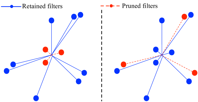
(a) Criteria for filter pruning: (left) global center-based methods, (right) our method.

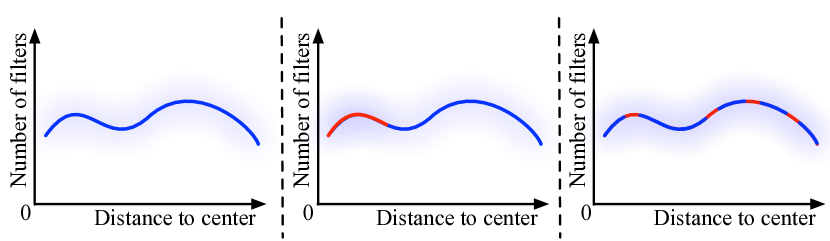
(b) Filter distributions of different methods:  (left) original filter distribution, (middle) global center-based methods, (right) our method.

Figure 1: A comparison between the conventional global center-based methods and the proposed method. In (a) the circles denote the filters, where lines denote the distance of filters to the geometric center. For global center-based methods, only the filters (with long lines) far away from the geometric center are kept, while our method prunes filters according to the local relationships to the neighbors. (b) shows the three distributions of different methods. The one generated by global center-based methods (middle) is quite different from the original filter distribution (left), while our method (right) properly maintain the original filter distribution.

Image representation learned by Convolutional Neural Network (CNN) has become dominant in image retrieval, due to the discriminative power. However, training and testing the CNN-based model usually demands expensive computation resources for the fast calculation. It remains challenging for CNN-based applications to the platforms with limited resources, e.g., cellphones and self-driving cars. To accelerate the inference, researchers resort to simplifying the CNN-based model to find a trade-off between performance and efficiency Li et al. (2016); He et al. (2017, 2018); Frankle and Carbin (2018). However, the existing network pruning methods mostly target the image classification problem. Pruning image retrieval models remains underexplored.

In this paper, we intend to fill the gap, and focus on network pruning methods for image retrieval acceleration. Compared with the image classification model, of which the output is a discrete category, the image retrieval task aims at learning continuous features. Therefore, image retrieval model is sensitive to the pruning operation in nature, which would lead to unexpected feature distribution changes. This paper addresses two main challenges in pruning image retrieval models. First, it is critical to preserve the geometry structure of filters in the original model, i.e., the filter relation of the pruned model should be the same as the original model. The existing methods mainly adopt the global center-based pruning approaches, which rank the filters according to the distance to the geometric center Li et al. (2016); He et al. (2018, 2019). However, as shown in Fig.1(b), they suffer from destroying the original filter distribution. The pruning procedure of our method and global center-based methods are illustrated in Fig. 1(a). We could observe that the global center-based methods tend to prune filters closed to the geometric center, resulting in a great change in filter distributions (Fig.1(b), middle), while our method (Fig.1(b), right) can properly maintain the original filter distributions (Fig.1(b), left).

Second, maintaining the representation ability during pruning remains challenging. The “lottery” mechanism Frankle and Carbin (2018); Sun et al. (2019) proposes to drop specific channels and argues that the key is in the weight initialization. Iterative training and rewinding is necessary for this line of methods. In this way, the models of different iterations usually have totally different feature spaces from the original model. In parallel, some pruning techniques He et al. (2018, 2019) argue that the devil is in the training process and drop the weight by deploying dynamic masks. The masks directly set the redundant filters to zeros, which also affects the learned feature space largely. In this paper, we start from a well-trained model and remove redundant filters by decreasing the weight scale gradually. It could be viewed as one mild pruning method instead of setting the filter to zeros immediately. The model representation ability, therefore, is preserved, especially for the high-proportion pruning demands.

In an attempt to overcome the above-mentioned challenges, we propose Progressive Local Filter Pruning (PLFP) to accelerate CNN models for image retrieval. 1) To maintain the distribution of the original model, we propose the local filter pruning criterion, which is different from conventional global-based criteria. The proposed method preserves the filter distribution of the original model. 2) Different from existing methods, we do not prune the model with zero masks or retrain the model from lottery initialization. Instead, we leverage the well-trained model and adopt one progressive pruning policy by changing the weight scales. To summarize, this paper has the following contributions.

• We propose to leverage the local geometric properties of the filter distribution. Thanks to the local similarity, we iteratively find the redundant filters which could be replaced by the neighbor filters. Therefore, the proposed pruning method could preserve the geometry structure of filters in the original model, even when a large proportion of filters is removed.

• As a minor contribution, we also propose a simple filter weight decreasing strategy to prune the filters progressively. Albeit simple, the progressive pruning allows the pruned model to recover the representation capability, especially when dropping a large proportion of filters. The ablation study also verifies the effectiveness of the progressing pruning.

• The extensive results on several benchmark datasets demonstrate the effectiveness of the proposed method. After reducing more than 57% FLOPs, the pruned model still achieves 76.20%, 73.18% $mAP$ on Oxford5k and Paris6k, respectively. Furthermore, we reduce 88.9% FLOPs with only 4.2% $top\text{-}5$ error increase on Market-1501.

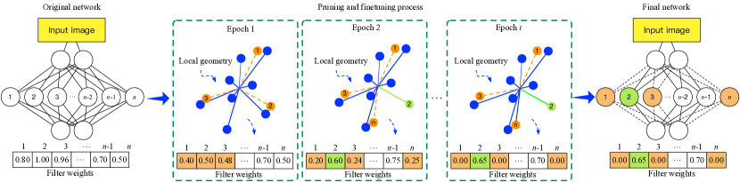
Figure 2: The geometry interpretation of the proposed method. Given a pretrained model, for a specific layer (the second layer in this example), we first calculate the local geometric properties for every filter and select redundant filters (orange filled circles) with small local power (more details are in Section 3.3). Then we deploy the filter weight decreasing policy to adjust the scale of the selected filters (orange filled squares). We iteratively re-sample candidate filters and fine-tune the model to give the wrong-selected filters chances to be rectified (green filled square), till the weight of redundant filters gradually converges to zeros. Finally, we could obtain a slim model after removing the zero-weight filters.

2 Related Work

Image Retrieval. Recently, Convolutional Neural Network (CNN) has been widely applied to extract the visual features Babenko et al. (2014); Tolias et al. (2016); Babenko and Lempitsky (2015). Babenko et al. (2014) proposes to leverage the well-trained image classification model and fine-tune the model to preserve the common knowledge for image retrieval tasks. The CNN also demands large-scale training data. Therefore, Radenović et al. (2018) proposes to utilize the 3D model to help data collection, which could greatly save the cost of manual annotation. Besides, on some sub-tasks of image retrieval, such as person re-identification Zheng et al. (2016, 2017), CNN also largely improves the preformance. Although the CNN-based feature has shown the effectiveness on the image retrieval tasks, little attention is paid to the computational cost of the image retrieval model.

Network Acceleration. There are several previous works on accelerating CNNs, such as matrix decomposition Jaderberg et al. (2014), quantization methods Gong et al. (2014); Han et al. (2015a); Rastegari et al. (2016), knowledge distillation Hinton et al. (2015); Chen et al. (2016); Kim et al. (2018), and network pruning methods He et al. (2018). Among them, pruning methods have attracted much attention as they can properly reduce computation cost and accelerate the inference by removing unnecessary filters or connections. According to the pruning policy, previous pruning methods can be roughly categorized into hard-pruning and soft-pruning methods. The early research on hard-pruning starts at the brain damage LeCun et al. (1990) and brain surgeon Hassibi et al. (1994) techniques. Han et al. (2015b) removes connections with low-weight, while Li et al. (2016) determines the importance of filters by the $l_{1}$-norm values. Another line of pruning method, soft-pruning, is a sort of training compatibility method. Soft-pruning does not drop the pruned filters immediately but utilizes a dynamic mask to set candidate filters to zeros temporally. The critical filters could be recovered later He et al. (2018). The method also could be smoothly embedded into the training framework of traditional CNN models. However, the soft-pruning methods still drop the filter via setting the weights to zeros and may largely compromise the well-trained weight from the original model, especially when pruning a large number of filters.

3 Methodology

3.1 Preliminaries

As shown in Fig. 2, we briefly illustrate the pruning process for a single convolutional layer. Our method first selects the redundant filters by the local geometry relationships. More details are provided in Section 3.2. The candidate filters are not immediately dropped. Instead, we adopt the weight decreasing policy in Section 3.3 to decrease the weight scale of selected filters. In this way, we progressively decrease the impact of the candidate filters on the network. Meanwhile, some wrong-selected filters could have chances of recovering to the original scale in the following training process.

3.2 Local Filter Selection

Formulation. We denote $W^{l}\in\mathbb{R}^{C_{out}^{l}\times C_{in}^{l}\times K^{l}\times K^{l}}$ as the weight matrix of the $l$-th convolutional layer, where $C^{l}_{out}$ and $C^{l}_{in}$ denote the number of the output channels and the input channels, respectively. $K^{l}$ is the kernel size. We intend to find redundant filters, which could be replaced by other filters. To this end, we reshape the weights $W^{l}$ as $C_{out}^{l}\times L^{l}$ with $L^{l}=C_{in}^{l}\times K^{l}\times K^{l}$. We could view the weights of the $l$-th layer $W^{l}$ as a set of filters $W^{l}=[w^{l}_{1},w^{l}_{2},\cdots,w^{l}_{C^{l}_{out}}]$, where $w^{l}_{i}$ is the $i$-th filter with the length of $L^{l}$.

Local Geometry. We intend to find redundant filters according to the mutual information. Inspired by previous works on the local manifold learning Yang et al. (2011); Li et al. (2017), which aim at locality structure exploring, we argue that the local geometry of filters could reflect more accurate mutual information. Instead of considering the relationship between all filters, we focus on the local geometry between neighbor filters. Intuitively, if one filter shares similar local properties with the neighbors, the filter could be replaced by the neighbor filters. For the $i$-th filter $w^{l}_{i}$ of the $l$-th layer, we denote the neighbor filter set as $\mathscr{N}(w^{l}_{i})$ consisting of the $k$ nearest neighbors of $w^{l}_{i}$. We could formulate the local property of the filter as:

$$\mathscr{D}(w^{l}_{i})=\frac{1}{k}\sum\limits_{w\in\mathscr{N}(w^{l}_{i})}\psi(w,w^{l}_{i}),$$ (1)

where $\psi(w,w^{l}_{i})$ denotes the distance function to model the local relationships between $w$ and $w^{l}_{i}$. Specifically, we deploy the $\mathcal{L}_{2}$ distance $\psi(w,w^{l}_{i})=||w-w^{l}_{i}||_{2}$.

Based on the previous analysis, we intend to prune filters that obtain the small local power to preserve the original filter distribution of the network. Concretely, given the pruning rate $P^{l}$ for the $l$-th layer, we want to obtain the optimal filter subset after pruning $m=P^{l}\times C^{l}_{out}$ filters. The objective could be formulated as:

$$\min\limits_{s}\sum\limits_{i=1}^{C^{l}_{out}}\bigg{(}\mathscr{D}(s_{i}w^{l}_{i})-\mathscr{D}(w^{l}_{i})\bigg{)},$$ (2)

$$s.t.\ s_{i}\in\{0,1\},\sum\limits_{i=1}^{C^{l}_{out}}s_{i}=C^{l}_{out}-m,$$

where $s$ is a filter selection vector. If $s_{i}$ equals to 1, the filter $w^{l}_{i}$ will remain, otherwise, the filter is pruned. Note that every time we change the filter selection $s$, some filters are pruned and the local neighbor relationship is also changed. To solve the Eq. (2), one naive way is to sort filters according to the local geometry distance $D(w^{l}_{(i)})$, and then select $m$ filters with the smallest local power. However, this way may lead to an elimination of filters in the most dense area. Meanwhile, the filter selection $s$ may be sub-optimal. To optimize the objective, we propose to update the filter selection in an iterative way. Specifically, we sample one filter in $W^{l}$ according to Eq. (2), re-evaluate the local power of each remaining filter, and repeat the optimization procedure till $m$ filters are sampled. If there are two or more filters obtaining the same local geometry distance. We calculate the global distance and sample the filter with the minimum global distance score. The detailed algorithm is provided in Algorithm 1.

Advantages of Local Filter Selection. The conventional pruning methods usually apply the center-based criterion, e.g., $l_{1}$-norm and Euclidean distance to the clustering center. We argue that the center-based criterion may prune the critical filters which are close to the center, and change the original filter distribution. In contrast, the proposed method focuses on keeping the filter diversity as well as preserving filter distribution of the original model. We, therefore, leverage the local geometry as the indicator to search the candidate filters. The candidates with small local power could be replaced by the near neighbors. In this way, after pruning, the model could recover the original representation capability.

Algorithm 1 Local Filter Selection

0:  The original weight $\mathcal{W}^{l}\in R^{C_{out}^{l}\times L^{l}}$, the prune rate $P^{l}$ for the $l$-th layer and the nearest neighbor number $k$.

0:  The selected filter subset $\hat{\mathcal{T}^{l}}$ with the best local power preservation.

1:  Initialize the selected subset $\hat{\mathcal{T}^{l}}\leftarrow\{\}$

2:  Initialize the rest subset $\dot{\mathcal{T}^{l}}\leftarrow\{w^{l}_{1},w^{l}_{2},\cdots,w^{l}_{C_{out}^{l}}\}$

3:  Construct an undirected graph $G=\langle V,E\rangle$ with the vertex set $V=\{w^{l}_{1},w^{l}_{2},\cdots,w^{l}_{C_{out}^{l}}\}$ and the edge set $E$ are defined as: $\forall{v_{i},v_{j}\in V,1\leq i,j\leq|V|}$, $E_{ij}\leftarrow\begin{cases}\psi(v_{i},v_{j}),&if\ i\neq j\\ 0,&\text{Otherwise}.\end{cases}$

4:  while $\arrowvert\hat{\mathcal{T}^{l}}\arrowvert<P^{l}C^{l}_{out}$ do

5:     $i^{*}=\mathop{\arg\min}_{1\leq i\leq\arrowvert\dot{\mathcal{T}}^{l}\arrowvert}\mathscr{D}(\dot{\mathcal{T}^{l}_{i}})$

6:     $\mathcal{K}=\{m|\mathscr{D}(\dot{\mathcal{T}^{l}_{m}})=\mathscr{D}(\dot{\mathcal{T}^{l}_{i^{*}}}),1\leq m\leq\arrowvert\dot{\mathcal{T}}^{l}\arrowvert\}$

7:     $j^{*}=\mathop{\arg\min}_{j\in\mathcal{K}}\sum_{i=1}^{\arrowvert\dot{\mathcal{T}^{l}}\arrowvert}E_{ji}$

8:     $\hat{\mathcal{T}^{l}}\leftarrow\hat{\mathcal{T}^{l}}\bigcup\mathcal{T}_{j^{*}}^{l}$, $\dot{\mathcal{T}^{l}}\leftarrow\dot{\mathcal{T}^{l}}-\mathcal{T}_{j^{*}}^{l}$

9:     Delete node $v_{j^{*}}$ in $V$ and the incident edges from $G$

10:  end while

11:  return  $\hat{\mathcal{T}^{l}}$

3.3 Filter Weight Decreasing

We could obtain the candidate filter subset $\hat{\mathcal{T}}^{l}$ by Algorithm 1. One way is to directly remove these filters following the hard pruning methods Li et al. (2016); Pavlo et al. (2017) by setting the corresponding filter weight to zeros. However, the operation may impact the capacity of the well-trained model, especially when a large proportion of filters is dropped. Although several soft pruning methods, e.g., He et al. (2018), propose to leverage the dynamic mask, which do not drop the filter until the training completion, the side effect caused by setting the filter to zeros also compromises the model training process. To solve this problem, we propose a simple but effective strategy to gradually reduce the value of candidate filters. Formally, for the $l$-th layer, we set the selected filters $w_{i}\leftarrow\gamma w_{i}$, where $w_{i}\in\hat{\mathcal{T}}^{l},1\leq i\leq|\hat{\mathcal{T}}^{l}|,0\leq\gamma\leq 1$. The scale of the candidate filter is decreased. Then we fine-tune the network for one epoch. The local geometry score between filters is calculated again, and we re-selected the pruned filters. In other words, the wrong-selected filters are provided more chances to recover the original scale. This ‘decreasing-fine-tune’ process is iteratively performed, till the weights of redundant filters gradually converge to zeros.

Advantages of Filter Weight Decreasing. According to the convolution operation, the filter weight decreasing actually decreases the contribution of the selected filter. For instance, the original output is $w_{i}\odot x$, and the output of the weight decreasing filter is $\gamma w_{i}\odot x$, where $\odot$ denotes the convolution operation. The contribution of the selected filter is also decreased with $\gamma$ times. If $\gamma=0$, the filter weight decreasing will equal to the conventional hard pruning methods. If $\gamma=1$, the network will not be pruned. The proposed pruning, therefore, could be viewed as one mild strategy of the hard-pruning method. We progressively decrease the contribution of the selected filters, while providing chances of recovering the wrong-selected filters. In Section 4.3, we further provide the ablation study on the effectiveness of the filter weight decreasing.

4 Experiments

We apply our pruning method on two sorts of CNN-based retrieval applications, i.e., image retrieval and personal re-identification. The following experiments are conducted with two kinds of networks, i.e., VGG-16 Simonyan and Zisserman (2015) and ResNet-50 He et al. (2016), on three benchmarks, i.e., Oxford5K Philbin et al. (2007), Paris6K Philbin et al. (2008), and Market-1501 Zheng et al. (2015).

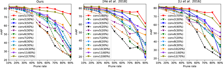
Figure 3: The pruning sensitivity of each convolutional layer for different pruning methods. The sensitive layers are marked as dashed lines and optimal prune rates for each layer are shown in figure legends. (left: Ours, middle: He et al. (2018), right: Li et al. (2016)).

4.1 Results on Personal Re-id

Experimental Setting: For the re-id application, following Zheng et al. (2019), we deploy ResNet-50 pretrained on ImageNet Deng et al. (2009) as the backbone network and replace the last average pooling layer and fully-connected layer with an adaptive max-pooling layer. We employ triplet loss function Arandjelović et al. (2018) and SGD to train the network with an initial learning rate $lr=0.001$, momentum 0.9 and the batch size of $32$. We stop training until the $100$-th epoch.

Pruning setting: Three state-of-the-art methods, i.e., He et al. (2018), He et al. (2019),  and Li et al. (2016) are introduced for comparison. Following He et al. (2018), all the convolutional layers are pruned with the same pruning rate $P$ at the same time. We test all the comparison pruning methods with $P$ from $\{10\%,20\%,50\%,90\%\}$. For soft pruning methods, i.e., He et al. (2018), He et al. (2019), and our method, we prune filters while fine-tuning for 100 epochs. For the hard pruning methods, i.e., Li et al. (2016) , to conduct a fair comparison, we prune network once and fine-tune it with the same epochs as soft pruning methods. Our method contains two hyper-parameters, i.e., $k$ and $\gamma$. We show the results with different neighbor numbers $k$ of $\{1,5,10\}$ and set $\gamma=0.01$ when $P\leqslant 50\%$ and $\gamma=0.3$ when $P>50\%$, respectively.

Results: Table 1 shows the quantitative results. We observe that our method achieves the best performance for almost all the pruning rate $P$. For example, when pruning $50\%$ filters, our method just increases the $top\text{-}5$ error 0.45%. As the pruning rate increasing, our method obtains much better results than the comparison methods. For instance, our method surpasses other methods over $8\%$ on $mAP$ and $6\%$ on $top\text{-}1$ accuracy respectively, when pruning $90\%$ filters and $88.9\%$ FLOPs have been reduced.

Table 1: Performance evaluation of the compared pruning methods on Market-1501 using ResNet-50 initialized on the Imagenet dataset.

Pruning rate(%)	Methods	mAP(%)	Rank@1(%)	Rank@5(%)	Rank@10(%)	FLOPs(%)$\downarrow$	Parameters(%)$\downarrow$
0	Zheng et al. (2019)	70.81	86.63	93.74	96.05	0	0
10	He et al. (2018)	69.08	85.45	93.85	95.78	14.50	12.92
	He et al. (2019)	70.23	86.40	93.97	95.81
	Li et al. (2016)	69.08	85.33	93.88	96.17
	Ours (k=1)	70.06	86.22	94.18	95.99
	Ours (k=5)	70.38	86.25	94.18	96.26
	Ours (k=10)	70.53	86.58	94.39	96.29
20	He et al. (2018)	69.03	84.77	93.74	95.69	28.25	24.83
	He et al. (2019)	70.07	86.07	93.79	95.81
	Li et al. (2016)	67.93	85.51	93.97	96.14
	Ours (k=1)	69.60	85.60	93.91	96.08
	Ours (k=5)	69.76	85.78	93.94	95.93
	Ours (k=10)	70.23	86.07	93.59	95.69
50	He et al. (2018)	65.85	83.05	92.96	95.52	62.45	55.57
	He et al. (2019)	65.31	83.02	91.98	94.66
	Li et al. (2016)	57.22	77.82	90.29	93.74
	Ours (k=1)	66.32	83.85	93.29	95.64
	Ours (k=5)	66.14	83.64	92.84	94.93
	Ours (k=10)	66.09	83.88	93.11	95.55
90	He et al. (2018)	48.02	71.17	86.88	90.91	88.85	74.28
	He et al. (2019)	45.31	68.26	84.74	89.64
	Li et al. (2016)	47.24	70.57	85.09	89.85
	Ours (k=1)	56.47	77.25	89.46	92.84
	Ours (k=5)	50.98	72.06	87.11	91.33
	Ours (k=10)	49.29	70.31	86.40	91.24

4.2 Results on Image Retrieval

Setting: We deploy the same backbone network, i.e., VGG-16, as Radenović et al. (2018) for image retrieval. We evaluate the pruning methods on models pretrained on the building dataset, i.e., Structure-from-Motion 3D (SfM3D) Schönberger et al. (2015). The pretrained model on SfM3D is provided by the author . We follow the conventional pipeline in Radenović et al. (2018) and extract the multi-scale representations from the images of different scale factors, i.e., $\{\frac{1}{\sqrt{2}},1,\sqrt{2}\}$. We adopt the contrastive loss function as the fine-tuning objective and use Adam Kingma and Ba (2014) to fine-tune the model with an initial learning rate $l_{0}=5\times 10^{-6}$, exponential decay $lr=l_{0}\exp{(-0.01i)}$ over epoch $i$, momentum $0.9$, margin $0.85$, and the batch size of $5$.

Pruning setting: Three state-of-the-art methods are chosen for comparison, i.e., Li et al. (2016), Pavlo et al. (2017), and He et al. (2018). Following Li et al. (2016), we investigate the pruning sensitivity of each convolutional layer and manually choose the best pruning rates (see Fig. 3). For Pavlo et al. (2017), which ranks filters through all convolution layers, we set the pruning rate to $0.4$. For our method, the hyper-parameters $k$ and $\gamma$ are set to 10 and 0.6, respectively.

Results: Table 2 summarizes the comparison results on the Oxford5K and Paris6K datasets. The proposed method arrives competitive results $76.20\%$ mAP on Oxford5K, while the $57.37\%$ FLOPs are reduced. The performance drop is limited with $-6.25\%$ mAP. Similar results are observed on Paris6K. When $61.05\%$ parameters are reduced, the pruned model still arrives a competitive performance with other pruning methods, which verifies the effectiveness of our method.

Table 2: Performance evaluation of the compared pruning methods using VGG-16 on Oxford5K and Paris6K.

Dataset	Methods	mAP(%)	FLOPs(%)$\downarrow$	Parameters(%)$\downarrow$
Oxford5K	Radenović et al. (2018)	82.45	-	-
	Li et al. (2016)	75.25	50.70	55.61
	Pavlo et al. (2017)	76.15	52.39	70.43
	He et al. (2018)	75.26	51.59	57.38
	Ours	76.20	57.37	61.05
Paris6K	Radenović et al. (2018)	81.37	-	-
	Li et al. (2016)	71.78	50.70	55.61
	Pavlo et al. (2017)	72.51	52.39	70.43
	He et al. (2018)	74.02	51.59	57.38
	Ours	73.18	57.37	61.05

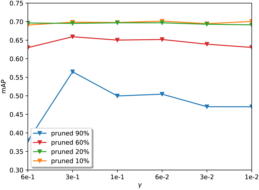
Figure 4: The parameter sensitivity analysis of our method on the Market-1501 dataset.

4.3 Parameter Sensitivity

The proposed method contains two hyper-parameters, i.e., the number of neighbors $k$ and the weight decreasing level $\gamma$. A large $k$ indicates that more neighbor filters are taken into consideration. Meanwhile, the value of $\gamma$ affects the speed of the weight decreasing.

How to determine the value of $k$ ? From Table.1, we could observe that our method is sensitive to the parameter $k$. Concretely, if $P$ is relatively small, e.g., $P\leq 20\%$, a large $k$ value will lead to a better performance. In contrast, a small $k$ value is the first choice for the high-proportion pruning demand, e.g., $P\geq 50\%$. We speculate that when a small proportion of filters is selected, a large $k$ could utilize more local information without damaging the original filter structure. When we intend to remove a large proportion of filters, the large $k$ may lead to dropping the entire points in the local geometry, which could be avoided by searching the limited local geometry. A small $k$ value, therefore, performs well in this condition. Only the closest neighbor is taken into consideration.

The effect of weight decreasing. To study the importance of parameter $\gamma$, we evaluate different $\gamma$ values from $\{0.6,0.3,0.1,0.06,0.03,0.01\}$ on the Market-1501 dataset under different pruning rates $P$ varying from $\{10\%,20\%,60\%,90\%\}$. We fix $k=1$ in the ablation study. The results are shown in Fig. 4. We observe that our method is not sensitive to $\gamma$ when $P$ is small, e.g., $P=10\%~{}\text{and}~{}P=20\%$. In contrast, when a large proportion of parameters is dropped, e.g., $P>50\%$, the larger $\gamma$ significantly performs well, which decreases the filter scale slowly. It is consistent with our intuition that the filter weight decreasing helps the model to adapt to the large prune rate. Note that if the value of $\gamma$ is too large, e.g., $\gamma=0.6$, the network may converge very slowly, and limited filters are decreased to zeros. To compare the results fairly, we use the hard-pruning method to drop the final weights, so the model of $\gamma=0.6$ does not perform well.

4.4 Feature Map Visualization

To explore the effectiveness of the proposed method, we further visualize the first convolutional layer feature maps shown in Fig. 5, where we have pruned 10% of filters and marked the corresponding feature maps with red boxes. These pruned feature maps contain the outlines of the input image, such as straps (2, 31), T-shirts (13, 59), shorts (28), and hat (57). Clearly, these feature maps can be replaced by the remaining ones. For example, straps, T-shirts, shorts, and hats can be replaced by feature maps: (43, 54, 55, et al.), (11, 42,  et al.), (20, 22  et al.), and (1, 34, 53,  et al.) respectively.

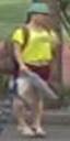
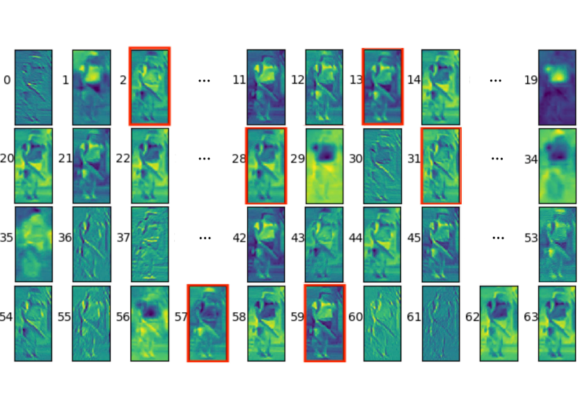
Figure 5: The input image (left) and the visualization of the first convolutional layer feature maps (indexed from 0 to 63) (right). The maps with red boxes are pruned by our method.

4.5 Embedding Feature Analysis

Table 3: The mean Euclidean distance on Market-1501 between the embedding features extracted from the original model and the pruned models with different pruning methods.

Methods	Distance ( $\times 10^{-2}$)	mAP(%)
He et al. (2019)	35.28	45.31
Li et al. (2016)	35.17	47.24
He et al. (2018)	35.13	48.02
Ours ($k=1$)	34.70	56.47

As mentioned above, maintaining the original filter distribution of the network is critical for image retrieval. To study it, we compute the Euclidean distance between the embedding features of the original model and pruned models with 90% filters removed. Our model extracts the most similar features with the baseline model, which indicates that the proposed method is suitable for pruning image retrieval networks.

5 Conclusion

This paper has proposed a progressive local filter pruning strategy for image retrieval acceleration. Different from the existing global center-based pruning methods, our method seeks to reduce filter redundancy by considering the local relations of filters. Furthermore, the filter weight decreasing allows the pruned model to recover the representation capability, especially when dropping a large proportion of filters. Compelling results on computation reduction and feature representation maintaining demonstrate the effectiveness of our method.

References

- Arandjelović et al. [2018] R. Arandjelović, P. Gronat, A. Torii, T. Pajdla, and J. Sivic. Netvlad: Cnn architecture for weakly supervised place recognition. TPAMI, 2018.
- Babenko and Lempitsky [2015] Artem Babenko and Victor S. Lempitsky. Aggregating local deep features for image retrieval. ICCV, 2015.
- Babenko et al. [2014] Artem Babenko, Anton Slesarev, Alexander Chigorin, and Victor S. Lempitsky. Neural codes for image retrieval. abs/1404.1777, 2014.
- Chen et al. [2016] Tianqi Chen, Ian Goodfellow, and Jonathon Shlens. Net2net: Accelerating learning via knowledge transfer. In ICLR, 2016.
- Deng et al. [2009] J. Deng, W. Dong, R. Socher, L. Li, Kai Li, and Li Fei-Fei. Imagenet: A large-scale hierarchical image database. In CVPR, 2009.
- Frankle and Carbin [2018] Jonathan Frankle and Michael Carbin. The lottery ticket hypothesis: Training pruned neural networks. CoRR, abs/1803.03635, 2018.
- Gong et al. [2014] Yunchao Gong, Liu Liu, Ming Yang, and Lubomir D. Bourdev. Compressing deep convolutional networks using vector quantization. abs/1412.6115, 2014.
- Han et al. [2015a] Song Han, Huizi Mao, and William J. Dally. Deep compression: Compressing deep neural network with pruning, trained quantization and huffman coding. abs/1510.00149, 2015.
- Han et al. [2015b] Song Han, Jeff Pool, John Tran, and William J. Dally. Learning both weights and connections for efficient neural networks. abs/1506.02626, 2015.
- Hassibi et al. [1994] Babak Hassibi, David G. Stork, and Gregory Wolff. Optimal brain surgeon: Extensions and performance comparisons. In NeurIPS. 1994.
- He et al. [2016] K. He, X. Zhang, S. Ren, and J. Sun. Deep residual learning for image recognition. In CVPR, 2016.
- He et al. [2017] Yihui He, Xiangyu Zhang, and Jian Sun. Channel pruning for accelerating very deep neural networks. ICCV, 2017.
- He et al. [2018] Yang He, Guoliang Kang, Xuanyi Dong, Yanwei Fu, and Yi Yang. Soft filter pruning for accelerating deep convolutional neural networks. In IJCAI, 2018.
- He et al. [2019] Yang He, Ping Liu, Ziwei Wang, Zhilan Hu, and Yi Yang. Filter pruning via geometric median for deep convolutional neural networks acceleration. In CVPR, 2019.
- Hinton et al. [2015] Geoffrey Hinton, Oriol Vinyals, and Jeffrey Dean. Distilling the knowledge in a neural network. In NIPS Deep Learning and Representation Learning Workshop, 2015.
- Jaderberg et al. [2014] Max Jaderberg, Andrea Vedaldi, and Andrew Zisserman. Speeding up convolutional neural networks with low rank expansions. In BMVC, 2014.
- Kim et al. [2018] Jangho Kim, Seonguk Park, and Nojun Kwak. Paraphrasing complex network: Network compression via factor transfer. In NeurIPS. 2018.
- Kingma and Ba [2014] Diederik P Kingma and Jimmy Ba. Adam: A method for stochastic optimization. arXiv:1412.6980, 2014.
- LeCun et al. [1990] Yann LeCun, John S. Denker, and Sara A. Solla. Optimal brain damage. In NeurIPS. 1990.
- Li et al. [2016] Hao Li, Asim Kadav, Igor Durdanovic, Hanan Samet, and Hans Peter Graf. Pruning filters for efficient convnets. abs/1608.08710, 2016.
- Li et al. [2017] Xuelong Li, Mulin Chen, Feiping Nie, and Qi Wang. Locality adaptive discriminant analysis. In IJCAI, 2017.
- Pavlo et al. [2017] Molchanov Pavlo, Tyree Stephen, Karras Tero, Aila Timo, and Kautz Jan. Pruning convolutional neural networks for resource efficient inference. ICLR, 2017.
- Philbin et al. [2007] J. Philbin, O. Chum, M. Isard, J. Sivic, and A. Zisserman. Object retrieval with large vocabularies and fast spatial matching. In CVPR, 2007.
- Philbin et al. [2008] J. Philbin, O. Chum, M. Isard, J. Sivic, and A. Zisserman. Lost in quantization: Improving particular object retrieval in large scale image databases. In CVPR, 2008.
- Radenović et al. [2018] F. Radenović, G. Tolias, and O. Chum. Fine-tuning CNN image retrieval with no human annotation. TPAMI, 2018.
- Rastegari et al. [2016] Mohammad Rastegari, Vicente Ordonez, Joseph Redmon, and Ali Farhadi. Xnor-net: Imagenet classification using binary convolutional neural networks. In ECCV, 2016.
- Schönberger et al. [2015] Johannes L. Schönberger, Filip Radenović, Ondřej Chum, and Jan-Michael Frahm. From single image query to detailed 3d reconstruction. CVPR, 2015.
- Simonyan and Zisserman [2015] Karen Simonyan and Andrew Zisserman. Very deep convolutional networks for large-scale image recognition. In ICLR, 2015.
- Sun et al. [2019] Tianxiang Sun, Yunfan Shao, Xiaonan Li, Pengfei Liu, Hang Yan, Xipeng Qiu, and Xuanjing Huang. Learning sparse sharing architectures for multiple tasks. AAAI, 2019.
- Tolias et al. [2016] Giorgos Tolias, Ronan Sicre, and Hervé Jégou. Particular Object Retrieval With Integral Max-Pooling of CNN Activations. In ICLR, 2016.
- Yang et al. [2011] Yi Yang, Heng Tao Shen, Zhigang Ma, Zi Huang, and Xiaofang Zhou. L2,1-norm regularized discriminative feature selection for unsupervised learning. In IJCAI, 2011.
- Zheng et al. [2015] L. Zheng, L. Shen, L. Tian, S. Wang, J. Wang, and Q. Tian. Scalable person re-identification: A benchmark. In ICCV, 2015.
- Zheng et al. [2016] Liang Zheng, Yi Yang, and Alexander G. Hauptmann. Person re-identification: Past, present and future. CoRR, abs/1610.02984, 2016.
- Zheng et al. [2017] Zhedong Zheng, Liang Zheng, and Yi Yang. A discriminatively learned cnn embedding for person reidentification. ACM TOMM, 2017.
- Zheng et al. [2019] Zhedong Zheng, Xiaodong Yang, Zhiding Yu, Liang Zheng, Yi Yang, and Jan Kautz. Joint discriminative and generative learning for person re-identification. CVPR, 2019.