Simple and Effective Prevention of Mode Collapse in Deep One-Class Classification

Abstract

Anomaly detection algorithms find extensive use in various fields. This area of research has recently made great advances thanks to deep learning. A recent method, the deep Support Vector Data Description (deep SVDD), which is inspired by the classic kernel-based Support Vector Data Description (SVDD), is capable of simultaneously learning a feature representation of the data and a data-enclosing hypersphere. The method has shown promising results in both unsupervised and semi-supervised settings. However, deep SVDD suffers from hypersphere collapse—also known as mode collapse—, if the architecture of the model does not comply with certain architectural constraints, e.g. the removal of bias terms. These constraints limit the adaptability of the model and in some cases, may affect the model performance due to learning sub-optimal features. In this work, we consider two regularizers to prevent hypersphere collapse in deep SVDD. The first regularizer is based on injecting random noise via the standard cross-entropy loss. The second regularizer penalizes the minibatch variance when it becomes too small. Moreover, we introduce an adaptive weighting scheme to control the amount of penalization between the SVDD loss and the respective regularizer. Our proposed regularized variants of deep SVDD show encouraging results and outperform a prominent state-of-the-art method on a setup where the anomalies have no apparent geometrical structure.

I Introduction

Anomaly detection [1] has long been an active area of research [2, 3]. It refers to the detection of unusual events or instances in the data that do not conform to the normal behavior [1]. Anomaly detection algorithms are used extensively in a wide range of applications such as network intrusion detection systems [4], fraud detection systems [5], and the detection of cyber attacks in Cyber-Physical systems (CPS) [6]. In principal, one can frame anomaly detection as a binary supervised classification problem, but such an approach has several disadvantages. An algorithm which learns to classify directly the normal versus anomalous samples has no guarantee to generalize well to new types of anomalies or threats. It is also challenging to collect all possible types of anomalies/threats due to their diversity, lack of labels, or the cost to obtain. Addressing this, Steinwart et al. (2005) [7] assume a uniform distribution for anomalous points, but their approach suffers from the curse of dimensionality. To detect new anomalies, many of these systems adopt an unsupervised learning approach as foundation for their detection algorithm. Some approaches involve detection based on reconstruction errors [8, 9] and some are based on principles derived from classification approaches [10, 11, 12].

Recently [13] proposed an unsupervised one-class classification approach—deep SVDD, which jointly learns the feature representation of the data and a data-enclosing hypersphere. The unsupervised deep SVDD model has been generalized to a semi-supervised deep SVDD model [14]. However, both models suffer from hypersphere collapse if the architecture of the model does not comply with a set of architectural constraints. The imposed set of constraints include the use of only unbounded activation functions and the removal of bias terms in the network architecture [13]. Imposing these restrictions may cause the network to learn sub-optimal features only. A conceptually related problem to hypersphere collapse is the mode collapse problem observed in GANs [15, 16]. In GANs, the generated samples tend to collapse to a limited number of modes without proper regularization. In the case of deep SVDD, the learned features collapse to a single point if the architectural constraints are not enforced. We use the two terms—mode and hypersphere collapse—interchangeably in this work. We provide related work on the mode collapse problem in GANs in Section II.

In this paper, we address the hypersphere collapse problem in deep SVDD as follows. We propose two regularizers based on random noise injections and minibatch variance, respectively. The resulting regularized variants of deep SVDD form a simple, yet effective regularization against hypersphere collapse in deep SVDD, thereby allowing the removal of architectural constraint on the bias term and activation. The following summarizes our contributions in this work.

1. We propose a regularization technique against hypersphere collapse based on noise injection via the standard cross-entropy loss.

2. We propose a regularization technique against hypersphere collapse that penalizes the minibatch variance if it falls below some annealed threshold.

3. We propose an adaptive weighting scheme to control the balance between the deep SVDD loss and the regularizer.

4. We show that our regularized deep SVDD variants generally perform better than the standard deep SVDD and other methods for both unsupervised and semi-supervised settings.

II Related Work

Anomaly detection.  Approaches in this area can be broadly divided into reconstructive and classification-based methods. For reconstructive methods, usually with autoencoders or GANs, anomalies can be detected from analysing the reconstruction errors since the model only learns to reconstruct normal samples during training. In [8], the authors proposed the robust deep autoencoders (RDA) method which is a combination of autoencoders and robust principle component analysis (RPCA) [17] for anomaly detection. A more advanced approach [18] handles the dataset contamination problem by adapting an adversarial autoencoder architecture to impose a prior distribution on the latent representation by placing anomalies into low likelihood-regions. On the other hand, the authors in [9] are the first to employ a GAN approach for anomaly detection. They introduce the unsupervised AnoGAN model to learn a manifold of the normal samples with generative and discriminative components. Other works that adopt GANs for anomaly detection are [19, 20, 21].

Another class of anomaly detection algorithms are classification-based approaches. The isolation forest (IF) [12] and the one-class support vector machine (OC-SVM) [10] are unsupervised methods. The kernel-based SVDD [11] which learns a data-enclosing hypersphere of a minimum volume in feature space is inspired by the OC-SVM. The deep SVDD model [13] improves the kernel-based SVDD model by simultaneously learning the feature representation of the unlabeled data and the minimum volume data-enclosing hypersphere. The unsupervised deep SVDD method has also been generalized to the semi-supervised setting [14]. In [22], the authors learn to solve the auxiliary task of classifying different geometric transformations of the normal data. The anomalies are then identified based on their softmax activation statistics of the transformed images. Their approach achieves a new state-of-the-art performance on the CIFAR10 dataset, significantly outperforming some prominent reconstruction and classification-based approaches, including the standard deep SVDD model [13].

Mode collapse in GANs.  The hypersphere collapse problem in deep SVDD is conceptually similar to the mode collapse problem in GANs. Deep generative models such as GANs, are known to be difficult to train, unstable, and prone to mode collapse [15, 16]. Without proper regularization, the generator often collapses and thus, generates only samples of a few modes or a single mode of class. In [23], the authors argue that the training issues in GANs are due to the lack of control over the discriminator, and the naturally disjoint manifolds of the actual and generated data. They add a mode regularizer to the generator’s optimization target in an attempt to encourage the generated samples to move towards a nearby mode of the data generating distribution. On the other hand, [16] introduces a set of training methods such as the minibatch discrimination method to improve the training of GANs. Subsequently, [24] proposes an additional reconstructor network that learns to map from the input data distribution to Gaussian random noise. By training the generator and reconstructor networks simultaneously via an implicit variational principle in VEEGAN, the reconstructor network learns the mapping from the data distribution to Gaussian and an approximate inverse of the generator, thereby preventing mode collapse. The work [25] proposes a latent-space constraint loss to prevent mode collapse in Boundary Equilibrium Generative Adversarial Network (BEGAN) [26].

In this work, we compare our proposed regularized variants of deep SVDD with the state-of-the-art method [22] as well as other classification-based anomaly detection methods.

III Preliminaries

Deep SVDD [13, 14] is an extension of the kernel-based SVDD method [11]. The kernel-based SVDD learns a data-enclosing hypersphere of minimum volume in feature space from the unlabeled training data. However, the kernel method requires manual feature engineering and scales poorly due to the computation/manipulation of the kernel matrix. Deep SVDD overcomes these limitations by jointly learning a suitable feature representation of the data and mapping them to a minimum volume hypersphere [13, 14]. Nonetheless, under certain conditions, deep SVDD is not fully robust against mode collapse, which will be elaborated in Section VI.

III-A Unsupervised Deep SVDD

For some input space $\mathcal{X}\subseteq\mathbb{R}^{d}$ and output space $\mathcal{F}\subseteq\mathbb{R}^{p}$, let $\phi(\cdot\ ;\mathcal{W}):\mathcal{X}\rightarrow\mathcal{F}$ be a neural network with $L$ hidden layers and a set of weights $\mathcal{W}=\{W^{1},...,W^{L}\}$ where $W^{l}$ are the weights of layer $l\in\{1,...,L\}$. Therefore, $\phi(x;\mathcal{W})\in\mathcal{F}$ is the feature representation of $x\in\mathcal{X}$. Unsupervised deep SVDD jointly learns the feature representation and minimizes the volume of a hypersphere in $\mathcal{F}$. Given the unlabeled training data $\mathcal{D}_{n}=\{x_{1},...,x_{n}\}$, the soft-boundary objective function is given as

$$\min_{\mathcal{R,W}}R^{2}+\frac{1}{\nu n}\sum^{n}_{i=1}\max\{0,||\phi(x_{i};\mathcal{W})-c||^{2}-R^{2}\}\\ +\frac{\lambda}{2}\sum^{L}_{l=1}||W^{l}||^{2}_{F}\ \$$ (1)

where $R$ is the radius, $c\in\mathcal{F}$ is the center of the hypersphere, and $\nu\in(0,1]$ is the trade-off between the volume and boundary violations of the hypersphere, i.e. fraction of outliers. $c$ is fixed as the mean of the mapped data from an initial forward pass [13]. For every iteration, $R$ is computed as the $(1-\nu)$-th quantile of $||\phi(x_{i};\mathcal{W})-c||_{2}$. Assuming most of the training data is normal, objective (1) can be simplified to the following one-class objective function

$$\min_{\mathcal{W}}\frac{1}{n}\sum^{n}_{i=1}||\phi(x_{i};\mathcal{W})-c||^{2}+\frac{\lambda}{2}\sum^{L}_{l=1}||W^{l}||^{2}_{F}.$$ (2)

III-B Semi-supervised Deep SVDD

In the semi-supervised approach, the model has access to both unlabeled training samples $x_{1},...,x_{n}\in\mathcal{X}$, and labeled training samples $(\tilde{x}_{1},\tilde{y}_{1}),...,(\tilde{x}_{m},\tilde{y}_{m})\in\mathcal{X}\times\mathcal{Y}$, where $\mathcal{X}\subseteq\mathbb{R}^{d}$ and $\mathcal{Y}=\{-1,+1\}$. Normal samples are labeled as $\tilde{y}=+1$ and anomalies as $\tilde{y}=-1$. The one-class semi-supervised Deep SVDD objective function is formulated as

$$\min_{\mathcal{W}}\frac{1}{n+m}\sum^{n}_{i=1}||\phi(x_{i};\mathcal{W})-c||^{2}\\ +\frac{\eta}{n+m}\sum^{m}_{j=1}(||\phi(\tilde{x}_{j};\mathcal{W})-c||^{2})^{\tilde{y}_{j}}.$$ (3)

We omitted the weight decay regularizer in the above formulation for simplicity. For more information, we refer the reader to the work [13, 14].

IV Proposed Methodology

The hypersphere collapse phenomenon and the architectural constraints for deep SVDD are briefly described in Section IV-A. The two different regularization methods are presented in Section IV-B and Section IV-C, respectively. Section IV-D discusses the adaptive weighting scheme used to control the scaling between the deep SVDD loss and the respective regularizer.

IV-A Hypersphere Collapse

According to [13, 14], an improperly formulated deep SVDD network (which includes the hypersphere center $c$), may lead to the learning of a trivial solution, i.e. hypersphere/mode collapse, a phenomenon where the features learned by the network converge to a single point, $\phi\equiv c$. It has been recommended that the center $c$ must be something other than the all-zero-weights solution, and the network should use only unbounded activations and omit bias terms to avoid a hypersphere collapse. However, omitting bias terms in a network may only lead to a sub-optimal feature representation due to the role of bias in shifting activation values. In this work, we propose two simple regularization techniques against mode collapse in deep SVDD which allow the revoke of previous restrictions on the class of networks.

IV-B Regularization with Random Noise Injection via the Loss Layer

We revisit the timeless idea of noise injection in machine learning, and, inspired by methods which address the overfitting issue in convolutional neural networks (CNNs) [27, 28], we took a similar regularization approach for a loss layer to prevent mode collapse in deep SVDD. We added a new loss layer on top of the feature extractor to learn $k$ randomly labeled classification tasks in conjunction with the SVDD objective function. For some input space $\mathcal{X}\subseteq\mathbb{R}^{d}$, feature space $\mathcal{F}\subseteq\mathbb{R}^{p}$, and output space $\mathcal{K}\subseteq\mathbb{R}^{k}$, let $\phi(\cdot\ ;\mathcal{W}_{0}):\mathcal{X}\rightarrow\mathcal{F}$ be a neural network with $L$ hidden layers, and $g(\cdot\ ;\mathcal{W}_{1}):\mathcal{F}\rightarrow\mathcal{K}$ be the linear layer after it. The final network is given by $z(x;\mathcal{W})=g(\phi(x;\mathcal{W}_{0});\mathcal{W}_{1})\in\mathcal{K}$, where $\phi(x;\mathcal{W}_{0})\in\mathcal{F}$ is the feature representation of $x\in\mathcal{X}$. For a given input sample $x_{i}$, we define $z_{i,q}$ as the $q$-th element of the $k$-dimension logits vector $z(x_{i};\mathcal{W})$ and $\sigma$ as the sigmoid function. We add the following sigmoid cross-entropy loss as a regularizer to the standard unsupervised or semi-supervised deep SVDD loss $\mathcal{L}_{SVDD}$ (Eq. (1), (2) or (3)).

$$\mathcal{L}_{reg}=-\frac{1}{nk}\sum^{n}_{i=1}\sum^{k}_{q=1}y_{rnd}\log\sigma(z_{i,q})\\ +(1-y_{rnd})\log(1-\sigma(z_{i,q})).$$ (4)

This approach is based on the idea that learning a single classification problem with meaningful, non-random labels would prevent mode collapse orthogonal to the decision boundary. Therefore, when given random binary labels, the classifier aims at preventing mode collapse along a randomly varying set of hyperplanes, which may potentially lead to better convergence. Here, at each iteration, the binary labels $y_{rnd}$ are randomly sampled from the uniform distribution of $\{0,1\}$ for each sample. At test time, the linear layer $g(\cdot\ ;\mathcal{W}_{1})$ will be removed. We present the overall loss function used in the training of the regularized deep SVDD in Section IV-D.

IV-C Regularization with Hinge Loss on Minibatch Variance

We also consider using the hinge loss [29] to penalize the minibatch variance if it falls below a specified threshold. This ensures the features in a minibatch to differ sufficiently, thereby preventing mode collapse. Being able to specify the threshold also gives us more control over the regularization as compared to the method presented in Section IV-B which is based on random noise injection. Using the notations from Section IV-B, we define $\phi_{i,q}$ as the $q$-th feature from the feature vector $\phi(x_{i};\mathcal{W}_{0})\in\mathcal{F}$ of the input sample $x_{i}$. We do not add a linear layer after the feature extractor $\phi(\cdot\ ;\mathcal{W}_{0})$ as done in Section IV-B. We add the following regularization loss to the standard unsupervised or semi-supervised deep SVDD loss $\mathcal{L}_{SVDD}$ (Eq. (1), (2) or (3)).

$$\mathcal{L}_{reg} =\max\{0,d_{\tilde{t}}-\frac{1}{p(n-1)}\sum_{q=1}^{p}\sum_{i=1}^{n}(\phi_{i,q}-\overline{\phi}_{q})^{2}\}$$ (5)

$$=\max\{0,d_{\tilde{t}}-\frac{1}{p(n-1)}\sum_{q=1}^{p}\sum_{i=1}^{n}(\phi_{i,q}-\frac{1}{n}\sum_{k=1}^{n}\phi_{k,q})^{2}\}.$$

The term $\frac{1}{p(n-1)}\sum\limits_{q=1}^{p}\sum\limits_{i=1}^{n}(\phi_{i,q}-\overline{\phi}_{q})^{2}$ computes the sample variance of the minibatch of features averaged over $p$ dimensions (the dimension of the feature vector) and $d_{\tilde{t}}$ refers to the variance threshold used for penalization at epoch $\tilde{t}$. This formulation enforces a penalty only when the minibatch variance falls below the threshold, i.e. $\frac{1}{p(n-1)}\sum\limits_{q=1}^{p}\sum\limits_{i=1}^{n}(\phi_{i,q}-\overline{\phi}_{q})^{2}<d_{\tilde{t}}$. We circumvent the general problem of selecting an appropriate variance threshold with an annealing approach that gradually decreases the threshold $d_{\tilde{t}}$ by a factor of $10$ every $r$ epochs. The overall loss function used in the training of the regularized deep SVDD will be discussed in the next sub-section.

IV-D Adaptive Weighting Scheme

We minimize the following objective function for the regularized variant of deep SVDD.

$$\mathcal{L}_{final}=\mathcal{L}_{SVDD}+c_{t}\cdot\mathcal{L}_{reg},$$ (6)

where $c_{t}$ is the adaptive weighted constant defined as follows.

$$c_{t}=\alpha c_{t-1}+\beta(1-\alpha)\frac{\mathcal{L}_{SVDD}^{(t)}}{\mathcal{L}_{reg}^{(t)}}$$ (7)

At every iteration $t$, $c_{t}$ is updated based on the value of its previous iteration $c_{t-1}$ and the ratio of the SVDD loss $\mathcal{L}_{SVDD}^{(t)}$ and regularization loss $\mathcal{L}_{reg}^{(t)}$ from the current minibatch. The contribution of the different components to $c_{t}$ is determined by the hyperparameter $\alpha\in[0,1]$, while the hyperparameter $\beta\in[0,1]$ controls the ratio of the two losses. This adaptive weighting scheme prevents the SVDD loss from dominating the overall loss (6) in the early stages of training. Moreover, it allows an appropriate amount of regularization to be applied without harshly impeding the learning of feature representations. We consider one regularization method at a time and not both methods jointly as we found them not to improve if applied together. Thus, $\mathcal{L}_{reg}$ refers to either the loss of the regularizer in Section IV-B or IV-C. For the regularizer in Section IV-B, the loss is expected to converge to $\mathbb{E}[\mathcal{L}_{reg}]=-(\frac{1}{2}\log\frac{1}{2}+\frac{1}{2}\log\frac{1}{2})=\log 2$, as the linear layer acts essentially as a random multi-label classifier trained with binary labels sampled from the uniform discrete distribution. We observe this convergence in our experiments.

V Experimental Settings

V-A Datasets

We used the CIFAR10 [30] dataset and the more challenging VOC2012 [31] and WikiArt [32, 33] datasets in this work. For reasonable computational speed, the VOC2012 and Wikiart images were resized to be on the same scale as the input samples used in pretrained CNNs which is $224\times 224$. For the CIFAR10 and VOC2012 datasets, all the classes were included. For the Wikiart dataset, we included only six styles, i.e. Art Nouveau Modern, Contemporary Realism, Fauvism, High Renaissance, Naive Art Primitivism, and Symbolism to save training time. We refer to these original, non-manipulated images as natural images. We considered two different experimental setups: the common synthetic one-vs-all setup [13, 22] and our novel setup with image alteration anomalies. In the common setup, only a single class is considered normal at a time, and the remaining $C-1$ classes are considered anomalous. We followed the experimental setups in [13, 14]. For the CIFAR10 dataset, we used 80% of the normal class samples from the given train set as training samples, and the remaining samples in the given train set were used as the validation set for unsupervised learning. For semi-supervised learning, we used 80% of the normal samples from the given train set and 10% of samples from a single anomaly class as training samples. The remaining samples were used for validation. Performance was reported on the given test set.

In our novel setup with image alteration anomalies, we pooled over all natural samples from $C$ classes and considered them as the normal sample set. We trained only a single anomaly detector using only natural samples from all the $C$ classes. To create the anomalies, we explored two different methods. The first method involved distorting the natural image by splitting the image into $N\times N$ blocks and permuting these blocks. The second method involved drawing with certain thickness $M$, a number of random strokes (one random color per image) of different lengths on various parts of the natural image. Larger values of $N$ and $M$ indicate a larger manipulation/distortion of the natural image. The anomalies created from the first method have apparent geometrical structures while the anomalies from the second method do not. We created an anomalous counterpart for each natural sample. For the CIFAR10 dataset, we split 20% of the given train set for validation. We obtained 20,000 samples for both validation and test, and 40,000 training samples for unsupervised learning. For the VOC2012 dataset, we split 60% of the given validation set for test. We obtained 4658 and 6988 validation and test samples respectively, 5717 training samples for unsupervised learning, and 6352 training samples for semi-supervised learning. For the Wikiart dataset, 20% of the given train set was split as validation and the given validation set was used as test set. We obtained 3928 and 8410 validation and test samples respectively, 7856 training samples for unsupervised learning, and 8728 training samples for semi-supervised learning. All train sets for unsupervised learning consist of normal samples only, while the train sets for semi-supervised learning consist of $90\%$ unlabeled samples and $10\%$ labeled anomalies. There are equal number of anomalies and normal samples in both validation and test sets. Our novel setup is more challenging and representative of normal samples encountered in the wild as compared to the one-vs-all setup. AD on the one-vs-all setup which assumes the normal samples come only from a single class may be too easy for datasets with strong geometric shape priors. This will be discussed in Section VI. In addition, our setup adds to the variety of benchmarks and allows us to work on actual anomaly detection problems, as opposed to problems for which specific prior knowledge is available but are treated generically as anomaly detection problems [34, 35]. We used the area under the curve (AUC) of the receiver operating curve as a performance metric. Unless otherwise stated, all reported results are the average of five runs, where each run was initialized with a random seed.

V-B Model Hyperparameters

We used ResNet-18 [36] as the underlying network architecture with max-pooling layer. For the deep SVDD model and its variants, we finetuned the pretrained ResNet-18 network as opposed to [13, 14] which trained an autoencoder for network initialization. We used the Adam optimizer [37] with $\lambda=5\cdot 10^{-4}$ and a batch size of $50$. We set 30 as the maximum number of epochs and selected the best epoch model based on the validation performance. For the proposed regularized variants, we set $c_{0}=0,\alpha=0.9$, and $\beta=0.5$. For the method in Section IV-B, the optimal number of $k$ classification tasks to use was determined by selecting $k$ from $k\in\{5,30,50,60,70,100,130,200\}$ via grid search using the validation performance as a selection criterion. We used $r=3$ and $d_{0}=0.1$ for the method in Section IV-C. A non-decaying learning rate was used to fully analyse the impact of mode collapse. We used a lower learning rate for the other layers as compared to the linear layer $g(\cdot\ ;\mathcal{W}_{1})$ (if present). Unless otherwise stated, the learning rate $10^{-3}$ is used for the linear layer $g(\cdot\ ;\mathcal{W}_{1})$ (if present), while the learning rate for the other layers is set to $10^{-4}$. For deep SVDD in soft-boundary mode, we set $\nu=0.2$ and $0.1$ for the VOC2012 and WikiArt datasets respectively. For semi-supervised learning, we set $\eta=1.0$. We used the PyTorch framework [38] for implementation.

For the state-of-the art method [22], which we refer to as GEO w/ Dirichlet in Section VI, we used the Adam optimizer with $\lambda=5\cdot 10^{-4}$, a batch size of $35$, and a learning rate of $10^{-4}$. As suggested, we trained the model for $\lceil 200/|\mathcal{T}|\rceil$ epochs, where $\mathcal{T}$ is the set of $72$ transformations. To control architectural effects, we used the pretrained ResNet-18 as the underlying architecture instead of the Wide Residual Network [39] as done in [22]. The model was trained with the Keras framework [40] with TensorFlow as the backend implementation. For the shallow models such as OC-SVM [10] and IF [12], we used as inputs either features from PCA of the raw data, or features extracted from pretrained ResNet-18 after the max-pooling layer. We selected the same set of hyperparameters as mentioned in [12, 41, 13].

VI Results and Discussion

TABLE I: Effect of adaptive weighting scheme on the proposed regularizers. Methods that do not adopt the adaptive weighting scheme adopt the fixed weighting scheme of $c_{t}=1,\forall t$. Performance is reported in one-class mode.

		VOC2012 Dataset		WikiArt Dataset
Models	Adaptive Weighting	Strokes $5$	Strokes $9$	Strokes $5$	Strokes $9$
	✗	$75.0$$\pm$$1.1$	$76.2$$\pm$$4.4$	$81.4$$\pm$$1.3$	$84.0$$\pm$$1.3$
D. SVDD w/ bias & noise reg.	✓	$76.6$$\pm$$1.8$	$78.8$$\pm$$1.0$	$81.8$$\pm$$1.2$	$84.2$$\pm$$1.3$
	✗	$73.1$$\pm$$2.6$	$77.3$$\pm$$1.9$	$78.1$$\pm$$6.1$	$84.6$$\pm$$0.4$
D. SVDD w/ bias & $\sigma^{2}$ reg.	✓	$78.7$$\pm$$3.2$	$80.8$$\pm$$2.3$	$75.7$$\pm$$3.6$	$78.5$$\pm$$1.5$

TABLE II: Performance on the block permutation anomaly test sets. Performance of the deep SVDD and its variants is reported in one-class mode.

Models		VOC2012 Dataset		WikiArt Dataset
		Block perm. $2\times 2$	Block perm. $8\times 8$	Block perm. $2\times 2$	Block perm. $8\times 8$
OC-SVM w/ PCA		$59.752\,430\,284\,445\,4$$\pm$$0.000\,246\,334\,290\,557\,158$	$59.791\,817\,455\,322$$\pm$$0.000\,363\,176\,079\,601\,644$	$55.955\,178\,210\,640\,4$$\pm$$0.000\,184\,218\,769\,907\,023$	$53.160\,413\,470\,742\,1$$\pm$$0.000\,153\,276\,552\,984\,75$
OC-SVM w/ CNN feat.		$53.457\,650\,354\,242$$\pm$$0.000\,014\,328\,967\,969\,614\,3$	$52.906\,595\,295\,099$$\pm$$0.000\,012\,583\,753\,434\,299\,2$	$51.720\,066\,564\,774\,1$$\pm$$0.000\,241\,981\,037\,826\,521$	$64.371\,408\,817\,711\,7$$\pm$$0.051\,518\,257\,012\,621\,3$
IF w/ PCA		$59.552\,034\,414\,053\,1$$\pm$$0.287\,694\,356\,623\,363$	$82.798\,201\,119\,328\,2$$\pm$$0.218\,769\,178\,601\,452$	$59.203\,559\,547\,054\,1$$\pm$$0.103\,021\,620\,343\,201$	$74.746\,615\,277\,379\,1$$\pm$$0.260\,995\,827\,210\,997$
IF w/ CNN feat.		$51.656\,587\,513\,339\,5$$\pm$$0.726\,356\,534\,628\,857$	$30.849\,232\,423\,626\,5$$\pm$$3.821\,950\,425\,899\,81$	$50.859\,367\,069\,099\,8$$\pm$$1.095\,503\,397\,475\,12$	$38.661\,123\,938\,010\,4$$\pm$$2.016\,222\,250\,319\,89$
GEO w/ Dirichlet [22]		$78.794\,064\,827\,462\,8$$\pm$$0.527\,561\,661\,327\,793$	$87.400\,461\,466\,529$$\pm$$1.115\,973\,192\,012\,43$	$81.111\,531\,060\,497\,8$$\pm$$1.096\,849\,753\,682\,68$	$88.310\,081\,000\,337\,9$$\pm$$1.931\,914\,538\,219\,04$
D. SVDD[13]		$65.592\,576\,070\,385\,1$$\pm$$1.655\,123\,466\,918\,51$	$80.577\,698\,165\,372\,3$$\pm$$2.751\,397\,529\,433\,81$	$69.029\,369\,656\,473\,1$$\pm$$0.497\,503\,744\,709\,877$	$78.944\,849\,359\,731\,1$$\pm$$2.281\,341\,752\,101\,43$
	D. SVDD w/ bias	$65.969\,183\,740\,939\,1$$\pm$$1.057\,005\,365\,175\,39$	$79.034\,565\,428\,869\,9$$\pm$$3.578\,960\,411\,591\,25$	$69.051\,032\,899\,229\,5$$\pm$$0.662\,435\,461\,542\,59$	$79.032\,438\,875\,072\,2$$\pm$$1.047\,972\,493\,638\,12$
	D. SVDD w/ bias & noise reg. (proposed)	$66.723\,849\,765\,842\,7$$\pm$$1.321\,160\,915\,945\,31$	$81.735\,633\,807\,108\,6$$\pm$$3.498\,299\,387\,358\,58$	$69.657\,006\,479\,744\,2$ $\pm$$0.488\,541\,480\,599\,869$	$79.736\,182\,931\,536\,4$$\pm$$0.857\,786\,634\,117\,532$
	D. SVDD w/ bias & $\sigma^{2}$ reg. (proposed)	$66.277\,064\,549\,940\,71$$\pm$$1.448\,143\,525\,488\,594\,5$	$79.440\,579\,958\,971\,29$$\pm$$2.172\,565\,869\,683\,609\,4$	$67.690\,787\,678\,447\,45$$\pm$$1.071\,895\,356\,265\,522\,8$	$80.699\,036\,450\,859$$\pm$$3.930\,433\,986\,622\,789\,6$

In this section, we study the effect of the adaptive weighting scheme on the regularizers, followed by a comparison of the different methods on the two setups (refer Section V-A). In addition, we explain the stability and performance at different learning rates and discuss the impact of the pooling layer on performance. Lastly, we also extend our experiments to include the semi-supervised deep SVDD. Note that in all tables, we refer to the noise-regularized variant described in Section IV-B as D. SVDD w/ bias & noise reg. and the variance-regularized method described in Section IV-C as D. SVDD w/ bias & $\sigma^{2}$ reg.. To study the effect of the proposed regularizers on performance, we also include the comparison with a non-regularized variant of deep SVDD with the bias term, i.e. D. SVDD w/ bias. This variant which uses the bias term is prone to mode collapse and is not to be confused with the standard deep SVDD model [13] that follows a set of architectural constraints. We refer to the standard deep SVDD model as D. SVDD in the tables. In Table I, it can be observed that the adaptive weighting scheme generally improves performance in a majority of the settings. Therefore, for the remaining experiments, we use only the adaptive weighting scheme and refrain from using the fixed weighting scheme.

TABLE III: Performance on one-vs-all and strokes anomaly test sets for the CIFAR10 dataset. Results for one-vs-all are the average of $10$ normal classes. Performance of the deep SVDD and its variants is reported in one-class mode.

	CIFAR10 Dataset
Models	One-vs-all	Strokes $1$
OC-SVM w/ PCA	$61.6$$\pm$$10.377\,325\,92$	$53.6$$\pm$$0.0$
OC-SVM w/ CNN feat.	$75.3$$\pm$$8.045\,347\,715$	$66.7$$\pm$$0.0$
IF w/ PCA	$54.5$$\pm$$12.565\,850\,76$	$64.1$$\pm$$0.8$
IF w/ CNN feat.	$69.2$$\pm$$10.045\,259\,08$	$50.9$$\pm$$1.7$
GEO w/ Dirichlet [22]	$87.2$$\pm$$7.204\,095\,652$	$73.7$$\pm$$1.5$
D. SVDD[13]	$67.85$$\pm$$6.513\,936\,724$	$85.7$$\pm$$7.1$
D. SVDD w/ bias	$67.7$$\pm$$6.125\,899\,241$	$85.1$$\pm$$7.5$
D. SVDD w/ bias & noise reg. (proposed)	$68.6$$\pm$$6.432\,439\,757$	$91.3$$\pm$$3.6$
D. SVDD w/ bias & $\sigma_{2}$ reg. (proposed)	$67.6$$\pm$$5.191\,544\,255$	$86.0$$\pm$$5.0$

TABLE IV: Performance on the strokes anomaly test sets.

Models		VOC2012 Dataset		WikiArt Dataset
		Strokes $5$	Strokes $9$	Strokes $5$	Strokes $9$
OC-SVM w/ PCA		$50.783\,306\,995\,490\,5$$\pm$$0.000\,162\,394\,970\,351\,841$	$56.138\,246\,151\,960\,8$$\pm$$0.000\,096\,803\,312\,261\,392\,6$	$55.486\,941\,116\,755\,5$$\pm$$0.000\,442\,561\,402\,317\,869$	$62.527\,504\,061\,327\,8$$\pm$$0.000\,338\,522\,677\,723\,001$
OC-SVM w/ CNN feat.		$54.380\,621\,911\,665\,3$$\pm$$0.000\,086\,704\,322\,447\,132\,3$	$54.610\,023\,266\,641\,7$$\pm$$0.000\,013\,106\,121\,249\,939\,4$	$57.391\,579\,301\,578\,8$$\pm$$0.000\,208\,987\,452\,865\,645$	$55.214\,024\,977\,342\,8$$\pm$$0.000\,250\,943\,191\,834\,473$
IF w/ PCA		$68.449\,896\,445\,259\,5$$\pm$$0.537\,736\,861\,742\,241$	$74.312\,402\,093\,178\,6$$\pm$$0.454\,394\,919\,842\,671$	$68.546\,833\,295\,394\,6$$\pm$ $0.184\,482\,115\,058\,88$	$74.059\,351\,233\,809\,4$$\pm$$0.301\,200\,972\,540\,863$
IF w/ CNN feat.		$41.914\,815\,781\,998$$\pm$$2.029\,469\,295\,385\,77$	$38.949\,718\,038\,184$$\pm$$3.440\,890\,198\,183\,82$	$47.451\,614\,846\,150\,2$$\pm$$3.059\,867\,012\,282\,73$	$46.702\,675\,739\,911$$\pm$$2.736\,500\,117\,518\,9$
GEO w/ Dirichlet [22]		$66.748\,572\,825\,309\,4$$\pm$$2.116\,346\,006\,901\,9$	$70.816\,670\,265\,389\,1$$\pm$$0.988\,853\,742\,555\,014$	$63.952\,985\,022\,925\,8$$\pm$$0.797\,328\,957\,160\,356$	$69.241\,715\,244\,718\,8$$\pm$$1.007\,644\,053\,011\,85$
Soft- bound.	D. SVDD[13]	$74.163\,284\,741\,296\,6$$\pm$$3.134\,681\,455\,497\,69$	$75.409\,406\,558\,106\,4$$\pm$$2.487\,507\,827\,725\,19$	$80.352\,249\,247\,470\,2$$\pm$$0.529\,989\,386\,359\,478$	$83.549\,271\,647\,336\,7$$\pm$$0.612\,658\,483\,551\,25$
	D. SVDD w/ bias	$71.598\,542\,140\,603\,1$$\pm$$2.843\,539\,605\,904\,67$	$74.460\,948\,509\,653\,8$$\pm$$4.141\,446\,652\,150\,27$	$79.966\,307\,026\,485\,9$$\pm$$0.983\,326\,777\,378\,554$	$82.999\,038\,288\,883\,7$$\pm$$0.810\,596\,635\,625\,827$
	D. SVDD w/ bias & noise reg. (proposed)	$75.544\,858\,321\,191$$\pm$$1.902\,181\,435\,921\,21$	$76.707\,732\,513\,239\,6$$\pm$$2.008\,728\,771\,317\,84$	$80.395\,589\,306\,089$$\pm$$0.977\,540\,767\,724\,493$	$84.230\,186\,305\,018\,8$$\pm$$1.841\,889\,890\,828\,94$
	D. SVDD w/ bias & $\sigma^{2}$ reg. (proposed)	$74.782\,999\,493\,120\,77$$\pm$$6.326\,796\,152\,642\,004$	$79.784\,220\,819\,794\,44$$\pm$$1.637\,013\,038\,460\,576$	$75.264\,942\,222\,398\,17$$\pm$$3.027\,804\,852\,059\,722\,3$	$77.553\,932\,312\,616\,91$$\pm$$3.013\,193\,564\,580\,851\,6$
One- class	D. SVDD[13]	$73.559\,538\,979\,079$$\pm$$4.714\,877\,684\,116\,46$	$70.217\,200\,375\,228\,2$$\pm$$4.486\,119\,218\,175\,84$	$81.842\,583\,075\,185\,1$$\pm$$0.708\,249\,996\,826\,87$	$84.042\,241\,202\,577\,2$$\pm$$0.778\,809\,122\,956\,158$
	D. SVDD w/ bias	$72.904\,800\,575\,620\,8$$\pm$$5.042\,812\,678\,071\,25$	$76.511\,438\,039\,665$$\pm$$2.668\,771\,933\,079\,64$	$81.366\,206\,642\,055\,9$$\pm$$0.850\,576\,700\,515\,012$	$83.427\,719\,392\,999\,3$$\pm$$2.853\,545\,465\,564\,11$
	D. SVDD w/ bias & noise reg. (proposed)	$76.649\,229\,245\,392\,1$$\pm$$1.755\,119\,157\,868\,52$	$78.789\,083\,682\,256\,5$$\pm$$1.002\,918\,121\,382\,26$	$81.845\,222\,478\,760\,2$$\pm$$1.162\,755\,053\,766\,4$	$84.169\,908\,706\,723\,3$$\pm$$1.274\,852\,925\,939\,57$
	D. SVDD w/ bias & $\sigma^{2}$ reg. (proposed)	$78.747\,641\,307\,741\,89$$\pm$$3.222\,894\,599\,431\,399$	$80.827\,039\,664\,693$$\pm$$2.289\,650\,347\,258\,513\,3$	$75.717\,692\,402\,312\,52$$\pm$$3.555\,689\,212\,493\,362\,6$	$78.523\,031\,157\,347\,64$$\pm$$1.461\,201\,176\,754\,983\,4$

TABLE V: Performance of the deep SVDD model and its variants across different learning rates in soft-boundary mode. The learning rate specified refers to the learning rate of the linear layer $g(\cdot\ ;\mathcal{W}_{1})$ (if present), while the other layers in the network used a learning rate that is lower by a factor of 10 than the specified learning rate.

	VOC2012 Dataset
	Block perm. 2 $\times$ 2			Block perm. 8 $\times$ 8
Models	$10^{-3}$	$10^{-2}$	$10^{-1}$	$10^{-3}$	$10^{-2}$	$10^{-1}$
D. SVDD[13]	$65.421\,250\,396\,050\,6$$\pm$$1$	$65.927\,890\,448\,553\,7$$\pm$$4$	$56.551\,382\,220\,694\,6$$\pm$$3$	$76.070\,462\,931\,138\,1$$\pm$$2$	$67.3$$\pm$$7$	$57.973\,416\,035\,142\,7$$\pm$$5$
D. SVDD w/ bias	$66.502\,274\,403\,515\,8$$\pm$$1$	$64.245\,414\,250\,089$$\pm$$1$	$57.056\,082\,567\,253\,2$$\pm$$2$	$76.200\,138\,990\,415\,8$$\pm$$2$	$66.628\,201\,292\,984\,4$$\pm$$7$	$64.270\,911\,389\,841\,9$$\pm$$4$
D. SVDD w/ bias & noise reg. (proposed)	$66.024\,276\,140\,732\,2$$\pm$$2$	$65.578\,340\,365\,313\,4$$\pm$$2$	$59.700\,160\,615\,515\,8$$\pm$$1$	$78.378\,050\,326\,850\,2$$\pm$$4$	$73.068\,081\,548\,907\,6$$\pm$$3$	$65.370\,336\,391\,537\,5$$\pm$$4$
D. SVDD w/ bias & $\sigma^{2}$ reg. (proposed)	$66.715\,297\,202\,596\,7$$\pm$$3$	$64.025\,247\,795\,796\,1$$\pm$$2$	$58.473\,347\,391\,832\,7$$\pm$$3$	$75.423\,937\,150\,906\,1$$\pm$$2$	$59.855\,338\,729\,341\,8$$\pm$$8$	$60.930\,957\,280\,925\,4$$\pm$$9$
	WikiArt Dataset
D. SVDD[13]	$70.143\,229\,635\,745\,9$$\pm$$1$	$59.882\,264\,050\,639$$\pm$$4$	$54.556\,631\,381\,303\,8$$\pm$$2$	$78.163\,518\,601\,517\,6$$\pm$$1$	$70.311\,800\,825\,98$$\pm$$5$	$57.833\,253\,261\,433\,5$$\pm$$5$
D. SVDD w/ bias	$69.685\,604\,448\,585\,5$$\pm$$1$	$62.170\,870\,700\,612\,6$$\pm$$6$	$58.687\,625\,993\,063\,5$$\pm$$1$	$80.214\,956\,148\,970\,4$$\pm$$2$	$63.359\,002\,150\,488\,9$$\pm$$6$	$56.412\,156\,978\,626\,6$$\pm$$5$
D. SVDD w/ bias & noise reg. (proposed)	$70.236\,489\,316\,127\,5$$\pm$$1$	$64.881\,402\,441\,179\,6$$\pm$$4$	$59.520\,226\,897\,088\,9$$\pm$$3$	$81.529\,493\,369\,679\,1$$\pm$$3$	$72.963\,352\,896\,514\,9$$\pm$$6$	$62.237\,235\,271\,412\,6$$\pm$$6$
D. SVDD w/ bias & $\sigma^{2}$ reg. (proposed)	$67.790\,655\,199\,277\,2$$\pm$$2$	$60.619\,948\,224\,255\,99$$\pm$$4$	$55.648\,018\,821\,373\,6$$\pm$$2$	$76.108\,390\,300\,319\,1$$\pm$$3$	$64.728\,272\,355\,683\,25$$\pm$$10$	$57.291\,271\,785\,895\,5$$\pm$$1$

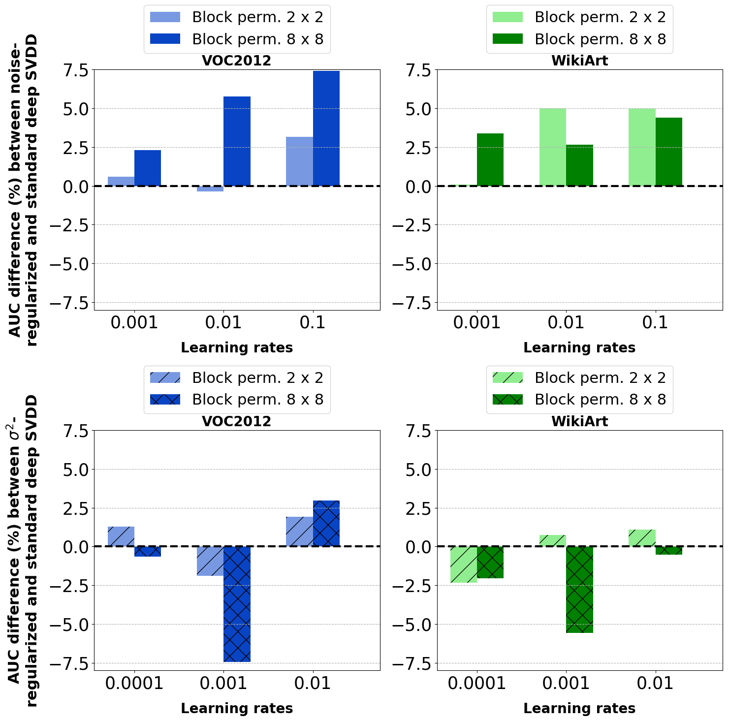
Figure 1: A positive performance difference indicates that the proposed variant outperforms the standard deep SVDD model. Models are trained with the soft-boundary objective function. For the top row, the learning rates are those of the linear layer $g(\cdot\ ;\mathcal{W}_{1})$, for all other layers it is lower by a factor of 10. The learning rates in the bottom row are used in all layers of the network.

Table II compares the performance of models on the block permutation test sets which contain normal samples and anomalies generated with method 1 (refer Section V-A). On the block permutation test sets, the GEO model [22] significantly outperforms all the other methods. The same can also be observed for the one-vs-all setup in Table III. The anomalies in the block permutation test set and the normal samples (from a single class) in the one-vs-all setup contain specific geometrical structures that are highly distinguishable from their counterparts. Therefore, the GEO model trained to distinguish salient geometrical features of transformed images performs well on these samples due to the presence of significant geometrical structures. However, the GEO model does not perform well given anomalies that do not portray any apparent geometrical structure such as the strokes anomalies created using method 2 in Section V-A. We elaborate on this later with reference to Table III and IV. In Table II, we also note that at least one of the proposed regularized variants of deep SVDD (mostly the noise-regularized variant, i.e. D. SVDD w/ bias & noise reg.) has the second best performance after the GEO method for a majority of the block permutation settings. In Table III, the OC-SVM model with CNN features performs second best on the one-vs-all setup. Additionally, we observe that the noise-regularized model appears to be more effective than the variance-regularized model in a majority of the cases. For some experiments, we also observe that the shallow models with features from PCA yield better performance than features from ResNet-18, which is partially due to the pooling operation in the pretrained model that has removed some useful features of the anomalies. This will be shown in Figure 2 and discussed later. We also note that the performance achieved by the different models for the one-vs-all setup on CIFAR10 in Table III is similar to other works [13, 22].

The GEO method does not perform well on the strokes test sets as shown in Table III and IV. Since there is no apparent geometrical structure in the strokes test sets due to the various shapes and lengths of the strokes, the GEO model can not take advantage of the geometrical structure of the anomalies and does not perform well in this setting. This suggests that the use of the GEO model may not be appropriate for other types of anomalies that do not portray any apparent geometrical structure. For the shallow models and all variants of deep SVDD, their detections do not directly rely on the presence of geometrical structure in the anomalies and hence, can be used generically for anomaly detection regardless of the types of anomalies. Based on Table III and IV, the variance-regularized model performs better than the other models on the VOC2012 dataset for a majority of the settings, while the noise-regularized model is more effective on the CIFAR10 and WikiArt dataset. It can also be observed that the deep SVDD model and its variants perform better on easier settings, i.e. samples with larger distortion of the natural image.

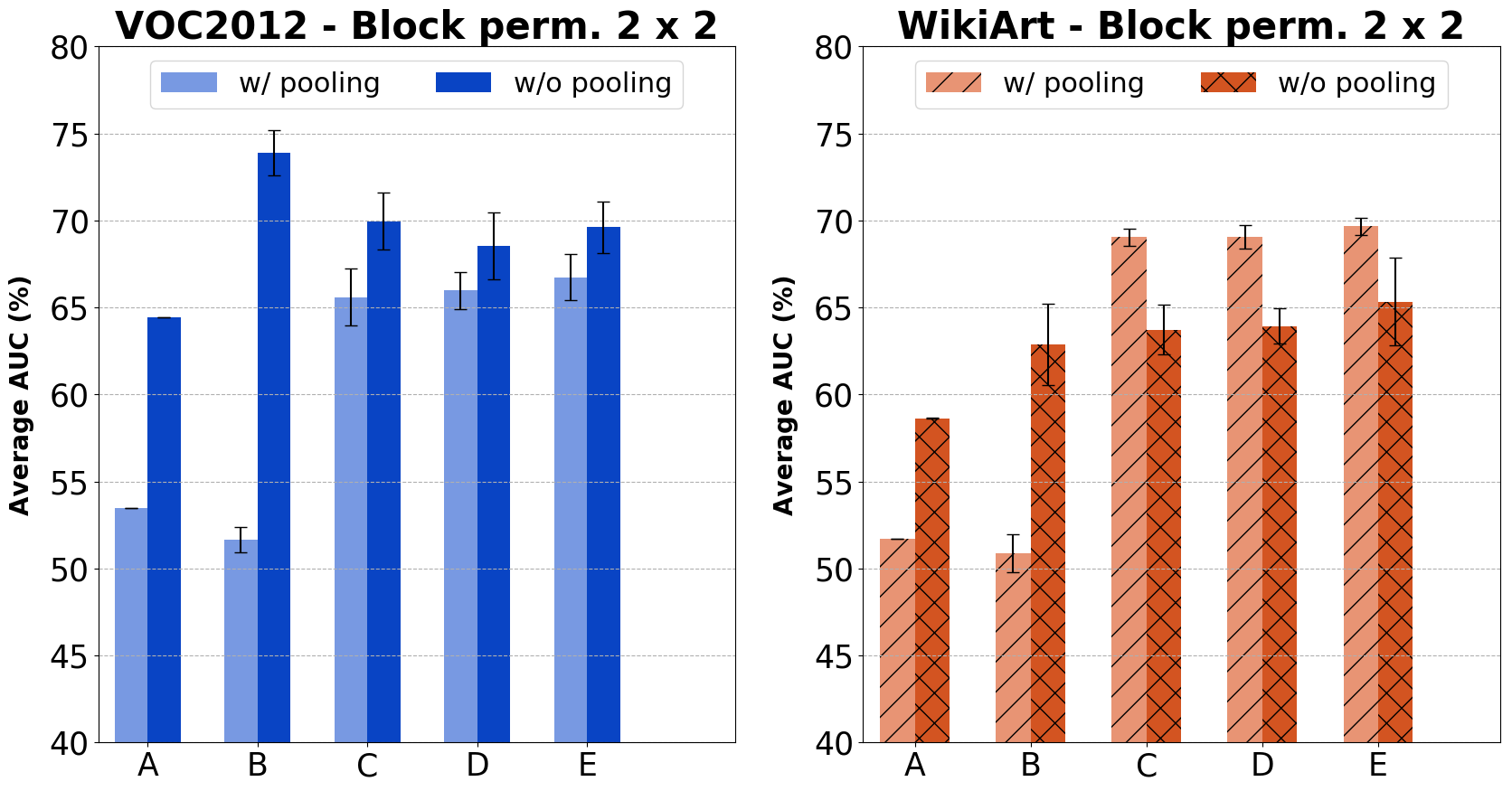
Figure 2: Performance of models with and without the pooling layer in ResNet-18. The deep SVDD model and its variants are trained with the one-class objective function. We denote the OC-SVM, IF, standard deep SVDD [13], deep SVDD with bias term, and noise-regularized deep SVDD models as A, B, C, D, and E, respectively.

Regarding impact of learning rates, we observe that both regularized and non-regularized deep SVDD models generally perform better at low learning rate ($0.001$) as compared to high learning rates ($0.01$ and $0.1$). Close examinations on the experiments also reveal that both regularized variants and the standard deep SVDD model [13] collapse to a single point $\phi\equiv c$ at high learning rates ($0.01$ and $0.1$). For the variance-regularized method, we observe in our preliminary experiments that fixing the variance threshold $d_{\tilde{t}}$ to a sufficiently small constant can effectively prevent mode collapse for high learning rates, but such a stringent threshold can severely hinder feature learning. Thus, we choose to adopt the annealing approach to gradually decrease the variance threshold $d_{\tilde{t}}$ instead. All results reported at high learning rates ($0.01$ and $0.1$) in Figure 1 and Table V, are the test performances of the best performing model before the hypersphere collapses. Although both regularized models and the standard deep SVDD collapse under high learning rates, D. SVDD w/ bias & noise reg. model achieves better performance convergence than the D. SVDD model for a majority of the experiments as shown in Table V. Moreover, even though the D. SVDD w/ bias & $\sigma^{2}$ reg. model is less effective than the D. SVDD w/ bias & noise reg. model, it shows better performance convergence than the D. SVDD model for half of the experiments at high learning rates ($0.01$ and $0.1$). These observations suggest that the regularizers may have curbed the impact of mode collapse to an extent. Figure 1 clearly depicts the trend of the performance difference between the proposed methods and the standard deep SVDD across different learning rates. For the noise-regularized variant of deep SVDD, we observe in general a higher performance gain over the standard deep SVDD model as the learning rate increases. Meanwhile, no obvious trend is shown for the performance difference between the variance-regularized model and the standard deep SVDD model. For all other experiments, we choose the low learning rate of $10^{-3}$ due to better performance and stability against mode collapse.

In addition, we remove the pooling layer of ResNet-18 and compare the performance of the models with the results from Table II. In Figure 2, the OC-SVM and IF models generally show better performance when given ResNet-18 features without pooling. For some settings, these shallow models even outperform their counterparts with PCA features (refer Table II). The improvement in performance suggests that the pooling operation may have removed certain useful features for the anomalous samples. Without the pooling layer, the deep SVDD model and its variants consistently perform better on the VOC2012 dataset and worse for the WikiArt dataset.

TABLE VI: Performance of the semi-supervised deep SVDD model and its variants in one-class mode. Performance for one-vs-all setup is the average of $10$ normal classes. For each normal class, only a single anomaly class (out of nine) was included during training and each anomaly class setting was ran five times, resulting in a total of $9\times 5$ runs.

	CIFAR10	VOC2012			WikiArt
Models	One -vs- all	$\Diamond$Bp.$8$ $\Box$St.$9$ $\bigtriangleup$St.$5$	$\Diamond$St.$9$ $\Box$Bp.$8$ $\bigtriangleup$Bp.$2$	$\Diamond$St.$9$ $\Box$St.$5$ $\bigtriangleup$Bp.$2$	$\Diamond$Bp.$8$ $\Box$St.$9$ $\bigtriangleup$St.$5$	$\Diamond$St.$9$ $\Box$Bp.$8$ $\bigtriangleup$Bp.$2$	$\Diamond$St.$9$ $\Box$St.$5$ $\bigtriangleup$Bp.$2$
D. SVDD [14]	$80.9$$\pm$$6$	$94.297\,914\,095\,272\,97$$\pm$$2$	$87.406\,764\,691\,716\,18$$\pm$$5$	$86.658\,047\,207\,593\,4$$\pm$$3$	$93.888\,288\,247\,528\,21$$\pm$$3$	$85.941\,608\,497\,895\,46$$\pm$$6$	$82.820\,419\,041\,371\,1$$\pm$$2$
D. SVDD w/ bias	$80.8$$\pm$$6$	$94.122\,855\,633\,780\,88$$\pm$$2$	$85.378\,585\,056\,597\,13$$\pm$$5$	$82.177\,940\,825\,207\,2$$\pm$$3$	$94.585\,803\,379\,420\,63$$\pm$$2$	$85.429\,179\,632\,988\,87$$\pm$$5$	$87.625\,398\,674\,642\,7$$\pm$$5$
D. SVDD w/ bias & noise reg.	$81.2$$\pm$$6$	$96.345\,544\,852\,587\,27$$\pm$$1$	$87.866\,016\,286\,321\,57$$\pm$$4$	$87.943\,484\,111\,613$$\pm$$3$	$93.241\,029\,802\,864\,77$$\pm$$1$	$90.757\,912\,625\,957\,72$$\pm$$4$	$85.434\,849\,798\,029\,3$$\pm$$5$
D. SVDD w/ bias & $\sigma^{2}$ reg.	$80.0$$\pm$$6$	$89.389\,538\,988\,908\,62$$\pm$$4$	$81.114\,929\,543\,130\,44$$\pm$$6$	$83.576\,581\,851\,495\,19$$\pm$$4$	$91.917\,004\,415\,501\,04$$\pm$$4$	$87.817\,091\,085\,438\,45$$\pm$$4$	$88.606\,941\,229\,864\,8$$\pm$$4$
Bp. = Block perm.  St. = Strokes ;  $\Diamond$train set  $\Box$val. set  $\bigtriangleup$test set

Lastly, we also show in Table VI, the performance of the deep SVDD model and its variants with semi-supervised learning. For the regularized variants, we apply regularization to all labeled and unlabeled samples in a similar manner as the unsupervised regularized variants. For the one-vs-all setup conducted with the CIFAR10 dataset, the D. SVDD w/ bias & noise reg. model has the best performance. For the image alteration anomalies setup conducted only with the VOC2012 and WikiArt datasets, we ensure that the models are not trained and tested with the same type of anomalies to study the generalization capability of the models to a different type of anomaly. In the first two columns for VOC2012 and WikiArt datasets, the models were trained and validated/tested with different type of anomalies (block permutation vs. strokes). It can be seen that the models trained with block permutation train set show better performance on strokes test set, as compared to models trained with strokes train set and tested on block permutation test sets. Similar to unsupervised learning, the semi-supervised noise-regularized variant generally achieves better performance than the variance-regularized variant. For almost all settings, it can be observed that the proposed regularizers (mostly D. SVDD w/ bias & noise reg.) perform notably better than the other deep SVDD models.

VII Conclusion

In this work, we considered two simple and effective regularization methods against mode collapse in deep SVDD. Even though the minibatch variance regularization method provided more control over the amount of regularization applied, the regularization method based on random noise injection generally performed better. Additionally, we demonstrated that both regularization methods performed better than the state-of-the-art GEO method on the strokes test sets that do not portray apparent geometrical structures. We also showed that either one of the regularized variants achieved better performance than the standard deep SVDD and other classification-based models in a majority of the experiments. Moreover, we learned that the standard deep SVDD model and its variants performed better and were more stable at low learning rate. As noted by one of the reviewers, our proposed regularizers could be of interest for mitigating the mode collapse problem in GANs.

References

[1]
V. Chandola, A. Banerjee, and V. Kumar, “Anomaly detection: A survey,”
ACM computing surveys (CSUR), vol. 41, no. 3, p. 15, 2009.
[2]
M. Ramadas, S. Ostermann, and B. Tjaden, “Detecting anomalous network traffic
with self-organizing maps,” in International Workshop on Recent
Advances in Intrusion Detection. Springer, 2003, pp. 36–54.
[3]
S. Zhai, Y. Cheng, W. Lu, and Z. Zhang, “Deep structured energy based models
for anomaly detection,” arXiv preprint arXiv:1605.07717, 2016.
[4]
N. Shone, T. Ngoc, V. Phai, and Q. Shi, “A deep learning approach to network
intrusion detection,” IEEE Transactions on Emerging Topics in
Computational Intelligence, vol. 2, no. 1, pp. 41–50, 2018.
[5]
D. Huang, D. Mu, L. Yang, and X. Cai, “Codetect: financial fraud detection
with anomaly feature detection,” IEEE Access, vol. 6, pp.
19 161–19 174, 2018.
[6]
J. Goh, S. Adepu, M. Tan, and Z. Lee, “Anomaly detection in cyber physical
systems using recurrent neural networks,” in 2017 IEEE 18th
International Symposium on High Assurance Systems Engineering (HASE). IEEE, 2017, pp. 140–145.
[7]
I. Steinwart, D. Hush, and C. Scovel, “A classification framework for anomaly
detection,” Journal of Machine Learning Research, vol. 6, no. Feb,
pp. 211–232, 2005.
[8]
C. Zhou and R. Paffenroth, “Anomaly detection with robust deep autoencoders,”
in Proceedings of the 23rd ACM SIGKDD International Conference on
Knowledge Discovery and Data Mining, ser. KDD ’17. New York, NY, USA: ACM, 2017, pp. 665–674. [Online].
Available: http://doi.acm.org/10.1145/3097983.3098052
[9]
T. Schlegl, P. Seeböck, S. Waldstein, U. Schmidt-Erfurth, and G. Langs,
“Unsupervised anomaly detection with generative adversarial networks to
guide marker discovery,” in International Conference on Information
Processing in Medical Imaging. Springer, 2017, pp. 146–157.
[10]
B. Schölkopf, R. Williamson, A. Smola, J. Shawe-Taylor, and J. Platt,
“Support vector method for novelty detection,” in Advances in neural
information processing systems, 2000, pp. 582–588.
[11]
D. Tax and R. Duin, “Support vector data description,” Machine
learning, vol. 54, no. 1, pp. 45–66, 2004.
[12]
F. Liu, K. Ting, and Z. Zhou, “Isolation forest,” in 2008 Eighth IEEE
International Conference on Data Mining. IEEE, 2008, pp. 413–422.
[13]
L. Ruff, R. Vandermeulen, N. Goernitz, L. Deecke, S. Siddiqui, A. Binder,
E. Müller, and M. Kloft, “Deep one-class classification,” in
International Conference on Machine Learning, 2018, pp. 4393–4402.
[14]
L. Ruff, R. Vandermeulen, N. Görnitz, A. Binder, E. Müller,
K. Müller, and M. Kloft, “Deep semi-supervised anomaly detection,”
arXiv preprint arXiv:1906.02694, 2019.
[15]
M. Arjovsky and L. Bottou, “Towards principled methods for training generative
adversarial networks,” in 5th International Conference on Learning
Representations, ICLR 2017, Toulon, France, April 24-26, 2017, Conference
Track Proceedings, 2017. [Online]. Available:
https://openreview.net/forum?id=Hk4_qw5xe
[16]
T. Salimans, I. Goodfellow, W. Zaremba, V. Cheung, A. Radford, and X. Chen,
“Improved techniques for training gans,” in Advances in neural
information processing systems, 2016, pp. 2234–2242.
[17]
E. Candès, X. Li, Y. Ma, and J. Wright, “Robust principal component
analysis?” Journal of the ACM (JACM), vol. 58, no. 3, p. 11, 2011.
[18]
L. Beggel, M. Pfeiffer, and B. Bischl, “Robust anomaly detection in images
using adversarial autoencoders,” arXiv preprint arXiv:1901.06355,
2019.
[19]
L. Deecke, R. Vandermeulen, L. Ruff, S. Mandt, and M. Kloft, “Image anomaly
detection with generative adversarial networks,” in Joint European
Conference on Machine Learning and Knowledge Discovery in Databases. Springer, 2018, pp. 3–17.
[20]
H. Zenati, C. Foo, B. Lecouat, G. Manek, and V. Chandrasekhar, “Efficient
gan-based anomaly detection,” arXiv preprint arXiv:1802.06222, 2018.
[21]
S. Akcay, A. Atapour-Abarghouei, and T. Breckon, “Ganomaly: Semi-supervised
anomaly detection via adversarial training,” in Asian Conference on
Computer Vision. Springer, 2018, pp.
622–637.
[22]
I. Golan and R. El-Yaniv, “Deep anomaly detection using geometric
transformations,” in Advances in Neural Information Processing
Systems, 2018, pp. 9758–9769.
[23]
T. Che, Y. Li, A. Jacob, Y. Bengio, and W. Li, “Mode regularized generative
adversarial networks,” arXiv preprint arXiv:1612.02136, 2016.
[24]
A. Srivastava, L. Valkov, C. Russell, M. Gutmann, and C. Sutton, “Veegan:
Reducing mode collapse in gans using implicit variational learning,” in
Advances in Neural Information Processing Systems, 2017, pp.
3308–3318.
[25]
C. Chang, C. Hubert Lin, C. Lee, D. Juan, W. Wei, and H. Chen, “Escaping from
collapsing modes in a constrained space,” in Proceedings of the
European Conference on Computer Vision (ECCV), 2018, pp. 204–219.
[26]
D. Berthelot, T. Schumm, and L. Metz, “Began: Boundary equilibrium generative
adversarial networks,” arXiv preprint arXiv:1703.10717, 2017.
[27]
B. Chen, W. Deng, and J. Du, “Noisy softmax: Improving the generalization
ability of dcnn via postponing the early softmax saturation,” in
Proceedings of the IEEE Conference on Computer Vision and Pattern
Recognition, 2017, pp. 5372–5381.
[28]
L. Xie, J. Wang, Z. Wei, M. Wang, and Q. Tian, “Disturblabel: Regularizing cnn
on the loss layer,” in Proceedings of the IEEE Conference on Computer
Vision and Pattern Recognition, 2016, pp. 4753–4762.
[29]
L. Rosasco, E. Vito, A. Caponnetto, M. Piana, and A. Verri, “Are loss
functions all the same?” Neural Computation, vol. 16, no. 5, pp.
1063–1076, 2004.
[30]
A. Krizhevsky, G. Hinton et al., “Learning multiple layers of features
from tiny images,” Citeseer, Tech. Rep., 2009.
[31]
M. Everingham, L. Van Gool, C. Williams, J. Winn, and A. Zisserman, “The
PASCAL Visual Object Classes Challenge 2012 (VOC2012)
Results,”
http://www.pascal-network.org/challenges/VOC/voc2012/workshop/index.html.
[32]
“Wikiart.org - visual art encyclopedia,” https://www.wikiart.org/, (Accessed
on 05/24/2019).
[33]
W. Tan, C. Chan, H. Aguirre, and K. Tanaka, “Artgan: Artwork synthesis with
conditional categorical gans,” in 2017 IEEE International Conference
on Image Processing (ICIP). IEEE,
2017, pp. 3760–3764.
[34]
W. Xu, D. Evans, and Y. Qi, “Feature squeezing: Detecting adversarial examples
in deep neural networks,” arXiv preprint arXiv:1704.01155, 2017.
[35]
D. Canali, M. Cova, G. Vigna, and C. Kruegel, “Prophiler: a fast filter for
the large-scale detection of malicious web pages,” in Proceedings of
the 20th international conference on World wide web. ACM, 2011, pp. 197–206.
[36]
K. He, X. Zhang, S. Ren, and J. Sun, “Deep residual learning for image
recognition,” in Proceedings of the IEEE conference on computer vision
and pattern recognition, 2016, pp. 770–778.
[37]
D. Kingma and J. Ba, “Adam: A method for stochastic optimization,”
arXiv preprint arXiv:1412.6980, 2014.
[38]
A. Paszke, S. Gross, S. Chintala, G. Chanan, E. Yang, Z. DeVito, Z. Lin,
A. Desmaison, L. Antiga, and A. Lerer, “Automatic differentiation in
pytorch,” 2017.
[39]
S. Zagoruyko and N. Komodakis, “Wide residual networks,” arXiv preprint
arXiv:1605.07146, 2016.
[40]
F. Chollet et al., “Keras,” https://github.com/fchollet/keras, 2015.
[41]
S. Erfani, S. Rajasegarar, S. Karunasekera, and C. Leckie, “High-dimensional
and large-scale anomaly detection using a linear one-class svm with deep
learning,” Pattern Recognition, vol. 58, pp. 121–134, 2016.