Rough basin boundaries in high dimension: Can we classify them experimentally?

Abstract

We show that a known condition for having rough basin boundaries in bistable 2D maps holds for high-dimensional bistable systems that possess a unique nonattracting chaotic set embedded in their basin boundaries. The condition for roughness is that the cross-boundary Lyapunov exponent $\lambda_{x}$ on the nonattracting set is not the maximal one. Furthermore, we provide a formula for the generally noninteger co-dimension of the rough basin boundary, which can be viewed as a generalization of the Kantz-Grassberger formula. This co-dimension that can be at most unity can be thought of as a partial co-dimension, and, so, it can be matched with a Lyapunov exponent. We show in 2D noninvertible- and 3D invertible minimal models, that, formally, it cannot be matched with $\lambda_{x}$. Rather, the partial dimension $D_{0}^{(x)}$ that $\lambda_{x}$ is associated with in the case of rough boundaries is trivially unity. Further results hint that the latter holds also in higher dimensions. This is a peculiar feature of rough fractals. Yet, $D_{0}^{(x)}$ cannot be measured via the uncertainty exponent along a line that traverses the boundary. Indeed, one cannot determine whether the boundary is a rough or a filamentary fractal by measuring fractal dimensions. Instead, one needs to measure both the maximal and cross-boundary Lyapunov exponents numerically or experimentally.

1 Introduction

Beside chaotic attractors, nonattracting chaotic sets also have practical relevance [1]. They are associated with e.g. basins of attraction in multistabe systems, or, long-lived chaotic transients. Respective global properties quantified by characteristic numbers determine predictability and the life time of trajectories within a vicinity of the nonattracting set. Regarding nonattracting sets the most relevant concept of predictability is that of the second kind, concerning the outcome of an experiment in terms of the final state of the system out of a few alternatives [2]. This kind of predictability can be quantified by the uncertainty exponent [3, 4], expressing the improvement of predictability of the outcome by determining the initial condition more precisely. To put this in to context, we note that attractors, on the other hand, are associated with predictability of the first kind only, when we are concerned with how the error in the prediction of the future state of the system changes as we change the precision in the definition of the initial conditions. Error growth or decline in specific directions [5] is measured by a spectrum of Lyapunov exponents (LE); and, concerning an initial condition with small random error, it is the maximal positive LE (MLE) that determines the asymptotic but infinitesimal error growth for trajectories confined to the invariant set that supports a measure. Lyapunov exponents are thus regarded to quantify local instabilities, while the escape rate $\kappa$, the inverse of the expected or characteristic life time of trajectories mentioned above, is regarded to quantify global instability. LEs can be defined for both attractors and nonattracting invariant sets that support a measure, while attractors are clearly globally stable with no escape from them. [1]

Global characteristic numbers are in fact not completely independent. First, the uncertainty exponent $\alpha$ has a straightforward one-to-one connection with the fractal dimension $D_{b,0}$ of the basin boundary, being simply the co-dimension $\alpha=D-D_{b,0}$, where $D$ is the dimension of the phase space, implying that the more space-filling the set, the poorer the predictability of the second kind. Second, a connection (i) of the predictability of the second kind and global instability, and, third, another connection (ii) of the global and local instabilities, can be given as follows. We consider here discrete-time bistable systems that are possibly composed of coupling two subsystems (both of which can be multi-dimensional):

$$X_{i+1} = f_{X}(X_{i},Y_{i};\epsilon_{X},p),$$ (1)

$$Y_{i+1} = f_{Y}(X_{i},Y_{i};\epsilon_{Y}),$$ (2)

where the subsystems decouple for $\epsilon_{X}=\epsilon_{Y}=0$, such that $f_{X}(X,Y;\epsilon_{X}=0)=\tilde{f}_{X}(X)$ and $f_{Y}(X,Y;\epsilon_{Y}=0)=\tilde{f}_{Y}(Y)$. We assume that the unperturbed ($\epsilon_{X}=0$) subsystem (1) has two co-existing attractors, while the unperturbed ($\epsilon_{Y}=0$) subsystem (2) has a unique globally attracting set. That is, the bistability of the coupled system derives from that of (1). Furthermore, we assume that a single nonattracting chaotic set is embedded in the basin boundary of either (1) ($\epsilon_{X}=0$) or the coupled system (1)-(2), and so they possesses a single unstable dimension in which escape can occur. Such a nonattracting set (either a chaotic saddle or repeller) is said to be low-dimensional [1]. That is, the dimensionality of the nonattracting set in this sense is not to be confused with the dimensionality of the phase space of the system. Note that the stable manifold of the unique nonattracting set coincides with the basin boundary. For low-dimensional nonattracting chaotic sets embedded in so-called filamentary fractal boundaries, “locally consisting of a Cantor set of smooth curves or surfaces” [1], the Kantz-Grassberger relation [6] holds:

$$\kappa=\lambda_{x}(1-D_{1}^{(x)}),$$ (KG)

where $\lambda_{x}$ and $D_{1}^{(x)}$ are the cross-boundary LE (i.e. the Lyapunov exponent describing the instability of the motion across the smooth boundary filament) and associated [1] partial information dimension, respectively. It implies that

(i)

upon a change that leaves the LEs (and so the predictability of the first kind) practically unchanged, a longer characteristic life time, i.e. a greater global stability, is implied by a poorer predictability of the second kind [2], and vice-versa; and

(ii)

the global instability quantified by $\kappa$ is in general weaker than the local instability quantified by $\lambda_{x}$, simply because $0\leqq D_{1}^{(x)}\leqq 1$, as though the intricate folded geometry could trap the trajectory.

As for (i) above the change may be (i.a) wrt. a parameter $p$, while $\epsilon_{X}=0$ in eq. (1), or, (i.b) by introducing a perturbation, $\epsilon_{X}\neq 0$. In the latter case it is meant that the basin boundary of the coupled system is still filamentary, and that the LEs of the uncoupled and coupled system are approximately the same. In the case of such a weak coupling, we use the term “perturbation” for $Y$ from the point of view of $X$. As shown by Wouters and Lucarini [7, 8], switching on the coupling between the subsystems by setting $\epsilon_{X}\neq 0$ and/or $\epsilon_{Y}\neq 0$ can be formally treated as a perturbation using Ruelle’s [9] response theory.

As discussed in Sec. 2.2 in the following, for another type of boundary, a continuous fractal boundary, which is rough, nowhere differentiable, KG does not apply, but rather a more generic formula (24), in which $\lambda_{x}$ and $(1-D_{1}^{(x)})$ are replaced by the MLE $\lambda_{max}$ and the co-dimension of the boundary, i.e. $\alpha$, respectively. This implies completely new properties, including the generic invalidity of (i) and (ii), which will be further discussed in Sec. 5. It becomes thus possible to have a very poor predictability of the second kind due to a strongly space-filling boundary, while the trajectory life time is fairly short, with a global instability being about the same as the local cross-boundary instability. The obvious – and perhaps very common – way that this situation can arise is that we have a bistable system ($X$) that is perturbed by another system ($Y$) whose behaviour is noise-like  compared to that of the bistable one. A weak enough noise-like perturbation does not alter the global instability [10] but renders the outcome completely unpredictable (although the thickness of the boundary scales with the perturbation strength). That is, the poor predictability of the first kind of the fast system $Y$ will impact the predictability of the second kind of the coupled system. In the extreme, predictability of the second kind is completely lost, $\alpha=0$, with an extreme time-scale separation $\lambda_{x}/\lambda_{max}\rightarrow 0$, even if in the uncoupled/unperturbed ($\epsilon_{X}=0$) bistable system $X$ we had perfect predictability of the second kind, $D_{1}^{(x)}=0$, $\alpha=1$.

We encountered such a situations in the case of a bistable climate model of intermediate complexity [11]. In this model the so-called snowball-snow free bistability is created by the ice-albedo positive feedback. This effect can be modeled by very simple 0-D energy balace models (EBM) (where “0” in “0-D” refers to the spatial extension of variables). In our model studied in [11] a 1-D diffusive heat equation serves the same purpose, which, however, has in common with the 0-D EBM a nonchaotic solution. When this ocean-ice model component ($X$) was coupled with the chaotic atmosphere ($Y$), the originally regular basin boundary was found to turn into a practically space-filling object.

Attaining our motivating objective, we are able to claim here that what we encountered was in fact a rough continuous very thick fractal, because, first, the condition $\lambda_{x}<\lambda_{max}$ found for 2D maps [12, 13] we argue in Sec. 2.1 to be applicable to high-dimensional systems, and, second, the condition was in fact satisfied by the coupled climate model. As for the second point, we did not measure the cross-boundary LE of the coupled/perturbed climate model, only the MLE, but we did measure $\lambda_{x}$ of the 1-D EBM in [14], and clearly it is not altered significantly by a rather weak coupling and the weakened diffusivity applied in [11], while $\lambda_{x}$ and $\lambda_{max}$ are obviously vastly different representing climatic and weather processes, respectively.

Next, in Sec. 2 we reproduce the condition for roughness in a general setting, and also provide dimension formulae for rough boundaries. In Sec. 3 we provide minimal models that feature rough boundaries, among them a prototypical model for a new kind of mixed filamentary-rough boundary. In Sec. 4 we report on our numerical computations performed to determine the fractal dimension of the boundary. Finally, in Sec. 5 we discuss our results here and those in [11], and pose some open questions of geophysical relevance.

2 Theory

2.1 Condition for roughness

Grebogi et al. [12] provided for the first time a condition for the roughness of the basin boundary in a 2D map when this rough boundary can be described as a Weierstarss function in terms of a Fourier series whose derivative is a nonconvergent series. The latter can be viewed as a recipe for creating a map with a rough basin boundary. However, Vollmer et al. [13] derives the same condition in an alternative way, not requiring the boundary to be described by a Weierstrass function. This is what we reproduce next, pointing out in addition that 1) it applies not only to 2D maps but to any high-dimensional one, and 2) also to systems with a fractal boundary which is filamentary when $\lambda_{x}=\lambda_{max}$.

Assume that $x$ and $y$ denote some local coordinates that describe motions in a coarse sense “across” and “along” a basin boundary, respectively, of a discrete-time dynamical system. Therefore, the small perturbations around the boundary evolve as:

$$\delta x_{n} = \prod_{i=1}^{n}\Lambda_{x,i}\delta x_{0}+\epsilon\sum_{j=0}^{n-1}\prod_{i=1}^{j}\Lambda_{x,i}\delta y_{n-1-j},$$ (3)

$$\delta y_{n} = \prod_{i=1}^{n}\Lambda_{y,i}\delta y_{0},$$ (4)

where the $\Lambda$’s are local Lyapunov numbers. Note that eq. (3) derives from the linear evolution equation (being a recursive formula)

$$\delta x_{i+1}=\Lambda_{x,i}\delta x_{i}+\epsilon\delta y_{i};$$ (5)

and from eq. (4) the $x$-dynamics is readily transformed out, having utilized the fact that the dynamics is constrained to a surface being the basin boundary. Note also that a time-independent constant $\epsilon$ means that, to start with, we consider the case of additive perturbation, i.e., $f_{x}(x,y;\epsilon_{X}=\epsilon)=\tilde{f}_{x}(x)+\epsilon y$ in eq. (1) simplified to a 2D situation. In eq. (3) we express $\delta y_{n-1-j}$ using eq. (4) and rearrange it as:

$$\frac{\delta x_{0}}{\delta y_{0}}=-\epsilon\frac{\sum_{j=0}^{n-1}\prod_{i=1}^{j}\Lambda_{x,i}\prod_{i=1}^{n-1-j}\Lambda_{y,i}}{\prod_{i=1}^{n}\Lambda_{x,i}},$$ (6)

which owes to the fact that $\delta x_{n}$ is bounded when the perturbation is chosen in a special way that the perturbed trajectory stays on the boundary. That is, the degree-of-freedom of choosing such a perturbation is one, not two. With constant local Lyapunov numbers this equation would simplify to:

$$\frac{\delta x_{0}}{\delta y_{0}}=-\epsilon\frac{\sum_{j=0}^{n-1}\Lambda_{x}^{j}\Lambda_{y}^{n-1-j}}{\Lambda_{x}^{n}}=-\frac{\epsilon}{\Lambda_{x}}\sum_{j=0}^{n-1}\left(\frac{\Lambda_{y}}{\Lambda_{x}}\right)^{n-1-j}=-\frac{\epsilon}{\Lambda_{x}}\sum_{i=0}^{n-1}r^{i},$$ (7)

$$r=\frac{\Lambda_{y}}{\Lambda_{x}}.$$ (8)

A finite value for the left hand side would mean in the limit of $n\rightarrow\infty$ that the boundary is locally smooth. It turns out that it is only possible if the Lyapunov number or exponent is smaller across the boundary than the other one ($r<1$), yielding a convergent series. If not ($r>1$), the boundary is not smooth locally but can be viewed as rough, not differentiable. When $\Lambda_{x,i}$, $\Lambda_{y,i}$ do vary over the nonattracting set, and so in time along a trajectory, in terms of $j$ appearing in eq. (6), these are the smaller values of $j$ that need to be kept in check, corresponding to larger powers of some $r$ of the time-independent formula (7), and so in the limit, these are indeed the average Lyapunov exponents, as arithmetic averages of $\ln\Lambda_{x,y,i}$’s, that determine whether the series is convergent. That is,

$$\lim_{n\to\infty}\frac{1}{\sum_{j=0}^{n-1}\left(\frac{\Lambda_{y}}{\Lambda_{x}}\right)^{n-1-j}}=0\Rightarrow$$ (9)

$$\lim_{n\to\infty}\frac{1}{\sum_{j=0}^{n-1}\frac{\prod_{i=1}^{n-1-j}\Lambda_{y,i}}{\prod_{i=1}^{n-1-j}\Lambda_{x,i}}}=0\Rightarrow$$ (10)

$$\lim_{n\to\infty}\frac{\prod_{i=1}^{n}\Lambda_{x,i}}{\sum_{j=0}^{n-1}\prod_{i=1}^{j}\Lambda_{x,i}\prod_{i=1}^{n-1-j}\Lambda_{y,i}}=0.$$ (11)

(We can denote the (geometric) average Lyapunov numbers simply by $\Lambda_{x}$, $\Lambda_{y}$, just like the constant local Lyapunov numbers in the special case.) Besides that, we note that a spatial dependence of $\delta x_{0}/\delta y_{0}$ arises from the finite terms of the series. We also point out that when the coupling is also nonlinear, such that the generic form of eq. (1) applies, which results in a time-dependent $\epsilon_{i}$ (to replace the constant in eq. (5)), the condition on roughness is unchanged. Next, we point out two more possible generalisations.

1) Consider a multi-dimensional boundary, with state variables $y_{d}$ “along” this hyper-surface, $d=1,\dots,D-1$, $D$ being the phase space dimension. Then, eqs. (3) and (4) generalise straightforwardly as:

$$\delta x_{n} = \prod_{i=1}^{n}\Lambda_{x,i}\delta x_{0}+\sum_{d=1}^{D-1}\epsilon_{d}\sum_{j=0}^{n-1}\prod_{i=1}^{j}\Lambda_{x,i}\delta y_{d,n-1-j},$$ (12)

$$\delta y_{d,n} \sim \Lambda_{y}^{n},$$ (13)

where we retain the simplified notation $\Lambda_{y}$ for the maximal one out of all $\Lambda_{y,d}$. Note that in eq. (13) we only state the asymptotic behaviour, indicated by the symbol $\sim$, which also means that we suppress the indication of a constant of proportionality. We also point out that it is the maximal $\Lambda_{y}$ indeed that appears in all $D-1$ components of the subsystem (13); the components differ only wrt. the suppressed constant of proportionality. Therefore, we can express a directional derivative by rearranging (12) for $\delta x_{0}$ and dividing it by a normalised linear combination $\sum_{d}^{D-1}c_{d}\delta y_{d,0}$, where $\sum_{d}^{D-1}c_{d}=1$. This will be finite again, clearly, if $r<1$. It should be noted that eqs. (13) apply generically, i.e., with probability one, unless a direction is taken for the directional derivative that aligns with a covariant Lyapunov vector (CLV) of the system [5]. In that case eqs. (13) modify to be

$$\delta y_{d,n}\sim\Lambda_{y,d^{*}}^{n},$$ (14)

where $\Lambda_{y,d^{*}}$ can be any one of the positive $\Lambda_{y,d}$’s, belonging to the CLV in question, the same value applying to all components of (14). In this case it is possible that the derivative exists given that $\Lambda_{y,d^{*}}/\Lambda_{x}<1$ while we have a rough surface because $r>1$, i.e., the surface is not necessarily rough in every direction.

2) Roughness can be regarded as a local property because the derivative belongs to a particular locale on the boundary. The neighbourhood of such a locale can be characterized the same way in the case of a filamentary fractal boundary and a regular boundary. On the other hand, roughness should be considered as a global property too because if the derivative does not exists in one locale, neither does it exist in any other one, given that the condition is based on global properties, the average Lyapunov numbers/exponents. Therefore, also a filamentary fractal boundary should turn rough upon some change that changes $\lambda_{x}=\lambda_{max}$ to $\lambda_{x}<\lambda_{max}$. This change may be brought about either by changing $p$ of the coupled system (1)-(2) from some $p_{1}$ to $p_{2}$, or, by switching on the coupling going from $\epsilon_{X}=0$ to $\epsilon_{X}\neq 0$. However, the result is a new type of rough boundary.

2.2 Dimension formulae

2.2.1 Co-dimension of the basin boundary

In order to establish dimension formulae applying to rough boundaries, we invoke the following generic relations established in [15]. The information dimensions of the unstable and stable manifolds of a nonattracting invariant set, respectively, are:

$$D_{u,1}=U+I+\frac{K_{1}-\sum_{i=1}^{I}\lambda_{i}^{-}}{\lambda_{I+1}^{-}},$$ (15)

$$D_{s,1}=S+J+\frac{K_{1}-\sum_{j=1}^{J}\lambda_{j}^{+}}{\lambda_{J+1}^{-}},$$ (16)

where $U$ ($S$) is the number of positive $\lambda_{i}^{+}$ (negative $\lambda_{i}^{-}$) Lyapunov exponents ($U+S=D$, $-\lambda_{S}^{-}\leq-\lambda_{S-1}^{-}\leq\dots\leq-\lambda_{1}^{-}\leq 0\leq\lambda_{1}^{+}\leq\dots\leq\lambda_{U-1}^{+}\leq\lambda_{U}^{+}$), $I$ ($J$) is the largest integer for which the numerator of the fraction in eq. (15) ((16)) is still positive, and

$$K_{1}=\sum_{j=1}^{U}\lambda_{j}^{+}D_{1}^{(j)}$$ (17)

is the so-called metric entropy. In the latter $D_{1}^{(j)}$ are the partial dimensions belonging to the LEs $\lambda_{j}^{+}$, while partial dimensions $D_{1}^{(i)}$ also belong to the negative LEs $\lambda_{i}^{-}$. These sum up to the full dimension of the invariant set:

$$D_{1}=\sum_{i,j}D_{1}^{(i,j)}.$$ (18)

Otherwise, this dimension is

$$D_{1}=D_{u,1}+D_{s,1}-D,$$ (19)

because the nonattracting set is the intersection set of its stable and unstable manifolds, and, in general [16], the co-dimension of the intersection set $S$ is the sum of the co-dimensions of the two sets $S_{1}$ and $S_{2}$:

$$D-D_{S}=D-D_{S_{1}}+D-D_{S_{2}}.$$ (20)

Escape takes place along directions in which the partial dimensions are less than maximal, as expressed by the following:

$$\kappa=\sum_{j=1}^{U}\lambda_{j}^{+}(1-D_{1}^{(j)}).$$ (21)

For invertible systems only:

$$\sum_{j=1}^{U}\lambda_{j}^{+}D_{1}^{(j)}=\sum_{i=1}^{S}\lambda_{i}^{-}D_{1}^{(i)}.$$ (22)

Eqs. (15,16,17,21,22) above are Eqs. (8.21,8.24,8.8,8.7,8.10) of [1], respectively. Note that (KG) is only applicable to regular or filamentary fractal boundaries when $\lambda_{x}=\lambda_{U}$, and it derives rather straightforwardly from eq. (21) as follows. Even if there was chaotic dynamics within the boundary, it would be a so-called relative attractor in that smooth subspace with no escape from it. This means that $D_{j}^{(j)}=1$, $j<U$, which leaves $D_{1}^{(x)}=D_{1}^{(U)}$ as the only nontrivial partial dimension belonging to a positive LE $\lambda_{j}^{+}=\lambda_{x}=\lambda_{U}$, leaving a single term of the sum in eq. (21). Nevertheless, when the perturbations are weak, an extra equation (approximation, in fact) can be obtained observing that $\kappa\approx\tilde{\kappa}$ and $\lambda_{x}\approx\tilde{\lambda}_{x}$, where the tilde specifies quantities belonging to the unperturbed ($\epsilon_{X}=0$) system, which are related by (KG); therefore:

$$\kappa\approx\lambda_{x}(1-\tilde{D}_{1}^{(x)}).$$ (23)

Note that $\lambda_{x}$ is one of the $\lambda_{j}^{+}$’s.

We can now obtain a formula for the dimension $D_{b,1}$, applicable also to a rough basin boundary in the weak perturbation limit, making use of the following two facts. First, eqs. (17) and (21) can be combined to yield $K_{1}=\sum_{j=1}^{U}\lambda_{j}^{+}-\kappa$, which can be substituted in the fraction of eq. (16). Second, eq. (23) and roughness $\lambda_{x}<\lambda_{U}$ implies that $\kappa<\lambda_{U}$, and, therefore, $J=U-1$ in eq. (16). Bearing in mind that the basin boundary is identical to the stable manifold of the unique nonattracting set in it—just like the stable manifold of an attractor is space filling [1]—we have:

$$\alpha=D-D_{b,0}\approx D-D_{b,1}=D-D_{s,1}=\kappa/\lambda_{U}.$$ (24)

As we have already indicated, (24) is our generalisation of (KG), such that (KG) is recovered when $\lambda_{U}=\lambda_{x}$ in the case of a filamentary fractal basin boundary. See eq. (5.13) of Ref. [1], identical with our eq. (24), which was derived for a 2D noninvertible map.

2.2.2 Partial dimensions of rough basin boundaries

Next, we indicate that for rough boundaries $D_{1}^{(x)}$ becomes trivially unity, which is a rather counterintuitive new characteristic conflicting with (KG), as it suggests—considering eq. (21)—that escape does not take place in the cross-boundary direction. Although we remark that the cross-boundary direction can actually not be defined for a rough boundary.

Consider a 2D noninvertible map with two positive LEs featuring a rough boundary $\lambda_{x}<\lambda_{y}=\lambda_{U}$. Since there are no negative LEs, the fraction in eq. (15) disappears and $I=0$, yielding a full-dimensional unstable manifold $D_{u,1}=D=2$; and also that the nonatracting set is identical with the whole basin boundary, $D_{s,1}=D_{1}$. (See also Sec. 8.3.1 of [1] treating the model in [12].) Furthermore, eqs. (18,19,21,24) imply that

$$D_{1}^{(x)} = 1,$$ (25)

$$D_{1}^{(y)} = 1-\frac{\lambda_{x}}{\lambda_{y}}(1-\tilde{D}_{1}^{(x)}).$$ (26)

We reiterate that $D_{u,1}=2$, $D_{s,1}=D_{1}$ and $D_{1}^{(x)}=1$ are completely new features of rough fractals with respect to filemanetray fractals.

In the case of a regular unperturbed boundary $\tilde{D}_{1}^{(x)}=0$, and so

$$D_{1}^{(y)}\approx 1-\frac{\lambda_{x}}{\lambda_{y}},$$ (27)

that is, the dimension can be predicted just by the Lyapunov exponents. In the case of a filamentary fractal unperturbed boundary we have to know the nontrivial fractional $\tilde{D}_{1}^{(x)}$ too. We can take the point of view that $D_{1}^{(y)}=\tilde{D}_{1}^{(x)}+\hat{D}_{1}$ is made up of a contribution from the filamentary fractality of the unperturbed boundary and a contribution from roughening, respectively, as if the contributions were partial dimensions. This implies that

$$\hat{D}_{1}=(1-\frac{\lambda_{x}}{\lambda_{y}})(1-\tilde{D}_{1}^{(x)}).$$ (28)

That is, even if the perturbation is noise-like, i.e. $\lambda_{x}\ll\lambda_{y}$, the contribution from roughening can be at most $(1-\tilde{D}_{1}^{(x)})$, which achieves the maximally possible $D_{1}^{(y)}=1$. I.e., the contribution of roughening is not independent of $\tilde{D}_{1}^{(x)}$, and so the latter cannot be considered a partial dimension on its own.

Next, consider a 3D invertible map with two positive LEs and one negative LE, featuring a rough boundary $\lambda_{x}<\lambda_{y}=\lambda_{U}$. We have one more unknown sought-for variable $D_{1}^{(z)}$ with respect to the noninvertible 2D case, but we have one more equation as well: it is eq. (22). We can obtain (save the algebraic manipulation), therefore, that eqs. (25)-(26) hold, and we have a further nontrivial partial dimension:

$$D_{1}^{(z)}=\frac{\lambda_{y}+\lambda_{x}\tilde{D}_{1}^{(x)}}{\lambda_{z}}.$$ (29)

Note that since $\lambda_{y}+\lambda_{x}<\lambda_{z}$ in the invertible dissipative system and $0\leq\tilde{D}_{1}^{(x)}\leq 1$, we have $D_{1}^{(z)}<1$, indeed. We emphasize that the seemingly paradoxical $D_{1}^{(x)}=1$ can hold even in invertible, possibly physical systems.

Going further, in high dimensions, the partial dimensions seem to be under-determined by the available system of three linear equations:

$$\sum_{i,j}D_{1}^{(i,j)} = -\frac{\kappa}{\lambda_{U}}+U+I+\frac{\sum_{j=1}^{U}\lambda_{j}^{+}-\kappa-\sum_{i=1}^{I}\lambda_{i}^{-}}{\lambda_{I+1}^{-}},$$ (30)

$$\sum_{j=1}^{U}\lambda_{j}^{+}D_{1}^{(j)} = \sum_{j=1}^{U}\lambda_{j}^{+}-\kappa,$$ (31)

$$\sum_{j=1}^{U}\lambda_{j}^{+}D_{1}^{(j)} - \sum_{i=1}^{S}\lambda_{i}^{-}D_{1}^{(i)}=0,$$ (32)

where $\kappa$ is also given in terms of a LE as per eq. (23). In $D=4$, we can easily parametrize the three remaining partial dimensions by possible values of a selected one. Let us consider the example of the “folded-towel” map of Rössler [17], whose LEs are: $\lambda_{2}^{+}=0.430,\ \lambda_{3}^{+}=0.377,\lambda_{1}^{-}=3.299$ and choose $\lambda_{1}^{+}=\lambda_{x}=0.2$. Fig. 1 shows the “possible” values of the partial dimensions. However, the only possible value for $D_{1}^{(x)}$ is 1, given the contraint $0\leq D_{1}^{(i,j)}\leq 1$. This prompts that we cannot exclude the possibility that $D_{1}^{(x)}=1$ in any higher dimension.

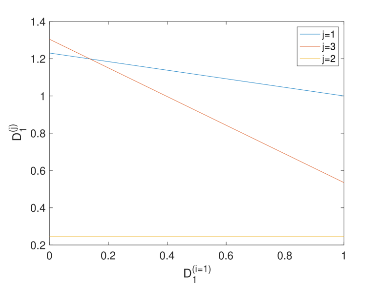
Figure 1: Parametric solution of eqs. (30,31,32) for “possible” values of the partial dimensions of the “folded-towel” map coupled with a bistable linear system. See details in the main text.

3 Minimal models for rough basin boundaries

In order to clarify some of the previous findings, we present here some mathematical toy models of interest.

3.1 Simple rough boundary

A minimal model for bistable systems with ‘uncomplicated’ cross-boundary and ‘complicated’ in-boundary dynamics can be constructed as follows:

$$x_{n+1} = ax_{n}+d(y_{n}-1/2),$$ (33)

$$y_{n+1} = \mu\min(y_{n},1-y_{n}),\ \mu=1+\exp(c|x_{n}|).$$ (34)

Loosely speaking, the cross-boundary dynamics is governed (dominated) by a linear equation (33), and the in-boundary dynamics is a chaotic process produced by a noninvertible 1D map, the tent map (34) in this example. Since the tent map is noninvertible, the whole 2D ($D=2$) system is noninvertible. The coupling is bidirectional. The in-to-cross-boundary coupling is additive, of strength $d$, and the cross-to-in-boundary coupling is multiplicative/parametric through $\mu(x)$. The latter coupling is not needed for a truly minimal model that features a rough basin boundary. The model with $c<0$ can be considered a minimal model for a rough boundary that cannot be described by a (Weierstrass) function $W(y)$. The bistability is between two attractors at $\pm\infty$ wrt. $x$. For our exercise we chose $a=1.1$, $d=0.01$ and $c=-1$.

Given that the perturbation is weak, the LEs of the nonattracting set are approximately those of the unstable fixed point and attractor of the uncoupled bistable and chaotic subsystems, respectively:

$$\lambda_{x}\approx\ln a,\quad\lambda_{y}\approx\ln 2.$$ (35)

Note that small values of $x$ correspond to the nonattracting set embedded in the boundary, and so $\mu\approx 2$ on the nonattracting set.

It can be visually checked in the case of our simple 2D model that the basin boundary is indeed not filamentary, but rather a jagged, rough curve. To this end we initialise many trajectories randomly sprinkled in a box containing the basin boundary, and color small markers placed in these initial positions differently with respect to the different attractor reached. The result of this is shown in Fig. 2.

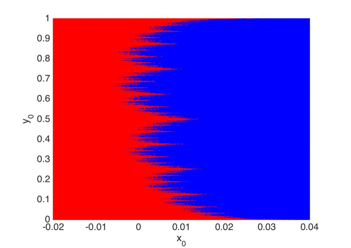
Figure 2: Basins of attraction in the system (33)-(34), depicted by different colours/shades. $2^{22}$ randomly sprinkled initial conditions are used.

This ensemble can be used to check the exponential decaying of the survival rate or probability in the box over time, shown in Fig. 3, by which we can select an exponentially small fraction of the ensemble on the initial configuration that give birth to long-lived trajectories. These initial conditions (IC) are very near the basin boundary, which is the stable manifold of the nonattracting set embedded in it. Therefore, the small fraction of long-lived trajectories should approach the nonattracting set as they evolve (if it is different from the boundary itself—unlike in our case), and then leave the box along the unstable manifold of the nonatracting set. That is, with this procedure, called the sprinkler method [1], one can construct the nonattracting set and its stable and unstable manifolds. Snapshots of the long-lived trajectory ensemble are displayed in Fig. 4, revealing that the stable manifold is identical with the nonattracting set, and that the unstable manifold is space filling. These were indeed the predictions derived from generic dimension formulae in Sec. 2.2 and in Sec. 8.3.1 of [1]. These properties are, again, very different from properties of nonattracting chaotic saddle sets embedded in filamentary fractal basin boundaries of dissipative invertible systems, which saddles have a signature double-fractal geometry, and so their stable and unstable manifolds both consist of filaments, which define two noninteger partial fractal dimensions; see Chapter 6 of [4].

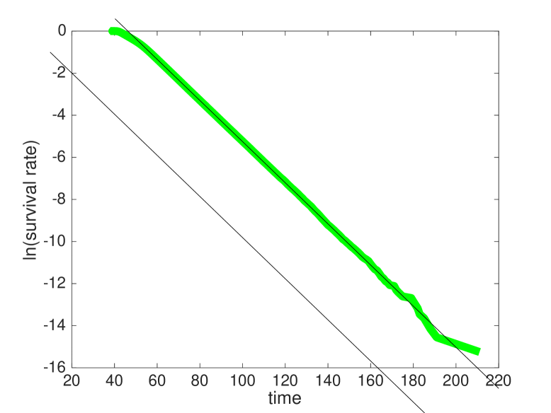
Figure 3: Survival rate based on the initial conditions seen in Fig. 2. The slope on the log-lin diagram gives the escape rate $\kappa$. Parallel straight black lines aid reading off $\kappa$.

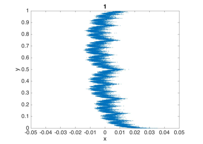
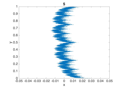
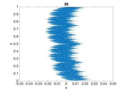
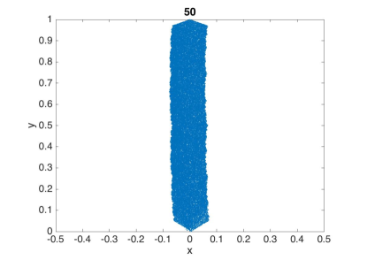
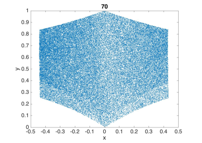
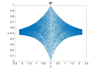
Figure 4: Snapshots from the video following the ensemble used for the sprinkler method applied to the system (33)-(34). Above each panel integer numbers show the iteration number/time passed.

We note that from the survival decay shown in Fig. 3 we can extract the escape rate $\kappa$, which supports our claim that it is just the uncoupled/unperturbed $\tilde{\lambda}_{x}$ given weak perturbations and a regular unperturbed boundary, $\tilde{D}_{1}^{(x)}=0$. On the other hand, the numerically estimated Lyapunov exponents, shown in Fig. 5, also agree with our claim under (35). We estimated the LEs using the Gram-Schmidt procedure. Since the LEs of interest belong to the nonattracting set, we first have to construct that set and its natural measure. It has in fact been already done using the sprinkler method (Fig. 4). The estimates of the LEs at any time are taken as averages of one-step LEs over the ensemble of long-lived trajectories followed.

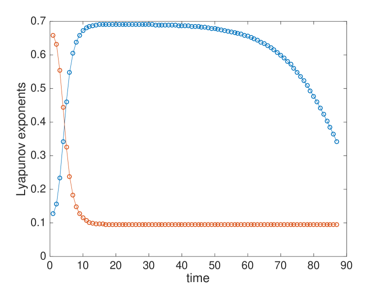
Figure 5: Estimates of the two Lyapunov exponents on the nonattracting set of the system (33)-(34). The actual estimates are those after a transient is past, at about iteration #20. During the transient the Lyapunov (Gram-Schmidt) vector belonging to the blue line turns from a horizontal orientation to a vertical one. The discrete-time data points are linked by straight lines to guide the eye in reading the diagram.

The analytical formulae for the Lyapunov exponents given in [12] for a system similar to (33)-(34) are identical to (35). An analytical formula for the escape rate given in [18] for a generalised model of that in [12] implies for the special case of [12] that the escape rate equals the cross-boundary LE; this is in agreement again with our claim based on our heuristic argument. In [19] the authors derive a formula also for the fractal dimension $D_{b,0}$ which is identical to what we derive from generic relations for the case of weak perturbations as (25) and (27).

In Sec. 4 we check if the said dimension formula applies indeed to our system. We will do this in the invertible 3D ($D=3$) system:

$$x_{n+1} = ax_{n}+d(z_{n}-1/2)$$ (36)

$$y_{n+1} = \left\{\begin{tabular}[]{ll}mod$(2y_{n}+x_{n},1)$&$y_{n}>1/2$\\ mod$(1+2(y_{n}-1)+x_{n},1)$&$y_{n}\leq 1/2$\end{tabular}\right.$$ (39)

$$z_{n+1} = \left\{\begin{tabular}[]{ll}$cz_{n}$&$y_{n}>1/2$\\ $1+c(z_{n}-1)$&$y_{n}\leq 1/2$\end{tabular}\right.$$ (42)

where the linear equation (36) (identical with eq. (33)) is perturbed by the invertible chaotic baker map (39)-(42). The behaviour wrt. the basin boundary is similar (results not shown) as in the 2D noninvertible system (33)-(34). We will use $c=1/3$. However, note that the fractal dimension of the boundary does not depend on $c$; see eq. (24). This 3D model is a minimal model for an invertible system featuring a rough basin boundary with a dissipative dynamics on the nonattracting chaotic set. The nonattracting set in the invertible system can therefore be called a saddle. In contrast, the dynamics on the nonattracting chaotic set of the 2D minimal model (33)-(34), called a repellor, is not dissipative.

3.2 Mixed filamentary and rough boundary

To have a filamentary fractal unperturbed boundary (or perturbed but not rough), we replace the linear eq. (33) of the cross-boundary dynamics by a nonlinear one similar to that studied in [20]:

$$x_{n+1} = d(y_{n}-1/2)+\left\{\begin{tabular}[]{ll}$a(x_{n}+1/2)-1/2,$&$x_{n}<\gamma,$\\ $-bx_{n},$&$|x_{n}|<\gamma,$\\ $a(x_{n}-1/2)+1/2,$&$x_{n}>-\gamma,$\end{tabular}\right.$$ (46)

$$y_{n+1} = \mu/\beta\min[\mod(y_{n},\beta),\beta-\mod(y_{n},\beta)],\ \mu=1+\exp(c|x_{n}|),$$ (47)

where $\beta=2^{1-q}$, $\gamma=(1-a)/(a+b)/2$, $a>2$ and $b>a/(a-2)$. Following the methodology of Sec. 2.2.3 of [1] applied to a similar but not bistable model, we can derive analytical formulae for the unpertubed LEs:

$$\tilde{\lambda}_{x}=\frac{2b\ln a+a\ln b}{2b+a},\quad\tilde{\lambda}_{y}=q\ln 2,$$ (48)

and a formula also for the unperturbed escape rate:

$$\tilde{\kappa}=\ln\left(\frac{ab}{2b+a}\right).$$ (49)

Of these we need $\tilde{\kappa}$ and $\tilde{\lambda}_{y}$ to predict the co-dimension of a rough boundary, on the one hand, by eq. (26) as:

$$D_{1}^{(y)}\approx 1-\frac{\ln\left(\frac{ab}{2b+a}\right)}{q\ln 2}.$$ (50)

On the other hand, by predicting $\lambda_{x}$ and $\lambda_{y}$, we can predict for what parameter choices do we actually get a rough boundary. Note that for $q=1$ eq. (47) is that of the tent map (34). However, with that choice no valid choices of $a$ and $b$ exist to yield a rough boundary, which is the very reason why we use the “camping” (or “multi-tent”) map (47) instead. For reliable numerical verification of the dimension formula (50) we need as large a contribution $\hat{D}_{1}$ from roughness, given by (28), as possible. Reasonably favorable parameter choices for this objective we have found as: $a=4$, $b=\pi/6+a/(a-2)\approx 2.52$, $c=-1$, $d=0.2$, $q=3$, for which we predict $\lambda_{x}=1.18$, $\lambda_{y}=2.08$, $\kappa=0.11$, $D_{1}^{(y)}=0.947$, $\hat{D}_{1}=0.04$. In Fig. 6 we visualize the boundary, providing successive zooms on the rightmost “filament” in order to expose its roughness. The provided value for $\kappa$ has been checked to apply—to the given approximation—to both the unperturbed and perturbed dynamics, indicating that $d$ is small enough. Yet, it is large enough to make the “filaments” not only rough but seemingly intertwined.

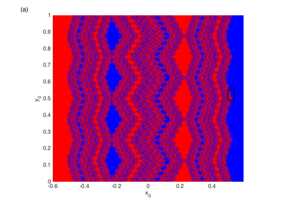
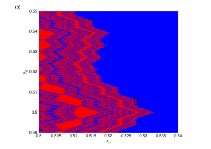
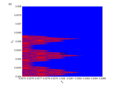
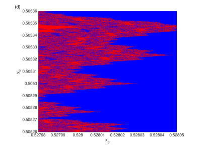
Figure 6: Visual display of a new type of rough basin boundary via the basins of attraction. As in Fig. 2, ICs colored in red (blue) go to the left (right). (a) shows the entirety of the boundary and (b), (c), (d) provide three successive zooms onto features of the rightmost “filament”. The zoomed areas are indicated by black frames.

4 Numerical calculation of the fractal dimension

The co-dimension $D-D_{b,0}$ of the basin boundary is maximum 1, as it has to act as a separator of different regimes of phase space. Because of this, it is possible to determine this co-dimension as the co-dimension $1-D_{0}^{(c)}$ of the intersection set of the boundary and a straight line traversing it. This technique is easily applicable in any high-dimensional system, as demonstrated in [11]. It is important to appreciate that the formula (20) is satisfied for almost any choice of the angle that the traversing line (set $S_{1}$) makes with the boundary (set $S_{2}$), i.e., with probability one for a random choice. Therefore, even if we found that the cross-boundary partial dimension is trivially $D_{0}^{(x)}=1$, applying the said simple method, we will actually measure the nontrivial co-dimension. Therefore, even if we wanted to utilize this distinguishing characteristic of a rough boundary for a detection purpose, we cannot.

On the technical side, it is not immediately clear how to obtain sample points of this intersection set. Instead, the co-dimension can supposedly be determined, being equal to the uncertainty exponent $\alpha$, based on data generated as follows. We populate a $y,z=constant$ line by equispaced ICs, and let them evolve under (36)-(42) until they approach one of the attractors, determining thereby the outcome. A visual representation of the outcomes along the line is given in Fig. 7. It is accompanied by a complicated and seemingly discontinuous function of the lifetimes of the trajectories depending on the ICs, shown in Fig. 8.

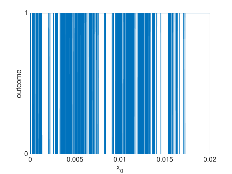
Figure 7: The trajectory of (36)-(42) escapes to positive (negative) infinity wrt. $x$ when the outcome is 1 (0). $2^{17}$ equally spaced ICs of $x_{0}$ are examined in the shown range, while $y_{0}$, $z_{0}$ are fixed at some arbitrary values.

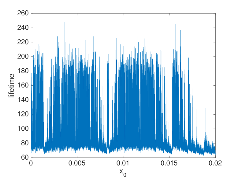
Figure 8: Trajectory lifetimes in (36)-(42) belonging to initial conditions $x_{0}$ (and $y_{0}$, $z_{0}$ fixed at some arbitrary values). $2^{25}$ equally spaced ICs of $x_{0}$ are examined in the shown range.

The ratio $N/N_{0}$ of uncertain boxes, in which we have different outcomes, of linear size $\epsilon$ is shown in Fig. 9. Values of $N/N_{0}$ are plotted on a logarithmic scale, and those of $\epsilon$ are on a linear scale. In the diagram two regimes can be seen, in both of which the decay is exponentially fast, only the scale (the slope in the log-lin diagram) is different. That is, the decay is faster than the usual polynomial decay that defines the uncertainty exponent [1]: $N/N_{0}\sim\epsilon^{\alpha}$. Indeed, plotting in a log-log diagram, seen in Fig. 10, the data does not show a scaling of good quality in any range; the line is curved. The significance of this experience as a negative result is that this alone (without the theory presented in Sec. 2.1) could call into question whether the basin boundary has a fractal geometry as we know it in our case. Next, we proceed with the alternative method by which we could actually verify the fractality of the set and our prediction for the dimension.

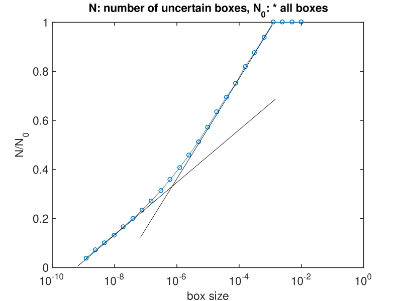
Figure 9: Number of uncertain boxes derived from the initial conditions examined in Fig. 8 versus the linear box size $\epsilon$ in a log-lin diagram. Straight black lines indicate regimes. The discrete data points are linked by straight lines to guide the eye in reading the diagram.

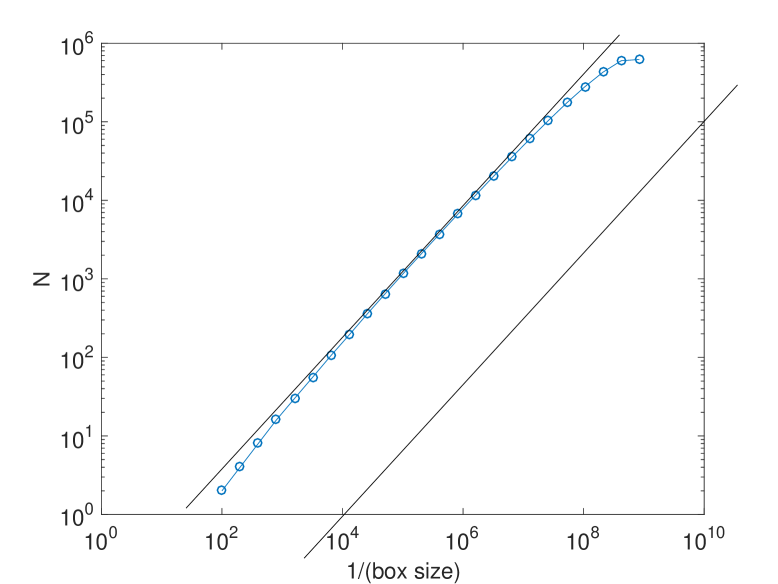
Figure 10: Number of uncertain boxes derived from the initial conditions examined in Fig. 8 versus the linear box size $\epsilon$ in a log-log diagram. Parallel straight black lines indicate the steepness of the slope.

One can apply ‘formally’ a box-counting algorithm to the outcome data to estimate the information dimension $D_{1}^{(c)}$, as if the points where the outcome is reversed by a small shift of the IC corresponded to trajectory data points. The information $I(\epsilon)=-\sum P_{i}(\epsilon)\ln P_{i}(\epsilon)$, $P_{i}$ being normalised box counts [4], as a function of the box size, or rather $-\ln(\epsilon)$, is shown in Fig. 11. This features a scaling of good quality, which, first, verifies fractality (beyond visuals), and, second, we estimate that $D_{1}^{(c)}=0.84$. However, this estimate of the information dimension is appropriate only if the measure across the line over the supporting set is a Lebesgue measure, i.e., constant, because the outcome data does not contain information on the dynamics, only the geometry of the nonattracting set. We have already seen evidence in Fig. 4 that the measure is constant, namely, that the ensemble does not change with respect to its uniform distribution initially, achieved by random sprinkling; the distribution remains uniform. This backs the intuition that the constant measure of the uncoupled chaotic dynamics is inherited by the coupled dynamics. Therefore, $D_{1}^{(c)}=D_{0}^{(c)}$. This agrees with the authors of [18] whose “numerical computation indicates that for the repeller, the box-counting dimension $D_{0}$ and the information dimension $D_{1}$ are equal”, as also noted in Sec. 8.3.1.2 of [1]. This fact has a relevance to the verification of dimension formulae given in Sec. 2, where $D_{1}$ appears instead of $D_{0}$, and if the measure is not uniform, with the above technique we can determine only $D_{0}$. What matters here is that we measure $D_{0}^{(c)}=D_{0}^{(y)}=0.84$, and this numeric value agrees very well with our prediction by eq. (27) being $D_{0}^{(y)}=0.86$.

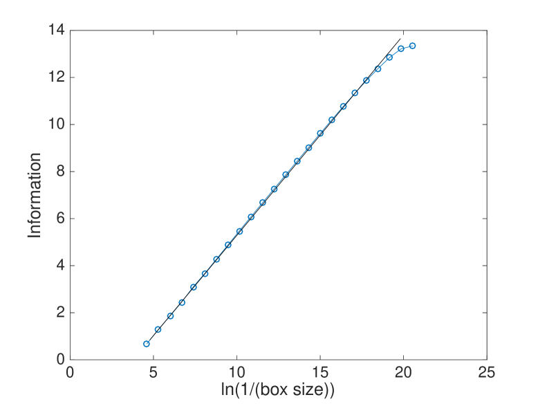
Figure 11: The information derived from the initial conditions examined in Fig. 8 versus the linear box size $\epsilon$. A straight black line indicate the quality of the scaling. The slope of the fitted straight line by least-squares is 0.84, and the room-mean-square-error of the fit is 0.04.

Using the same method we have computed the partial dimension $D_{0}^{(y)}$ of the new type of rough basin boundary featured by (46)-(47), too. Our result of 0.943 with a 0.007 root-mean-square-error of fitting a straight line to data is in rather good agreement with our prediction of $D_{1}^{(y)}=0.947$, even when considering that the contribution from roughness was predicted to be $\hat{D}_{1}=0.04$. Note that the roughness can be resolved only at sufficiently small length scales due to the weakness of the perturbation, as prompted also by Fig. 6.

5 Discussion and outlook

This work has been motivated by the finding of a fractal basin boundary in Ref. [11] in a model whose bistable ocean component is not chaotic. There we conjectured that the condition for rough fractals established by Grebogi et al. [12] in a 2D noninvertible map should apply. Here we show—following the approach of Vollmer et al. [13]—that it is really the case. Furthermore, we derived a formula (24) for the co-dimension of this fractal basin boundary, which is a generalization of the Kantz-Grassberger (KG) formula holding only for filamentary fractal boundaries. We also found that this new formula implies unexpected properties of rough fractals, contrasting those of filamentary fractal boundaries, including the new three-way relationship of the predictability of the second kind and local and global instability. We continue discussing these now.

We speculate that the formal result of $D_{1}^{(x)}=1$, which is not excluded by us to hold also in higher dimensions, owes perhaps to the fact that the boundary as a Weierstrass function is nondifferentiable and continuous in the same time. However, given that it is a function $W(y)$, the dimension $D_{1}^{(c)}$ of the intersection set of the boundary and a straight line $y,z=constant$ is actually 0. We have checked this numerically with $c=0$ in (33)-(34). With two-way coupling, e.g. $c=-1$, we immediately have a $D_{1}^{(c)}>0$.

In the 2D invertible map that we analyzed in detail, it is, instead, $D_{1}^{(y)}<1$ that is not full-dimensional, suggesting that escape occurs not cross-boundary, but along the $y$-direction. The intuitive picture that can be attached to this is that a trajectory has to be “pushed” in the $y$-direction into the “crevices” of the rough boundary “landscape” (into the gaps of the Cantor set whose fractal dimension is $D_{1}^{(y)}$) to be able to escape eventually in the $x$-direction. Although the local directionality of the rough boundary is undefined, its partial dimensions can be associated more directly to the maximal and cross-boundary Laypunov exponents, both of which can be defined without a reference to directions, in an operational manner. The latter is important insomuch that we can check if the condition $\lambda_{x}<\lambda_{U}$ for roughness is satisfied. The cross-boundary LE $\lambda_{x}$, on the one hand, can be defined by the divergence of ensembles initialised according to the natural measure of the nonattracting set, on the two sides very near the boundary, say, in terms of the ensemble means. The MLE $\lambda_{U}$, on the other hand, can also be measured by the divergence of trajectory-pairs (as done in [11]). The difference between these definitions of $\lambda_{x}$ and $\lambda_{U}$ is the opposite order of A) measuring the difference and B) taking the ensemble averages wrt. the natural measure supported by the nonatracting set.

We are not aware of a method by which the formal results of $D_{1}^{(x)}=1$ and $D_{1}^{(y)}<1$ can be verified. By traversing the basin boundary with a line and evaluating the uncertainty exponent of the resulting intersection set, owing to eq. (20), it is not necessarily the partial dimension $D_{1}^{(x)}$ that we can measure, but the always nontrivial co-dimension $D-D_{b,1}$. Therefore, from a practical point of view, as far as the predictability of the second kind alone is concerned, it makes no difference if the basin boundary is a filamentary or a rough fractal. Conversely, we cannot identify the type of fractal by measuring fractal dimensions. We conclude that it can only be identified by measuring both the maximal Lyapunov exponent, as done in [11], and the cross-boundary Lyapunov exponent, upon which the theoretical condition (Sec. 2.1) can be checked. We have done this for our prototype model (46)-(47) featuring a new type of rough boundary, using the ensemble shown in Fig. 4, and show the results in Fig. 12. Given that the ensembles are of finite size, initially no exponential separation can be seen. The separation rate yielded by large values of $\ln d$, that is, when the ensembles departed substantially from the nonattracting set, is $\ln a$, and it clearly does not pertain to the nonattracting set for which eq. (48) predicts the correct value to be $\lambda_{x}\approx 1.18$. We drew a line of that slope into the diagram and find that the initial separation rate (at small values of $\ln d$) is clearly consistent with it. Therefore, the technique proposed for identifying the type of fractal seems to be viable. While a visual identification is possible only in 2D or perhaps 3D systems, the computation of the two LEs should not be hindered by large dimensionality.

We also emphasize that our prediction of the dimension (26) assumes small perturbations; but the condition for roughness has no such assumption. Otherwise, our new eq. (24), the generalization of the Kantz-Grassberger relation (KG), indicates that the ratio of $\lambda_{x}$ and $\lambda_{U}$ not only determines the type of the fractal, but has a bearing also on its dimension. These LEs associated respectively with weather and climatic process in our model in [11] resulted in an almost completely space filling basin boundary, i.e., a complete unpredictability of the outcome on fine scales.

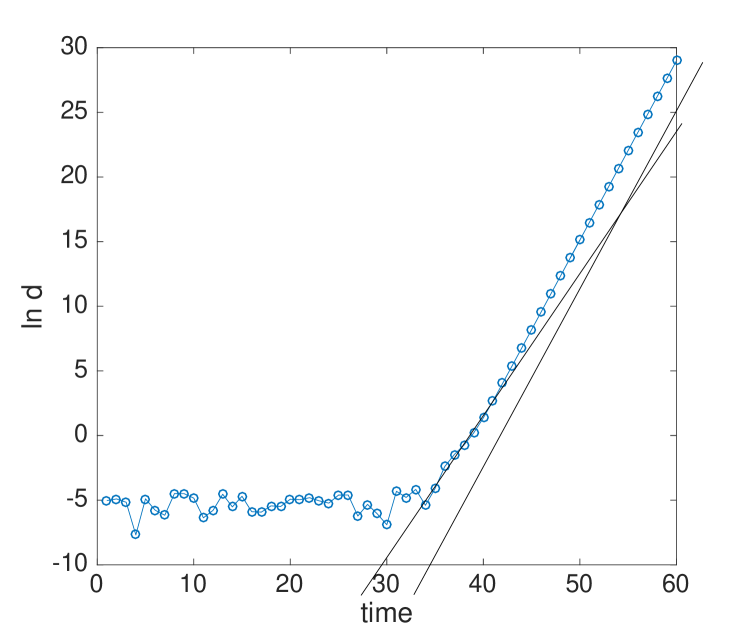
Figure 12: Distance of ensemble means as time progresses, where the two ensembles comprise trajectories with opposite outcomes, as shown in Fig. 4. Straight black lines of slopes $\ln 4\approx 1.39$ and $\lambda_{x}=1.18$ aid the interpretation of the diagram.

Because of the inapplicability of KG, point (ii) of Sec. 1 is not universally valid. Indeed the local and global instabilities can coincide [compare eqs. (24) and (27)], i.e., the fractality due to roughness does not necessarily weaken global instability (in proportion with the co-dimension) like in the case of filamentary fractals. However, we note that when e.g. the roughening happens through perturbation, there could be a weakening of global instability according to the effect first reported in [10] and also examined e.g. in [22], whereby the maximal effect occurs for some nontrivial perturbation strength $\epsilon_{X}$. In contrast, (i.a) remains valid when the boundary is readily rough (when the $X$ subsystem itself maybe a coupled/perturbed system). (i.b), on the other hand, is not necessarily valid, as roughening the boundary by perturbation might change only the fractal dimension of the boundary but not the global instability, as already said. When the global instability is altered by perturbation according to [10] and [22], however, it should contribute to ‘further’ change in the dimension similarly to filamentary fractals [2]. The latter, of course, falls under the validity of (i.a), when the parameter in question can be taken to be the perturbation strength, $p=\epsilon_{X}$.

The decoupled ocean dynamics in [11] was given by a diffusive energy balance model, the Ghil-Sellers model [23], studied also in [14], whose solution is not chaotic, and so the fractality of the basin boundary in the coupled model came only from roughness. In a state-of-the-art Earth system model, or even in an intermediate complexity model with a dynamical ocean like the Planet Simulator atmospheric model coupled to the Goldstein ocean-sea ice model [24], we expect a mixed filamentary-rough fractal basin boundary to be present. It is also clear that due to the vast atmospheric vs climatic time scale separation the basin boundary is practically space filling. However, the answers to two related questions of geophysical relevance are not immediately clear:

• With a realistic Earth-like setup, at what length scale (in phase space) can we resolve the space-filling roughness?

• Is the atmospheric perturbation strong enough to significantly alter the global instability as in [10, 22, 2]?

In a different approach, atmospheric perturbations of the slow climatic model components can be viewed as noise perturbations, possibly inducing transitions or exits from one persistent state to another. Key questions concern the most likely path of transition as well as the expected residence time in the persistent state [25, 26]. These properties are governed by a potential-like quantity [1]. An efficient algorithm is proposed in Ref. [27] to estimate the potential barrier height from controlled exit time data.

References

- [1] Y.-C. Lai and T. Tél. Transient Chaos. Springer, New York, 2011.
- [2] Tamás Bódai, Eduardo G. Altmann, and Antonio Endler. Stochastic perturbations in open chaotic systems: Random versus noisy maps. Phys. Rev. E, 87:042902, Apr 2013.
- [3] Celso Grebogi, Steven W. McDonald, Edward Ott, and James A. Yorke. Final state sensitivity: An obstruction to predictability. Physics Letters A, 99(9):415 – 418, 1983.
- [4] T. Tél and M. Gruiz. Chaotic Dynamics. Cambridge University Press, Cambridge, 2006.
- [5] Francesco Ginelli, Hugues Chaté, Roberto Livi, and Antonio Politi. Covariant lyapunov vectors. Journal of Physics A: Mathematical and Theoretical, 46(25):254005, jun 2013.
- [6] H. Kantz and P. Grassberger. Repellers, semi-attractors, and long-lived chaotic transients. Physica D: Nonlinear Phenomena, 17(1):75 – 86, 1985.
- [7] Jeroen Wouters and Valerio Lucarini. Disentangling multi-level systems: averaging, correlations and memory. Journal of Statistical Mechanics: Theory and Experiment, 2012(03):P03003, mar 2012.
- [8] Jeroen Wouters and Valerio Lucarini. Multi-level dynamical systems: Connecting the ruelle response theory and the mori-zwanzig approach. Journal of Statistical Physics, 151(5):850–860, 2013.
- [9] David Ruelle. A review of linear response theory for general differentiable dynamical systems. Nonlinearity, 22(4):855, 2009.
- [10] Marek Franaszek. Influence of noise on the mean lifetime of chaotic transients. Phys. Rev. A, 44:4065–4067, Sep 1991.
- [11] Valerio Lucarini and Tamás Bódai. Edge states in the climate system: exploring global instabilities and critical transitions. Nonlinearity, 30(7):R32, 2017.
- [12] Celso Grebogi, Edward Ott, and James A. Yorke. Fractal Basin Boundaries, Long-Lived Chaotic Transients, and Unstable-Unstable Pair Bifurcation. Phys. Rev. Lett., 50:935–938, Mar 1983.
- [13] Jürgen Vollmer, Tobias M. Schneider, and Bruno Eckhardt. Basin boundary, edge of chaos and edge state in a two-dimensional model. New Journal of Physics, 11(1):013040, 2009.
- [14] Tamás Bódai, Valerio Lucarini, Frank Lunkeit, and Robert Boschi. Global instability in the Ghil–Sellers model. Climate Dynamics, 44(11):3361–3381, Jun 2015.
- [15] Brian R. Hunt, Edward Ott, and James A. Yorke. Fractal dimensions of chaotic saddles of dynamical systems. Phys. Rev. E, 54:4819–4823, Nov 1996.
- [16] Benoit B. Mandelbrot. A Class of Multinomial Multifractal Measures with Negative (Latent) Values for the “Dimension” f(), pages 3–29. Springer US, Boston, MA, 1989.
- [17] O.E. Rossler. An equation for hyperchaos. Physics Letters A, 71(2):155 – 157, 1979.
- [18] David Sweet and Edward Ott. Fractal dimension of higher-dimensional chaotic repellors. Physica D: Nonlinear Phenomena, 139(1):1 – 27, 2000.
- [19] James L. Kaplan, John Mallet-Paret, and James A. Yorke. The Lyapunov dimension of a nowhere differentiable attracting torus. Ergodic Theory and Dynamical Systems, 4(2):261–281, 006 1984.
- [20] BAE-SIG PARK, CELSO GREBOGI, and YING-CHENG LAI. Abrupt dimension changes at basin boundary metamorphoses. International Journal of Bifurcation and Chaos, 02(03):533–541, 1992.
- [21] Y. Robin, P. Yiou, and P. Naveau. Detecting changes in forced climate attractors with Wasserstein distance. Nonlinear Processes in Geophysics, 24(3):393–405, 2017. cited By 0.
- [22] Eduardo G. Altmann and Antonio Endler. Noise-enhanced trapping in chaotic scattering. Phys. Rev. Lett., 105:244102, Dec 2010.
- [23] Michael Ghil. Climate Stability for a Sellers-Type Model. Journal of the Atmospheric Sciences, 33(1):3–20, 1976.
- [24] P. B. Holden, N. R. Edwards, K. Fraedrich, E. Kirk, F. Lunkeit, and X. Zhu. PLASIM–GENIE v1.0: a new intermediate complexity AOGCM. Geoscientific Model Development, 9(9):3347–3361, 2016.
- [25] Valerio Lucarini and Tamás Bódai. Transitions across melancholia states in a climate model: Reconciling the deterministic and stochastic points of view. Phys. Rev. Lett., 122:158701, Apr 2019.
- [26] Valerio Lucarini and Tamás Bódai. Global Stability Properties of the Climate: Melancholia States, Invariant Measures, and Phase Transitions. arXiv:1903.08348.
- [27] Tamás Bódai. An efficient algorithm to estimate the potential barrier height from noise-induced escape time data. arXiv:1808.06903.