Selection of highly-accreting quasars

Abstract

Context. The quasar class of extreme Population A (xA) (also known as super-Eddington accreting massive black holes, SEAMBHs) has been hailed as potential distance indicators for cosmology.

Aims. The aim of this paper is to define tight criteria for their proper identification starting from the main selection criterion $R_{\rm FeII}$$>1$, and to identify potential intruders not meeting the selection criteria, but nonetheless selected as xA because of the coarseness of automatic searches. Inclusion of the spurious xA sources may dramaticaly increase the dispersion in the Hubble diagram of quasars obtained from virial luminosity estimates.

Methods. We studied a sample of 32 low-$z$ quasars originally selected from the SDSS DR7 as xA or SEAMBHs that have been proved to be almost certainly misclassified sources. All of them show moderate-to-strong Feii emission and the wide majority strong absorption features in their spectra are typical of fairly evolved stellar populations. We performed a simultaneous fit of a host galaxy spectrum, AGN continuum, FeII template and emission lines to spectra, using the fitting technique based on ULySS, full spectrum fitting package. We derive the main accretion parameters (luminosity, black hole mass, and Eddington ratio) and investigate the relation between host galaxy properties and AGN.

Results. For sources in our sample (of spectral types corresponding to relatively low Eddington ratio), we found an overall consistency between H$\beta_{\rm NC}$, [Oiii]$\lambda\lambda$4959,5007 line shifts and the mean stellar velocity obtained from the host galaxy fit (within $\lesssim|60|$  km s${}^{-1}\,$). Non-xA AGN should be distinguished from true xA sources on the basis of several parameters, in addition to the ones defining the Main Sequence spectral type: H$\beta$   asymmetry, unshifted [Oiii]$\lambda\lambda$4959,5007, and the intensity ratio between broad and narrow component of H$\beta$  emission line. Only one source in our sample qualify as xA source.

Conclusions. Correct classification of spectra contaminated by heavy absorption requires careful determination of the host galaxy spectrum. The contamination/misclassification is not usual in the identification of the xAs, nor at low z neither at high z. We found high fraction of host galaxy spectrum (in half of the sample even higher then 40%). When absorption lines are prominent, and the fraction of the host galaxy is high, SSP is mimicking FeII, and that may result in a mistaken identification of FeII spectral features. We have identified several stellar absorption lines that, along with the continuum shape, may lead to an overestimate of $R_{\rm FeII}$, and therefore to the misclassification of sources as xA sources.

1 Introduction

Quasars show properties that make them potential cosmological probes: they are plentiful, very luminous, and detected at very early cosmic epochs (currently out to redshift 7). However, they have never been successfully exploited as distance indicators in the past decades. Their luminosity is spread over six orders of magnitude, making them antithetical to conventional standard candles. Attempts at providing one or more parameters tightly correlated with luminosity were largely unsuccessful in the past decades (i.e., the “Baldwin effect” did not live up to its cosmological expectations (Popović & Kovačević 2011, e.g.,; Bian et al. 2012, e.g.,; Ge et al. 2016, e.g.,, see also Sulentic et al. 2000a for a synopsis up to 1999). Even the next generations of supernova surveys are unlikely to overcome the redshift limit at $\sim 1.5$ (Hook, 2013). At the time of writing there is no established distance indicator in the range of redshift $1.5\lesssim z\lesssim 4$, where important information could be gained on the cosmic density of matter and on the dynamic nature of the dark energy (e.g., D’Onofrio & Burigana, 2009, and references therein).

Realistic expectations are now kindled by isolating a class of quasars with some constant property from which the quasar luminosity can be estimated independently of its redshift. For instance, the non-linear relation between UV and X ray luminosity has been used to build the Hubble diagram up to redshift $\approx$ 5.5 (Risaliti & Lusso, 2015, 2019). Other approaches are being tested as well (e.g., Watson et al., 2011, see also Czerny et al. 2018 for a recent review). A promising possibility is provided by quasars that are accreting at high (possibly super-Eddington) rates (Wang et al., 2014b). Physically, in a super-Eddington accretion regime, a geometrically and optically thick structure known as a “thick disk” is expected to develop (Abramowicz et al., 1988). The accretion flow remains optically thick so that radiation pressure “fattens” it. When the mass accretion rate becomes super-Eddington, the emitted radiation is advected toward the black hole, so that the source luminosity increases only with the logarithm of accretion rate. In other words, the radiative efficiency of the accretion process is expected to decrease, yielding an asymptotic behavior of the luminosity as a function of the mass accretion rate (Abramowicz et al., 1988; Mineshige et al., 2000; Watarai et al., 2000; Sadowski, 2011). In observational terms, the luminosity-to-black hole mass ratio ($L$/$M_{\rm BH}$$\propto$ $L/L_{\rm Edd}$) should tend toward a well-defined value. As the accretion rate increases above $\approx 0.1$, the disk may become first “slim” and then “thick” in supercritical regime (Abramowicz & Straub, 2014, and references therein). The resulting “thick” accretion disk is expected to emit a steep soft and hard X-ray spectrum, with hard X-ray photon index (computed between 2 and 20 KeV) converging toward $\Gamma_{\mathrm{hard}}\approx 2.5$ (Wang et al., 2013). Observationally, results are less clear. There is a broad consensus that the soft X-ray slope and the index $\alpha_{\mathrm{oX}}$ depend on Eddington ratio and can be steep at high accretion rate (Boller et al., 1996; Wang et al., 1996; Sulentic et al., 2000b; Dewangan et al., 2002; Grupe et al., 2010; Bensch et al., 2015). In the hard X-ray domain data on weak-lined quasars which are believed to be all xAs (Martínez-Aldama et al., 2018) suggest weakness, but not necessarily with a steep slope (Shemmer et al., 2010; Ni et al., 2018), possible because the X-ray emission is seen through a dense outflow. More powerful X-ray instrumentation than presently available is needed for accurate derivation of the hard-X continuum shape of sources that are anyway X-ray weak compared to the general population of quasars (Brightman et al., 2019). Quasars hosting thick disks should radiate at a well-defined limit because their luminosity is expected to saturate close to the Eddington luminosity (hence the attribution of “extremely radiating quasars”) even if the mass accretion rate becomes highly super-Eddington (Mineshige et al., 2000). Their physical and observational properties are only summarily known. However, our ability to distinguish sources in different accretion states has greatly improved thanks to the exploitation of an empirical correlation set known as the “main sequence” (MS) of quasars (Boroson & Green, 1992; Sulentic et al., 2000a, b).

The MS concept originates from a principal component analysis carried out on the spectra of $\approx$ 80 Palomar-Green (PG) quasars by Boroson & Green (1992). These authors identified a first eigenvector dominated by an anticorrelation between the [Oiii]$\lambda$5007 peak intensity and the strength of optical Feii emission. Along E1 FWHM of H$\beta$  and Feii prominence are also correlated (Fig. 9 of Boroson & Green 1992), and define a sequence based on optical parameters which are easily measurable on single-epoch spectra of large samples of quasars.

The Eigenvector 1 (E1) in a parameter space of four dimensions (4DE1, Sulentic et al. 2000a, b, 2007) is especially useful to isolate different spectral types and, among them, spectral type that may be associated with extreme phenomena. 4DE1 involves optical, UV and X-ray. Its dimension (1) the full width at half maximum of H$\beta$ , FWHM (H$\beta$ ), 2) the ratio of the equivalent widths of Feii emission at 4570 Å and H$\beta$ , $R_{\rm FeII}$= W (Feii$\lambda$4570) / W (H$\beta$ ) $\approx F$ (Feii$\lambda$4570) / $F$ (H$\beta$ ). (1) and (2) define what has come to be known as the optical plane of E1 quasars main sequence (MS); 3) the photon index in the soft X-rays domain, $\Gamma_{\mathrm{soft}}$, and 4) the blueshift of the high ionization line Civ$\lambda$1549Å . Sulentic et al. (2000a) proposed two main populations on the basis of the quasar systematic trends in the optical plane (FWHM(H$\beta$ ) vs $R_{\rm FeII}$) of the 4DE1 parameter space: Population A for quasars with FWHM (H$\beta$ ) $<$ 4000  km s${}^{-1}\,$ and Population B for those with FWHM (H$\beta$ )$>$ 4000  km s${}^{-1}\,$. The two populations are not homogenous and they show trends in spectral properties, especially within Pop. A (Sulentic et al., 2002). For this reason, the optical plane of E1 was divided into $\Delta$FWHM (H$\beta$ ) = 4000  km s${}^{-1}\,$ and $\Delta$ $R_{\rm FeII}$= 0.5. This defined the A1, A2, A3, A4 bins as $R_{\rm FeII}$ increases, and the B1, B1 +, B1 ++ defined as FWHM (H$\beta$ ) increases (see Figure 1 of Sulentic et al. 2002). Similarly, B2, B2+ and so on for each interval of the 2 strip, with $R_{\rm FeII}$ in the range 0.5 – 1. Thus, spectra belonging to the same bin are expected to have fairly similar characteristics concerning line profiles and optical and UV line ratios (Sulentic et al., 2007; Zamfir et al., 2010). The MS may be driven by Eddington ratio $L/L_{\rm Edd}$ convolved with the effect of orientation (e.g. Boroson, 2002; Ferland et al., 2009; Marziani et al., 2001; Shen & Ho, 2014; Sun & Shen, 2015), although this view is not void of challenges. Physically, quasars may be distinguished by differences in Eddington ratio (mainly the horizontal axis as for A1,A2,A3, etc.) or by orientation (mainly the vertical axis for a fixed black hole mass).

Quasars are considered high accretors (hereafter xA quasars, for extreme Population A quasars) following the work of Marziani & Sulentic (2014, hereafter MS14), if they satisfy the selection criterion:

$$R_{\mathrm{FeII}}=\frac{EW(\mathrm{FeII}\lambda 4570)}{EW(H\beta)}>1.0$$ (1)

At low redshift, we can identify xA quasars following the method described in (MS14), i.e. by isolating sources that have $R_{\rm FeII}$$\geq 1$ i.e., belonging to spectral types A3 and A4, or to bins B3 and B4 if FWHM (H$\beta$ )$>$ 4000  km s${}^{-1}\,$. Super-Eddington accretors can be identified from $\Gamma_{\mathrm{soft}}$ and from the $\Gamma_{\mathrm{hard}}$ (2-20 keV) as well (Wang et al., 2013, 2014b). This method requires deep spectral observations from space-borne instrumentation, and at present, cannot be applied to large samples. The MS of quasars offers the simplest selection criterion $R_{\rm FeII}$$>1$. A similar selection criterion has been defined through the fundamental plane of accreting black holes (Du et al., 2016b), a relation between Eddington ratio (or dimensionless accretion rate), and $R_{\rm FeII}$ and the $D$ parameter defined as the ratio between the FWHM and the dispersion $\sigma$ of the H$\beta$  line profile ($FWHM/\sigma(H\beta)$) (Du et al., 2016b). The fundamental plane can be written as two linear relations between $\log\dot{\cal M}$ and $L_{\rm bol}/L_{\rm Edd}$ versus $\approx\alpha+\beta\frac{\rm FWHM}{\sigma}+\gamma R_{\rm FeII},$ where $\alpha(>0),\beta(<0),\gamma\ (>0)$ are reported by Du et al. (2016b). The values of Eddington ratio and $\dot{{\mathcal{M}}}$ derived from the fundamental plane equation are large enough to qualify the xA sources satisfying $R_{\rm FeII}$$>1$ as SEAMBHs. The converse may not be true, since some SEAMBHs have been identified that corresponds to spectral types A2 and even A1 (e.g. Mrk 110). The point is that A1 and A2 show the minimum value of $D$ as their H$\beta$  most closely resemble Lorentzian functions while in A3 and A4 a blue-shifted excess leads to an increase in $D$. In the following we will consider $R_{\rm FeII}$$>1$  (or 1.2 if doubtful borderline cases have to be excluded, following Negrete et al. 2018, hereafter Paper I) as a necessary condition to consider a source xA or SEAMBH, with the two terms.

As mentioned, accretion theory supports the empirical finding of MS14 on xA sources. First, $L/L_{\mathrm{Edd}}\sim{\cal O}(1)$ (up to a few times the Eddington luminosity) is a physically motivated condition. The ability to obtain a redshift independent distance then stems from the knowledge of the $L/L_{\rm Edd}$ with a small dispersion around a characteristic value, and from the ability to estimate the black hole mass ($L/L_{\rm Edd}$$\propto$ L/$M_{\rm BH}$). The preliminary analysis carried out in the last two years (e.g. Paper I) emphasize the need to avoid the inclusion of “intruders” in the Hubble diagram build from xA, as they can significantly increase the dispersion in the distance modulus.

In this paper, we take advantage of the sample of quasars in Paper I that were selected from an automatic analysis, and we focus on the sources that were affected by strong contamination of the host galaxy and that turned out not to be xA sources. The identification of large samples of xA sources needed for their cosmological exploitation is and will remain based on surveys collected from fixed apertures or, at best, diffraction limited PSFs $\approx 0.1$ arcsec, as in the case of Euclid (Euclid Red Book Editorial Team, 2011). Therefore, the broad line emitting regions will be always unresolved, and contaminated by emission from regions more distant from the central continuum source. Specifically, a major role is played by the host galaxy stellar spectrum. We will therefore devote the paper to a detailed study of the emission properties and of the host spectrum of the “intruders” in order to better define exclusion criteria.

Section 2 describes the method followed for the sample selection. The merit of the sample is to provide sources covering a relatively wide range of $R_{\rm FeII}$ with typical low-luminosity type-1 properties, for which several intriguing properties of the host galaxy and of the AGN can be measured for the same object: age and chemical compositions as well as radial velocity shifts of narrow emission lines associated with the AGN narrow line region (NLR). In addition, the host galaxy spectrum effect on the appearance of the AGN spectrum can be thoroughly analysed. We then describe several approaches aimed at obtaining the spectroscopic components associated with the AGN continuum and the emission spectrum (Section 3). Section 4 provides measurements and results on the host spectrum, internal line shifts (analysing in detail the use of the [Oii]$\lambda$3727 doublet whose rest frame wavelength is dependent on electron density), and narrow and broad emission line parameters. Section 5 discusses the results in the context of the quasar main sequence, trying to assess the main factors affecting the $M_{\rm BH}$ and $L/L_{\rm Edd}$ estimates in small samples. In Section 6 are reported main conclusions and a summary of the paper.

2 Sample selection

The quasar sample presented by Shen et al. (2011) consists of 105,783 quasar spectra of the SDSS DR7 and was vetted following several filters: $z<0.8$ to cover the range around H$\beta$ and include the Feii$\lambda$4570 and 5260 Å blends; (2) S/N$>$ 20. Only 2,734 spectra satisfy these criteria, reduced to 468 with (3) $R_{\rm FeII}$$\geq$ 1. S/N and $R_{\rm FeII}$ were estimated through the automatic measurements after continuum normalization at 5100 Å. Then we measured the EW of FeII and H$\beta$  in the ranges 4435-4686 and 4776-4946 respectively (Boroson & Green, 1992) to estimate $R_{\rm FeII}$. Among the 468 sources Negrete et al. (2018) found 134 of them whose spectra are either noisy or are of the intermediate type (Sy $\sim$ 1.5), that is, the emission of the broad component of H$\beta$  is very weak compared to its narrow component, which is usually intense. These authors excluded them to a have a final sample of 334 sources properly classified as type 1 with $R_{\rm FeII}$$\gtrsim 1$. Thirty-two of 334 sources showed strong contamination from the host galaxy. It turned out that the host-galaxy contamination mimicked the Feii emission features customarily found around H$\beta$ , leading to an overestimate of $R_{\rm FeII}$ from the automated measurement (see 4.3). The study of this sample (hereafter HG) is presented in this paper, while the rest of the sample (which we found out is in part suited for our cosmological project) has been in an independent paper devoted to the exploitation of xA quasars for cosmological parameter estimates (Paper I).

Table 1 reports the identification, the redshift, the $g$ magnitude, the color index $g-r$, the specific flux at 6cm in mJy (FIRST), the log of the specific flux at 2500Å, and the radio-loudness parameter $R=f_{\nu}(6\mathrm{cm})/f_{\nu}$(2500Å) (Jiang et al., 2007; Kellermann et al., 1989). According to Jiang et al. (2007) radio sources are classified as radio-quiet for $R\leq 10$, and radio-loud for $R>10$. Data reported in Table 1 are taken from the table of Shen et al. (2011), where radio properties are included by matching SDSS DR7 quasar with the FIRST White et al. (1997). The radio fluxes densities are subject to a considerable uncertainty (to be a factor of $\approx$2 from a coarse analysis on the FIRST maps): the sources are faint, the continuum are extrapolated from 20cm to 6cm using a power-law with index 0.5, and affected by reduction residuals in the maps. The radio power is actually modest; in the case of SDSSJ151600.39+572415.7 at $z\approx 0.2$, $\log P_{\nu}[W/Hz]\approx 30.4$ , which is typical of radio detected sources in spectral type A2 (Ganci et al., 2019) to which this source belongs. Similar considerations apply to the other two sources. On the basis of the results of Ganci et al. (2019), the three sources may not be even truly RL source in the sense of having a relativistic jet (Padovani, 2017).

Table 1: Basic properties of the HG sample

SDSS ID	$z$	$g$	$g-r$	$f$(6cm)	$\log f$(2500Å)	R
(1)	(2)	(3)	(4)	(5)	(6)	(7)
J003657.17-100810.6	0.19	17.84 $\pm$ 0.02	0.34 $\pm$ 0.03		-26.89
J010933.91+152559.0	0.23	18.97 $\pm$ 0.02	0.44 $\pm$ 0.04		-27.24
J011807.98+150512.9	0.32	19.16 $\pm$ 0.02	0.47 $\pm$ 0.04		-27.19
J031715.10-073822.3	0.27	19.08 $\pm$ 0.03	0.56 $\pm$ 0.05		-26.93
J075059.82+352005.2	0.41	19.37 $\pm$ 0.02	0.24 $\pm$ 0.03		-27.14
J082205.19+584058.3	0.31	19.48 $\pm$ 0.02	0.46 $\pm$ 0.04		-27.21
J082205.24+455349.1	0.30	18.38 $\pm$ 0.02	0.44 $\pm$ 0.04		-27.02
J091017.07+060238.6	0.30	19.13 $\pm$ 0.04	0.68 $\pm$ 0.05		-27.06
J091020.11+312417.8	0.26	18.73 $\pm$ 0.01	0.42 $\pm$ 0.03		-27.07
J092620.62+101734.8	0.27	19.25 $\pm$ 0.02	0.55 $\pm$ 0.03		-27.53
J094249.40+593206.4	0.24	18.88 $\pm$ 0.02	0.46 $\pm$ 0.04		-27.19
J094305.88+535048.4	0.32	19.18 $\pm$ 0.03	0.48 $\pm$ 0.05		-27.16
J103021.24+170825.4	0.25	18.63 $\pm$ 0.02	0.39 $\pm$ 0.03		-27.19
J105530.40+132117.7	0.18	17.61 $\pm$ 0.02	0.22 $\pm$ 0.04		-26.64
J105705.40+580437.4	0.14	17.66 $\pm$ 0.05	0.37 $\pm$ 0.07		-26.87
J112930.76+431017.3	0.19	18.46 $\pm$ 0.03	0.60 $\pm$ 0.04		-27.37
J113630.11+621902.4	0.21	18.72 $\pm$ 0.02	0.49 $\pm$ 0.05		-27.06
J113651.66+445016.4	0.12	17.71 $\pm$ 0.04	0.59 $\pm$ 0.05	1.95	-26.97	18.3
J123431.08+515629.2	0.30	19.05 $\pm$ 0.03	0.54 $\pm$ 0.05	1.07	-27.42	27.9
J124533.87+534838.3	0.33	18.51 $\pm$ 0.03	0.36 $\pm$ 0.05		-27.08
J125219.55+182036.0	0.20	18.98 $\pm$ 0.02	0.79 $\pm$ 0.03		-27.18
J133612.29+094746.8	0.25	19.10 $\pm$ 0.02	0.49 $\pm$ 0.04		-27.33
J134748.06+404632.6	0.27	19.17 $\pm$ 0.02	0.82 $\pm$ 0.03		-27.28
J134938.08+033543.8	0.20	18.70 $\pm$ 0.03	0.53 $\pm$ 0.05		-27.16
J135008.55+233146.0	0.27	18.14 $\pm$ 0.02	0.23 $\pm$ 0.05		-27.00
J141131.86+442001.0	0.26	18.90 $\pm$ 0.03	0.61 $\pm$ 0.04		-27.18
J143651.50+343602.4	0.30	19.22 $\pm$ 0.01	0.35 $\pm$ 0.04		-27.44
J151600.39+572415.7	0.20	18.41 $\pm$ 0.02	0.58 $\pm$ 0.04	2.27	-26.96	20.4
J155950.79+512504.1	0.24	18.82 $\pm$ 0.02	0.39 $\pm$ 0.04		-27.26
J161002.70+202108.5	0.22	18.80 $\pm$ 0.02	0.61 $\pm$ 0.03		-27.25
J162612.16+143029.0	0.26	19.71 $\pm$ 0.02	0.88 $\pm$ 0.03		-27.62
J170250.46+334409.6	0.20	18.14 $\pm$ 0.01	0.41 $\pm$ 0.02		-27.10

Notes: (1) SDSS name, (2) redshift, (3) $g$ magnitude, (4) color index $g-r$, (5) specific flux at 6cm in mJy (= $10^{-26}$ erg s^-1 cm^-2 Hz^-1), (6) log of the specific flux per unit frequency at 2500Å, in erg s^-1 cm^-2Hz^-1, (7) radio-loudness parameter $R\equiv f_{\nu}(6\mathrm{cm})/f_{\nu}$(2500Å) Jiang et al. (2007).

3 Data analysis

In Paper I we have found subsample of 32 sources with strong contamination by host galaxy. That analysis was done using specfit (Kriss, 1994). Here we made data analysis using technique based on ULySS (Koleva et al., 2009a). Results are compared with two separate techiques. One based on specfit and STARLIGHT, and another one based on DASpec. Since we obtained fairly consistent result with all techiques, we made more detailed analysis only with ULySS, such as Monte Carlo simulations and $\chi^{2}$ maps. Therefore, all results presented in tables and on figures are done with ULySS.

3.1 ULySS - Full Spectrum Fitting

The analysis was performed using ULySS, a full spectrum fitting software package, that we adopted for fitting Sy1 spectra with models representing a linear combination of non-linear model components – AGN continuum, host galaxy, Feii template and emission lines. The detailed description is given in (Bon et al., 2016), where ULySS has been used for the first time for fitting Sy 1 spectra.
Before running the fitting procedure we converted vacuum wavelengths into air, using the IAU definition Morton (1991), since the wavelength calibration of the SDSS spectra is in Heliocentric vacuum wavelength, while the components of the model are in air wavelengths. Therefore, all analysis were done in air wavelengths.

Line and continuum fittings

We adjusted ULySS to analyze simultaneously all components that contribute to the flux in the wavelength region $\lambda\lambda=[3700,6800]\AA$. The model that we used for the fit represents bounded linear combination of non-linear components - (i) stellar population spectrum, convolved with a line-of-sight velocity broadening function, (ii) an AGN continuum model represented with a power law function, (iii) a sum of Gaussian functions accounting for AGN emission lines in analysed spectral domain, and (iv) Fe II template.
In order to eliminate overall shape differences between the observed stellar and galactic spectra, the model is multiplied by a polynomial function that is a linear combination of Legendre polynomials. The introduction of this polynomial in the fit ensures that results are insensitive to the Galactic extinction, normalization and the flux calibration of a galaxy and stellar template spectra (Koleva et al., 2008). The polynomial is replacing the prior normalization to the pseudo-continuum that other methods need. We have used a third order of the polynomial in the fit, in order to model at best the extinction function, and at the same time to prevent that the higher order terms of the polynomial affect the fit of broad emission lines and AGN continuum.
The single stellar population spectra (SSP) used for the fit of the host galaxy are spline interpolated over an age-metallicity grid of stellar population models from the library of SSPs computed by Vazdekis (1999) with the Miles library (Sánchez-Blázquez et al., 2006).
Emission lines are fitted with the sum of Gaussians in the following way:
(i) all Balmer lines, as well as HeII are fitted with four components - narrow, two broad components that fit the wings of the lines and very broad component;
(ii) to tie widths, shifts and intensities of the [O III] lines, we defined two separate components of the model - a narrow component and a semi-broad component. Intensity ratio was kept to 3:1 (Dimitrijević et al., 2007);
(iii) the rest of emission lines are mainly fitted with two Gaussians - for the fit of narrow and semi-broad component. Eventhough in some cases the fit was possible with smaller number of Gaussian components, in order to stay consistent and perform the analysis in the same way for all spectra, we used for the whole sample the same number of components.
We used the semi-empirical FeII template by Marziani et al. (2009), obtained from a high resolution spectrum of I Zw 1 starting from 4000 Å. In the range underlying the H$\beta$  profile the FeII emission was modeled with the help of FeII emission from the photoionization code CLOUDY version 07.01 (Ferland et al., 1998).

The AGN model is generated with the same sampling and at the same resolution as the observations, and the fit is performed in the pixel space. The fitting method consists of a non-linear minimization procedure for minimizing the $\chi^{2}$ between an observed spectrum and a model. The fitting procedure applies the Levenberg-Marquardt minimization technique (Marquardt, 1963). The coefficients of the multiplicative polynomial are determined by least-squares method at each evaluation of the function minimized by the Marquardt-Levenberg routine. As well, at each iteration the weight of each component is determined using a bounding value least-square method (Lawson & Hanson, 1995).
The simultaneous fit of all components in the model, that implies as well the simultaneous analysis of kinematic and evolutionary parameters of the stellar population, minimizes in a most efficient way many degeneracies between AGN model components reported in the literature, such as: (i) degeneracy between fractions of AGN continuum and the host galaxy (Bon et al., 2014; Moultaka, 2005), (ii) SSP age-metallicity degeneracy (Koleva et al., 2009a), and (iii) degeneracy between stellar velocity dispersion and SSP metallicity (Koleva et al., 2009b).

4 Results

4.1 Immediate SSP and spectral classification results

The results of the host galaxy single population analysis with ULySS are reported in Table 2. The table lists, after the SDSS ID (Col. 1) the specific flux measured at 5100 $\AA$ (as proposed by Richards et al. 2006), the light fraction of power law continuum, and the power law spectral index (Cols. 3-4). Cols. 5-8 report information on the SSP analysis: the light fraction of the host galaxy, the SSP age, and the SSP shift with respect to the rest frame defined by the SDSS-provided redshift value. The shift of the H$\beta$ narrow component (H$\beta_{\rm NC}$) and of narrow [OIII]$\lambda$5007 line are reported in Cols. 9–10. The shift and width (the Gaussian dispersion $\sigma$) of FeII lines are listed in Col. 11 – 12. Cols. 13–16 list the flux and $\sigma$ for H$\beta_{\rm NC}$ and [OIII]$\lambda$5007. Fig. 13 in Appendix A shows a spectral atlas with the main components.

Classification concerning spectral type assignment along the E1 MS optical diagram and AGN classification according to Véron-Cetty & Véron (2006) are presented in Table 3. The Table lists: the FWHM and Flux of H$\beta_{\rm BC}$ (Cols. 2-3), $R_{\rm FeII}$ and the main sequence spectral type (Cols. 4-5), along with the classification of the Catalogue of Véron-Cetty & Véron (2006). Sources for which no classification is given in the Catalogue are recognizable as type-1 AGN in the SDSS (from S1.0 to 1.8). However, the classification of some of them (for example J162612.16) might not have been easy on old spectroscopic data, right because of the strong host contamination. Cols. 7 to 8 list the FWHM H$\beta_{\rm BC}$ and $R_{\rm FeII}$ following Shen et al. (2011). The corresponding spectral type is listed in Col. 9. The last columns report, in this order, the FW at 1/4, 1/2, 3/4 and 0.9 H$\beta_{\rm BC}$ peak intensity, and the H$\beta_{\rm BC}$ centroid at quarter and half maximum, $c(\frac{1}{4})$ and $c(\frac{1}{2})$. These parameters are useful in the asymmetry and the shift analysis, especially at 1/4 of maximum intensity. Both H$\beta$  and [Oiii]$\lambda\lambda$4959,5007 are often affected by asymmetries close to the line base. The 1/4 maximum intensity provides a suitable level to detect and quantify these asymmetries.

4.2 Spectral Type Classification along the quasar MS: not xA sources in almost all cases

The HG sample sources remain by all measurements relatively strong Feii emitters, with $R_{\rm FeII}$$\gtrsim 0.3$. Fig. 1 shows the location of the 32 sources in the optical plane of the E1 MS (represented with red and blue circles). The $R_{\rm FeII}$ and FWHM H$\beta$  place the sources predominantly into the B2 and A2 spectral bins; only one source can be considered genuine xA candidate.

There is good agreement between our measurements of $R_{\rm FeII}$ and those of Shen et al. (2011): from the measurements reported in Table 2, $R_{\rm FeII}$ (Shen et al. 2011) $\approx(1.07\pm 0.08)$$R_{\rm FeII}$+ ($0.18\pm 0.06$), implying that Shen et al. (2011) values are systematically higher by 18%. The reason for this disagreement could be that Shen et al. (2011) did not take into account the host galaxy contribution (Śniegowska et al., 2018). This analysis would imply that 5/32 sources could be classified as xA with $R_{\rm FeII}$$>$1, following Shen et al. (2011). The number reduces to only 1 out of 32 if the most restrictive criterion $R_{\rm FeII}$$\geq 1.2$ is applied. Parameter $D=FWHM_{H\beta}/\sigma_{H\beta}$  distinguishes sources on the Fig. 1 in two groups. Sources with $D>1.5$ show a more Gaussian-like H$\beta$ profile. $D<1.5$ implies a more Lorenzian-like profile.

As mentioned above, only one source (SDSS J105530.40+132117.7) is confirmed as xA in the full HG sample after SSP analysis, applying the selection criterion $R_{\rm FeII}$ $\gtrsim 1.2$. This source will be individually discussed in §5. The restriction to $R_{\rm FeII}$$\geq 1.2$ is operational, to avoid contamination from a fraction of borderline objects that may not be really xA: since typical uncertainties are $\delta$$R_{\rm FeII}$$\approx$0.1 at 1$\sigma$ confidence level, the presence of “imitators” should be reduced by 95% the number expected with the limit at $R_{\rm FeII}$=1. Therefore, source SDSS J105530.40+132117.7 should be considered true xA and analysed as such at a confidence level $\gtrsim 4\sigma$.

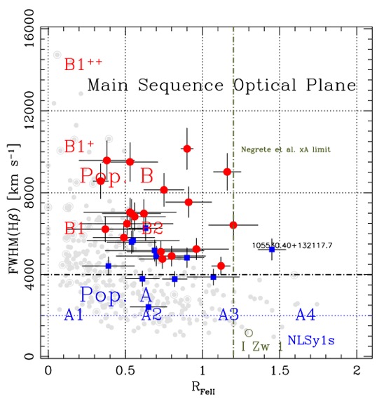
Figure 1: The optical plane of the E1 MS, FWHM H$\beta_{\rm BC}$ vs $R_{\rm FeII}$. Sources from our sample are represented as red and blue circles; the grey symbols represent the MS from the sample of Zamfir et al. (2010), with RL sources identified by an outer circle. The red circles are sources with the $D$ parameter larger than 1.5; for the blue squares $D\lesssim 1.5$. The horizontal dot-dashed line marks the limit between Population A and at FWHM $=$ 4000  km s${}^{-1}\,$. Dotted lines separate spectral types and NLSy1s. The vertical dot-dashed olive line identifies the $R_{\rm FeII}$=1.2 limit for xA “safe” identification according to Paper I. Only one source qualifies as a true xA candidates. The position of the prototypical xA source I Zw 1 is marked.

Table 2: Measurements of the host galaxy, AGN continuum, and emission lines parameters with ULySS.

SDSS ID	$f_{\lambda}$(5100)	AGN $f$	sp. index	SSP $f$	SSP age	SSP $cz$	SSP $\sigma_{\star}$	H$\beta_{\mathrm{NC}}$ z	OIII $z$	FeII $z$	FeII $\sigma$	H$\beta_{\mathrm{NC}}$ $\sigma$	H$\beta_{\mathrm{NC}}$ flux	[OIII] $\sigma$	[OIII] flux
	[$10^{-17}$erg/s/cm${}^{2}/$Å]	[%]		[%]	[Myr]	[ km s${}^{-1}\,$]	[ km s${}^{-1}\,$]	[ km s${}^{-1}\,$]	[ km s${}^{-1}\,$]	[ km s${}^{-1}\,$]	[ km s${}^{-1}\,$]	[ km s${}^{-1}\,$]	[$\star\star$]	[ km s${}^{-1}\,$]	[$\star\star$]
(1)	(2)	(3)	(4)	(5)	(6)	(7)	(8)	(9)	(10)	(11)	*(12)	(13)	(14)	(15)	(16)
J003657.17-100810.6	29.74	46.8 $\pm$ 0.3	-0.66 $\pm$ 0.23	44.0 $\pm$ 0.2	5398 $\pm$ 469	60 $\pm$ 9	196 +/- 10	-8 $\pm$ 20	38 $\pm$ 6	288 $\pm$ 173	1635 $\pm$ 143	189 $\pm$ 26	2.80 $\pm$ 0.01	155 $\pm$ 10	6.21 $\pm$ 0.15
J010933.91+152559.0	10.87	50.9 $\pm$ 0.7	-0.04 $\pm$ 0.15	38.6 $\pm$ 0.7	4445 $\pm$ 905	119 $\pm$ 15	138 +/- 17	4 $\pm$ 26	95 $\pm$ 29	30 $\pm$ 174	1492 $\pm$ 227	138 $\pm$ 31	1.86 $\pm$ 0.36	129 $\pm$ 40	1.45 $\pm$ 0.58
J011807.98+150512.9	10.02	55.8 $\pm$ 0.6	-0.25 $\pm$ 0.05	34.5 $\pm$ 0.6	6649 $\pm$ 245	-40 $\pm$ 20	170 +/- 22	-60 $\pm$ 17	-43 $\pm$ 7	252 $\pm$ 62	1375 $\pm$ 252	119 $\pm$ 19	1.87 $\pm$ 0.04	139 $\pm$ 11	5.01 $\pm$ 0.66
J031715.10-073822.3	12.87	64.3 $\pm$ 0.6	-0.81 $\pm$ 0.04	27.3 $\pm$ 0.6	1595 $\pm$ 329	170 $\pm$ 16	104 +/- 20	132 $\pm$ 11	145 $\pm$ 11	88 $\pm$ 97	1953 $\pm$ 799	145 $\pm$ 12	3.84 $\pm$ 0.28	102 $\pm$ 15	2.55 $\pm$ 0.17
J075059.82+352005.2	6.91	59.1 $\pm$ 0.4	-1.25 $\pm$ 0.06	33.5 $\pm$ 0.5	1431 $\pm$ 89	66 $\pm$ 10	95 +/- 14	107 $\pm$ 18	104 $\pm$ 5	232 $\pm$ 138	1302 $\pm$ 155	129 $\pm$ 21	1.75 $\pm$ 0.23	153 $\pm$ 6	7.86 $\pm$ 0.22
082205.19+584058.3	8.00	69.2 $\pm$ 0.6	-0.25 $\pm$ 0.20	22.5 $\pm$ 0.6	6252 $\pm$ 477	-7 $\pm$ 26	127 +/- 31	-45 $\pm$ 24	68 $\pm$ 13	568 $\pm$ 65	2256 $\pm$ 497	47 $\pm$ 24	0.82 $\pm$ 0.06	134 $\pm$ 19	3.74 $\pm$ 0.50
082205.24+455349.1	17.47	77.4 $\pm$ 0.4	-0.79 $\pm$ 0.01	13.7 $\pm$ 0.3	3493 $\pm$ 194	60 $\pm$ 21	100 +/- 27	-5 $\pm$ 24	-3 $\pm$ 14	252 $\pm$ 106	1273 $\pm$ 89	76 $\pm$ 29	0.52 $\pm$ 0.52	186 $\pm$ 16	0.00 $\pm$ 0.44
091017.07+060238.6	12.22	50.3 $\pm$ 0.3	-2.00 $\pm$ 0.00	42.5 $\pm$ 0.3	3037 $\pm$ 74	154 $\pm$ 11	116 +/- 13	99 $\pm$ 56	66 $\pm$ 12	176 $\pm$ 208	1408 $\pm$ 248	170 $\pm$ 70	0.86 $\pm$ 0.11	161 $\pm$ 20	4.59 $\pm$ 0.13
091020.11+312417.8	13.89	60.0 $\pm$ 0.5	-0.48 $\pm$ 0.11	34.2 $\pm$ 0.5	3434 $\pm$ 52	71 $\pm$ 14	151 +/- 17	73 $\pm$ 15	45 $\pm$ 14	387 $\pm$ 145	1676 $\pm$ 623	147 $\pm$ 19	2.55 $\pm$ 0.10	124 $\pm$ 17	1.91 $\pm$ 0.21
092620.62+101734.8	9.46	47.7 $\pm$ 0.6	-0.12 $\pm$ 0.17	45.5 $\pm$ 0.6	5623 $\pm$ 206	66 $\pm$ 12	142 +/- 15	61 $\pm$ 31	22 $\pm$ 23	872 $\pm$ 105	1310 $\pm$ 251	148 $\pm$ 36	1.70 $\pm$ 0.21	95 $\pm$ 37	1.16 $\pm$ 1.01
094249.40+593206.4	14.30	57.6 $\pm$ 0.5	-0.21 $\pm$ 0.03	35.6 $\pm$ 0.5	5724 $\pm$ 417	84 $\pm$ 12	137 +/- 14	95 $\pm$ 29	39 $\pm$ 33	318 $\pm$ 158	1454 $\pm$ 206	173 $\pm$ 35	1.76 $\pm$ 0.06	135 $\pm$ 35	0.84 $\pm$ 1.96
094305.88+535048.4	9.69	51.4 $\pm$ 0.3	-1.85 $\pm$ 0.04	40.8 $\pm$ 0.3	4428 $\pm$ 352	14 $\pm$ 15	149 +/- 17	35 $\pm$ 32	41 $\pm$ 12	-128 $\pm$ 80	1288 $\pm$ 284	176 $\pm$ 37	1.58 $\pm$ 0.37	154 $\pm$ 24	4.87 $\pm$ 0.64
103021.24+170825.4	16.30	64.1 $\pm$ 0.3	-0.90 $\pm$ 0.09	21.3 $\pm$ 0.3	9363 $\pm$ 290	134 $\pm$ 13	86 +/- 16	173 $\pm$ 38	76 $\pm$ 25	-88 $\pm$ 278	1881 $\pm$ 118	47 $\pm$ 41	0.29 $\pm$ 0.04	212 $\pm$ 68	2.31 $\pm$ 0.17
105530.40+132117.7	38.72	70.4 $\pm$ 0.3	-1.20 $\pm$ 0.03	23.9 $\pm$ 0.2	3072 $\pm$ 246	41 $\pm$ 11	106 +/- 14	-81 $\pm$ 32	93 $\pm$ 17	-215 $\pm$ 213	1701 $\pm$ 200	131 $\pm$ 37	0.72 $\pm$ 0.00	132 $\pm$ 0	2.26 $\pm$ 0.57
105705.40+580437.4	40.27	36.8 $\pm$ 0.5	-0.63 $\pm$ 0.09	55.9 $\pm$ 0.5	1601 $\pm$ 177	51 $\pm$ 9	144 +/- 10	30 $\pm$ 15	-6 $\pm$ 27	253 $\pm$ 143	829 $\pm$ 77	81 $\pm$ 18	1.24 $\pm$ 2.31	130 $\pm$ 40	1.59 $\pm$ 0.98
112930.76+431017.3	20.58	35.2 $\pm$ 0.4	-1.10 $\pm$ 0.16	58.6 $\pm$ 0.3	3333 $\pm$ 159	100 $\pm$ 6	110 +/- 8	87 $\pm$ 26	94 $\pm$ 23	364 $\pm$ 232	1378 $\pm$ 214	139 $\pm$ 31	1.47 $\pm$ 0.24	103 $\pm$ 35	1.19 $\pm$ 0.63
113630.11+621902.4	19.49	55.6 $\pm$ 0.5	-0.89 $\pm$ 0.10	36.4 $\pm$ 0.4	1933 $\pm$ 74	130 $\pm$ 14	143 +/- 16	51 $\pm$ 26	-35 $\pm$ 10	327 $\pm$ 139	2206 $\pm$ 456	171 $\pm$ 33	3.00 $\pm$ 0.01	179 $\pm$ 14	7.16 $\pm$ 0.38
113651.66+445016.4	42.49	36.6 $\pm$ 0.3	-1.13 $\pm$ 0.22	57.1 $\pm$ 0.3	2535 $\pm$ 191	-8 $\pm$ 8	147 +/- 9	-79 $\pm$ 12	67 $\pm$ 14	70 $\pm$ 294	1633 $\pm$ 340	165 $\pm$ 14	3.28 $\pm$ 0.21	84 $\pm$ 22	1.85 $\pm$ 0.38
123431.08+515629.2	11.37	40.4 $\pm$ 0.8	-0.17 $\pm$ 0.29	52.1 $\pm$ 0.8	2838 $\pm$ 408	40 $\pm$ 11	117 +/- 13	44 $\pm$ 12	0 $\pm$ 14	368 $\pm$ 113	1391 $\pm$ 384	31 $\pm$ 0	1.97 $\pm$ 0.37	164 $\pm$ 19	4.48 $\pm$ 0.20
124533.87+534838.3	10.65	53.4 $\pm$ 0.6	-0.71 $\pm$ 0.13	38.3 $\pm$ 0.7	1355 $\pm$ 66	-8 $\pm$ 14	112 +/- 18	34 $\pm$ 22	102 $\pm$ 34	385 $\pm$ 241	1464 $\pm$ 314	107 $\pm$ 28	1.27 $\pm$ 0.09	56 $\pm$ 64	0.28 $\pm$ 0.75
125219.55+182036.0	18.69	61.1 $\pm$ 0.5	-0.14 $\pm$ 0.07	30.9 $\pm$ 0.5	3182 $\pm$ 250	106 $\pm$ 14	142 +/- 16	76 $\pm$ 32	77 $\pm$ 7	204 $\pm$ 156	1457 $\pm$ 208	166 $\pm$ 51	1.77 $\pm$ 0.20	73 $\pm$ 13	2.51 $\pm$ 0.13
133612.29+094746.8	12.96	48.4 $\pm$ 0.6	-0.19 $\pm$ 0.09	43.5 $\pm$ 0.5	6914 $\pm$ 709	79 $\pm$ 15	178 +/- 16	-46 $\pm$ 42	54 $\pm$ 23	337 $\pm$ 106	1324 $\pm$ 179	153 $\pm$ 56	1.16 $\pm$ 0.58	84 $\pm$ 36	1.27 $\pm$ 0.13
134748.06+404632.6	13.72	44.5 $\pm$ 0.4	-0.84 $\pm$ 0.08	49.3 $\pm$ 0.4	4761 $\pm$ 427	122 $\pm$ 15	201 +/- 16	-36 $\pm$ 122	14 $\pm$ 23	926 $\pm$ 88	1430 $\pm$ 386	289 $\pm$ 183	1.14 $\pm$ 0.14	88 $\pm$ 33	0.87 $\pm$ 0.11
134938.08+033543.8	18.60	50.0 $\pm$ 0.3	-1.81 $\pm$ 0.07	44.0 $\pm$ 0.2	5606 $\pm$ 738	90 $\pm$ 13	169 +/- 14	35 $\pm$ 28	73 $\pm$ 10	-71 $\pm$ 250	1656 $\pm$ 339	159 $\pm$ 35	1.91 $\pm$ 0.43	190 $\pm$ 17	6.39 $\pm$ 0.06
135008.55+233146.0	20.82	66.1 $\pm$ 0.3	-0.73 $\pm$ 0.18	22.9 $\pm$ 0.3	3766 $\pm$ 229	80 $\pm$ 15	150 +/- 18	85 $\pm$ 30	13 $\pm$ 15	193 $\pm$ 106	2500 $\pm$ 176	71 $\pm$ 34	0.34 $\pm$ 0.24	214 $\pm$ 16	0.00 $\pm$ 0.03
141131.86+442001.0	15.64	38.1 $\pm$ 0.4	-1.15 $\pm$ 0.15	55.3 $\pm$ 0.4	4704 $\pm$ 719	58 $\pm$ 15	221 +/- 16	21 $\pm$ 44	-14 $\pm$ 5	1321 $\pm$ 148	995 $\pm$ 324	170 $\pm$ 56	1.18 $\pm$ 0.45	139 $\pm$ 6	5.52 $\pm$ 0.08
143651.50+343602.4	8.43	44.4 $\pm$ 0.4	-2.00 $\pm$ 0.00	47.3 $\pm$ 0.3	9489 $\pm$ 1150	4 $\pm$ 21	198 +/- 22	-88 $\pm$ 54	-51 $\pm$ 12	192 $\pm$ 134	1755 $\pm$ 498	203 $\pm$ 62	2.26 $\pm$ 0.68	229 $\pm$ 13	0.00 $\pm$ 1.34
151600.39+572415.7	24.42	35.8 $\pm$ 0.6	-0.22 $\pm$ 0.05	57.6 $\pm$ 0.6	1595 $\pm$ 785	96 $\pm$ 9	172 +/- 11	48 $\pm$ 17	-21 $\pm$ 13	313 $\pm$ 162	1286 $\pm$ 331	170 $\pm$ 22	3.06 $\pm$ 0.21	156 $\pm$ 18	3.13 $\pm$ 0.45
155950.79+512504.1	11.79	63.3 $\pm$ 0.6	-0.19 $\pm$ 0.11	27.8 $\pm$ 0.6	4366 $\pm$ 506	126 $\pm$ 21	152 +/- 24	171 $\pm$ 24	48 $\pm$ 12	224 $\pm$ 179	1488 $\pm$ 235	144 $\pm$ 32	2.00 $\pm$ 0.32	120 $\pm$ 18	4.27 $\pm$ 0.07
161002.70+202108.5	18.09	40.7 $\pm$ 0.6	-0.07 $\pm$ 0.16	50.9 $\pm$ 0.6	3439 $\pm$ 397	79 $\pm$ 9	141 +/- 11	24 $\pm$ 16	-34 $\pm$ 6	291 $\pm$ 126	1316 $\pm$ 178	155 $\pm$ 18	3.24 $\pm$ 0.20	153 $\pm$ 13	9.03 $\pm$ 0.16
162612.16+143029.0	8.57	40.7 $\pm$ 0.6	-0.29 $\pm$ 0.16	48.1 $\pm$ 0.5	11220 $\pm$ 645	112 $\pm$ 16	198 +/- 17	40 $\pm$ 27	435 $\pm$ 21	98 $\pm$ 152	2252 $\pm$ 302	253 $\pm$ 31	3.74 $\pm$ 0.30	138 $\pm$ 30	3.26 $\pm$ 0.17
170250.46+334409.6	20.89	50.8 $\pm$ 0.4	-0.30 $\pm$ 0.30	39.5 $\pm$ 0.3	9704 $\pm$ 392	50 $\pm$ 11	156 +/- 12	108 $\pm$ 36	92 $\pm$ 12	279 $\pm$ 102	1324 $\pm$ 161	161 $\pm$ 48	1.54 $\pm$ 0.05	185 $\pm$ 18	5.65 $\pm$ 0.17

Notes: (1) SDSS ID of the object ; (2) flux measured at 5100 $\AA$ in $10^{-17}$erg/s/cm${}^{2}/$Å(hereafter in the table [$\star\star$]) (Richards et al., 2006); (3) fraction of power law continuum; (4) power law spectral index (errors present 1$\sigma$ dispersion obtained from Monte Carlo simulations); (5) contribution of the host galaxy; (6) SSP age (errors present a dispersion obtained from Monte Carlo simulations); (7) mean stellar velocity; (8) stellar velocity dispersion (9) shift of the H$\beta$ narrow component; (10) shift of narrow [OIII]$\lambda$5007 line; (11) shift of FeII lines; (12) width of FeII lines; (13) width of H$\beta$ narrow component; (14) flux of H$\beta$ narrow component; (15) width of narrow [OIII]$\lambda$5007 component; (16) flux of narrow [OIII]$\lambda$5007 component.

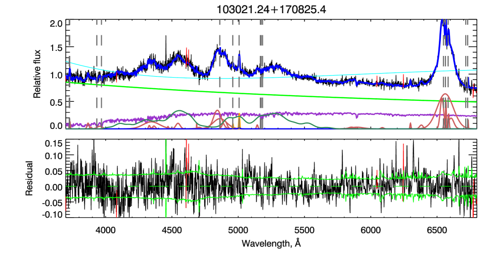
Figure 2: The example of the spectra with strong FeII emission. In the upper panel the black line represents the observed spectrum, blue line the best fit model, and the cyan line represents the multiplicative polynomial, while the green, light red, and violet lines represent components of the ULySS best fit model: violet – stellar population, red – emission lines, and green – AGN continuum. Grey vertical lines mark the wavelengths in the air of the next lines: [OII]3727.5, CaII H & K, H$\beta$ narrow component, [OIII]$\lambda\lambda$4959, 5007 narrow components and MgI b lines, narrow components of H$\alpha$, [NII]$\lambda\lambda$46548,6583 and [SII]$\lambda\lambda$46716,6731, respectively. Residuals from the best fit (black line) are shown on the bottom panel . The dashed line is the zero-axis, and the green solid line shows the level of the noise. Red lines in both panels correspond to outliers of the fit.

(a)

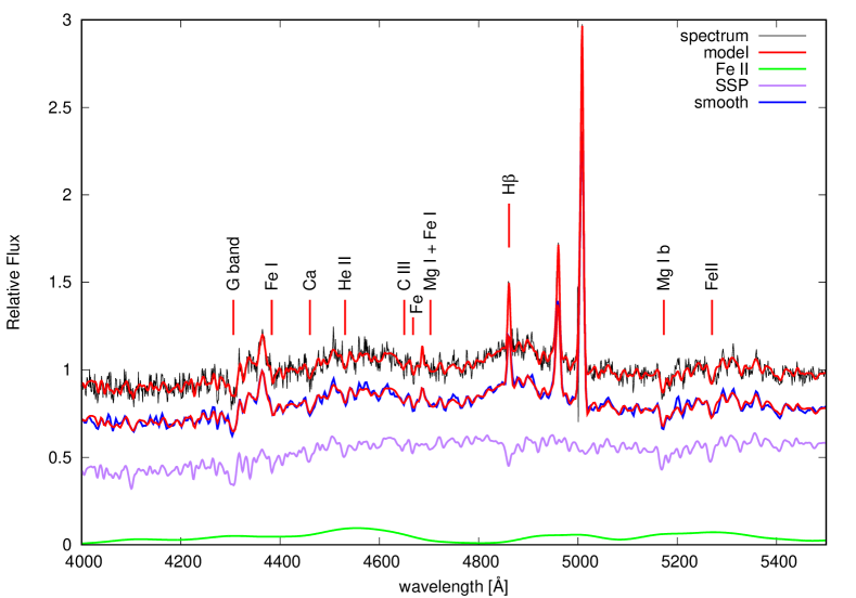
(b)

Figure 3: Examples of spectra (J092620.62+101734.8 and J113651.66+445016.4, respectively) from our sample where the host galaxy mimic strong Feii emission leading to a mistaken identification of strong FeII emitters. Spectra on the plots (a) and (b) have widely different SNR. The panels show (from top to bottom): the real spectra and the best fitting model; the smoothed spectra overlapped with the best fitting model; single stellar population spectra that were used in the best fitting model; and the Feii template used in the fit. Some prominent absorption lines are marked on the plots.

4.3 The reason of the xA misclassification: contamination by host galaxy absorptions

A main issue is why the HG sources were misclassified in the first place. An example of HG spectrum with the various fit components is shown in Fig. 2. We notice the high contribution of the host galaxy spectrum which is a general feature of the sample. Only one source has SSP fraction between 10% and 20% to the total flux. In all other spectra we find very high fraction of the SSP component (in 16 object even higher then 40%). The feature that can be used as an indication of strong contamination from the host galaxy is primarily the MgIb feature that is almost always observed along with H$\beta$  and [Oiii]$\lambda\lambda$4959,5007. When absorption lines are prominent, and the fraction of the host galaxy is high, we detected that SSP is mimicking FeII, and that this may lead to mistaken identification of FeII spectral features (see Fig. 3). As one can see on the Fig. 3, the superposition of high fraction of the SSP on the FeII template, mimics FeII emission lines. This effect is more noticeable in the case of high SNR, as shown on the right hand side of the Fig. 3. The combined effect of the G band at about 4220 Å and the Ca absorption at 4455 Å  creates the impression of an excess emission around 4300 Å, as expected from multiplets m27 and m28 (Feii multiplet wavelengths and information on spectral terms were taken from the Moore 1945 multiplet tables). The CaI absorption apparently delimits the blue side of the $\lambda 4570$ blend, due mostly to the Feii m38 and m37 lines. At the red end of the blend, the CIII 4650
Å , Fe 4668 Å , and FeI absorptions at $4600-4650$ Å help again create illusion of a bump around $\lambda 4570$. The stellar continuum remains relatively flat down to $\approx$ 4400 - 4500 Å, and steepens short-ward; this behavior also contributes to the visual impression of a FeII $\lambda 4570$ emission blend.

Similar considerations apply on the red side of H$\beta$ : the MgIb “green triplet” cuts the continuum between the line of m42 at the blue edge of the blend (at 5169 Å), and the shortest wavelength line of m49 at 5197 Å. The FeI absorption at 5270 Å corresponds roughly to a 5295 Å dip between two pairs of lines of m48 and m49 (5265 Å and 5316 Å, corresponding to the transitions z⁴D${}_{1\frac{1}{2}}^{\mathrm{o}}$   $\rightarrow$ a⁴G${}_{2\frac{1}{2}}$ and z⁴F${}_{4\frac{1}{2}}^{\mathrm{o}}$   $\rightarrow$ a⁴G${}_{5\frac{1}{2}}$: Moore 1945). Again, the Fe I absorption at 5335 Å finds a rough correspondence in the dip at $\approx$5349 Å between two lines of m48 and m49 (at 5316 Å and 5363 Å of m48). Last, at the red end of the $\lambda 5130$ blend, FeI triplet at $\lambda$ 5406 with the possible contribution of the HeII 5412 absorptions, contributes the illusion of significant emission also on the red side of H$\beta$ . This explains the misidentification of the xA sources by the automatic procedure or by a superficial inspection.

In case of a significantly lower dispersion, the strong host contamination creates the appearance of a blue Feii emission blend at $\lambda$4570 much stronger than the red one at $\lambda 5300$, even if the S/N ratio is high. This phenomenon – that can be misinterpreted if the spectral coverage does not extend below 4000 Å in the rest frame – might be responsible for early claims of a different blue-to-red Feii intensity ratio. Fig. 4 illustrates how a spectrum heavily contaminated by the host galaxy, with insufficient spectral coverage and/or dispersion may lead to an incorrect placement of the continuum that in turns implies an anomalous ratio between the Feii blends on the blue and red side. Independently from resolution, little can be said on the spectrum if S/N$\lesssim$10: the G and MgIb bands are lost in noise if they have $W\sim 1$ Å. If the resolution is high, noise can be reduced by filtering, but little can be done in the case of low resolution ($\ll$ 1000). An accurate Feii measurements necessitates of S/N$\sim$30 in the continuum, and of inverse spectral resolution R$\gtrsim$1000 in the case of a significant contamination by the host galaxy spectrum.

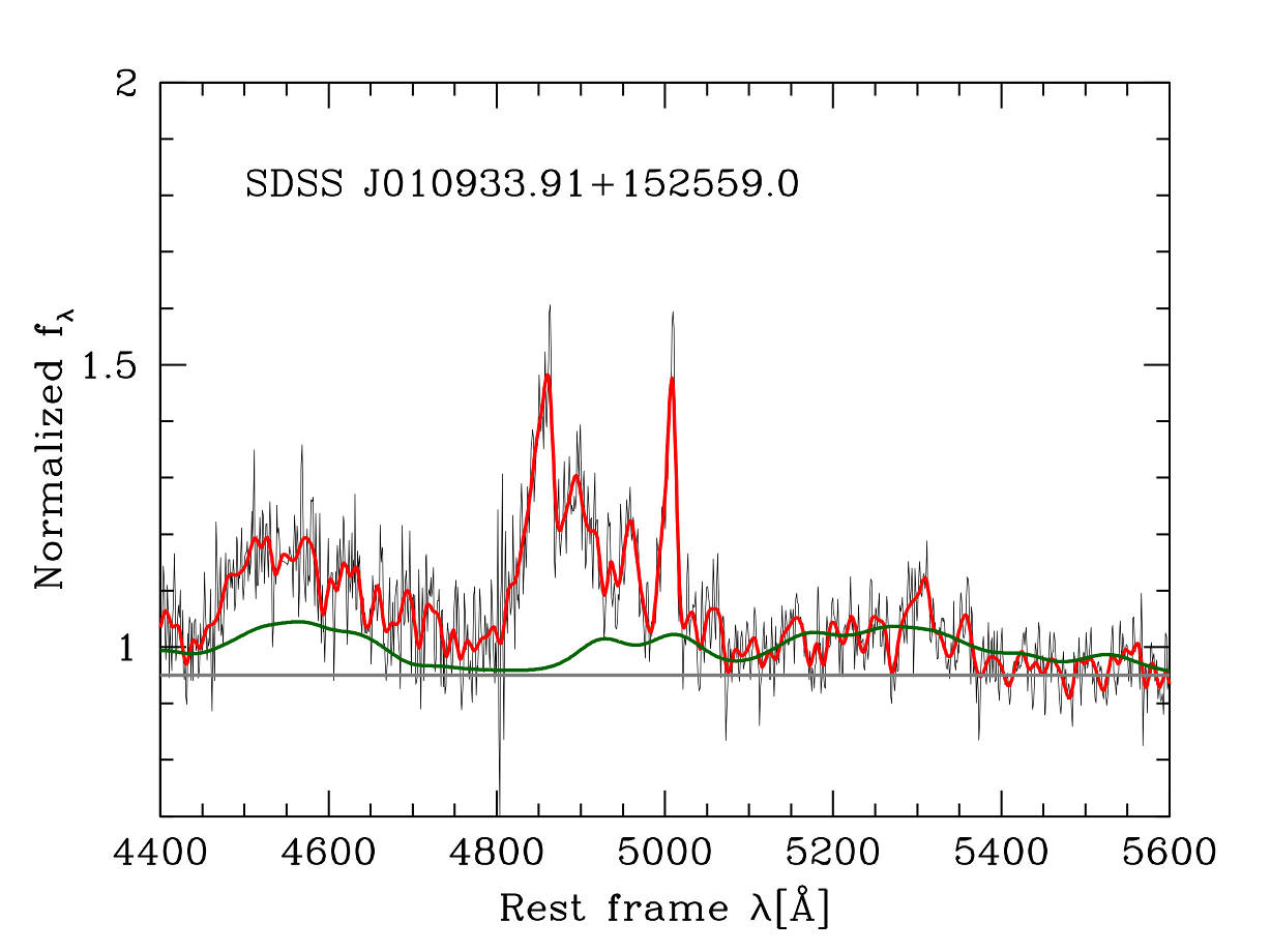
Figure 4: Example of rest-frame spectrum whose features are misinterpreted because of heavy contamination by the absorption spectrum of the host galaxy and because of insufficient spectral coverage. The spectrum is shown with the original SDSS resolution (thin black line) and after rebinning to model data with significantly lower resolution (thick red line). The flat continuum (grey line) erroneously suggests a significant deviation from the Feii template (dark green line).

Monte Carlo simulations (for more information how one can use Monte Carlo simulation with ULySS see (Koleva et al., 2009a)) showed independence between prominence of Feii and SSP fraction, even if we might have expected to find correlation between these two parameters (see Fig. 5, left). Cross correlation also showed lack of dependence between these two parameters (for example, for the case of SDSS J124533.87+534838.3 we found $r=0.13$, $P=7.12E-12$). Besides, we found degeneracies between the age of the dominant stellar population on one hand and the fraction of Feii template and the width of emission lines that make up Feii template on the other, in the sense that we find older stellar populations when we have lower fraction of FeII, and narrower Feii lines (this confirms also Pearson’s cross-correlation which for example for SDSSJ 124533.87+534838.3 gives $r=-0.87$, $P=8E-15$). The Fig. 5 shows just an example; different ages are involved with different objects. Relative age inferences should not be affected, although the simulations show that the actual uncertainty is larger ($\sim 1Gyr$) than the ones reported in Table 2, which are formal uncertainties from the MC simulations. Found degeneracies are not necessarily due to a physical reason, and could be due to the technical fitting problem. In order to decrease degeneracies between parameters of stellar population and FeII template to the minimum, it is advisable to perform the simultaneous fit of these components of the model, as done. This implies that the degeneracies could be even higher in the non-simultaneous fit of the components.

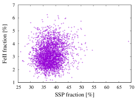
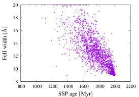
Figure 5: Results of 3000 Monte Carlo simulations for the object SDSSJ124533.87+534838.3 reveal no dependency between SSP and FeII fraction (left), and a degeneracy between SSP age and Feii width (right).

Table 3: Spectral classification.

SDSS ID	FWHM H$\beta_{\mathrm{BC}}$	Flux H$\beta_{\mathrm{BC}}$	$R_{FeII}$	$EV1_{class}$	$AGN_{class}$	FWHM(H$\beta_{\mathrm{BC}})^{\ast}$	$R_{\mathrm{FeII}}^{\ast}$	$EV1_{class}^{\ast}$	FW 1/4	FW 3/4	FW 9/10	C 1/4	C 1/2
(1)	(2)	(3)	(4)	(5)	(6)	(7)	(8)	(9)	(10)	(11)	(13)	(13)	(14)
J003657.17-100810.6	4827	27.1 $\pm$ 2.3	0.9 $\pm$ 0.1	B2	S1	5860	1.1	B3	8634	3104	1933	239	-300
J010933.91+152559.0	4903	36.4 $\pm$ 6.7	0.8 $\pm$ 0.2	B2	S1	4629	0.9	B2	7675	3038	1795	526	166
J011807.98+150512.9	9501	36.7 $\pm$ 5.6	0.5 $\pm$ 0.2	B2+	S1	11091	0.9	B2+	13381	6103	3675	1390	1423
J031715.10-073822.3	8564	28.1 $\pm$ 1.2	0.3 $\pm$ 0.1	B1+	S1	9024	0.8	B2+	12605	4473	2475	1063	198
J075059.82+352005.2	6830	38.8 $\pm$ 4.4	0.6 $\pm$ 0.2	B2	S1	8008	0.8	B2+	10371	5103	1718	541	-141
J082205.19+584058.3	8136	36.7 $\pm$ 4.1	0.8 $\pm$ 0.1	B2+	–	7729	0.9	B2	11652	5171	3102	-316	-311
J082205.24+455349.1	7538	32.8 $\pm$ 4.6	0.9 $\pm$ 0.1	B2	S1	9677	1.2	B3+	11626	5044	3591	800	595
J091017.07+060238.6	7042	32.5 $\pm$ 4.5	0.5 $\pm$ 0.3	B2	AGN	7947	0.7	B2	9888	5592	4695	562	93
J091020.11+312417.8	5807	16.6 $\pm$ 1.2	0.5 $\pm$ 0.2	B1	–	6469	0.7	B2	7120	4770	1170	447	474
J092620.62+101734.8	4906	28.4 $\pm$ 7.0	0.7 $\pm$ 0.3	B2	S1	8350	0.9	B2+	8287	2972	1728	166	320
J094249.40+593206.4	3880	19.9 $\pm$ 0.7	1.1 $\pm$ 0.2	A3	S1	3982	1.2	A3	7252	2219	1318	209	1127
J094305.88+535048.4	9578	34.5 $\pm$ 3.2	0.4 $\pm$ 0.2	B1+	AGN	9457	0.5	B2+	13643	6343	4626	-478	-483
J103021.24+170825.4	6416	50.4 $\pm$ 6.4	1.2 $\pm$ 0.2	B3	–	6285	1.7	B4	8414	4275	2065	-251	-160
J105530.40+132117.7	5228	12.6 $\pm$ 0.7	1.5 $\pm$ 0.1	B3	X	8013	1.8	B4+	7985	3233	1926	-791	-1012
J105705.40+580437.4	2418	26.8 $\pm$ 2.5	0.6 $\pm$ 0.1	A2	–	2826	0.8	A2	3868	1520	898	208	239
J112930.76+431017.3	5176	22.8 $\pm$ 5.2	0.7 $\pm$ 0.3	B2	S1	9154	1.1	B3+	8909	3036	1794	197	-32
J113630.11+621902.4	6982	31.0 $\pm$ 2.1	0.6 $\pm$ 0.1	B2	AGN	7445	0.9	B2	11417	4140	1929	757	447
J113651.66+445016.4	5118	16.6 $\pm$ 2.4	0.7 $\pm$ 0.2	B2	S1	7214	1.1	B3	8099	3181	1867	876	617
J123431.08+515629.2	5662	26.0 $\pm$ 4.9	0.6 $\pm$ 0.3	B2	AGN	8896	0.7	B2+	9765	4005	2970	1019	129
J124533.87+534838.3	6484	33.6 $\pm$ 7.5	0.5 $\pm$ 0.3	B2	AGN	6956	0.7	B2	10050	4353	3043	-802	-207
J125219.55+182036.0	6272	29.5 $\pm$ 2.7	0.6 $\pm$ 0.1	B2	–	7675	0.8	B2	10749	3038	1242	-497	-426
J133612.29+094746.8	5247	26.5 $\pm$ 5.0	1.0 $\pm$ 0.2	B2	–	6556	1.3	B3	7310	3664	1248	-255	80
J134748.06+404632.6	4427	29.3 $\pm$ 3.0	0.4 $\pm$ 0.2	B1	S1	5208	0.5	B1	6638	2837	1730	521	650
J134938.08+033543.8	3781	19.1 $\pm$ 1.1	0.8 $\pm$ 0.1	A2	AGN	3464	1.1	A3	6402	2337	1375	-784	-1208
J135008.55+233146.0	10145	46.0 $\pm$ 1.6	0.9 $\pm$ 0.0	B2+	X	11098	1.2	B3+	14354	6556	4003	-11	-19
J141131.86+442001.0	6219	20.9 $\pm$ 2.0	0.4 $\pm$ 0.2	B1	S1	6779	0.8	B2	7736	4977	3941	207	336
J143651.50+343602.4	6985	32.5 $\pm$ 6.3	0.5 $\pm$ 0.2	B2	S1	7102	0.7	B2	9204	5533	4565	806	583
J151600.39+572415.7	3798	16.6 $\pm$ 0.1	0.6 $\pm$ 0.1	A2	S1	4444	0.6	B2	5666	2555	1519	326	145
J155950.79+512504.1	4765	31.4 $\pm$ 4.0	0.7 $\pm$ 0.2	B2	S1	5593	0.9	B2	7385	1790	964	-29	165
J161002.70+202108.5	4424	19.5 $\pm$ 1.2	1.1 $\pm$ 0.1	B3	–	5080	1.2	B3	6428	2834	1728	416	441
J162612.16+143029.0	9017	31.8 $\pm$ 2.6	1.2 $\pm$ 0.1	B3+	–	9620	1.4	B3+	12665	5783	3511	-805	-803
J170250.46+334409.6	5588	42.7 $\pm$ 4.6	0.5 $\pm$ 0.2	B2	AGN	6528	0.7	B2	10023	3935	2902	444	-137

Notes: (1) SDSS ID of the object; (2) FWHM H$\beta$; (3) F H$\beta$ BC - flux of broad H$\beta$ line component; (4) $R_{FeII}$; (5) classification of the spectra using EV1 diagram; (6) AGN classification according to Véron-Cetty & Véron (2006)–Sy 1 - Seyfert 1 galaxy; – AGN - unclassified AGN; (7) FWHM of broad H$\beta$ from (Shen & Ho, 2014); (8) calculated $R_{FeII}$ using data from (Shen & Ho, 2014); (9) classification of spectra on EV1 diagram, calculated from (Shen & Ho, 2014) data. (10) FW 1/4 - full width of H$\beta$ line; (11) FW3/4 of H$\beta$; (12) FW9/10 H$\beta$; (13) C 1/4 - centroid of H$\beta$ line measured at 1/4 of maximum intensity; (7) C 1/2 - centroid of H$\beta$ line measured at 1/2 of maximum intensity.

4.4 Consistency between AGN emission and host galaxy absorption spectrum

Figure 6: Radial velocity difference between H$\beta_{\rm NC}$ (grey) and [Oiii]$\lambda\lambda$4959,5007 (black) with respect to the HG reference frame.

Generally speaking, there is a good consistency between estimators of the systemic redshift of the host galaxy and low ionization narrow emission lines (a fact known since the early study of Condon et al., 1985). The systemic redshift of the host may be estimated using the atomic 21 cm hydrogen lines or emission from molecular CO which usually give results in close agreement (Mirabel & Sanders, 1988). A third method is provided by the absorption features of the old stellar population of the host galaxies. The tips of the narrow emission line H$\beta$  and H$\alpha$ can be considered the best estimator the system redshift of the host galaxy (Letawe et al., 2007). Significant differences are found mostly for the high ionization lines such as [Oiii]$\lambda\lambda$4959,5007. The agreement between narrow low-ionization lines and the systemic redshift estimators has the important implication that any shift with respect to them can be considered also a shift with respect to the host. This is an advantage as the inter-line shifts between low- and high- narrow ionization lines are easy to measure. The amplitude of the relative shifts is known to depend on the location along the main sequence. In extreme Pop. B shifts between Balmer lines and [Oiii]$\lambda$5007 are generally modest $\lesssim 100$  km s${}^{-1}\,$ (Eracleous & Halpern, 2004). In Pop. B [Oiii]$\lambda\lambda$4959,5007 are often blueward asymmetric close to the line base, but the peak shift is roughly consistent with systemic redshift (see the diagram of average [Oiii]$\lambda$5007 shift along the MS in Marziani et al., 2018). In Pop. A and especially among xAs the [Oiii]$\lambda$5007 shifts become larger, and may reach several hundred  km s${}^{-1}\,$ in the case of the so-called blue outliers (Zamanov et al., 2002; Komossa et al., 2008; Zhang et al., 2011; Cracco et al., 2016; Marziani et al., 2016), believed to be relatively frequent at high Eddington ratio or high luminosity.

Figure 6 shows the radial velocity difference between H$\beta_{\rm NC}$ (grey) and [Oiii]$\lambda\lambda$4959,5007 (black) with respect to the mean stellar velocity reference frame (HG). The comparison shows that 1) both H$\beta$  and [Oiii]$\lambda\lambda$4959,5007 shifts are consistent with HG with some scatter (54  km s${}^{-1}\,$for the case of H$\beta$ and 61  km s${}^{-1}\,$for [OIII]).

The Pearson’s cross-correlation between parameters pointed out the high cross-correlation coefficient (r=0.62, P-value=4.83E-05) between the shift of narrow component of H$\beta$ line and cz. On the other hand we did not find the correlation between the SSP cz and the shift of narrow component of [OIII]4959,5007 lines (Pearson’s cross-correlation coefficient is just r=0.27, and P-value=0.12).

In Figure 7 we compare measurements of shifts, derived from narrow components of different lines: H$\beta$, [Oiii]$\lambda$5007, [SII]$\lambda$6731 and [OII]$\lambda$3727.5, in respect to the mean stellar velocity (cz). We notice a small systematic effects of blueshift of the NLR with respect to the host (-34 $\pm$ 54  km s${}^{-1}\,$, -31 $\pm$ 61  km s${}^{-1}\,$, -22 $\pm$ 72, and -25 $\pm$ 50, for H$\beta$, [Oiii]$\lambda$5007, [SII]$\lambda$6731 and [OII]$\lambda$3727.5, respectively.)

Figure 7: Distribution of the difference in values of z derived from mean stellar velocity and different emission lines. From left to right: H$\beta$, [OIII]$\lambda$5007, [SII]$\lambda$6731, and [OII]$\lambda$3728.5.

4.4.1 [Oii]$\lambda$3727

The [Oii]$\lambda$3727 doublet deserves special attention. The ratio of the two components of the doublet $\mathcal{R}=I(^{2}$D${}_{5/2}\rightarrow^{4}$S${}_{\frac{3}{2}})/I(^{2}$D${}_{3/2}\rightarrow^{4}$S${}_{\frac{3}{2}}$) = $I$($\lambda$3729)/$I$($\lambda$3727) is sensitive to electron density $n_{\mathrm{e}}$ (Osterbrock & Ferland, 2006) with an extremely weak dependence on electron temperature (Canto et al., 1980). The wavelengths are 3726.04 and 3728.80 Å in air and 3727.10 and 3729.86 Å in vacuum. When the doublet is resolved, the measurement of the two component is straightforward. However, the spectral resolution of the SDSS and the intrinsic width of the [Oii]$\lambda$3727 doublet in AGNs make the doublet most often unresolved. In this case, the peak wavelength of the [Oii]$\lambda$3727 doublet is sensitive to the ratio and hence to $n_{\mathrm{e}}$ (see Appendix B for a discussion on the issue).

Since [OII]$\lambda\lambda$3726,3729 lines in our sample are not resolved, we fitted the [Oii]$\lambda$3727 doublet with a single Gaussian. We used the ratio between [SII]$\lambda\lambda$6717,6731 lines to test a correspondence between the wavelength peak and an independent density estimator (the procedure works relatively well for Hii spectra, as described in the Appendix B). Only in the case of 16 objects we succeeded to fit [SII]$\lambda\lambda$6717,6731 lines, and therefore to calculate their intensity ratio. Table 4 list the measured effective wavelength of [OII]$\lambda\lambda$3726,3729 doublet, effective [OII] wavelength corrected for the SSP shift, and the ratio between the intensities of [SII] lines. Figure 8 represents the $R$[SII]=[SII]$\lambda$6717/$\lambda$6731 as a function of [OII]$\lambda\lambda$3726,3729 doublet effective wavelength, for unresolved doublets, corrected for the shift of SSP $cz$. We emphasizes the importance of the de-shifting the spectra for SSP $cz$, since yet after the de-shifting the spectra for SSP $cz$, the correlation between effective wavelength of [OII] and [SII]$\lambda\lambda$6717,6731 intensity comes into agreement with theoretical predictions. There is an overall consistency between the prediction of the $R$[SII] and the effective wavelength $\lambda_{\mathrm{eff}}$ of the [Oii]$\lambda$3727 doublet. Only three sources deviate from a clear trend, in one case $R$[SII] suggesting low density and $\lambda_{\mathrm{eff}}$ high density, while in two cases the $\lambda_{\mathrm{eff}}$ around 3728 Å in air is suggesting low density and $R$[SII] high density. Accepted at face values, the first condition may be associated with [Oii]$\lambda$3727 being predominantly emitted in the AGN narrow-line region, while the second case may imply dominance by Hii regions in the [Oii]$\lambda$3727, and perhaps by a denser shock-heated region for the [Sii]$\lambda\lambda$6731,6717 emission. However, these inferences remain highly speculative, given the possibility that blueshifted emission associated with a wind may contaminate at a low-level the [Oii]$\lambda$3727 profile (Kauffmann & Maraston, 2019). A larger sample with higher S/N is needed to ascertain whether these discrepancies are seen statistically, and may hint at a particular physical scenario.

Great care should be used in assuming a reference wavelength for [Oii]$\lambda$3727. Hii regions may be dominated by relatively-low density emission, yielding $\mathcal{R}$[SII]$\approx 1.5$. On the converse, emission within the NLR may be weighted in favor of much higher density gas ($n_{\mathrm{e}}$  $\gtrsim 10^{3}$ cm^-3), which implies ${R}\approx 0.4$. It cannot be given for granted that the spectra of our sample are dominated by NLR emission. The [Oii]$\lambda$3727/[Oiii]$\lambda$5007 ratio is larger in Hii than in AGN. The SDSS aperture at the typical $z\approx 0.25$, the scale is 3.943 kpc arcsec^-1; within the 3 arcsec aperture, $\lesssim 12$ kpc, most of the light of the host galaxy should be also included. AGN show complex density behavior in their circumnuclear regions, depending on the presence of nuclear outflows (Maddox, 2018; Kakkad et al., 2018), and some mixing between high-ionization narrow line region gas and low-ionization Hii regions is found for fixed size apertures (Thomas et al., 2018). Electron density is also dependent on star formation rate (Kaasinen et al., 2017). We might therefore expect a dependence on physical condition as well as on aperture size.

The dependence on $n_{\mathrm{e}}$ implies a wavelength shift that is $\lesssim$ 1.5Å (Appendix B), and therefore much larger than the accuracy of the wavelength scale of SDSS spectra. One should never forget that neglecting the dependence on density, and using a fixed wavelength as a reference, may bias redshift estimates and at least introduce a significant scatter if H$\beta_{\rm NC}$ and [Oii]$\lambda$3727 redshift are averaged together, even if in most cases is not possible to do otherwise. The average wavelength of the present sample is $\bar{\lambda}_{\mathrm{eff}}\approx 3728.3$ Å (vacuum) and 3727.2 Å (air), which corresponds to $R$[OII] around unity, and $n_{\mathrm{e}}$  $\sim 10^{2.7}$ cm^-3 (Fig. 8.6 of Pradhan & Nahar, 2015). The value is not far from the expectation for the lower density limit typical of the NLR (Netzer, 1990). This results may be a direct consequence of the location of the sources along the MS. For xA sources, $n_{\mathrm{e}}$ might be higher reflecting a compact NLR with a larger density (Zamanov et al., 2002). On the other hand, if the aperture is large enough, circumnuclear and nuclear star formation may be dominating the [Oii]$\lambda$3727 emission. Ascertain the systematic trends of $\mathcal{R}$ would require an extensive work whose scope is much beyond that of the present work.

Table 4: [OII]$\lambda\lambda$3726,3729 effective wavelengths

SDSS ID	[OII]$\lambda\lambda$3726,3729	$\rm[OII]^{*}\lambda\lambda$3726,3729	R
	[Å]	[Å]
(1)	(2)	(3)	(4)
J003657.17-100810.6	3728.2 $\pm$ 0.3	3727.5	1.39 $\pm$ 0.16
J010933.91+152559.0	3728.7 $\pm$ 0.4	3727.2	1.22 $\pm$ 0.17
J091020.11+312417.8	3728.5 $\pm$ 0.2	3727.6	1.93 $\pm$ 0.16
J092620.62+101734.8	3727.9 $\pm$ 0.8	3727.1	0.92 $\pm$ 0.35
J105705.40+580437.4	3728.0 $\pm$ 0.4	3727.3	1.49 $\pm$ 0.15
J113630.11+621902.4	3728.0 $\pm$ 0.3	3726.4	1.86 $\pm$ 0.15
J113651.66+445016.4	3727.0 $\pm$ 0.2	3727.1	1.33 $\pm$ 0.09
J123431.08+515629.2	3728.5 $\pm$ 0.3	3728.0	1.44 $\pm$ 0.17
J125219.55+182036.0	3728.5 $\pm$ 0.2	3727.2	1.50 $\pm$ 0.17
J134748.06+404632.6	3727.5 $\pm$ 0.5	3725.9	0.75 $\pm$ 0.28
J134938.08+033543.8	3729.1 $\pm$ 0.2	3728.0	0.94 $\pm$ 0.17
J151600.39+572415.7	3727.8 $\pm$ 0.1	3726.6	1.25 $\pm$ 0.07
J155950.79+512504.1	3728.8 $\pm$ 0.2	3727.3	1.32 $\pm$ 0.18
J161002.70+202108.5	3727.7 $\pm$ 0.2	3726.7	1.27 $\pm$ 0.11
J162612.16+143029.0	3728.2 $\pm$ 0.5	3726.8	0.76 $\pm$ 0.18
J170250.46+334409.6	3729.0 $\pm$ 0.4	3728.3	0.95 $\pm$ 0.25

Notes: (1) SDSS ID of the object; (2) [OII]$\lambda\lambda$3726,3729 effective wavelength; (3) [OII]$\lambda\lambda$3726,3729 effective wavelength corrected for SSP shift; (4) R - ratio between intensity of [SII]$\lambda\lambda$6717,6731 lines.

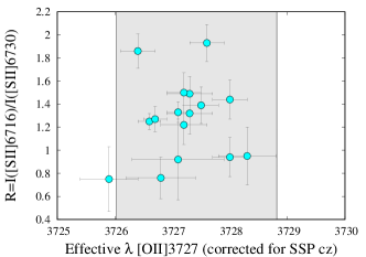
Figure 8: The intensity ratio [SII]$\lambda$6717/$\lambda$6731 as a function of effective wavelength of unresolved [OII]$\lambda\lambda$3726,3729 doublet corrected for SSP cz. Region inside the physical limits of the effective wavelengths of [Oii]$\lambda$3727 is shaded on the plot.

4.5 Relation between velocity dispersion of stellar and narrow-line components

There is considerable interest in the correlation of the supermassive black holes (SMBHs) masses $M_{\rm BH}$, with the stellar velocity dispersion of the host galaxy bulge (Gebhardt et al., 2000; Ferrarese & Merritt, 2000; Kormendy & Ho, 2013) because of its important implications to the coevolution of galaxies and their SMBHs. A problem affecting the definition of the $M_{\rm BH}$-$\sigma_{\star}$ relation for AGNs is that a strong optical continuum emission from the AGN accretion disk can make measuring $\sigma_{\star}$ difficult. Nelson & Whittle (1996) proposed using FWHM [Oiii]$\lambda$5007 as a proxy for $\sigma_{\star}\times\ 2.355$ because the [Oiii]$\lambda$5007 lines are strong and easily observable. The problem is that [Oiii]$\lambda\lambda$4959,5007  often display blue asymmetries, most often explained as an outflow component Heckman et al. (1981), that increase the scatter of the $M_{\rm BH}$– $\sigma_{\star}$ relation. Measuring of $\sigma_{\star}$ is more complicated in the case of AGN Type 1 because of the high influence of broad emission lines and strong featureless non-stellar continuum. Besides, just in several cases of recent studies (Du et al., 2016a; Sexton et al., 2019) $\sigma_{\mathrm{[OIII]}}$ and $\sigma_{\star}$ has been measured simultaneously. Sexton et al. (2019) showed that fitting the [Oiii]$\lambda$5007 line with a single Gaussian or Gauss-Hermite polynomials overestimates $\sigma_{\star}$ by more then 50%. Moreover, they showed that even when they exclude line asymmetries from non-gravitational gas motion in a fit with two Gaussians, there is no correlation between narrow component of $\sigma_{\mathrm{[OIII]}}$ and $\sigma_{\star}$. The fact that these two parameters have the same range, average and standard deviation implies that they are under the same gravitational potential (Sexton et al., 2019). They suggest that the large scatter is probably caused by dependency between the line profiles and the light distribution and underlying kinematic field. Because of this Sexton et al. (2019) strongly caution that the [OIII] width can not be used as a proxy for $\sigma_{\star}$ on an individual basis. This confirms the results of Bennert et al. (2018) who showed that $\sigma_{\mathrm{[OIII]}}$ can be used as a surrogate for $\sigma_{\star}$ only in statistical studies.
Komossa & Xu (2007) suggested to use [Sii]$\lambda\lambda$6731,6717 as a surrogate for $\sigma_{\star}$ since the sulfur lines have a lower ionization potential and do not suffer from significant asymmetries, but the scatter is comparable to that of the core of the [OIII] line.
In this work we confirm results of (Sexton et al., 2019) since we found no correlation between $\sigma_{\star}$ and the velocity dispersion of [Oiii]$\lambda$5007 narrow component. We instead found a high correlation between $\sigma_{\star}$ and the velocity dispersion of H$\beta$  narrow component ($r\approx$0.64, $P\approx 1.93E-05$). There is an overall consistency between the values of $\sigma_{\star}$ and both $\sigma_{\mathrm{[OIII]}}$ and $\sigma_{\mathrm{H\beta}}$: the median values of the ratios involving the three parameters and their semi inter-quartile ranges (SIQR) are: $<\sigma_{\mathrm{[OIII]}}$/$\sigma_{\star}>\approx 0.98\pm 0.23$, and $\sigma_{\mathrm{H\beta}}$/$\sigma_{\star}\approx 1.03\pm 0.19$, $\sigma_{\mathrm{[OIII]}}$/$\sigma_{\mathrm{H\beta}}\approx 0.93\pm 0.22$.

4.6 No strong outflows diagnosed by the [Oiii]$\lambda$5007 profile

As mention above [Oiii]$\lambda$5007 lines were fitted with two components - a narrower associated with the core of the line, and a semi-broad component that corresponds to the radial motions (e.g., Komossa et al., 2008; Zhang et al., 2011). The spectral range around [Oiii]$\lambda$5007 lines is zoomed on the middle plot of the figure 13. Figure 9 shows the distribution of the shift of the semi broad component in the HG sample. As for typical type 1 AGN, the distribution of the sources in our sample is skewed to the blue, especially toward the line base. The amplitude of the blue-shifts is however modest, and as so, not as strong as in the real xA sample. Looking at the full [Oiii]$\lambda\lambda$4959,5007 profiles we see again that no object qualifies as a blue outlier following the definition of (Zamanov et al., 2002), by far. The highest amplitude blueshift at 0.9 peak intensity is $\approx-150$  km s${}^{-1}\,$. The distribution of $c(\frac{1}{4})$ values is skewed toward blueshifts, as observed in most samples (e.g., Gaur et al., 2019; Berton et al., 2016; Zhang et al., 2011), in both Pop. A and Pop. B. The conclusion is that, for most objects, we have no evidence of xA properties from the [Oiii]$\lambda\lambda$4959,5007 profiles: large shifts are common among xA sources, with a high frequency of blue-outliers (Paper I).

4.6.1 The H$\beta$ broad profile

We expect a significant blueward asymmetry in the H$\beta$  broad profile of xA sources. If the profile is fit by a symmetric and unshifted Lorentzian function, a residual excess emission appears on the blue side of the Lorentzian profile (several examples are shown by Negrete et al. 2018). The blueshifted emission is associated with outflows that emit more prominently in high-ionization lines such as Civ$\lambda$1549Å  (see eg., Marziani et al., 2010, for a systematic comparison). Table 3 reports the centroid shifts of the H$\beta_{\rm BC}$  broad component. We see one clear example of blue shifted $c(\frac{1}{4})$ in the source SDSS J105530.40+132117.7, which has the highest $R_{\rm FeII}$ in our sample. Only this object appears to be a bona fide xA source. However, sources with $c(\frac{1}{4})$ $\lesssim-300$  km s${}^{-1}\,$  (assumed as a typical uncertainty at 1/4 maximum) are rare, just 6 out of 33. Most sources are symmetric or with the $c(\frac{1}{4})$ displaced to the red: more than one half (21/33) have a significant redward displacement. Prominent redward asymmetries are found among Pop. B sources, both radio quiet and radio-loud, with extreme cases in the radio-loud population (e.g., Punsly, 2013). The redward excess is associated with low Eddington ratio, although its origin is still not well-understood: tidally disrupted dusty clumps infalling toward the central black could be the cause of a net redshift (Wang et al., 2017), although other lines of evidence challenge this interpretation (e.g., Bon et al., 2015, and references therein).

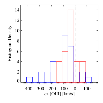
Figure 9: Left: Distribution of the shift of [OIII]$\lambda$5007 semi-broad component. Right: Distribution of the $c(\frac{1}{4})$ [Oiii]$\lambda$5007 (blue) and of the $c$(0.9) [Oiii]$\lambda$5007(red).

4.7 Properties of the host galaxy

In almost all objects we uncovered very high fraction of SSP spectra to the total flux (in the case of 17 objects even higher then 40%).

Restored mean stellar velocity (cz) is between -50  km s${}^{-1}\,$and 170  km s${}^{-1}\,$. Stellar velocity dispersion is between 90 km s${}^{-1}\,$and 220  km s${}^{-1}\,$. On the figure 14 we show $\chi^{2}$ maps in the space of SSP mean stellar velocity (cz) and SSP velocity dispersion. All SSP cz obtained from the single best fit are in a good agreement with values obtained from the $\chi^{2}$ maps, while SSP velocity dispersion obtained from the single fit are usually lower then those obtained from $\chi^{2}$ maps.
We found mostly old SSP (older then 1 Gyr). The metallicities of SSPs in our 32 sample are mainly Solar like. This property is at variance with the star formation property expected for xA sources. The UV spectral properties indicate extreme metal enrichment (Martínez-Aldama et al., 2018), most likely associated with extreme star formation detected in the FIR (Sani et al., 2010; Ganci et al., 2019, in the most luminous cases, SFR$\sim 10^{3}$ M_⊙ yr^-1.).

Table 5: Basic physical properties of the HG sample.

SDSS ID	$\log L_{5100}$	$\log M_{\mathrm{BH}}$	$\log\frac{L}{L_{\mathrm{Edd}}}$	$\log M_{\mathrm{BH}}\rm\ corr$	$\log\frac{L}{L_{\mathrm{Edd}}}\rm\ corr$
	[erg s-1]	[M⊙]		[M⊙]
J003657.17-100810.6	43.94	8.2	-1.42	8.1	-1.27
J010933.91+152559.0	43.73	8.2	-1.54	7.7	-1.07
J011807.98+150512.9	44.13	8.9	-1.92	8.5	-1.53
J031715.10-073822.3	44.08	8.8	-1.85	8.5	-1.50
J075059.82+352005.2	44.26	8.7	-1.56	8.3	-1.12
J082205.19+584058.3	44.07	8.8	-1.81	8.3	-1.36
J082205.24+455349.1	44.42	8.9	-1.57	8.2	-0.94
J091017.07+060238.6	44.08	8.6	-1.68	8.3	-1.36
J091020.11+312417.8	44.08	8.5	-1.51	8.5	-1.58
J092620.62+101734.8	43.83	8.2	-1.49	7.7	-0.97
J094249.40+593206.4	43.95	8.1	-1.22	7.3	-0.49
J094305.88+535048.4	44.05	8.9	-1.96	8.6	-1.62
J103021.24+170825.4	44.12	8.6	-1.58	8.1	-1.08
J105530.40+132117.7	44.19	8.4	-1.36	7.4	-0.35
J105705.40+580437.4	43.67	7.5	-0.95	7.5	-0.96
J112930.76+431017.3	43.65	8.2	-1.63	7.6	-1.02
J113630.11+621902.4	43.95	8.6	-1.73	8.0	-1.17
J113651.66+445016.4	43.51	8.1	-1.69	7.6	-1.21
J123431.08+515629.2	43.94	8.4	-1.56	7.9	-1.07
J124533.87+534838.3	44.14	8.6	-1.58	8.2	-1.16
J125219.55+182036.0	43.93	8.5	-1.65	7.9	-1.10
J133612.29+094746.8	43.88	8.3	-1.52	8.1	-1.37
J134748.06+404632.6	43.96	8.2	-1.33	8.0	-1.19
J134938.08+033543.8	43.84	8.0	-1.26	7.9	-1.16
J135008.55+233146.0	44.31	9.1	-1.88	8.5	-1.27
J141131.86+442001.0	43.91	8.4	-1.66	8.3	-1.47
J143651.50+343602.4	43.85	8.5	-1.79	8.3	-1.59
J151600.39+572415.7	43.82	8.0	-1.27	7.9	-1.18
J155950.79+512504.1	43.91	8.2	-1.42	7.8	-1.03
J161002.70+202108.5	43.82	8.1	-1.41	7.6	-0.90
J162612.16+143029.0	43.69	8.7	-2.09	8.4	-1.88
J170250.46+334409.6	43.90	8.3	-1.57	7.8	-1.01

5 Discussion

5.1 Interpretation in the Eigenvector 1 context

We notice consistent results between measurements of Shen & Ho (2014) and ours, albeit with a bias in favour of higher $R_{\rm FeII}$ for Shen & Ho (2014). According to the position of the spectra on the MS diagram of Fig. 1, objects are mainly Pop. B, with the exception of 5 sources that are of the Pop. A class. The distribution of the quasar data points is centered in Pop.B2, with 22 sources objects that belong or are likely to belong to Pop. B2, including borderline.

Apart from the location along the MS of Fig. 1, the conclusion that the wide majority of the HG sample sources are not xAs (only one source (J105530.40) meets in full the criterion of Negrete et al. (2018, $R_{\rm FeII}$$\gtrsim 1.2$) to qualify as an xA source) is reinforced by several lines of evidence: (a) [Oiii]$\lambda\lambda$4959,5007 profile without large blueshifts and [Oiii]$\lambda\lambda$4959,5007 consistent with the rest frame; (b) H$\beta_{\rm BC}$ profile symmetric or redward asymmetric; (c) HG component predominantly dominated by an old stellar population; (d) conventional estimates of the $L/L_{\rm Edd}$ $\ll$1. On this last line, we discuss in §5.2 a discrepancy between $L/L_{\rm Edd}$ estimates based on scaling laws and the new approach of the accreting black hole fundamental plane (Du et al., 2016a).

The previous analysis points toward a sample showing relatively low luminosity, and “milder” signs of nuclear activity with respect to the extreme radiators of xA. This does not mean that a similar phenomenology concerning nuclear outflows is not occurring, but its detectability is limited to some particular manifestations, such us the blueshift of [Oiii]$\lambda\lambda$4959,5007 close to the line base.

5.2 Basic physical properties

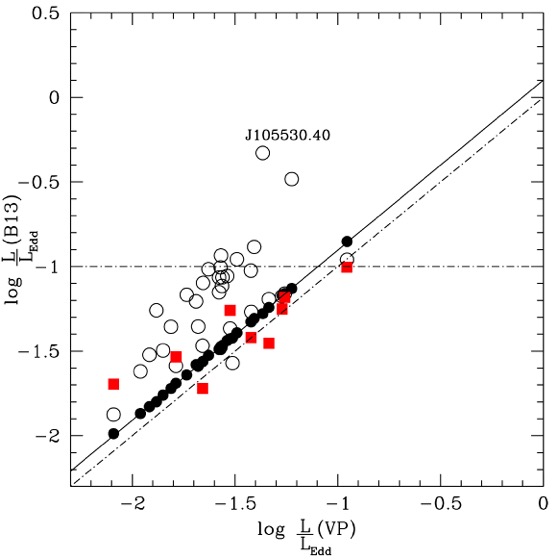
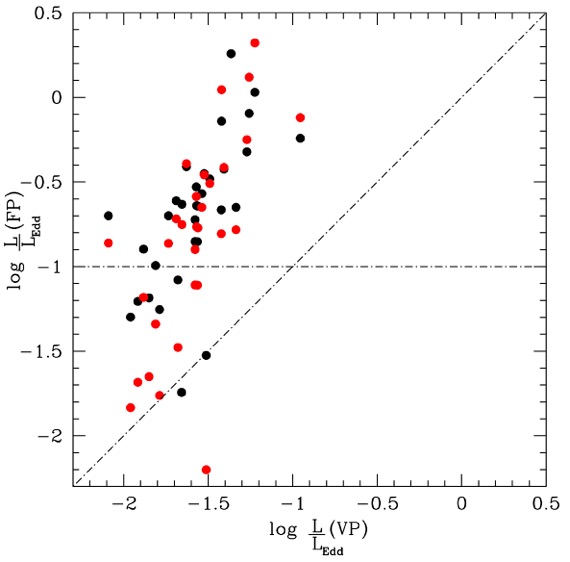
Figure 10: Left: relation between the Eddington ratio with $M_{\rm BH}$ computed from the scaling law of VP and with the $r_{\mathrm{BLR}}$ from Bentz et al. (2013) employing an uncorrected FWHM value (black circles). The open circles represents estimates using $f^{\star}_{2}$ (Eq. 4) and $r_{\mathrm{BLR}}$ corrected following Eq. 5. Red squares represents $L/L_{\rm Edd}$ estimates from the McConnell et al. (2011) scaling law, with the restriction of $\sigma_{\star}\gtrsim 150$ km s${}^{-1}\,$. The oblique dot-dashed line is the equality line; the horizontal one marks the conventional limit separating Pop. A and B. The filled line is the result of an unweighted lsq fit between the VP and the uncorrected Bentz et al. (2013) $M_{\rm BH}$ estimates. Right: relation between the Eddington ratio with $M_{\rm BH}$ computed from the scaling law of VP and the fundamental plane of Du et al. (2016b) (black circles), and after the re-fit of this paper (red circles).

Black hole masses estimates using scaling laws for large samples of AGN are subject to a large uncertainty, due to both systematic and random errors (exhaustive reviews are given in Marziani & Sulentic, 2012; Shen, 2013). However, in the case of the low-$z$ sample of the present work, we can count on the H$\beta$  line width that is considered a reliable “virial broadening estimator” (Trakhtenbrot & Netzer, 2012, with the caveats of Marziani et al. 2013a, 2019). Table 5 lists basic physical properties of the AGN - the log of the 5100 $\AA$ AGN luminosity scaled by the AGN power-law continuum fraction to the total flux, the black hole mass $M_{\rm BH}$ computed following the prescription of Vestergaard & Peterson (2006, hereafter, VP), and $L/L_{\rm Edd}$ (assuming the bolometric luminosity to be 10 times the luminosity at 5100 Å; Richards et al. 2006). In this table we present also the corrected $M_{\rm BH}$and $L/L_{\rm Edd}$ according to the prescription of Martínez-Aldama et al. (2019) (see 5.3). The $M_{\rm BH}$ values following VP indicate a population of quasars of relatively modest $M_{\rm BH}$, $\sim 10^{8}$ M_⊙. Accepted at a face value, $L/L_{\rm Edd}$ is typical of Pop. B, with some objects close to the boundary between A and B but formally on the side of Pop. B, if $L/L_{\rm Edd}$$\approx 0.1-0.2$ is assumed as the $L/L_{\rm Edd}$ threshold for Pop. A sources.

We can write the expression of the virial mass as follows:

$$M_{\mathrm{BH}}=f\frac{r_{\mathrm{BLR}}(\delta v)^{2}}{G}=f_{1}(\dot{m},a)f_{2}(\theta\,|\,\dot{m})\frac{r_{\mathrm{BLR}}(\delta v)^{2}}{G},$$ (2)

where $r_{\mathrm{BLR}}$ is the BLR radius, $a$ is the spin parameter of a black hole, and we considered as estimator of the virial broadening velocity spread $\delta v=$FWHM, the FWHM of the broad component of H$\beta$ . We have written the structure or form factor $f$ as the product of two terms, one depending on accretion rate and black hole spin, and one depending on orientation. The dependence of $f_{1}$ on dimensionless accretion rate has been emphasized by the $r_{\mathrm{BLR}}$ dependence on luminosity (Du et al., 2016a) which, for xA sources, is not consistent with the general AGN population. The dependence of $f_{1}$ on the spin parameter is unknown, but is expected since the spin in influencing the temperature of the accretion disk and hence the SED of the ionizing continuum (e.g., Wang et al., 2014b). To complicate the issue, the orientation effects are also expected to be dependent on $\dot{m}$ (Wang et al., 2014c), as a geometrically thin optically thick disk may be considered as a Lambertian radiator (with some limb-darkening effects at high inclination Netzer 2013), but free of the self-shadowing effects expected for a geometrically thick disk. Keeping for the moment with the simplest approach, we can compute the $M_{\rm BH}$ by using the Bentz et al. (2013, hereafter, B13) correlation between $r_{\mathrm{BLR}}$ and optical luminosity, assuming $f=1$. The results are tightly correlated with the mass estimate obtained from the VP relation (Fig. 10). The extremely tight correlation is expected as the VP assumes the same virial relation and only a slightly different value of the zero point and of the $r_{\mathrm{BLR}}$ - $L$ correlation. The small bias between the two relations is understood in terms of a constant difference in the $f$ factor, since VP assumed $f=0.75$. In both cases no orientation effects are considered. Typical uncertainties in the $M_{\rm BH}$ are expected to be $\approx 0.3$ dex at 1 $\sigma$ (Vestergaard & Peterson, 2006; Marziani et al., 2019), most likely because of differences in $f$  associated with different structure ($f\lesssim$ 1 and $\approx 2$ were derived for Pop. B and A, respectively Collin et al., 2006), and with the effect of orientation. The $r_{\mathrm{BLR}}$ - $L$ is also known to be dependent on $\dot{m}$ (Du & Wang, 2019, and references therein). The main source of uncertainty in luminosity estimates at 5100 Å is the continuum placement and the error associated with the decomposition of between the AGN and host continua. Even if formal errors are low, it is unlikely that the uncertainty is less than $\approx$ 10%, which we assume as an indicative value. The computation of the bolometric luminosity suffers from the additional scatter associated with the diversity in the AGN SEDs; scatter at 1$\sigma$ could be assumed $\sim$ 20% (Elvis et al., 1994; Richards et al., 2006). We expect a dependence of the bolometric correction along the main sequence; more recent estimates suggest a dependence on luminosity, spin and dimensionless accretion rate (e.g., Runnoe et al., 2013; Netzer, 2019), but they are relatively untested and were sparsely considered in past work. We assume bolometric correction 10.

5.2.1 $L/L_{\rm Edd}$ estimate using the Fundamental Plane

A second method to estimate $L/L_{\rm Edd}$ can be based on the fundamental plane (FP) of accreting black holes described by Du et al. (2016b). Du et al. (2016b) introduced the notion of the fundamental plane of SEAMBHs defined by a bivariate correlation between the parameter $\dot{{\mathcal{M}}}=\frac{\dot{M_{\rm BH}}c^{2}}{L_{\mathrm{Edd}}}$ i.e., the dimensionless accretion rate $\dot{m}=\frac{\eta\dot{M}c^{2}}{L_{\mathrm{Edd}}}$  for $\eta=1$ (Du et al., 2015), the Eddington ratio, and the observational parameters $R_{\rm FeII}$ and D parameter (ratio $FWHM/\sigma$ of H$\beta$, where $\sigma$ is the velocity dispersion of the broad component of H$\beta$ ). The FP can then be written as two linear relations between $\log\dot{\cal M}$ and $L_{\rm L}/L_{\rm Edd}$ versus $\approx a+b\frac{\rm FWHM}{\sigma}+cR_{\rm FeII},$ where $a,b,c$ are reported by Du et al. (2016b). The identification criteria included in the fundamental plane are consistent with the ones derived from the E1 approach ($L/L_{\rm Edd}$ and $\dot{{\mathcal{M}}}$ increase as the profiles become Lorentzian-like, and $R_{\rm FeII}$ becomes higher).

To investigate the origin of this disagreement, we considered that the fit provided by Du et al. (2016b) is very good for high Eddington radiators but is biased if low $L/L_{\rm Edd}$ data are considered. The upper panel of Fig. 11 shows that there is a significant residual between data and fit values that is dependent on $L/L_{\rm Edd}$: at low Eddington ratio, $\log$ $L/L_{\rm Edd}$ $\sim-2$, the FP plane fit reported by Du et al. (2016b) predicts a value of $L/L_{\rm Edd}$ almost one order of magnitude systematically higher with respect to the one inferred by the distribution of the data points. The residuals can be fit by a linear function ($\delta=\log$$L/L_{\rm Edd}$$-\log$$L/L_{\rm Edd}$(FP) that zeroes the trend in Fig. 11 (red dots), with a post-correction best fitting line consistent with $\delta$($L/L_{\rm Edd}$) $\equiv 0$. Applying the correction to the residuals to obtain new values of $L/L_{\rm Edd}$ we obtain this slightly modified equation for the fundamental plane $\log$ $L/L_{\rm Edd}$= $\alpha+\beta D+\gamma$$R_{\rm FeII}$$\approx 0.774-1.33D+1.30$$R_{\rm FeII}$. The estimates with this new law, although lower at the low $L/L_{\rm Edd}$ do not solve the disagreement between the VP conventional estimates and the FP estimates (Fig 10). The right panel of Fig. 10 shows that the FP $L/L_{\rm Edd}$ estimates are in large disagreement with respect to the VP and B13 estimates with both the old and new equation for FP : VP estimates are below by more than one order of magnitude the ones based on the FP. The disagreement is so serious that the highest radiating source with $L/L_{\rm Edd}$$\sim$ 2 according to the FP has $L/L_{\rm Edd}$$\approx 0.04$ following VP, and that it leads to inconsistencies between the MS interpretation and spectral type assignment: the same source would qualify as a Pop. B source (VP) and as an xA (FP). Using the modified VP with the parameters reported above, the only effect is to bring in agreement only 6-7 points at the low-$L/L_{\rm Edd}$ end. The bulk of the data point remains above the VP estimates by $\approx$1 dex.

To further investigate the issue, we computed $M_{\rm BH}$  from the stellar velocity dispersion $\sigma_{\star}$ of the host bulge, using the scaling law $M_{\rm BH}$ $\approx 1.95\cdot 10^{8}\left(\sigma_{\star}/200\right)^{5.12}$ M_⊙ (McConnell et al., 2011), which is an updated formulation of the original scaling law of Ferrarese & Merritt (2000). Fig. 12 shows that the VP $M_{\rm BH}$  and $M_{\rm BH}$ from host show systematic differences that are strongly correlated with $\sigma_{\star}$, increasing with decreasing $\sigma_{\star}$. The unweighted least squares fitting line shown in Fig. 12 represent a highly significant but likely spurious correlation. When physical velocity dispersion is of the same order or smaller than the instrumental velocity dispersion, it is advisable Koleva et al. (2009a) to inject line spread function (LSF) of the spectrograph in the model of SSP, in order to adjust the resolution of the spectra and the model. We re-fitted the spectra where $\sigma_{\star}$ was below 150  km s${}^{-1}\,$, with injected LSF in the SSP model, but restored $\sigma_{\star}$ was just slightly higher then the first estimation of $\sigma_{\star}$, and still within the error bars of the first estimation. Therefore, we concluded that LSF injection would not solve the problem of discrepancies between two estimations of the masses. There is a possibility, discussed in § 5.3 that $\sigma_{\star}$ is associated with systems observed face-on, and that are therefore also affected by orientation effects.

The FP estimates are based on two parameters that do not include information on line broadening. The parameter $D$ is somewhat redundant as the shape of the H$\beta$  profile is known to be a MS correlate: the profiles are Gaussian-like ($D\approx 2.3$) in Population B, while become Lorentzian-like in Pop. A (spectral type 1) and are consistent with Lorentzian-like up to the highest $R_{\rm FeII}$ value, albeit with a blueshifted excess interpreted as Balmer emission from a high-ionization wind, more easily detected in high-ionisation lines such as Civ$\lambda$1549Å  (e.g., Richards et al., 2011). Therefore the behaviour of the parameter D is not expected to be monotonic along the sequence: it should increase from extreme Pop. B toward A1, where the most Lorentzian-like profiles are observed, and decrease again where a blueshift excess provides a significant deviation from a Lorentzian profile (ST A3 and A4). In addition, what would be the prediction passing from A2 to B2 and from A3 to B3 according to the fundamental plane? The xA sources of A3 in the sample of Du et al. (2016a) show a typical $D\approx 1.5$; in B3 the profiles are more Gaussian-like, and we can assume a conservative $D\approx 2$; for the same average $R_{\rm FeII}$= 1.25, the change in $L/L_{\rm Edd}$ would be more than a factor $2.5$. These consideration focus the issue on the nature of Pop. B2 and B3. Populations B2 and B3 are rare at low $z$ (B2 are $\lesssim$3% in the sample of Marziani et al. 2013a; B3 is not even detected, which implies a prevalence $\lesssim 0.2$%), and represent a poorly understood classes. There is a degeneracy between effects of orientation and $M_{\rm BH}$ in the optical plane of the MS; for a fixed $M_{\rm BH}$, A2 sources seen at higher inclination may be displaced into B2 (Panda et al., 2019). At the same time we cannot exclude that higher $M_{\rm BH}$ sources are located within B2. In both cases, for a fixed luminosity, we expect a significant decrease in $L/L_{\rm Edd}$ passing from B2 to A2.

Besides, the object could appear as B2 type, due to different response of H$\beta$ and Feii flux to the variability of ionizing continuum. Higher $R_{\rm FeII}$  could be caused by two variability effects: (1) a faster response of H$\beta$ flux to the variability of ionizing continuum; (2) a larger amplitude of H$\beta$ flux variations compared to the amplitude of Feii flux variations (see e.g. Hu et al., 2015; Barth et al., 2013). In case of observing single epoch spectra, depending on variability state both effects, together with the line width response to the flux variations, could contribute to estimates of mass and $L/L_{\rm Edd}$ . Also, these effects could produce the trend of $L/L_{\rm Edd}$  decreasing with $R_{\rm FeII}$ (Bon et al., 2018), which is opposite to the trend along EV1 where $L/L_{\rm Edd}$  increase with $R_{\rm FeII}$ (Marziani et al., 2013b).

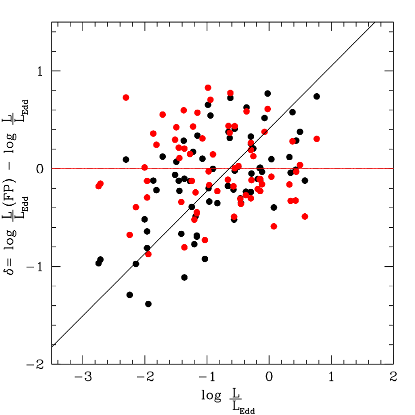
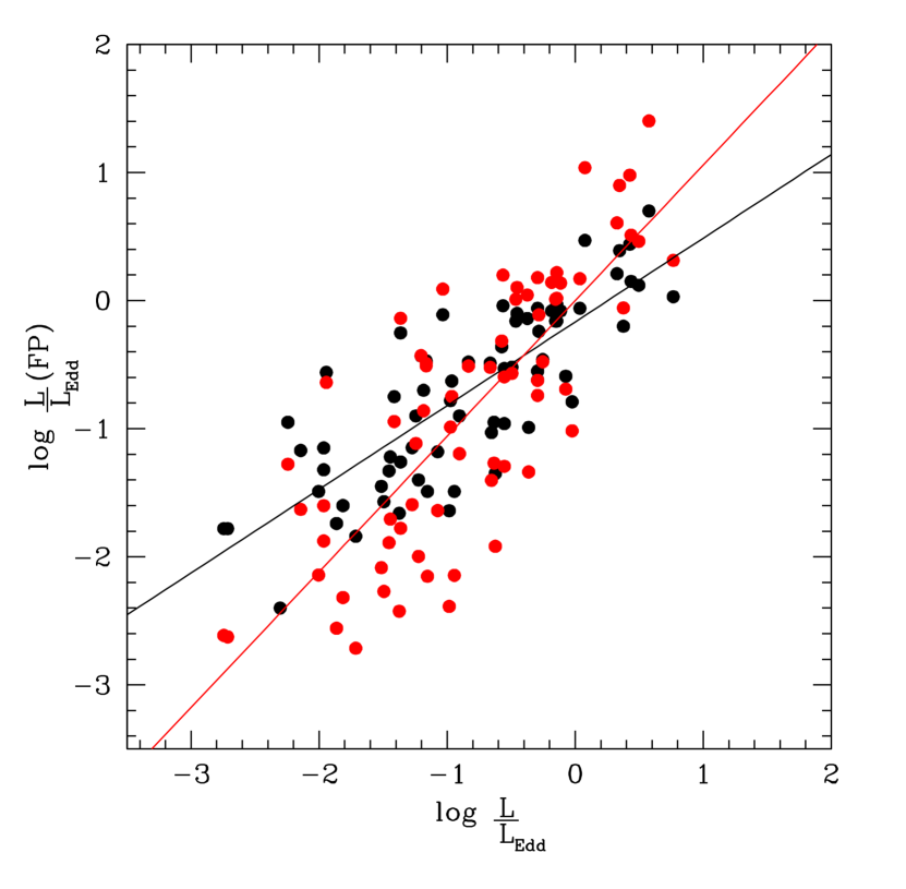
Figure 11: Improvement on the fundamental plane of accreting black holes. Top panel shows residuals between the original FP fitting equation of Du et al. (2016b) and the data (black circles). There is a significant linear trend; the black line traces the unweighted lsq best fit. The red circles show the residuals with the modified FP (see § 5.2.1); there is no trend, and the best fitting (red) line is consistent with zero slope (black line). The bottom panel shows the data points with $L/L_{\rm Edd}$ estimated with the original (black) and revised (red) FP equation.

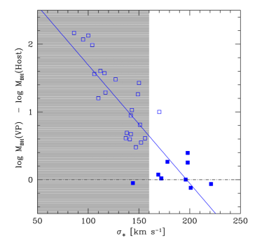
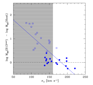
Figure 12: Top: Relation between velocity dispersion $\sigma_{\star}$ and difference between $M_{\rm BH}$ estimates from $\sigma_{\star}$ using the scaling law of McConnell et al. (2011) and the scaling law from VP. The shaded area identifies the range of $\sigma_{\star}\leq 160$  km s${}^{-1}\,$. All data point save one with McConnell et al. (2011) $M_{\rm BH}$ values yielding large systematic differences ($>$ 0.4, represented with open squares) with respect to the VP $M_{\rm BH}$  are within the shaded area. Bottom: same as in the top panel but with the $M_{\rm BH}$ values computed with the correction described in §5.3.

5.3 Orientation and physical parameter estimates

The previous analysis ignored the effect of orientation on the $M_{\rm BH}$ computation. However, growing evidence suggests that the low-ionization lines-emitting BLR is highly flattened (e.g., Mejía-Restrepo et al., 2018, and references therein). If this is the case, the observed velocity can be parameterized as $\delta v^{2}_{\mathrm{obs}}=\delta v_{\mathrm{iso}}^{2}/3+v_{\mathrm{Kepl}}^{2}\sin^{2}\theta$, and if $\delta v_{\mathrm{iso}}/\delta v_{\mathrm{Kepl}}\approx 0.1$, where $\delta v_{\mathrm{iso}}$ is an isotropic velocity component, and $\delta v_{\mathrm{Kepl}}$ the Keplerian velocity. For a geometrically thin disk, it implies $\delta v_{\mathrm{obs}}\approx\delta v_{\mathrm{Kepl}}/\sin\theta$ (if the FWHM is taken as the $\delta v_{\rm obs}$, and $\delta v_{\rm Kepl}=0$ i.e., in the case of isotropic velocity dispersion, $f_{2}=\frac{3}{4}$). If the VBE estimates are not corrected beforehand for orientation, the structure (or form) factor is $f_{2}\propto 1/\sin^{2}\theta$ (e.g., McLure & Dunlop, 2001; Jarvis & McLure, 2006; Decarli et al., 2011), and more precisely (we assume $f_{1}\equiv 1$):

$$f_{\rm 2}=\frac{1}{4\left[\frac{1}{3}\left(\frac{\delta v_{\rm iso}}{\delta v_{\rm K}}\right)^{2}+\sin^{2}\theta\right]}.$$ (3)

We attempt to consider the effect of the viewing angle on the H$\beta$  line width by considering that the virial factor is anti-correlated with the FWHM of broad emission line. For the H$\beta$  line the relation is given by

$$f_{2}^{\star}=\left(\frac{{\mathrm{FWHM}}}{4550}\right)^{-1.17},$$ (4)

(Mejía-Restrepo et al., 2018). This implies that sources with FWHM H$\beta$  narrower than $4550$ km s${}^{-1}\,$ should have their mass increased by a factor that can be as large as $\approx 5$ in the case of the narrowest H$\beta$  profiles observed in NLSy1s. The effect is milder than the one predicted by Eq. 3, and may be better suited for the general population of quasars encompassing both typical Pop. A and B sources. In addition, Martínez-Aldama et al. (2019) suggested a correction to the B13 $r_{\mathrm{BLR}}$ estimate, following the reverberation mapping campaign of highly accreting quasars (Du et al., 2018, and references therein), $\delta r_{\mathrm{BLR}}=\mathrm{log}\,\left({r_{\mathrm{BLR}}}/{r_{\mathrm{{BLR,B13}}}}\right)$. According to Martínez-Aldama et al. (2019), with the $f^{\star}_{2}$ dependence on FWHM, the correction to $r_{\mathrm{BLR}}$  is:

$$\delta r_{\mathrm{BLR}}=\left(-0.271\pm 0.030\right)\mathrm{log}\,\frac{L\mathrm{{}_{bol}}}{L\mathrm{{}_{Edd}}^{\star}}\,+\left(-0.396\pm 0.032\right),$$ (5)

where ${L\mathrm{{}_{Edd}}^{\star}}$ means that the Eddington luminosity has been computed with virial mass relation assuming $f^{\star}_{2}$ (Eq. 4). The $L/L_{\rm Edd}$ values computed with this approach deviate significantly from the VP and B13 $L/L_{\rm Edd}$, yielding a higher value of $L/L_{\rm Edd}$ (Fig. 10), because most of the sources have FWHM H$\beta$ $\gtrsim 4500$, and hence $f^{\star}<1$ which implies a lower $M_{\rm BH}$. The effect visible in Fig. 10 comes mostly from the $f^{\star}_{2}$: the $\delta r_{\mathrm{BLR}}$ is small since $L/L_{\rm Edd}$ is low ($\log$ $L/L_{\rm Edd}$$\sim-1.-1.5$). The agreement between the modified VP and the FP remains poor. After the corrections, however, the xA candidate SDSSJ105530.40+132117.7 is recognised as the highest radiator, with $L/L_{\rm Edd}$ $\approx-0.35$, close to the conventional lower limit for xA sources. We can conclude that the objects in our sample are safely not xA (apart from the one source mentioned right above, and perhaps a couple of borderline cases). Are they of Pop. A? Following the FP all save 7 should be of Pop. A, with 5 xA candidates (Fig. 10). Following the modified expression of Eq. 4, about one half of the sources has $\log$ $L/L_{\rm Edd}$$\gtrsim-1$, the conventional boundary between Pop. A and B.

If we consider the modified viral mass as described in the previous paragraph, any correlation with the McConnell et al. (2011) remains fairly weak ($r\approx 0.385$, significant at just $2\sigma$ confidence level). However, the bottom panel of Fig. 12 shows that now more than half of the sample has masses in reasonable agreement with ones from the host. For the remaining sources with small $\sigma_{\star}$, we consider that bulges seen face-on should be considerably affected by orientation in their measured velocity dispersion, as they are rotationally supported (Kormendy & Illingworth, 1982). A test of this possibility goes beyond the goals of the present paper.

The existence of a relation between $R_{\rm FeII}$ and $L/L_{\rm Edd}$  is a robust result and rests on several lines of evidence (Grupe et al. 1999; Kuraszkiewicz et al. 2004; Dong et al. 2011; Marziani et al. 2013b; Sun & Shen 2015, in addition to the analysis of Du et al. (2016a); Du & Wang (2019)). For instance Marziani et al. (2013b) showed (their Fig. 6) that there is a $L/L_{\rm Edd}$ systemic trend along Pop. A, with $L/L_{\rm Edd}$ increasing with $R_{\rm FeII}$. Independent evidence is provided by Sun & Shen (2015): for the luminosity in a fixed range, the $\sigma_{\star}$ (a proxy of $M_{\rm BH}$) decreases systematically with increasing $R_{\rm FeII}$ up to $R_{\rm FeII}$$\sim 1$. Indirect evidence is also provided by one of the correlations of 4DE1: the highest correlation coefficient is between $R_{\rm FeII}$ and Civ$\lambda$1549Å  blueshift amplitude (Sulentic et al., 2000c, 2007, 2017). The balance between radiative and gravitational forces is able to account for a large part of the quasars optical/UV phenomenology along the quasar MS (Ferland et al., 2009). Therefore the key factor in the discrepancy of the $L/L_{\rm Edd}$ estimates around A2/B2 is most likely to be orientation, as the viewing angle $\theta$ affects FWHM H$\beta$  linearly, and $M_{\rm BH}$ quadratically. By the same token a large fraction of the B2 sources could be very well intrinsically Pop. A, especially the ones with $R_{\rm FeII}$ significantly above 0.5 and FWHM borderline.

Great care should be used in the computation of the $M_{\rm BH}$ and $L/L_{\rm Edd}$ if no orientation correction is possible. As a test not related to the present sample, we considered the sources of the Du et al. (2016a) sample that are xA i.e., satisfying the criterion $R_{\rm FeII}$$>1.2$ following Negrete et al. (2018). For these 6 sources the $L/L_{\rm Edd}$ average value applying the original FP is $\approx 0.45$, implying that they should be considered true “super-Eddington” accreting massive black holes (SEAMBHs Wang et al., 2014a). For these xA sources, it is possible to derive an estimate of the viewing angle $\theta$ (Negrete et al., 2018): the difference between the virial luminosity estimate and the concordance luminosity (assumed to be the correct luminosity) is expected to be mainly dependent on the viewing angle, which is assumed to strongly affect the FWHM according to Eq. 3. For these sources, $\theta\sim$0.2 rad: their emitting regions are expected to be seen almost face-on. If the $M_{\rm BH}$ are recalculated following Eq. 2 and Eq. 3 with the $\theta$ estimated following Negrete et al. (2018), the $L/L_{\rm Edd}$ is lowered to an average $\approx-0.147$, consistent with the estimates using the conventional approach (Marziani & Sulentic, 2014). The Negrete et al. (2018) approach can not be extended to the sample of the present paper, but it is a strong indication that $L/L_{\rm Edd}$ actual values depend on a normalization factor that is in turn dependent on the viewing angle, via the dependence on the viewing angle of $M_{\rm BH}$. The xA sources apparently radiate at a limiting Eddington ratio along the MS. However, it is unclear whether the xA sources are truly SEAMBHs. Even if there is a consistency in the selection criteria, their Eddington ratios and $\dot{{\mathcal{M}}}$ are too much affected by uncertainties in the $M_{\rm BH}$ to be a safe discriminant.

6 Conclusions

This paper has analysed a spin-off of the Negrete et al. (2018) sample, and precisely spectra that were preliminary selected as xA candidates and afterwards found to suffer strong contamination by the spectrum of the host galaxy. Main results encompass

1. A proper identification of xA sources requires a careful simultaneous multicomponent fit in order to retrieve information on the stellar continuum and on the FeII emission, especially if the AGN is of low luminosity, and the data are from optical fiber with a relatively large angular coverage. Inclusion of the spurious xA sources should be avoided, as in cosmological studies it may dramatically increase the dispersion in the Hubble diagram of quasars obtained from virial luminosity estimates.

2. Objects of our sample with strong host galaxy contamination show properties that suggest more modest activity, in comparison to xA sources. Modest activity means that they lack extreme outflows, strong starburst activity, and high accretion rate, typical of xA sources.

3. We found a high fraction of host galaxy spectrum (in half of the sample even higher then 40%). We conclude that when absorption lines are prominent, and the fraction of the host galaxy is high, SSP is mimicking FeII, and that this can lead to mistaken identification of FeII spectral features. We have identified several stellar absorption lines that, along with the continuum shape, may lead to an overestimate of $R_{\rm FeII}$, and therefore to the misclassification of sources as xA sources. Our results lead support to the results of Śniegowska et al. (2018) who found that only six sources out of a sample of 23 could be classified as xA after a careful decomposition of all spectral components involving also the spectrum of the host galaxy.

4. We have studied the 32 sources with high host galaxy contamination as an independent sample which has an interest of its own. We have used a host galaxy shift as a reference frame in order to study shifts of emission lines more precisely. Unlike xA sources, there is a very good agreement between the shift of absorption spectrum and the shifts of H$\beta_{\rm NC}$, [Oii]$\lambda$3727, and the [Oiii]$\lambda$5007. The good agreement between [Oiii]$\lambda$5007 and the narrow low-ionisation lines H$\beta_{\rm NC}$ and [Oii]$\lambda$3727 has important consequences for the systemic redshift estimates in case no host absorptions could be detected.

5. We have considered the effect of the density on the effective wavelength of the [Oii]$\lambda$3727 doublet, providing a relation linking $n_{\mathrm{H}}$ and $\lambda_{eff}$. The dependence on density introduces a significant error in [Oii]$\lambda$3727-based redshift estimates. However, the effective wavelength density dependence could be in principle provide a diagnostics of the relative importance of the AGN NLR and of circum-nuclear star formation producing low-density Hii regions.

6. We found mostly old SSP (older then 1 Gyr) for the HG. The metallicities of SSPs in our 32 sample are mainly solar.

7. The HG sources cluster around spectral type B2. Considering the spectral type correlation with $L/L_{\rm Edd}$, a large fraction of them should be considered inclined Pop. A sources.

8. Computations of $M_{\rm BH}$ are problematic, especially if small samples of heterogeneous sources involving a broad range of H$\beta$  FWHM are considered (see e.g., Shen, 2013). We have discussed estimates of $M_{\rm BH}$ and $L/L_{\rm Edd}$, and emphasized the effect of orientation that should be considered if a meaningful comparison of $L/L_{\rm Edd}$ values between sources of widely different width has to be done. In principle, if viewing angles were known for each source, the $M_{\rm BH}$ and $L/L_{\rm Edd}$ values could be normalised to a standard $\theta$, to let physical trends emerge more clearly. Individual $\theta$ estimates are still unavailable for the general population of quasars outside of the MS extremes such as the ones considered in this study, although $\theta$ computations may become widespread in the coming years. Spectropolarimetric measurements, even if demanding in terms of telescope time, have provided individual $\theta$ values for sources in different spectral types along the MS (Afanasiev & Popović, 2015). Other techniques, based on the SED also show promising possibilities (Capellupo et al., 2015; Mejía-Restrepo et al., 2018).

9. At this point, one has to consider that the VP scaling law, perfectly consistent with the use of the more recent Bentz et al. (2013) $r_{\mathrm{BLR}}$ scaling law is biased in favor of broader sources (i.e., the many Population B sources that were targets of early reverberation mapping campaigns). On the converse, the $L/L_{\rm Edd}$ estimates from the Du et al. (2016b) fundamental planes are apparently biased toward narrow sources (i.e., the many NLSy1s and Population A sources that are included in the Du et al. 2016b sample). In both cases, a small FWHM is taken as a synonym of small $M_{\rm BH}$, and a broad FWHM as synonym of large $M_{\rm BH}$. Presently, we know this is not the case because of the degeneration between mass and orientation effects. The present work let emerge how VP overestimate the $M_{\rm BH}$ and underestimate $L/L_{\rm Edd}$, and how Du et al. (2016b) underestimate the $M_{\rm BH}$, and overestimate $L/L_{\rm Edd}$. These problems are likely to be overcome by the next-generation SDSS-V panoptic spectroscopy (Kollmeier et al., 2017), multi-epoch spectroscopic survey of over six million objects that plans reverberation-mapping quality monitoring for thousands of quasars.

Appendix A SSP analysis atlas

Fig. 13 shows the appearance of the spectrum in the range 4000 – 5500 Å where the fit was carried out, a zoom around H$\beta$  and [Oiii]$\lambda\lambda$4959,5007, and the cleaned H$\beta$  profile for the sources of the HG sample. The follow-up measurements of the individual spectra obtained after the fitting with ULySS are reported in Table 2. Although in the case of few spectra the narrow and semi-broad component of [Oiii]$\lambda$5007 lines have switched places, we carefully disentangle the two components according to their widths.

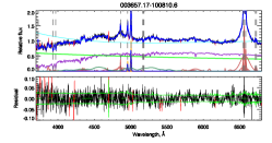
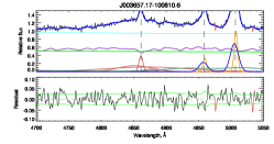
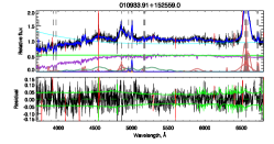
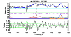
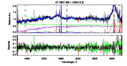
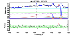
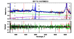
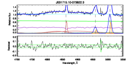
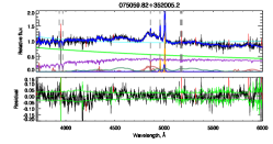
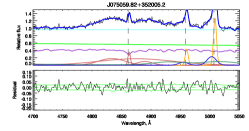
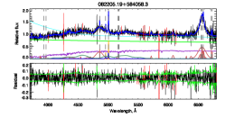
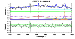
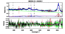
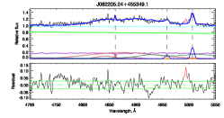
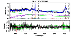
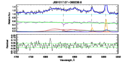
Figure 13: Ulyss fits to the HG sample. In the upper left panel, the black line represents the observed spectrum, the blue one the best fit, the red line the multiplicative polynomial, while the green, light red, and violet lines represent components of the best fit: violet – stellar population, red – emission lines, and green – AGN continuum. The bottom left panel shows the residuals of the best fit (black line). The green solid line shows the level of the noise, and the dashed line is the zero-axis. Middle panels zoom the domain around H$\beta$ and [Oiii]$\lambda$5007 lines, while right hand panels show the model broad H$\beta$.

*

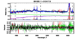
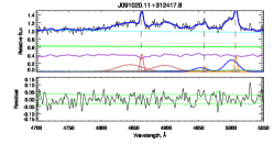
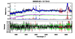
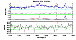
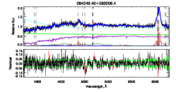
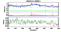
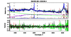
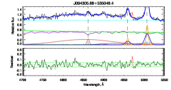
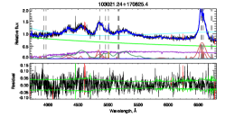
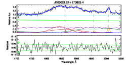
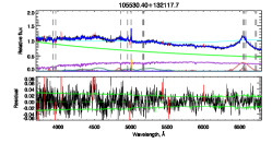
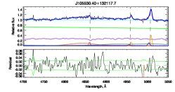
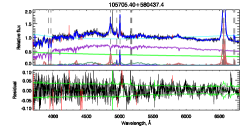
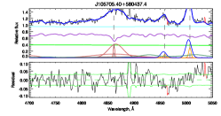
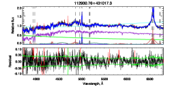
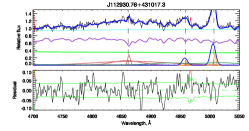
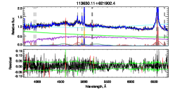
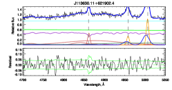
Figure 13: – continued

*

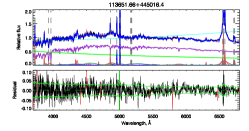
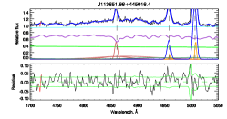
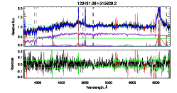
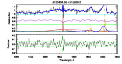
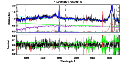
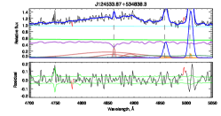
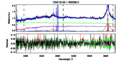
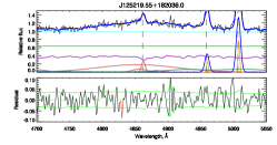
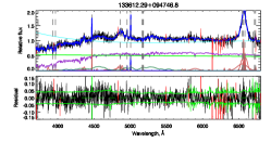
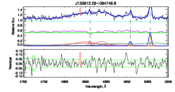
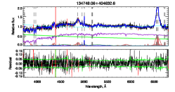
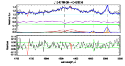
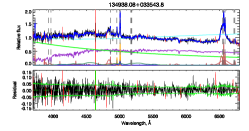
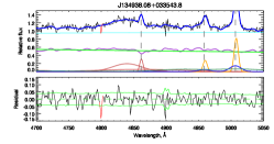
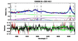
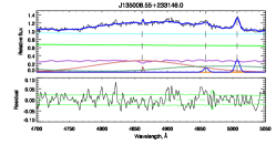
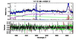
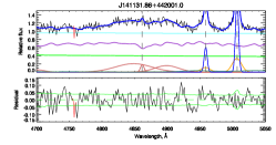
Figure 13: – continued

*

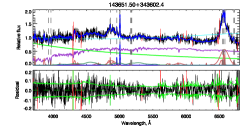
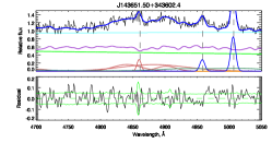
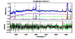
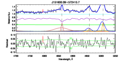
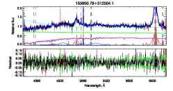
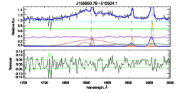
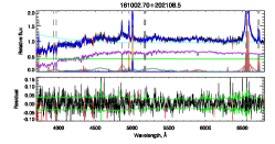
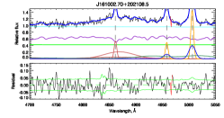
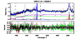
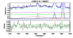
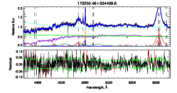
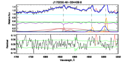
Figure 13: – continued

Figure 14 represents the $\chi^{2}$ maps for the whole sample in the parameter space of the stellar velocity dispersion and the mean stellar velocity.

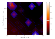
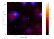
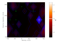
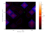
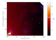
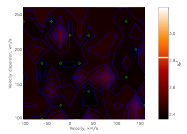
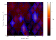
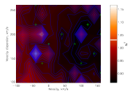
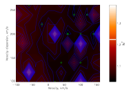
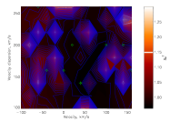
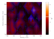
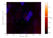
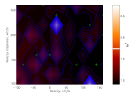
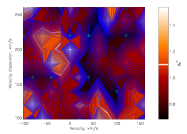
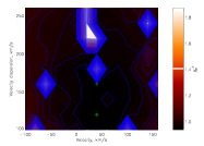
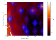
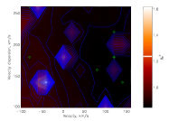
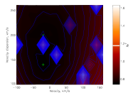
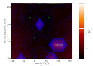
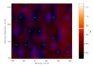
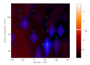
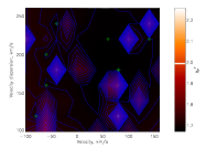
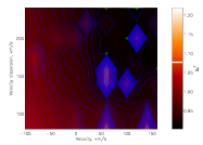
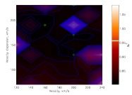
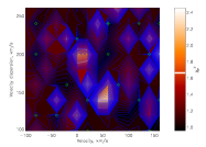
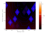
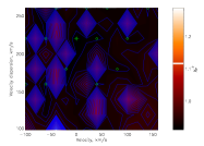
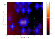
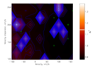
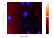
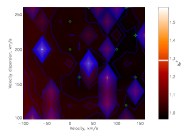
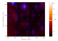
Figure 14: $\chi^{2}$ maps in the space of SSP mean stellar velocity and SSP velocity dispersion. Color-bar on the right hand side of $\chi^{2}$ maps show $\chi^{2}$ value normalized for the signal-to-noise value of the spectrum, measured by the SDSS in the $g$-band.

Appendix B A method to derive emissivity weighted $n_{e}$ from $\lambda_{\mathrm{eff}}$ of [Oii]$\lambda$3727

Figure 15 shows the behavior of $\mathcal{R}$=$I$([Oii]$\lambda$3729)/$I($[Oii]$\lambda$3726) as a function of [Oii]$\lambda\lambda$3726,3729 doublet effective wavelength ($\lambda_{\mathrm{eff}}$) for an unresolved mock doublet of 4 and 5 Å. The $\lambda_{\mathrm{eff}}$ has been measured for mock profiles built for 11 values of $R$ with a step $\delta\mathcal{R}=0.1$. A cubic or quadratic fit reproduces the value of $R$:

$$\mathcal{R}(n_{\mathrm{e}})=k_{3}(\lambda_{\mathrm{eff}}-3727)^{3}+k_{2}(\lambda_{\mathrm{eff}}-3727)^{2}+k_{1}(\lambda_{\mathrm{eff}}-3727)+k_{0}$$ (6)

with the coefficients given in Table 6. The three width cases suggest a monotonic behavior of $\mathcal{R}$ as a function of $\lambda_{\mathrm{eff}}$, with $\lambda_{\mathrm{eff}}$ changing by $1.5$Å from 3727.5 Å and 3729.0 Å. The measurements carried out from half peak intensity (filled circles in Fig. 15) are more sensitive to the centroid differences and should be preferred in practice to fits from the base of the line.

The best-fit parameters of $\mathcal{R}$ as a function of $n_{\mathrm{e}}$ using up-to-date atomic data are shown in Table 7 for [Oii] from Sanders et al. (2016). Coefficients refer to a function of the form

$$\mathcal{R}(n_{\mathrm{e}})=a\frac{b+n_{\mathrm{e}}}{c+n_{\mathrm{e}}}.$$ (7)

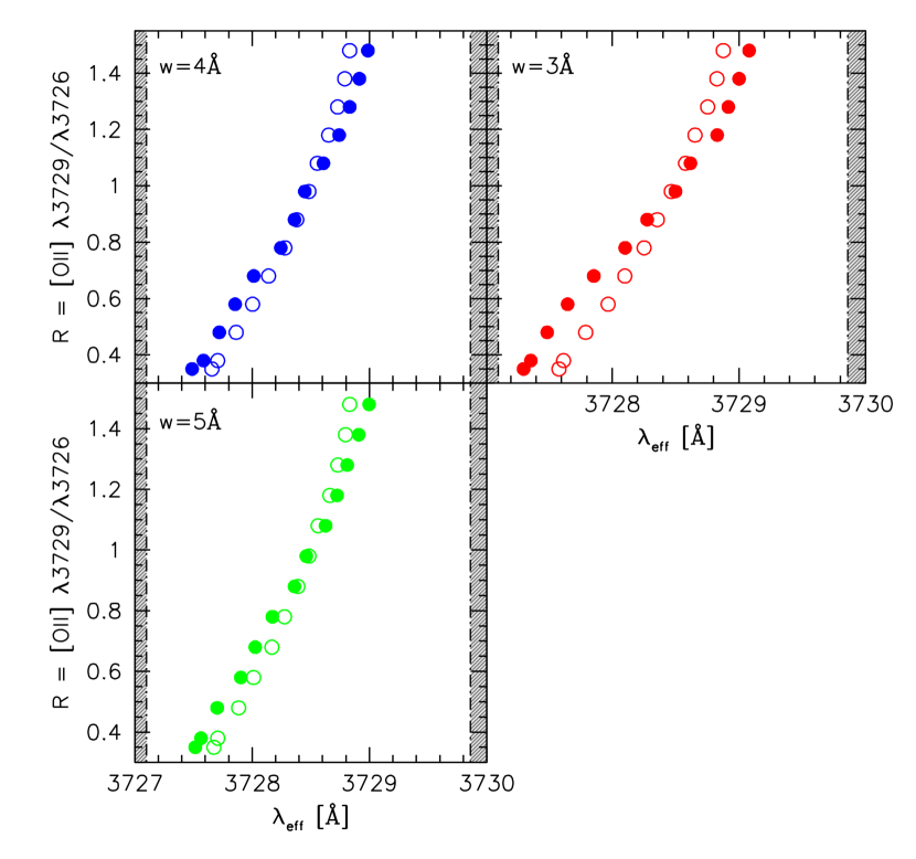
Figure 15: $\mathcal{R}$[OII] as a function of [Oii]$\lambda\lambda$3726,3729 doublet effective wavelength $\lambda_{\mathrm{eff}}$ for an unresolved mock doublet of FWHM 3, 4 and 5 Å. In each panel the open circles refer to Gaussian fits from the line base, filled circles from half peak intensity. The vertical dot-dashed lines mark the position of the individual component of the [Oii] doublet.

Table 6: Coefficients in equation 6

$w$	Fit	$k_{3}$	$k_{2}$	$k_{1}$	$k_{0}$
3	half	0.241	- 0.7672	+ 1.2428	+ 0.0302
3	full	0	0.3353	+ 0.0105	+ 0.2473
4	half	0	0.1831	+ 0.2726	+ 0.1818
4	full	0	0.4356	- 0.1684	+ 0.2879
5	half	0	0.1713	+ 0.3065	+ 0.1628
5	full	0	0.4492	- 0.2008	+ 0.2982

Table 7: Coefficients and limiting line ratios for [O ii] in equation 7

$\mathcal{R}$	$a$	$b$	$c$	$\mathcal{R}_{\rm min}^{a}$	$\mathcal{R}_{\rm max}^{b}$
[Oii]$\lambda$3729/$\lambda$3726	0.3771	2,468	638.4	0.3839	1.4558

^aTheoretical minimum line ratio calculated in the high-density limit of 100,000 cm^-3

^bTheoretical maximum line ratio calculated in the low-density limit of 1 cm^-3

So the $\lambda_{\mathrm{eff}}$ of [O ii] can be related to the density as follows:

$$\mathcal{R}(n_{\mathrm{e}})=k_{2}\lambda_{\mathrm{eff}}^{2}+k_{1}\lambda_{\mathrm{eff}}+k_{0}=a\frac{b+n_{\mathrm{e}}}{c+n_{\mathrm{e}}}$$ (8)

Making this relation explicit for density:

$$n_{\mathrm{e}}(\mathcal{R}) = \frac{c\mathcal{R}-ab}{a-\mathcal{R}}$$ (9)

$$n_{\mathrm{e}}(\lambda_{\mathrm{eff}}) = \frac{c(k_{2}\lambda_{\mathrm{eff}}^{2}+k_{1}\lambda_{\mathrm{eff}}+k_{0})-ab}{a-(k_{2}\lambda_{\mathrm{eff}}^{2}+k_{1}\lambda_{\mathrm{eff}}+k_{0})}$$ (10)

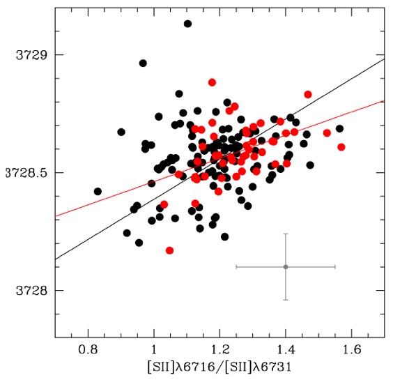
Figure 16: Relation between the [Oii]$\lambda$3727 effective wavelength $\lambda_{\mathrm{eff}}$ and the $R$[SII] intensity ratio for a sample of Hii regions. Red circles refer to a vetted subsample in which the uncertainty in the [Sii]$\lambda\lambda$6731,6717 doublet ratio $R$ is less than 10%. Best fitting lines are obtained with the bisector method (full sample, black line) and with an unweighted least square fit (vetted sample, blue line). Typical errors are $\delta\lambda_{\mathrm{eff}}\approx\pm 0.15$ Å for the effective wavelength and $\delta R$[SII]$\approx\pm 0.15$ for the [Sii]$\lambda\lambda$6731,6717 ratio.

An application of the method to the sample of Hii region from the SDSS DR1 by Kniazev et al. (2004) is shown in Fig. 16. The $\lambda_{\mathrm{eff}}$ and ${R}$[SII] are correlated. The scatter is relatively large. Typical errors ($\delta{R}$[SII] $\approx$ 0.15) suggest that measurement uncertainties account for most or all of it. If a restriction of $\delta R$[SII] $\lesssim$ 0.10 is applied, the correlation is better defined, with a Pearson correlation coefficient $r\approx 0.46$, implying a significance $\gtrsim 4\sigma$. The average value of ${R}$ [SII] and $\lambda_{\mathrm{eff}}$ [Oii]$\lambda$3727  are 1.21 and 3728.56 Å, respectively. The $R$ [SII] value implies $n_{\mathrm{e}}\approx 10^{2.4}$ cm^-3; $\lambda_{\mathrm{eff}}$ [Oii]$\lambda$3727 implies $\mathcal{R}$ [OII] $\approx 1.1$, which in turn yields $n_{\mathrm{e}}\approx 10^{2.5}$ cm^-3. The estimators are therefore consistent on average. This result indicates that, especially in some ideal cases, the $\lambda_{\mathrm{eff}}$ can be considered as a proxy of the [Oii]$\lambda$3727 doublet component ratio $\mathcal{R}$ and hence an appropriate $n_{\mathrm{e}}$ estimator.

References

- Abramowicz et al. (1988) Abramowicz, M. A., Czerny, B., Lasota, J. P., & Szuszkiewicz, E. 1988, ApJ, 332, 646
- Abramowicz & Straub (2014) Abramowicz, M. A. & Straub, O. 2014, Scholarpedia, 9, 2408
- Afanasiev & Popović (2015) Afanasiev, V. L. & Popović, L. Č. 2015, ApJ, 800, L35
- Barth et al. (2013) Barth, A. J., Pancoast, A., Bennert, V. N., et al. 2013, ApJ, 769, 128
- Bennert et al. (2018) Bennert, V. N., Loveland, D., Donohue, E., et al. 2018, MNRAS, 481, 138
- Bensch et al. (2015) Bensch, K., del Olmo, A., Sulentic, J., Perea, J., & Marziani, P. 2015, Journal of Astrophysics and Astronomy, 36, 467
- Bentz et al. (2013) Bentz, M. C., Denney, K. D., Grier, C. J., et al. 2013, ApJ, 767, 149
- Berton et al. (2016) Berton, M., Caccianiga, A., Foschini, L., et al. 2016, A&A, 591, A98
- Bian et al. (2012) Bian, W.-H., Fang, L.-L., Huang, K.-L., & Wang, J.-M. 2012, MNRAS, 427, 2881
- Boller et al. (1996) Boller, T., Brandt, W. N., & Fink, H. 1996, A&A, 305, 53
- Bon et al. (2016) Bon, E., Zucker, S., Netzer, H., et al. 2016, ApJS, 225, 29
- Bon et al. (2018) Bon, N., Bon, E., & Marziani, P. 2018, Frontiers in Astronomy and Space Sciences, 5, 3
- Bon et al. (2015) Bon, N., Bon, E., Marziani, P., & Jovanović, P. 2015, Ap&SS, 360, 7
- Bon et al. (2014) Bon, N., Popović, L. Č., & Bon, E. 2014, Advances in Space Research, 54, 1389
- Boroson (2002) Boroson, T. A. 2002, ApJ, 565, 78
- Boroson & Green (1992) Boroson, T. A. & Green, R. F. 1992, ApJS, 80, 109
- Brightman et al. (2019) Brightman, M., Bachetti, M., Earnshaw, H. P., et al. 2019, BAAS, 51, 352
- Canto et al. (1980) Canto, J., Meaburn, J., Theokas, A. C., & Elliott, K. H. 1980, MNRAS, 193, 911
- Capellupo et al. (2015) Capellupo, D. M., Netzer, H., Lira, P., Trakhtenbrot, B., & Mejía-Restrepo, J. 2015, MNRAS, 446, 3427
- Cid Fernandes et al. (2005) Cid Fernandes, R., Mateus, A., Sodré, L., Stasińska, G., & Gomes, J. M. 2005, MNRAS, 358, 363
- Collin et al. (2006) Collin, S., Kawaguchi, T., Peterson, B. M., & Vestergaard, M. 2006, A&Ap, 456, 75
- Condon et al. (1985) Condon, J. J., Hutchings, J. B., & Gower, A. C. 1985, AJ, 90, 1642
- Cracco et al. (2016) Cracco, V., Ciroi, S., Berton, M., et al. 2016, MNRAS, 462, 1256
- Czerny et al. (2018) Czerny, B., Beaton, R., Bejger, M., et al. 2018, Space Science Reviews, 214, #32
- Decarli et al. (2011) Decarli, R., Dotti, M., & Treves, A. 2011, MNRAS, 413, 39
- Dewangan et al. (2002) Dewangan, G. C., Singh, K. P., Gunn, K. F., et al. 2002, MNRAS, 337, 693
- Dimitrijević et al. (2007) Dimitrijević, M. S., Popović, L. Č., Kovačević, J., Dačić, M., & Ilić, D. 2007, MNRAS, 374, 1181
- Dong et al. (2011) Dong, X.-B., Wang, J.-G., Ho, L. C., et al. 2011, ApJ, 736, 86
- D’Onofrio & Burigana (2009) D’Onofrio, M. & Burigana, C. 2009, Questions of Modern Cosmology: Galileo’s Legacy (Springer Verlag)
- Du et al. (2015) Du, P., Hu, C., Lu, K.-X., et al. 2015, ApJ, 806, 22
- Du et al. (2016a) Du, P., Lu, K.-X., Hu, C., et al. 2016a, ApJ, 820, 27
- Du & Wang (2019) Du, P. & Wang, J.-M. 2019, ApJ, 886, 42
- Du et al. (2016b) Du, P., Wang, J.-M., Hu, C., et al. 2016b, ApJ, 818, L14
- Du et al. (2018) Du, P., Zhang, Z.-X., Wang, K., et al. 2018, ApJ, 856, 6
- Elvis et al. (1994) Elvis, M., Wilkes, B. J., McDowell, J. C., et al. 1994, ApJS, 95, 1
- Eracleous & Halpern (2004) Eracleous, M. & Halpern, J. P. 2004, ApJS, 150, 181
- Euclid Red Book Editorial Team (2011) Euclid Red Book Editorial Team. 2011, Euclid: definition study report No. SRE(2011)12 (ESA)
- Ferland et al. (2009) Ferland, G. J., Hu, C., Wang, J., et al. 2009, ApJ, 707, L82
- Ferland et al. (1998) Ferland, G. J., Korista, K. T., Verner, D. A., et al. 1998, PASP, 110, 761
- Ferrarese & Merritt (2000) Ferrarese, L. & Merritt, D. 2000, ApJ, 539, L9
- Ganci et al. (2019) Ganci, V., Marziani, P., D’Onofrio, M., et al. 2019, A&A, 630, A110
- Gaur et al. (2019) Gaur, H., Gu, M., Ramya, S., & Guo, H. 2019, A&A, 631, A46
- Ge et al. (2016) Ge, X., Bian, W.-H., Jiang, X.-L., Liu, W.-S., & Wang, X.-F. 2016, MNRAS, 462, 966
- Gebhardt et al. (2000) Gebhardt, K., Bender, R., Bower, G., et al. 2000, ApJ, 539, L13
- Grupe et al. (1999) Grupe, D., Beuermann, K., Mannheim, K., & Thomas, H.-C. 1999, A&A, 350, 805
- Grupe et al. (2010) Grupe, D., Komossa, S., Leighly, K. M., & Page, K. L. 2010, ApJS, 187, 64
- Heckman et al. (1981) Heckman, T. M., Miley, G. K., van Breugel, W. J. M., & Butcher, H. R. 1981, ApJ, 247, 403
- Hook (2013) Hook, I. M. 2013, Royal Society of London Philosophical Transactions Series A, 371, 20282
- Hu et al. (2015) Hu, C., Du, P., Lu, K.-X., et al. 2015, ApJ, 804, 138
- Jarvis & McLure (2006) Jarvis, M. J. & McLure, R. J. 2006, MNRAS, 369, 182
- Jiang et al. (2007) Jiang, L., Fan, X., Ivezić, Ž., et al. 2007, ApJ, 656, 680
- Kaasinen et al. (2017) Kaasinen, M., Bian, F., Groves, B., Kewley, L. J., & Gupta, A. 2017, MNRAS, 465, 3220
- Kakkad et al. (2018) Kakkad, D., Groves, B., Dopita, M., et al. 2018, A&A, 618, A6
- Kauffmann & Maraston (2019) Kauffmann, G. & Maraston, C. 2019, MNRAS, 489, 1973
- Kellermann et al. (1989) Kellermann, K. I., Sramek, R., Schmidt, M., Shaffer, D. B., & Green, R. 1989, AJ, 98, 1195
- Kniazev et al. (2004) Kniazev, A. Y., Pustilnik, S. A., Grebel, E. K., Lee, H., & Pramskij, A. G. 2004, ApJS, 153, 429
- Koleva et al. (2009a) Koleva, M., Prugniel, P., Bouchard, A., & Wu, Y. 2009a, A&A, 501, 1269
- Koleva et al. (2009b) Koleva, M., Prugniel, P., De Rijcke, S., Zeilinger, W. W., & Michielsen, D. 2009b, Astronomische Nachrichten, 330, 960
- Koleva et al. (2008) Koleva, M., Prugniel, P., Ocvirk, P., Le Borgne, D., & Soubiran, C. 2008, MNRAS, 385, 1998
- Kollmeier et al. (2017) Kollmeier, J. A., Zasowski, G., Rix, H.-W., et al. 2017, ArXiv e-prints, 1711.03234 [[arXiv]1711.03234]
- Komossa & Xu (2007) Komossa, S. & Xu, D. 2007, ApJ, 667, L33
- Komossa et al. (2008) Komossa, S., Xu, D., Zhou, H., Storchi-Bergmann, T., & Binette, L. 2008, ApJ, 680, 926
- Kormendy & Ho (2013) Kormendy, J. & Ho, L. C. 2013, Ann. Rev. Astron. Astroph., 51, 511
- Kormendy & Illingworth (1982) Kormendy, J. & Illingworth, G. 1982, ApJ, 256, 460
- Kriss (1994) Kriss, G. 1994, Astronomical Data Analysis Software and Systems III, A.S.P. Conference Series, 61, 437
- Kuraszkiewicz et al. (2004) Kuraszkiewicz, J. K., Green, P. J., Crenshaw, D. M., et al. 2004, ApJS, 150, 165
- Lawson & Hanson (1995) Lawson, C. L. & Hanson, R. J. 1995, Solving Least Squares Problems (Society for Industrial and Applied Mathematics)
- Letawe et al. (2007) Letawe, G., Magain, P., Courbin, F., et al. 2007, MNRAS, 378, 83
- Maddox (2018) Maddox, N. 2018, MNRAS, 480, 5203
- Marquardt (1963) Marquardt, D. W. 1963, Journal of the Society for Industrial and Applied Mathematics, 11, 431
- Martínez-Aldama et al. (2019) Martínez-Aldama, M. L., Czerny, B., Kawka, D., et al. 2019, ApJ, 883, 170
- Martínez-Aldama et al. (2018) Martínez-Aldama, M. L., Del Olmo, A., Marziani, P., et al. 2018, Frontiers in Astronomy and Space Sciences, 4, 65
- Marziani et al. (2019) Marziani, P., del Olmo, A., Martínez-Carballo, M. A., et al. 2019, A&A, 627, A88
- Marziani et al. (2018) Marziani, P., Dultzin, D., Sulentic, J. W., et al. 2018, Frontiers in Astronomy and Space Sciences, 5, 6
- Marziani et al. (2016) Marziani, P., Martínez Carballo, M. A., Sulentic, J. W., et al. 2016, Ap&SS, 361, 29
- Marziani & Sulentic (2012) Marziani, P. & Sulentic, J. W. 2012, NARev, 56, 49
- Marziani & Sulentic (2014) Marziani, P. & Sulentic, J. W. 2014, MNRAS, 442, 1211
- Marziani et al. (2010) Marziani, P., Sulentic, J. W., Negrete, C. A., et al. 2010, MNRAS, 409, 1033
- Marziani et al. (2013a) Marziani, P., Sulentic, J. W., Plauchu-Frayn, I., & del Olmo, A. 2013a, AAp, 555, 89, 16pp
- Marziani et al. (2013b) Marziani, P., Sulentic, J. W., Plauchu-Frayn, I., & del Olmo, A. 2013b, ApJ, 764 [[arXiv]1301.0520]
- Marziani et al. (2009) Marziani, P., Sulentic, J. W., Stirpe, G. M., Zamfir, S., & Calvani, M. 2009, A&Ap, 495, 83
- Marziani et al. (2001) Marziani, P., Sulentic, J. W., Zwitter, T., Dultzin-Hacyan, D., & Calvani, M. 2001, ApJ, 558, 553
- McConnell et al. (2011) McConnell, N. J., Ma, C.-P., Gebhardt, K., et al. 2011, Nature, 480, 215
- McLure & Dunlop (2001) McLure, R. J. & Dunlop, J. S. 2001, MNRAS, 327, 199