SIMULTANEOUS MAGNETIC POLAR CAP HEATING DURING A FLARING EPISODE FROM THE MAGNETAR
1RXS J170849.0-400910

Abstract

During a pointed 2018 NuSTAR observation, we detected a flare with a 2.2 hour duration from the magnetar 1RXS J170849.0$-$400910. The flare, which rose in $\sim 25$ seconds to a maximum flux 6 times larger than the persistent emission, is highly pulsed with an rms pulsed fraction of $53\%$. The pulse profile shape consists of two peaks separated by half a rotational cycle, with a peak flux ratio of $\sim$2. The flare spectrum is thermal with an average temperature of 2.1 keV. Phase resolved spectroscopy show that the two peaks possess the same temperature, but differ in size. These observational results along with simple light curve modeling indicate that two identical antipodal spots, likely the magnetic poles, are heated simultaneously at the onset of the flare and for its full duration. Hence, the origin of the flare has to be connected to the global dipolar structure of the magnetar. This might best be achieved externally, via twists to closed magnetospheric dipolar field lines seeding bombardment of polar footpoint locales with energetic pairs. Approximately 1.86 hours following the onset of the flare, a short burst with its own 3-minute thermal tail occurred. The burst tail is also pulsating at the spin period of the source and phase-aligned with the flare profile, implying an intimate connection between the two phenomena. The burst may have been caused by a magnetic reconnection event in the same twisted dipolar field lines anchored to the surface hot spots, with subsequent return currents supplying extra heat to these polar caps.

1 Introduction

Magnetars are a special subset of the isolated neutron star family. Most exhibit long spin-periods (2-12 s) and large spin down rates ($10^{-13}$-$10^{-11}$ Hz s^-1), implying dipole magnetic field strengths of the order of $10^{14}$ G (Kouveliotou et al. 1998). They are persistent X-ray emitters, with quasi-thermal spectra in the soft X-ray band and unique non-thermal hard X-ray tails extending beyond 100 keV. Given that the rotational energy loss rates of magnetars are typically $\sim 10^{33}$-$10^{34}$ erg s^-1, and therefore well below their soft and hard X-ray luminosities ($\gtrsim 10^{35}$ erg s^-1), the high energy emission of magnetars must be powered by a source other than rotation. This source is widely believed to be the decay of their large internal and perhaps external magnetic fields (see Olausen & Kaspi 2014; Turolla et al. 2015; Kaspi & Beloborodov 2017, for recent reviews).

The most distinctive of the magnetar properties is their erratic bursting activity, the most common of which are the short ($\sim 0.2$ s), hard X-ray/soft $\gamma$-ray bursts with quasi-thermal spectra. The peak luminosity of these bursts is in the range of $10^{37}$-$10^{42}$ erg s^-1, briefly dwarfing the persistent hard X-ray signals (e.g., Collazzi et al. 2015). These short bursts are at times followed by softer tails, lasting upward of few tens of minutes (e.g., Göǧüs et al. 2011; An et al. 2014). In rare occasions, short burst tails observed with RXTE exhibited a stronger persistent pulsed emission (e.g., Gavriil et al. 2006). More peculiar still, are the very energetic bursts observed from a handful of magnetars, the intermediate and giant flares with peak energies of the order of $10^{43}$ erg (e.g., Kouveliotou et al. 2001) and upward of $10^{46}$ erg (e.g., Hurley et al. 1999), respectively. These events are usually followed by a decaying thermal tail of duration a few hundred seconds pulsating at the pulse period of the source. Finally, often accompanying these bursts, magnetars enter an outburst episode, during which their underlying persistent emission is spectrally and temporally altered, with brighter and harder X-ray spectra, pulse profile changes, timing noise and/or glitches (e.g., Archibald et al. 2015; Camero et al. 2014; Younes et al. 2017a, b). The bursts may have an internal origin through crust-quakes (Thompson & Duncan 1995) or an external one caused by magnetic reconnection, akin to solar flares (Lyutikov 2015).

1RXS J170849.0$-$400910 (hereafter 1RXS J1708$-$40), is a magnetar with an 11 second period discovered with ASCA (Sugizaki et al. 1997). Subsequent measurement of its spin down $\dot{\nu}=-1.6\times 10^{-13}$ Hz s^-1 (Israel et al. 1999) implied a spin-down age of about 9 kyr and a surface polar magnetic field strength of $B\approx 9.3\times 10^{14}$ G. 1RXS J1708$-$40 is one of the brightest magnetars in the soft X-ray band with an absorbed 1-10 keV flux $\sim 4\times 10^{-11}$ erg s^-1 cm^-2. To date, it has remained one of the few magnetars to not exhibit any outburst activity in archival data (Olausen & Kaspi 2014), except for a brighter hard X-ray pulsed flux during one archival RXTE observation (Dib, & Kaspi 2014).

In this letter, we report on the first flaring activity from 1RXS J1708$-$40 detected during a 2018 NuSTAR observation. Section 2 summarizes our observation and data reduction. We report here in Section 3 only on the magnetar flaring results, for which we will use the persistent signal from the source for comparison purposes only; details of the persistent emission characteristics are deferred to a later paper. The findings are summarized and discussed in Section 4, focusing on the likely identification of two hot polar caps as the sites for the flaring activity. Throughout the paper we assume a distance to the source of 3.8 kpc (Durant & van Kerkwijk 2006).

2 Observations and data reduction

The Nuclear Spectroscopic Telescope Array (NuSTAR, Harrison et al. 2013) consists of two identical modules FPMA and FPMB operating in the energy range 3-79 keV. NuSTAR observed 1RXS J1708$-$40 on 2018 August 28 for a total of 100.8 ks. We perform the data reduction and analysis using nustardas version v1.8.0, HEASOFT version 6.25, and the calibration files version 20190627. We use the flags saacalc=1, saamode=strict, tentacle=yes to correct for enhanced background activity visible at the edges of some of the good time intervals immediately before or after entering the South Atlantic Anomaly (SAA). This resulted in a total livetime exposure of 92.8 ks. We extract source high-level science products, using a circular region with a 60^′′ radius, centered on the brightest pixel around the source sky location. We use a circular region of the same size on the same ccd as the source to extract background light curves and spectra. We use the task nuproducts to extract light curves and spectral files, including ancillary and response files. We correct all light curves for livetime, point spread function (PSF), and vignetting using nulccorr. We also correct all arrival times to the solar barycenter and to drifts in the NuSTAR clock caused by temperature variations (Harrison et al. 2013).

We perform the spectral analysis using XSPEC version 12.10.1f (Arnaud 1996). We use the abundances of Wilms et al. (2000), the photo-electric cross-sections of Verner et al. (1996), and the Tuebingen-Boulder interstellar medium absorption model (tbabs) to account for X-ray absorption in the direction of 1RXS J1708$-$40. We bin the spectra to have one count per bin and use the Cash statistic (C-stat) in XSPEC for model parameter estimation and error calculation, unless otherwise noted. We add a constant normalization to all our spectral models to take into account any calibration uncertainties between the two NuSTAR instruments, which we find to be around $7\%$. This is larger than the typical $2\%$ cross-calibration accuracy, and may simply caused by the counting statistics fully dominating the instrumental effects. Finally, we fix the hydrogen column density in all spectra to $N_{\rm H}=1.89\times 10^{22}$ cm^-2; the best fit value derived from the persistent emission spectral analysis of our observation (Younes et al. 2019 in prep.).

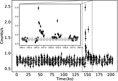
Figure 1: NuSTAR FPMA+FPMB 3-20 keV light curve of 1RXS J1708$-$40 binned at 150 s resolution. The grey horizontal solid and dashed lines delineate the average of the persistent emission and its $1\sigma$ uncertainty, respectively. The inset is a zoom-in of the dotted box region when enhanced emission above the persistent level is observed. See text for more details.

3 Results

The NuSTAR FPMA+FPMB 3-20 keV lightcurve of the source binned at a resolution of 150 s is shown in Figure 1. Enhanced emission is clearly present at around 147 ks from the start of the observation. The grey solid and dashed lines represent the average of the persistent emission and its $1\sigma$ uncertainty as derived from the beginning of the observation until the last Good Time Interval (GTI) before the start of the enhanced emission. The inset is a zoom-in of the dashed box-region around the time of the excess emission. The NuSTAR background level in the same energy range is at the 1.5% level of the persistent emission. Statistical inspection of the enhanced emission using a signal-to-noise method (e.g., Kaneko et al. 2010), at varying time resolutions, reveals a long flare-like event as the onset of the activity, and a short burst with its own tail 1.86 hours later. In the following sections, we first present the detailed analysis of the earlier enhanced emission, while we present the analysis of the short burst and its tail thereafter.

3.1 Early enhanced emission - Flare

3.1.1 Timing analysis

The earlier enhanced emission was visually inspected at multiple time-resolutions, starting at 0.128 s and up to 65 s. While we do find strong variability starting at 0.5 s time-scales, we find no evidence of an impulsive, short-like burst at the start of this enhanced emission, and the peak is only resolved at the $\gtrsim 8$ s resolution. Hence, we refrain from labelling this event as a burst to differentiate it from the typical magnetar short bursts; for the purposes of this paper we instead refer to it as a flare.

Figure 2 shows the 3-20 keV light curve encapsulating 3 long GTIs, the first of which includes the start of this enhanced emission (we note that the flare is not detected beyond 20 keV). The grey lines denote the persistent emission average and its 1$\sigma$ uncertainty. We exclude a 400 s interval during the second GTI, i.e., the hatched region, that covers the short burst and its tail. The red solid stair curve is the Bayesian blocks representation of the flare (Scargle et al. 2013). Emission above the level of the persistent one is seen up until the end of the 2nd GTI, 8 ks after the start of the flare. By the start of the third GTI, 2.6 ks later, the emission seems to have already declined back to within $1\sigma$ of the persistent emission.

To characterize the temporal properties of the flare, we fit the light curve shown in Figure 2 to 3 exponential functions, 1 for the rise and 2 for the decay (e.g., Gavriil et al. 2011). The fit is good with a $\chi^{2}_{\nu}$ of 1.1 for 265 degrees of freedom (dof). The properties are summarized in Table 1. We find a characteristic time-scale for the rise $\tau_{\rm r}=24\pm 3$ s, an initial decay $\tau_{\rm d}=52\pm 7$ s, and a shallower one $\tau_{\rm s}=1180\pm 180$ s. We find a duration $T90=3706\pm 316$ s.

Table 1: Temporal parameters

	$T_{0}$	$\tau_{r}$	$\tau_{d}$	$\tau_{s}$	$T90$
	MJD	s	s	s	s
Flare	58360.33620	$24\pm 3$	$54\pm 7$	$1180\pm 184$	$3706\pm 316$
Burst	58360.41281	$0.06\pm 0.01$	$0.04$	$0.58\pm 0.03$	$2.0$
Tail	58360.41287	$3$	$-$	$43\pm 5$	$137$

Notes. Parameters are estimated using a 32 s, 32 ms, and 16 s resolutions for the flare, the burst, and the burst-tail respectively. Parameters without error bars imply a $68\%$ upper-limit. In such case we do not quote any error on $T90$.

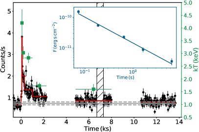
Figure 2: Flare FPMA+FPMB 3-20 keV light curve shown at the 32 s resolution. The grey horizontal lines (persistent emission) are as in Figure 1. The hatched region is a 400 s interval encapsulating the burst and its tail and was excluded from the flare analysis. The red stair curve is the Bayesian blocks representation of the flare. The right green axis and the green squares represent the BB temperature from time-resolved spectroscopy of the flare. The inset is the corresponding 3-20 keV absorption-corrected flux. The line is the best fit $t^{-\alpha}$ PL decay of the flux with an index $\alpha=0.84\pm 0.06$.

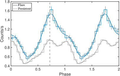
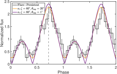
Figure 3: Left panel. Flare and persistent emission pulse profiles shown as blue and grey histograms, respectively, along with $1$ sigma error bars. The solid lines are Fourier fits including the first three harmonics. Right panel. Persistent-subtracted flare pulse profile, with the y-axis being counts normalized to the phase-averaged value. The light orange and purple curves are the profiles from a simple two-pole hot spot model with cap sizes $\theta_{\rm cap}=20^{\circ}$ and $1^{\circ}$, respectively. The model pulse profiles are for magnetic inclination $\alpha=60^{\circ}$. In both panels, the vertical dashed line is at $\phi_{\rm p}=0.72$, the phase of the first peak of the persistent emission pulse profile.

The flare pulse profile folded at the pulse frequency from the source (0.09081755(3), Younes et al. in prep.) is shown in blue in Figure 3. For comparison purposes, we also show the persistent emission pulse profile in grey. The solid lines overlaid on both curves are a Fourier series fit that includes contribution from the first three harmonics. The difference in the pulse profile shapes of the flare and the persistent emission implies that they are both pulsed. Assuming that the persistent emission temporal (and spectral) properties did not change during the flare emission, we subtracted the persistent emission profile from the flare one (i.e., assuming that the persistent emission is the background), which resulted in the profile shown in the right panel of Figure 3. We derive an rms pulsed fraction for the flare-only pulse profile of $53\pm 5\%$.

The flare pulse profile consists of two peaks with different brightness. We fit two Gaussians to the pulse profile which resulted in a good fit with $\chi^{2}_{\nu}$ of 0.7 for 11 dof (note that a single Gaussian fit results in $\chi^{2}_{\nu}$ of 1.8 for 14 dof with strong residuals at phases $<0.5$). From this model, we derive a peak separation of $0.55\pm 0.04$ cycles, i.e., half a rotation. The main and subsidiary peaks are detected at rotational phases $0.74\pm 0.02$ and $0.18\pm 0.03$, respectively. The brighter peak is aligned with the first peak of the persistent emission profile; the peak that dominates the emission below few keV (den Hartog et al. 2008), and is thermal in nature. We also searched for any variability in the pulse profile with energy. We built pulse profiles in two energy ranges, 3-8 and 8-20 keV. We find no discernable difference in shape. The pulse fraction at high energies is slightly larger at $60\pm 9\%$ compared to $51\pm 7\%$ at low energies.

We also performed time-resolved pulse profile analysis. We folded the light curve in each Bayesian block of Figure 2, starting from the peak and up to 8 ks, at the source pulse period. The pulse profile shape evolves from a broad pulse encompassing both peaks, to a double peaked profile. Given the low statistics of each pulse profile, measuring the pulsed fraction resulted in large error bars. Hence, we merged the first three bins and the last two to construct two relatively high signal-to-noise pulse profiles. We find that the pulsed fraction at earlier times is $38\pm 6\%$, markedly lower compared with the last two Bayesian-block bins which returned a pulsed fraction of $72\pm 9\%$. Finally, we searched for Giant-flare like transient quasi-periodic oscillations in the range 18 Hz to about 625 Hz (Israel et al. 2005; Huppenkothen et al. 2014) during the flare. We find no significant detection. That may be partially due to the very low signal-to-noise data in the flare for such an analysis, which also hindered any meaningful upper-limit measurement.

3.1.2 Spectral analysis

We fit the 4-20 keV time and phase averaged, persistent-emission corrected, flare spectrum with a power-law (PL) and a blackbody (BB) model. Given the relatively large total number of flare counts ($\sim 1500$ FPMA+FPMB), we group the spectra to have a minimum of 70 counts per bin and used the $\chi^{2}$ statistic. The BB model resulted in a better fit compared to the PL model with a $\chi^{2}_{\nu}$ of 1.03 and 1.3, respectively, for 44 dof. We find a BB temperature $kT=2.14\pm 0.12$ keV and a 3-20 keV flux $F_{\rm 3-20~{}keV}=(1.00\pm 0.07)\times 10^{-11}$ erg s^-1 cm^-2, which is $36\%$ of the persistent emission flux in the same energy range. Assuming circular geometry, we derive a phase-averaged radius for the emitting region $R=84_{-9}^{+11}$ m. We summarize the best fit parameters of both models in Table 2.

For spectroscopy including the higher energy window above 20 keV, we added a PL component to the BB one, and thereby derived an upper-limit on the detection of a putative hard X-ray tail component for the flare. We fixed the PL $\Gamma$ to 0.7, similar to the one we derive for the persistent emission during this observation. The BB temperature and normalization were left free to vary. We obtained an upper limit $F_{\rm 20-70~{}keV}\lesssim 8\times 10^{-12}$ erg s^-1 cm^-2. This is $52\%$ of the 20-70 keV persistent flux. Given that the increase in the 3-20 keV flux during the flare was at the $36\%$ level, one cannot exclude the possibility for such an increase/flare to have occurred in the hard PL as well.

A time-resolved spectral analysis of the flare was performed by fitting a BB model to each of the Bayesian block bins, starting from the peak. This revealed a strong cooling trend throughout the flare with the temperature decreasing from $4.2\pm 0.5$ keV to $1.6\pm 0.2$ keV. On the other hand, no significant change appeared in the area of the BB emitting region. The 3-20 keV flux decreases from $(1.55\pm 0.20)\times 10^{-10}$ erg s^-1 cm^-2 to $3.7_{-0.7}^{+0.6}\times 10^{-12}$ erg s^-1 cm^-2. The flux decay is well fit with a PL function $F(t)\propto t^{-\alpha}$ with $\alpha=0.84\pm 0.06$. The temperature and flux decay trends are shown in Figure 2, while all spectral parameters are summarized in Table 2. We derive a flare fluence $\Phi=(7.0\pm 0.6)\times 10^{-8}$ erg cm^-2 and a total emitted energy $E=(1.2\pm 0.1)\times 10^{38}$ erg, which is about $50\%$ of the energy emitted in the persistent emission in the same time-span.

Finally, we carried out phase-resolved spectroscopic analysis of the source. We divided the pulse profile into three bins encapsulating the two peaks and the interpulse emission (Table 2). The BB temperature is consistent within $1\sigma$ between the two peaks, whereas, the area of the emitting region is a factor of 2.7 smaller in the weaker pulse compared to the main one. The interpulse spectrum exhibits a slightly smaller temperature than the pulses and an area comparable to the size of the main pulse.

Table 2: Spectral parameters

	Model	$kT$	$\Gamma$	$R$	$F$	$L$	$\chi^{2}$/dof	Cstat/dof
		(keV)		(m)	erg s-1 cm-2	erg s-1
Flare
0.0-1.0	BB	$2.14\pm 0.12$	$-$	$84_{-9}^{+11}$	$10_{-0.8}^{+0.6}$	$1.7\pm 0.1$	45/44	$-$
0.0-1.0	PL	$-$	$2.12\pm 0.13$	$-$	$12\pm 1$	$2.1\pm 0.2$	45/44	$-$
Time-resolved spectroscopy
Bin 1	BB	$4.2_{-0.4}^{+0.6}$	$-$	$97_{-15}^{+23}$	$155_{-22}^{+21}$	$27\pm 3$	$-$	100/111
Bin 2	BB	$3.0_{-0.2}^{+0.3}$	$-$	$101_{-13}^{+17}$	$55\pm 6$	$9.5\pm 1.0$	$-$	235/268
Bin 3	BB	$2.8\pm 0.2$	$-$	$76\pm 10$	$23\pm 2$	$4.0\pm 0.3$	$-$	360/426
Bin 4	BB	$1.7_{-0.1}^{+0.2}$	$-$	$133_{-18}^{+27}$	$9\pm 1$	$1.6\pm 0.2$	$-$	407/430
Bin 5	BB	$1.6\pm 0.2$	$-$	$100_{-20}^{+40}$	$3.7\pm 0.6$	$0.64\pm 0.10$	$-$	585/593
Phase-resolved spectroscopy
0.06-0.28	BB	$2.3\pm 0.2$	$-$	$64_{-11}^{+17}$	$8_{-2}^{+1}$	$1.4_{-0.3}^{+0.2}$	$-$	404/472
0.56-0.94	BB	$2.2\pm 0.1$	$-$	$105\pm 10$	$17_{-1}^{+2}$	$2.9_{-0.2}^{+0.4}$	$-$	472/575
Rest	BB	$1.8\pm 0.2$	$-$	$98_{-19}^{+30}$	$6.4_{-0.9}^{+0.8}$	$1.1\pm 0.1$	$-$	424/489
Burst
0.0-1.0	BB	$6.2_{-0.8}^{+1.2}$	$-$	$180_{35}^{+45}$	$3200_{-600}^{+800}$	$550_{-100}^{+140}$	$-$	60/61
0.0-1.0	PL	$-$	$0.6\pm 0.2$	$-$	$3900_{-800}^{+900}$	$670_{-130}^{+160}$	$-$	54/61
Tail
0.0-1.0	BB	$2.9_{-0.4}^{+0.5}$	$-$	$80\pm 20$	$34_{-8}^{+7}$	$6\pm 1$	$-$	154/163
0.0-1.0	PL	$-$	$1.7_{-0.2}^{+0.3}$	$-$	$53_{-0.7}^{+0.6}$	$9\pm 1$	$-$	155/163

Notes. The first column represents the time bins (Figure 2) or rotational phase intervals for which the spectral analysis is performed. Fluxes are in units of $10^{-12}$ erg s^-1 cm^-2 and derived in the energy range 3-20 keV, except for the short burst, for which we report the 3-35 keV flux. Radii and luminosities are derived by adopting a 3.8 kpc distance (Durant & van Kerkwijk 2006), and the latter is in units of $10^{34}$ erg s^-1. All listed uncertainties are at the $1\sigma$ level.

3.2 Short burst and tail

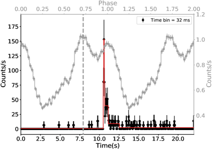
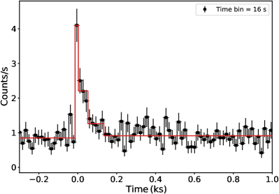
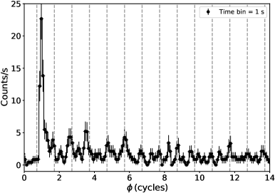
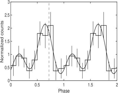
Figure 4: Upper-left panel. Short burst light curve shown at the 32 ms time-scale. The red stair curve is the burst Bayesian blocks representation. The start time of the light curve corresponds to T0 at which phase=0, shifted by a time equivalent to 12915 rotations. The end time is 2 rotations later. The grey curve is a high resolution persistent emission pulse profile. Two rotations are shown. The grey vertical dashed line corresponds to $\phi_{\rm p}=0.72$. Upper-right panel. Burst light curve shown at the 16 s time-scale, with its Bayesian blocks representation in red. Lower-left panel. Burst light curve shown at the 1.0 s time-scale, 1/11th of 1RXS J1708$-$40 rotational period. The x-axis is in rotational phase $\phi$ normalized by $2\pi$ (i.e., cycles). The start phase corresponds to $\phi$=0, shifted by 12915 rotations. The vertical dashed grey lines are drawn at $\phi=\phi_{\rm p}+n$, with $n$ an integer from 0 to 14. Lower-right panel. Folded light curve of the burst tail shown in the lower-left panel, excluding a 2 s interval around the burst time. Grey vertical dashed line corresponds to $\phi_{\rm p}$. See text for more details.

We plot the short burst light curve at the 32 ms time-scale in the upper-left panel of Figure 4. The full time interval that is shown spans two rotational periods. The start time of the light curve corresponds to T0 at which phase=0 (see Section 3), shifted by a time equivalent to an integer number of rotations (12915). The end time is two rotations later. To identify the phase at which the burst occurred, we plot in grey two cycles of the persistent emission pulse profile. The burst aligns with the second peak of that profile, which fully dominates the emission at energies $>20$ keV. We fit the burst light curve to 3 exponential functions using a maximum-likelihood method. We measure $T90\approx 2$ s. The right panel of Figure 4 shows the burst light curve at 16 s resolution. Only 2 exponential functions are required to fit this light curve, and we measure a $T90\approx 140$ s. The temporal properties of this burst and its tail are summarized in Table 1.

The light curve of the burst tail at 1 s resolution (one-eleventh of the rotational period of 1RXS J1708$-$40) is shown in the lower-left panel of Figure 4. Phase 0 corresponds to T0, shifted by 12915 rotations. The dashed vertical lines are at $\phi=\phi_{\rm p}+n$ with $n$ an integer from 0 to 14. Peaks during the tail light curve are clearly seen aligned at $\phi$, with a small hint of interpulses. We folded the same light curve at the spin period from the source and subtracted the persistent emission pulse profile. The result is shown in the right panel of Figure 4. The pulse is detected at the $4.8\sigma$ level. Fitting a two Gaussian model to the pulse profile, we find the phases of the main and secondary peaks at $0.65\pm 0.10$ and $0.18\pm 0.10$, respectively. These phases are within 1$\sigma$ uncertainty from the flare pulse peaks (Section 3.1.1). Moreover, their peak flux ratio of about 2 is also consistent with that of the flare. While the secondary peak is not, on its own, statistically significant, its appearance at the same rotational phase as the minor peak in the flare pulse profile and at the same flux level enhance confidence in the reality of its existence.

We fit the short-burst 3-40 keV phase-averaged spectrum with a BB and a PL model. The former results in a CSTAT of 60 for 61 dof. We find a BB temperature $kT=6.2_{-0.8}^{+1.2}$ and a radius for the emitting region $R=180_{-35}+{45}$ m. The BB 3-40 keV flux is $3.2_{{}_{-}0.6}^{+0.8}\times 10^{-9}$ erg s^-1 cm^-2. The PL model results in a slightly better fit with a CSTAT of 54 for 61 dof. We find a photon index $\Gamma=0.6\pm 0.2$ and a 3-40 keV flux of $3.9_{{}_{-}0.8}^{+0.9}\times 10^{-9}$ erg s^-1 cm^-2. This implies a burst fluence of about $7.8\times 10^{-9}$ erg cm^-2. Bursts analyzed with Swift/BAT or Fermi/GBM usually require either a cutoff at high energies or, more accurately, are best fit with a 2 BB model (Lin et al. 2012; Younes et al. 2014). This extra component is not required in our data, which could be attributed to the lower sensitivity of NuSTAR at energies beyond 30 keV. Finally, we fit the 4-20 keV tail spectrum with a PL and a BB model. The PL model results in CSTAT of 155 for 163 dof. We find a photon index $\Gamma=1.7\pm 0.2$ and a 3-20 keV flux of $3.5_{-0.8}^{+0.6}\times 10^{-11}$ erg cm^-2 s^-1. The BB model gives a CSTAT of 154 for 163 dof, a phase-averaged temperature $kT=2.9\pm 0.4$ keV with radius $R=80\pm 20$ m. The former is slightly larger than the temperature in the flare, whereas both possess a similar area. We find a 3-20 keV flux $F=(2.9\pm 0.6)\times 10^{-11}$ erg cm^-2 s^-1. The fluence in the tail of the burst is $\Phi_{\rm t}=5.2\times 10^{-9}$ erg cm^-2. Hence, the energy emitted by 1RXS J1708$-$40 during the burst and its tail is $\sim 1.8\times 10^{37}$ erg; an order of magnitude smaller than the total energy emitted during the flare.

4 Summary and discussion

In this Letter, we report on flaring activity from the magnetar 1RXS J1708$-$40, which, until now, had not shown any of the bursting behaviors common to this class of sources. The transient activity lasted about 2.2 hours with $T_{90}\approx 1$ hr and a rise time of $\tau_{\rm r}=24$ s. It was not triggered by any impulsive event, such as a short burst, and no unusual activity was apparent prior to the flare. Such enhanced emission in magnetars has been seen after giant and intermediate flares (Hurley et al. 1999; Ibrahim et al. 2001; Palmer et al. 2005, e.g.,), short milli-second bursts (Woods et al. 2005; Gavriil et al. 2011; An et al. 2014), and at the onset of a major bursting episode (Kaneko et al. 2010). Hence, the enhanced emission discussed here demonstrates that long-duration, low-level activity could also happen in isolation, and it may be quasi-continuous in at least some magnetars (see also Esposito et al. 2019).

A unique aspect to the 1RXS J1708$-$40 flare is its highly pulsed nature, with a pulse profile differing in shape from the persistent emission one. It consists of two peaks separated by half a cycle, with a flux ratio of two. The brighter peak coincides in phase with the quasi-thermal, soft emission ($\lesssim 4$ keV) peak of the persistent pulse profile (e.g., den Hartog et al. 2008). Its rms pulse fraction is $53\%$; a factor two larger than the persistent emission one ($PF=28\%$). Finally, the two peaks in the flare pulse profile are present throughout the whole episode of activity, and with similar flux ratio.

The time-integrated, phase-averaged flare spectrum is best fit with a thermal blackbody model of temperature $kT=2.1$ keV, which is 4.5 times higher than the persistent emission blackbody temperature (e.g., Rea et al. 2005). The effective area of the emitting region, with a radius $R\approx 100$ m, is much smaller than that of the persistent emission ($R_{\rm per}\approx 2$ km, Rea et al. 2005). We cannot exclude the presence of a similar transient hard X-ray component in our data if the increase is at a similar level as the 3-20 keV flux. Phase-resolved spectroscopy of the flare reveals that both peaks are thermal with similar BB temperatures of about 2.1 keV. They only differ in the apparent size of their emitting area.

The flare double-peaked pulse profile with peak separation of half a rotation (Fig. 3), the appearance of the two peaks at the flare onset and for its full duration, and the peaks similar BB temperature strongly suggest simultaneous heating to two antipodal surface spots with the same population of energetic particles.The most natural regions on the magnetar surface are the two magnetic polar caps, since areas connected to higher-order fields are usually threading footprints with closer proximity on the surface. To test this hypothesis, we developed a simple two-polar hot spot model for generating pulsed emission profiles. The identical surface spots were centered at opposite poles, and spanned magnetic colatitudes between zero and $\theta_{\rm cap}$, and $\pi$ and $\pi-\theta_{\rm cap}$. Results for $\theta_{\rm cap}=1^{\circ},20^{\circ}$ are illustrated in Fig. 3, though profiles for a full range of $0<\theta_{\rm cap}\leq\pi/2$ were surveyed.

The hot spots emitted uniformly across their surfaces. A simple anisotropic and azimuthally-symmetric emission flux profile of ${\cal F}(\theta_{z})={\cal F}_{0}(1+\sin^{2}\theta_{z})^{-\beta}$ was assumed at each point on each cap, with $\theta_{z}$ representing the local zenith angle. This choice is motivated by general expectations of radiative transfer in highly-magnetic neutron star atmospheres. The zenith flux ${\cal F}_{0}$ was fixed for all pulse profile simulations, and the anisotropy index $\beta$ allowed to vary from $\beta=0$ (isotropy) to $\beta=4$ (pencil-beam like). The two other key parameters for controlling pulse profile morphology are the angle $\alpha$ between the magnetic dipole and rotation axes, and the angle $\zeta$ of the observer viewing direction to the magnetar rotation axis. The simulations were performed for flat spacetime to aid expediency of the analysis.

A broad array of pulse profiles was thus generated. The special cases of an orthogonal rotator ($\alpha=90^{\circ}$) or equatorial viewing ($\zeta=90^{\circ}$) generate two identical peaks that do not match the observations. Low values of $\zeta\lesssim 50^{\circ}$ occult the antipodal (remote) polar cap so that only a single peak emerges. The relative heights of the two peaks (each symmetric) and their widths were used to constrain the parameters $\alpha$, $\zeta$ and $\beta$. This survey revealed that $\alpha\sim 60^{\circ}$ and $\zeta\sim 60^{\circ}$ as displayed in the right panel of Fig. 3 generated the best fit, with a reduced $\chi^{2}$ of $1.7$ for $\theta_{\rm cap}=20^{\circ}$ (orange curve), and $\chi^{2}$ of 2.2 for $\theta_{\rm cap}=1^{\circ}$ (purple). The tolerance in these values was around $\pm 10^{\circ}$, albeit with an anti-correlation between $\alpha$ and $\zeta$ choices. The best-fit $\beta$ index was $1/2$, indicating very modest surface anisotropy, though we note that the larger values of $\beta=1-2$ narrowed the peaks only modestly. It is evident that reducing the $\theta_{\rm cap}$ value to around $1^{\circ}$ narrows the peaks slightly and increases the pulse fraction somewhat. Note that the $\theta_{\rm cap}=1^{\circ}$ case lowers the effective spot radius to $\sim 174$ m (for a stellar radius of 10 km), i.e., much closer to that estimated from the observed flux.

The quality of the fit is sufficient to indicate approximate consistency of the two-polar cap scenario with the observed pulse profile. Refined treatment of curved photon trajectories is expected to modify the fit parameters only by fairly small fractions. The main general relativistic manifestations are to increase the effective brightness of the antipodal cap somewhat and enlarge the range of phases for which this cap is visible. These influences enhance and broaden the subsidiary peak slightly so as to effectively reduce the pulsed fraction. A more detailed modeling of the flare light curve including all the above is deferred to future work.

The large value of $\alpha$ obtained here contrasts that found for 1E 1841-045 ($\alpha\approx 15^{\circ}$ An et al. 2015) and also $\alpha\sim 0^{\circ}$ identified for 1RXS J1708$-$40 (Hascoët et al. 2014) from spectral modeling of magnetospheric hard X-ray tail emission. Results in those two papers emphasize phase-averaged spectral fitting using the magnetic Thomson scattering model of Beloborodov (2013). The strong dependence of such resonant upscattering spectra on pulse phase (e.g., Wadiasingh et al. 2018, see also Fig. 7 of Beloborodov 2013) renders spectral similitude a relatively poor probe of the geometric angles $\alpha$ and $\zeta$. Pulse profile comparison between data and model is a more precise diagnostic for these angles. Such was emphasized in the flat spacetime pulse profile fitting of XMM data below 10 keV performed by Albano et al. (2010) for two magnetars. They found that $\alpha\sim 20^{\circ}$ for XTE J1810-197 with its simple, single-peaked pulsation, and $\alpha\sim 85^{\circ}$ for CXOU J164710.2$-$455216 with its multi-peaked pulse profile; more along the lines of the geometry constraints derived in this paper.

The main question now is, how is it possible to heat both magnetic polar caps simultaneously at the onset of the flare and for the length of its decay? While this can potentially happen in subsurface zones, the observed antipodal heating demands that the site for activation has a prompt/simultaneous physical connection to both poles. This is likely difficult to achieve below the surface given the diffusive nature of heat transport. Collective energy transfer mediated by acoustic or Alfvénic modes may provide an alternative possibility, but would require a specialized transport geometry below the surface.

For a magnetospheric origin, dipolar fields may undergo large twists, perhaps due to a shift in the underlying crustal area to which they are anchored. The toroidal components to these fields generate strong electric fields that rapidly accelerate magnetospheric electrons ejected from the surface, precipitating prolific pair creation. The resultant over-twisting is unsustainable for long, and will naturally relax with an evolution progressing towards quasi-polar field-line footpoints (Chen & Beloborodov 2017). Pairs accelerated in the twisted field zones bombard the polar surface regions (e.g., Beloborodov & Li 2016; González-Caniulef et al. 2019), so that accompanying enhanced heating of both polar caps simultaneously is naturally expected. Twists in dipolar magnetic fields, however, are also believed to power non-thermal hard X-ray emission (e.g., Beloborodov 2013; Wadiasingh et al. 2018). Assuming that the increase in this component is at the level of the soft thermal emission, its non-detection is then expected given the upper-limit we derive on the 20-70 keV flare flux (Section 3.1.2).

The temporal and spectral properties of the short burst detected from 1RXS J1708$-$40 towards the end of the flare is typical of magnetar short bursts observed with NuSTAR (e.g., An et al. 2014). The burst time is phase-locked with the second peak of the persistent pulsed emission which completely dominates above $20$ keV (Figure 4, den Hartog et al. 2008). It occurs at the flare pulse profile phase minimum, and so may not be associated with either pole. The short burst is followed by a 3 minute tail, well fit with a BB model having phase-averaged $kT\sim 3$ keV and $R\sim 80$ m. The temperature is larger than the one derived for the flare spectrum, while the radii are consistent. Moreover, the tail is pulsating at the spin period of the source, with a pulse profile aligning in phase with that of the flare and exhibiting a similar pulsed fraction.

The above common characteristics between the flare and the burst tail point to an intimate connection between the origin of both events. They are naturally explained if the burst also occurred in the magnetosphere, on the same field loops anchored to the initial heated magnetic polar cap areas. These loops experienced a twist at the onset of the activity that perhaps precipitated a magnetic reconnection event (Lyutikov 2015), causing the burst. Return currents deposit extra heat onto the same surface region, resulting in an increase in the surface temperature without impacting the size of the emitting area. In summary, the flare observations persent here provide strong evidence for a twist to the global dipolar magnetic field as the source of activation in 1RXS J1708$-$40, and perhaps in other magnetars. They also point to twists as the source for short bursts, perhaps through magnetic reconnection in the magnetosphere.

References

- Albano et al. (2010) Albano, A., Turolla, R., Israel, G. L., et al. 2010, ApJ, 722, 788
- An et al. (2015) An, H., Archibald, R. F., Hascoët, R., et al. 2015, ApJ, 807, 93
- An et al. (2014) An, H., Kaspi, V. M., Beloborodov, A. M., et al. 2014, ApJ, 790, 60
- Archibald et al. (2015) Archibald, R. F., Kaspi, V. M., Ng, C.-Y., et al. 2015, ApJ, 800, 33
- Arnaud (1996) Arnaud, K. A. 1996, in ASP Conf. Ser. 101: Astronomical Data Analysis Software and Systems V, 17
- Beloborodov (2013) Beloborodov, A. M. 2013, ApJ, 762, 13
- Beloborodov & Li (2016) Beloborodov, A. M. & Li, X. 2016, ArXiv e-prints
- Camero et al. (2014) Camero, A., Papitto, A., Rea, N., et al. 2014, MNRAS, 438, 3291
- Chen & Beloborodov (2017) Chen, A. Y. & Beloborodov, A. M. 2017, ApJ, 844, 133
- Collazzi et al. (2015) Collazzi, A. C., Kouveliotou, C., van der Horst, A. J., et al. 2015, The Astrophysical Journal Supplement Series, 218, 11
- den Hartog et al. (2008) den Hartog, P. R., Kuiper, L., & Hermsen, W. 2008, A&A, 489, 263
- Dib, & Kaspi (2014) Dib, R., & Kaspi, V. M. 2014, ApJ, 784, 37
- Durant & van Kerkwijk (2006) Durant, M. & van Kerkwijk, M. H. 2006, ApJ, 650, 1070
- Esposito et al. (2019) Esposito, P., De Luca, A., Turolla, R., et al. 2019, A&A, 626, A19
- Gavriil et al. (2011) Gavriil, F. P., Dib, R., & Kaspi, V. M. 2011, ApJ, 736, 138
- Gavriil et al. (2006) Gavriil, F. P., Kaspi, V. M., & Woods, P. M. 2006, ApJ, 641, 418
- González-Caniulef et al. (2019) González-Caniulef, D., Zane, S., Turolla, R., & Wu, K. 2019, MNRAS, 483, 599
- Göǧüs et al. (2011) Göǧüs, E., Woods, P. M., Kouveliotou, C., et al. 2011, ApJ, 740, 55
- Harrison et al. (2013) Harrison, F. A., Craig, W. W., Christensen, F. E., et al. 2013, ApJ, 770, 103
- Hascoët et al. (2014) Hascoët, R., Beloborodov, A. M., & den Hartog, P. R. 2014, ApJ, 786, L1
- Huppenkothen et al. (2014) Huppenkothen, D., Watts, A. L., & Levin, Y. 2014, ApJ, 793, 129
- Hurley et al. (1999) Hurley, K., Cline, T., Mazets, E., et al. 1999, Nature, 397, 41
- Ibrahim et al. (2001) Ibrahim, A. I., Strohmayer, T. E., Woods, P. M., et al. 2001, ApJ, 558, 237
- Israel et al. (2005) Israel, G. L., Belloni, T., Stella, L., et al. 2005, ApJ, 628, L53
- Israel et al. (1999) Israel, G. L., Covino, S., Stella, L., et al. 1999, ApJ, 518, L107
- Kaneko et al. (2010) Kaneko, Y., Göğüş, E., Kouveliotou, C., et al. 2010, ApJ, 710, 1335
- Kaspi & Beloborodov (2017) Kaspi, V. M. & Beloborodov, A. 2017, ArXiv e-prints
- Kouveliotou et al. (1998) Kouveliotou, C., Dieters, S., Strohmayer, T., et al. 1998, Nature, 393, 235
- Kouveliotou et al. (2001) Kouveliotou, C., Tennant, A., Woods, P. M., et al. 2001, ApJ, 558, L47
- Lin et al. (2012) Lin, L., Göğüş, E., Baring, M. G., et al. 2012, ApJ, 756, 54
- Lyutikov (2015) Lyutikov, M. 2015, MNRAS, 447, 1407
- Olausen & Kaspi (2014) Olausen, S. A. & Kaspi, V. M. 2014, ApJS, 212, 6
- Palmer et al. (2005) Palmer, D. M., Barthelmy, S., Gehrels, N., et al. 2005, Nature, 434, 1107
- Rea et al. (2005) Rea, N., Oosterbroek, T., Zane, S., et al. 2005, Monthly Notices of the Royal Astronomical Society, 361, 710
- Scargle et al. (2013) Scargle, J. D., Norris, J. P., Jackson, B., & Chiang, J. 2013, ApJ, 764, 167
- Sugizaki et al. (1997) Sugizaki, M., Nagase, F., Torii, K., et al. 1997, PASJ, 49, L25
- Thompson & Duncan (1995) Thompson, C. & Duncan, R. C. 1995, MNRAS, 275, 255
- Turolla et al. (2015) Turolla, R., Zane, S., & Watts, A. L. 2015, Reports on Progress in Physics, 78, 116901
- Verner et al. (1996) Verner, D. A., Ferland, G. J., Korista, K. T., & Yakovlev, D. G. 1996, ApJ, 465, 487
- Wadiasingh et al. (2018) Wadiasingh, Z., Baring, M. G., Gonthier, P. L., & Harding, A. K. 2018, ApJ, 854, 98
- Wilms et al. (2000) Wilms, J., Allen, A., & McCray, R. 2000, ApJ, 542, 914
- Woods et al. (2005) Woods, P. M., Kouveliotou, C., Gavriil, F. P., et al. 2005, ApJ, 629, 985
- Woods et al. (2001) Woods, P. M., Kouveliotou, C., Göğüş, E., et al. 2001, ApJ, 552, 748
- Younes et al. (2017a) Younes, G., Baring, M. G., Kouveliotou, C., et al. 2017a, ApJ, 851, 17
- Younes et al. (2017b) Younes, G., Kouveliotou, C., Jaodand, A., et al. 2017b, ApJ, 847, 85
- Younes et al. (2014) Younes, G., Kouveliotou, C., van der Horst, A. J., et al. 2014, ApJ, 785, 52