Semi-analytic forecasts for JWST – IV. Implications for cosmic reionization and LyC escape fraction

Abstract

Galaxies forming in low-mass halos are thought to be primarily responsible for reionizing the Universe during the first billion years after the Big Bang. Yet, these halos are extremely inefficient at forming stars in the nearby Universe. In this work, we address this apparent tension, and ask whether a physically motivated model of galaxy formation that reproduces the observed abundance of faint galaxies in the nearby Universe is also consistent with available observational constraints on the reionization history. By interfacing the Santa Cruz semi-analytic model for galaxy formation with an analytic reionization model, we constructed a computationally efficient pipeline that connects ‘ground-level’ galaxy formation physics to ‘top-level’ cosmological-scale observables. Based on photometric properties of the galaxy populations predicted up to $z=15$, we compute the reionization history of intergalactic hydrogen. We quantify the three degenerate quantities that influence the total ionizing photon budget, including the abundance of galaxies, the intrinsic production rate of ionizing photons, and the LyC escape fraction. We explore covariances between these quantities using a Markov chain Monte Carlo method. We find that our locally calibrated model is consistent with all currently available constraints on the reionization history, under reasonable assumptions about the LyC escape fraction. We quantify the fraction of ionizing photons produced by galaxies of different luminosities and find that the galaxies expected to be detected in JWST NIRCam wide and deep surveys are responsible for producing $\sim 40$–80% of ionizing photons throughout the EoR. All results presented in this work are available at https://www.simonsfoundation.org/semi-analytic-forecasts-for-jwst/.

1 Introduction

During the Epoch of Reionization (EoR), the intergalactic medium (IGM) underwent a global phase transition, during which the hydrogen progressively became ionized by the radiating Lyman-continuum (LyC) sources in the early universe (Miralda-Escude, Haehnelt & Rees, 2000). Identifying and characterizing these sources remains a fundamental open challenge in modern cosmology. Indeed, this is one of the main science drivers of the James Webb Space Telescope (JWST). With the unprecedented infrared (IR) sensitivity and resolution of its on-board photometric instrument Near-Infrared Camera (NIRCam), JWST is expected to detect many more faint galaxies during the EoR. In addition, JWST will be able to provide additional constraints on the nature of the sources that reionized the Universe, such as revealing early accreting black holes. A number of planned JWST observations, including both Guaranteed Time Observation (GTO), such as the JWST Advanced Deep Extra-galactic Survey (JADES; Williams et al., 2018) and Early Release Science (ERS) projects, such as the Cosmic Evolution Early Release Science survey (CEERS; Finkelstein et al., 2017), are designed to study and put constraints on the galaxy populations during the EoR, including both their statistical properties and the production rate of ionizing photons.

1.1 The overall budget of ionizing photons

It is clear that galaxies forming in the early universe have influenced large-scale events (Dayal & Ferrara, 2018). The cosmic ionizing photon budget is subject to three major moving parts, including the number density of galaxies, the intrinsic productivity of ionizing photons, and the LyC escape fraction. The volume-averaged number density of high-redshift galaxies is only partially constrained by existing observations, which are limited by the sensitivity of existing facilities, particularly in the observed frame near-mid IR. To date, nearly 2000 galaxy candidates at $z\gtrsim 6$ have been detected in the Cosmic Assembly Near-IR Deep Extragalactic Legacy Survey (CANDELS; Grogin et al., 2011; Koekemoer et al., 2011), Hubble Ultra Deep Field (HUDF; Beckwith et al., 2006; Bouwens et al., 2011; Ellis et al., 2013; Oesch et al., 2013), and UltraVISTA (McCracken et al., 2012), with faint objects of rest-frame UV luminosities reaching $M_{\text{UV}}\sim-17$ (e.g. Bouwens et al., 2015a; Finkelstein et al., 2015). Lensed surveys through massive foreground clusters can reach even fainter detection limits (e.g. Livermore et al., 2017; Lotz et al., 2017; Atek et al., 2018), though this approach comes with high systematic uncertainties that remain poorly constrained (Kawamata et al., 2016; Bouwens et al., 2017; Priewe et al., 2017). As a result, there are still significant uncertainties on the faint-end slope of the UV luminosity functions (UV LFs) at $z\gtrsim 6$, which give rise to uncertainties of $\gtrsim 0.2$ dex on the integrated UV luminosity density at high redshift (Ishigaki et al., 2018), as well as the magnitude at which the UV LFs ‘turnover’.

The intrinsic production efficiency of ionizing radiation of high-redshift galaxies is subject to its own set of uncertainties. In early analytic calculations, this quantity was treated simply as a constant or as a parametrized function of redshift (Madau et al., 1999; Finkelstein et al., 2012; Kuhlen & Faucher-Giguère, 2012; Robertson et al., 2015; Mutch et al., 2016). However, it is now recognized that this quantity depends strongly on many properties of the stellar populations in these early galaxies, including age, metallicity, upper mass cutoff of the stellar initial mass function (IMF), and binarity (Eldridge & Stanway, 2009; Eldridge et al., 2017; Topping & Shull, 2015; Wilkins et al., 2016; Yung et al., 2020). There are still significant uncertainties in predictions of this quantity even in state-of-the-art stellar population synthesis (SPS) models (Conroy, 2013). In general, we expect high-redshift galaxies to have younger, lower metallicity stellar populations, resulting in harder spectra yielding higher LyC production efficiencies. The contribution to the ionizing photon budget from sources such as X-ray binaries and Active Galactic Nuclei (AGN) also remains uncertain (e.g. Madau & Fragos, 2017; Manti et al., 2017). Some recent studies have set out to constrain the production efficiency both locally and at high redshift using observations of UV-continuum slope, $\beta_{\text{UV}}$, H$\alpha$ and C iv emission (Stark et al., 2015; Bouwens et al., 2016; Schaerer et al., 2016; Shivaei et al., 2018; Emami et al., 2019; Lam et al., 2019).

The fraction of ionizing radiation escaping to the IGM is the least constrained component among these three moving parts. Simulations have shown that it is extremely sensitive to many detailed geometrical and physical features that act across many scales, including the internal distributions of dense gas, dust clouds, and stars within the interstellar medium (ISM) and the structure of the circumgalactic medium (CGM) (Paardekooper et al., 2011, 2013, 2015; Benson et al., 2013; Kimm & Cen, 2014; Kimm et al., 2017, 2019; Ma et al., 2015; Xu et al., 2016; Popping et al., 2017; Trebitsch et al., 2017, 2018). These studies also found that the escape fraction does not correlate well with any particular global physical galaxy property and can scatter across an extremely wide range, from less than a thousandth to a few tens of a percent, even for galaxies of similar physical properties forming at the same epoch. Many studies have attempted to constrain the escape fraction via observations and arrived at similar conclusions (e.g. Vanzella et al., 2010, 2015, 2018; Dijkstra et al., 2016; Guaita et al., 2016; Shapley et al., 2016; Grazian et al., 2017; Fletcher et al., 2019; Nakajima et al., 2020). Similar to the LyC production rate, many previous studies have treated the escape fraction as a single value (Finkelstein et al., 2010, 2012, 2015; Robertson et al., 2013; Robertson et al., 2015; Bouwens et al., 2015a) or as a parametrized function of redshift or galaxy physical properties (Wyithe et al., 2010; Kuhlen & Faucher-Giguère, 2012; Sharma et al., 2016; Naidu et al., 2020; Finkelstein et al., 2019).

It is clear that detected galaxies alone are far from sufficient to reionize the universe (Madau et al., 2008; Finkelstein et al., 2015; Robertson et al., 2015). However, by assuming a LyC production efficiency and escape fraction that is consistent with that of bright galaxies, analytic calculations have shown that faint galaxy populations extrapolated from the observed UV LFs to below the current detection limits are able to provide the amount of ionizing photons needed to fully reionize the Universe in the required time-frame (Finkelstein et al., 2012, 2015, 2019; Kuhlen & Faucher-Giguère, 2012; Robertson et al., 2015; Bouwens et al., 2015b; Stark, 2016).

1.2 Constraints on the Epoch of Reionization

The reionization history of the intergalactic hydrogen is constrained by a variety of IGM and CMB observations (Fan et al., 2006a). During the phase transition, the depletion of neutral hydrogen along the line-of-sight can partially absorb high-redshift quasar spectra and leave behind a feature known as the Gunn-Peterson Trough (Gunn & Peterson, 1965; Becker et al., 2001; Fan et al., 2006b). The presence of intervening H i also decreases the visibility of Ly$\alpha$ emitters, which puts a lower-limit to the redshift of the onset of the EoR (Stark et al., 2010; Dijkstra et al., 2011; Pentericci et al., 2011, 2014; Schenker et al., 2012; Schenker et al., 2014; Treu et al., 2013; Tilvi et al., 2014; Schmidt et al., 2016; Mason et al., 2018b). This same mechanism also enables the ‘Lyman-break selection’ technique for identifying high-redshift galaxy candidates (Steidel et al., 1996, 1999). On the other hand, the CMB is scattered and polarized by free electrons in an ionized IGM. Therefore, the measured Thomson optical depth of the CMB, $\tau_{\text{CMB}}$, can be used to constrain the total number of electrons along the line of sight to the IGM. The neutral IGM fraction towards the end of the EoR is constrained by a variety of observations (see Robertson et al. 2015 for a concise summary). Combining constraints on the onset and duration of the reionization process from various observations, the astronomical community has come to a general consensus that the phase transition of intergalactic hydrogen occurred approximately between $z=6$–10, and this period is often referred to as the Epoch of Reionization (EoR).

Historically, there has been tension among different observational constraints on the onset and duration of reionization. Early measurements of $\tau_{\text{CMB}}$ reported by the Cosmic Background Explorer (COBE; Kamionkowski et al., 1994) and the Wilkinson Microwave Anisotropy Probe (WMAP; Spergel et al., 2003, 2007; Komatsu et al., 2009, 2011; Hinshaw et al., 2013) seemed to imply a rapid reionization with a rather early conclusion (e.g. Somerville & Livio, 2003; Kuhlen & Faucher-Giguère, 2012; Robertson et al., 2013). On the other hand, a collection of Ly$\alpha$ forest constraints indicates that the number of ionizing photons reaching the IGM gradually flattens or even declines at $z\sim 2$–6 (Bolton & Haehnelt 2007; Faucher-Giguère et al. 2008a, Prochaska, Worseck & O’Meara 2009, Songaila & Cowie 2010). It was difficult to reconcile the early reionization apparently implied by the CMB (requiring a certain budget of ionizing photons) with the rather low emissivity at $z\sim 4$–6, while the galaxy population had presumably grown. One way to reconcile this tension was by invoking an ‘exotic’ population of ionizing sources that contributed only at high redshift (such as Pop III stars or mini-quasars) or an escape fraction that strongly decreased with cosmic time. However, recent estimates of $\tau_{\text{CMB}}$ reported by the Planck Collaboration (2014; 2016a; 2018) have become considerably lower, indicating later reionization. At the same time, more recent work on the cosmic emissivity from Ly$\alpha$ forest constraints by Becker & Bolton (2013) indicates a higher emissivity towards the end of EoR at $z\sim 4$–6, largely alleviating the tension. However, these measurements still provide important complementary constraints on the reionization history.

Another puzzle that has been discussed is the potential tension between the apparent need for relatively efficient star formation in low mass halos at high redshift, needed to supply adequate numbers of the faint, low-mass galaxies that are invoked to make up the shortfall in the ionizing photon budget, and the much more inefficient star formation in low-mass halos required to reconcile observed galaxy luminosity functions at low redshift with predicted halo mass functions in $\Lambda$ Cold Dark Matter (Lu et al., 2014; Madau & Dickinson, 2014). Observations of faint, low-mass galaxies in the nearby Universe provide important complementary constraints to deep field studies on EoR populations (Weisz et al., 2014; Boylan-Kolchin et al., 2014, 2015, 2016; Graus et al., 2016).

1.3 Current simulation efforts

Modelling cosmic reionization is extremely challenging because, as we have outlined, it depends on accurately simulating structures from sub-pc scales to the largest structures in the Universe ($\sim 100$ Mpc). Several different complementary approaches have been presented in the literature. High-resolution cosmological zoom-in simulations, such as Renaissance (Wise et al., 2012; O’Shea et al., 2015), FIRE (Hopkins et al., 2014, 2018; Ma et al., 2018a, b) and FirstLight (Ceverino et al., 2019) simulate small volumes at relatively high resolution. They are able to study the detailed properties of galaxies and their ISM, down to scales of tens of pc, but it is not feasible to simulate large volumes. Larger volume numerical hydrodynamic simulations such as EAGLE (Schaye et al., 2015), Illustris and IllustrisTNG (Genel et al., 2014; Pillepich et al., 2018), CROC (Gnedin, 2014; Gnedin & Kaurov, 2014; Gnedin, 2016; Gnedin et al., 2017), CoDa (Ocvirk et al., 2016, 2018), BlueTides (Feng et al., 2016; Wilkins et al., 2017), Simba (Davé et al., 2019; Wu et al., 2020), and Sphinx (Rosdahl et al., 2018) are able to simulate larger volumes ($\sim$ 10–100 Mpc), but may not resolve the very low-mass halos that could be important for reionization, or the detailed properties of the ISM. A third approach is to simulate large volumes, in some cases with explicit modelling of radiative transfer in the IGM, but treating sources in a simplified way, e.g. by adopting empirical relations relating rest-UV luminosity to halo virial mass or stellar mass to estimate the number of ionizing photons produced (Iliev et al., 2006a, b; Trac & Cen, 2007; Trac & Gnedin, 2011; Santos et al., 2010; Hassan et al., 2016, 2017). This approach essentially operates under the same guiding principle that drives the popular (semi-)empirical modelling approach (Behroozi et al., 2019; Moster et al., 2018; Tacchella et al., 2018; Finkelstein et al., 2019). However, this relies strongly on observational constraints, which must be extrapolated in regimes where these relations are not well calibrated.

The semi-analytic modelling approach is a middle way of bridging the gap between galaxy formation physics and the large-scale reionization history using physically motivated relationships between dark matter halo formation histories and galaxy properties. Semi-analytic models have had a long history of contributing to advancing the understanding of galaxy formation in ways that are complementary to numerical simulations (Cole et al., 1994; Kauffmann et al., 1993; Somerville & Primack, 1999; Somerville & Davé, 2015). They are grounded in the framework of dark matter halo ‘merger trees’, and adopt simplified but physically motivated analytic recipes to model the main processes that shape galaxy formation. The models contain phenomenological parameters that are calibrated to reproduce a set of key observational relations in the nearby Universe. The models that we adopt here, the Santa Cruz Semi-analytic models (Somerville & Primack, 1999; Somerville et al., 2008; Somerville et al., 2015), have also been shown to reproduce a broad suite of other observations over a range of cosmic time and galaxy mass. The semi-analytic approach to studying reionization has also been adopted by the DRAGONS project (Liu et al., 2016; Mutch et al., 2016; Geil et al., 2016). Because of the computational efficiency of the semi-analytic approach, we are able to simulate large volumes down to the lowest mass halos that are expected to be able to cool via atomic cooling. In addition, we are able to explore variations in our model parameters. We have compared our model predictions with those from both high-resolution and large-volume cosmological hydrodynamic simulations (Yung et al., 2019a, b), and find excellent agreement.

In this series of Semi-analytic forecasts for JWST papers, we have presented predictions for a variety of properties of high-redshift galaxy populations that are anticipated to be detected by JWST or other future facilities. In Yung et al. (2019a, hereafter Paper I), we presented distribution functions for the rest-frame UV luminosity and observed-frame IR magnitudes in JWST NIRCam broadband filters. In Yung et al. (2019b, hereafter Paper II), we further investigated the physical properties and the scaling relations for galaxies predicted by the same models. In Yung et al. (2020, hereafter Paper III), we made predictions for the intrinsic production rate of ionizing photons by high-redshift galaxies. In this companion work (Paper IV), we combine our galaxy formation model with an analytic reionization model and a parametrized treatment of the escape fraction to explore the implications of our predictions for cosmic reionization. All results presented in the paper series will be made available at https://www.simonsfoundation.org/semi-analytic-forecasts-for-jwst/. We plan on making full object catalogues available after the publication of the full series of papers.

The key components of this work are summarized as follows: the semi-analytic modelling pipeline, including the Santa Cruz galaxy formation model and the analytic reionization model are summarized briefly in Section 2. Predicted reionization histories along with exploration of the effect of varying different model components are presented in Section 3, including some specific predictions regarding JWST in Section 3.4. We discuss our findings in Section 4, and a summary and conclusions follow in Section 5.

2 The Modelling Framework

In this section, we present the components of a joint semi-analytic modelling pipeline for galaxy formation and cosmic reionization used to carry out this study. Throughout this work, we adopt cosmological parameters that are consistent with the ones reported by Planck Collaboration in 2015: $\Omega_{\text{m}}=0.308$, $\Omega_{\Lambda}=0.692$, $H_{0}=67.8$ km s^-1Mpc^-1, $\sigma_{8}=0.831$, and $n_{s}=0.9665$. We adopt hydrogen and helium mass fractions $X=0.75$ and $Y=0.25$.

2.1 Semi-analytic model for galaxy formation

The galaxy populations that source the ionizing photons are predicted using a slightly modified version of the well-established Santa Cruz SAM outlined in Somerville, Popping & Trager (2015, hereafter SPT15). We refer the reader to the following works for full details of the modelling framework: Somerville & Primack (1999); Somerville, Primack & Faber (2001); Somerville et al. (2008); Somerville et al. (2012); Popping, Somerville & Trager (2014, hereafter PST14) and SPT15. For details on the model parameters used in this paper series and how they were calibrated, see Paper I.

The semi-analytic approach of modelling galaxy formation is based upon the merger histories of dark matter halos, sometimes referred to as ‘merger trees’. In this work, we adopted merger trees that are constructed using the Extended Press-Schechter (EPS) formalism (Press & Schechter, 1974; Lacey & Cole, 1993; Somerville & Kolatt, 1999), which have been shown to well-reproduce the statistical results for a large ensemble of merger trees extracted from $N$-body simulations (Somerville & Kolatt, 1999; Somerville et al., 2008; Zhang et al., 2008; Jiang & van den Bosch, 2014). This approach is able to achieve a wider dynamic range than any existing cosmological simulations, while requiring only a small fraction of computation resources. For these reasons, our physical models are able to account for halos ranging from the very low-mass ones near the atomic cooling limit to the rare, massive ones across a wide range of redshift. The number density of ‘root’ halos is computed based on results cosmological dark matter simulations (Klypin et al., 2016; Rodríguez-Puebla et al., 2016; Visbal et al., 2018). For further details, see Yung et al. (2019a).

Within these merger trees, SAMs then implement a set of coupled ordinary differential equations describing the flow of mass and metals between different components (diffuse intergalactic gas, hot halo gas, cold interstellar gas, the stellar body of the galaxy, etc). These flows are influenced by a range of physical processes, including cosmological accretion and cooling, star formation, chemical evolution, stellar-driven winds, and black hole feedback. The equations governing these processes contain ‘tunable’ parameters that reflect our lack of a complete understanding of the basic physics. These parameters are calibrated to match a set of observational relationships at $z=0$. Note that in this paper series, as in all previous work with the Santa Cruz SAMs, the models have not been tuned to match observations at high redshift.

The Santa Cruz model (; ) includes a multiphase gas-partitioning recipe, which subdivides the cold gas content into an atomic, ionized, and molecular component, and a $\text{H}_{2}$-based stars formation recipe, which utilizes the predicted surface density of $\text{H}_{2}$ ($\Sigma_{\text{$\text{H}_{2}$}}$) as a tracer for the surface density of SFR ($\Sigma_{\text{SFR}}$). In this work, we adopted the metallicity-based, UV-background-dependent partitioning recipe based on work by Gnedin & Kravtsov (2011, hereafter GK) and the SF relation based on observations by Bigiel et al. (2008, hereafter Big). We note that recent evidence from both theory and observation suggests that the SF relation slope may steepen to $\sim 2$ at higher $\text{H}_{2}$ surface densities (Sharon et al., 2013; Rawle et al., 2014; Hodge et al., 2015; Tacconi et al., 2018). In previous papers in this series, we have shown that this ‘two-slope’ SF relation is crucial for our model to produce predicted galaxy populations that simultaneously match observational constraints on stellar mass, star formation rate, and rest-frame UV luminosity at $z=4$–10 (Yung et al., 2019a, b). Thus, we refer to it as our fiducial model (GK-Big2).

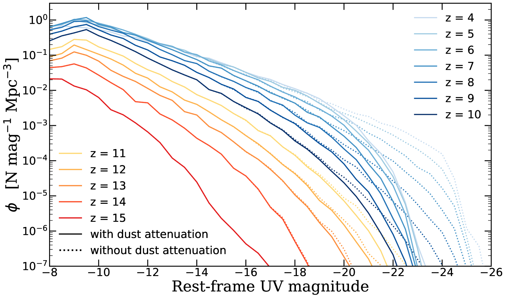
Figure 1: Predicted redshift evolution of the intrinsic (dotted) and dust-attenuated (solid) rest-UV LFs between $z=11$ and 15 (this work; red colour series) and between $z=4$ and 10 (Paper I; blue colour series). The turnover at the faint end is not due to resolution, but rather to the atomic cooling limit. At very high redshifts, the UVLF is not well fit by a Schechter function. At $z\sim 4-8$, the apparent knee in the observed UVLF is largely due to differential dust extinction, which is larger in more luminous galaxies.

The Santa Cruz SAM has been tested extensively in the past and shown to be able to reproduce a wide range of observables. In Paper I, the free parameters were re-calibrated to match a subset of $z\sim 0$ observations after adopting the updated cosmological parameters reported by the Planck Collaboration. We then, in Paper I and Paper II, identified the set of physical prescriptions (e.g. SF recipes) and physical parameters (e.g. SNe feedback slope) that are required to reproduce the evolution seen in observed galaxy populations up to $z\sim 10$. This is encouraging as it suggests the physical processes that shape the formation of galaxies during reionization may not be so different from those that determine the properties of low-redshift galaxies. Taking advantage of the model’s efficiency, we also quantified the impacts on the predicted galaxy populations from the uncertainties in these model components by conducting controlled experiments where we systematically varied the model parameters. We found that the key process that has strong effects on the rest-frame UV luminosities and physical properties for bright, massive galaxies is the SF efficiency or timescale ($\tau_{\text{*,0}}$, see equation (1) in Paper I), which effectively characterizes the gas depletion time. For faint, low-mass galaxies, the UV LF is most sensitive to the stellar feedback relation slope ($\alpha_{\text{rh}}$, see equation (3) in Paper I), which characterizes the dependence of the mass loading factor of cold gas ejected by stellar feedback on halo circular velocity. Currently there are not strong constraints on the faint-end slope of the UV LFs during EoR, where the predicted number density of faint galaxies across different models can vary by up to $\sim 1.5$ dex.

In the following subsections, we highlight how the main moving parts affecting the total emissivity of ionizing photons are treated in this work.

2.1.1 Galaxy populations at ultrahigh redshifts

In order to quantify the contribution of ionizing photons from galaxies at ultrahigh redshifts ($z\gtrsim 10$), we extend the predictions from our SAM up to $z\sim 15$. To assign a volume-averaged density to these galaxies, we use the same functional form for the HMF with the fitting parameters tuned to fit the results from the same set of simulations (Bolshoi-Planck and Visbal et al., see fig. 14). See Appendix A for full details and the values of all parameters. In fig. 1, we present both the intrinsic (dust-free) and the dust-attenuated rest-frame UV luminosity functions predicted for the extended redshift range $z=11$–15. In the same figure, we also compare these galaxies to the evolution between $z=4$–10 previously presented in Paper I. Tabulated values for the dust-attenuated UV LFs are provided in Appendix B. In Appendix C, we compare the predicted UV LFs at $z=6$, 8, 9, and 10 to the latest observational constraints (obtained well after publication of our models) and find excellent agreement. We emphasize that the turnover at the faint end of our predicted luminosity functions is not due to resolution but is a result of the atomic cooling limit, which corresponds to a limiting halo mass that evolves with redshift. We found in our predictions that the characteristic ‘knee’ in UV LFs vanishes at $z\gtrsim 9$, seemingly due to both insignificant AGN feedback and lacking of dust (see fig.1), and the faint-end slopes also gradually flatten as a function of rest-UV. The Schechter function is no longer a good representation and therefore, we do not provide Schechter fitting parameters.

We continue to explore the impacts from modelling uncertainties in the context of cosmic reionization. In fig. 2, we show UV LFs predictions for $\alpha_{\text{rh}}=2.0$, 2.4, 3.2, and 3.6. This is consistent with the findings in Paper I and Paper II, where we showed that the faint-end slope of the UV LFs is inversely correlated with the stellar feedback parameter $\alpha_{\text{rh}}$ (i.e., a stronger dependence of wind mass loading on halo circular velocity leads to a flatter faint end slope). Furthermore, this effect also effectively shifts the halo occupation function and the turnover in the faint end of the UV LFs, which corresponds to the atomic cooling limit. In other words, we predict that the magnitude where the UF LF is truncated is inversely related with the strength of stellar feedback.

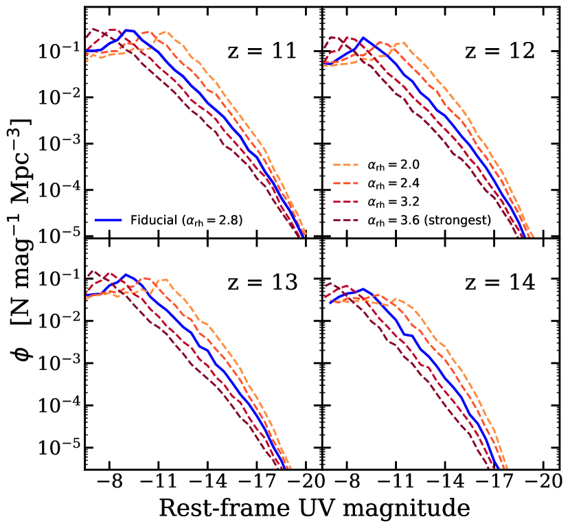
Figure 2: Redshift evolution of the dust-attenuated UV LFs between $z=11$ and 14 predicted by our fiducial model ($\alpha_{\text{rh}}=2.8$, blue solid line). We show four additional scenarios where we vary the parameter controlling the mass-loading of stellar driven winds, with $\alpha_{\text{rh}}=2.0$ (weakest, lightest colour), 2.4, 3.2, and 3.6 (strongest, darkest colour). Larger values of $\alpha_{\text{rh}}$ produce stronger suppression of star formation in low-mass halos, leading to shallower faint end slopes and a lower luminosity for the turnover.

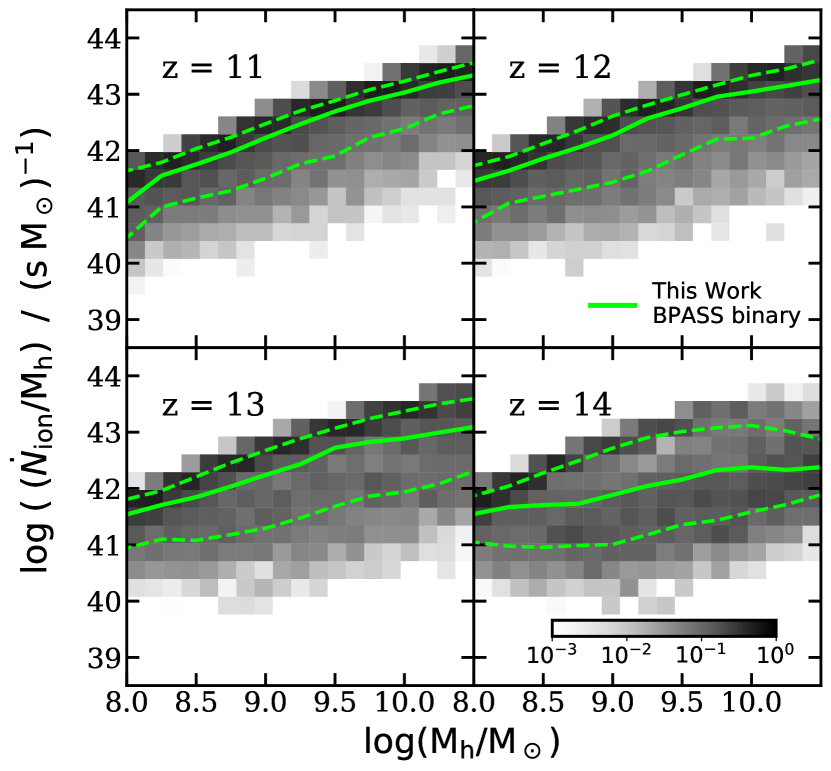
Figure 3: Specific ionizing photon production rate, $\dot{N}_{\text{ion}}/M_{\text{h}}$, as a function of halo mass between $z=11$ and 14, predicted by our fiducial model. The green solid and dashed lines mark the 50th, 16th, and 84th percentiles. The greyscale 2D histograms show the conditional number density per Mpc³ in each bin, normalized to the number density in the corresponding (vertical) halo mass bin. The figure shows a decline in the specific ionizing photon production rate at fixed halo mass with increasing redshift, and a flattening dependence on halo mass. This is because these very early halos have not yet had time to form many stars.

2.1.2 The intrinsic production rate of ionizing radiation

We refer to the ionizing photon production rate, $\dot{N}_{\text{ion}}$, and the production efficiency, $\xi_{\text{ion}}$, by stellar populations in galaxies, which does not account for the absorption or attenuation by the ISM and CGM, as ‘intrinsic’. In Paper III, we self-consistently predict $\dot{N}_{\text{ion}}$ within the Santa Cruz modelling framework, based on the predicted star formation and chemical enrichment histories and results from stellar population synthesis (SPS) models. This model component enables us to distinguish and track the contribution from galaxies across different rest-frame UV magnitudes and stellar masses. In this work, we adopt the published results from the data tables released by the BC03 and the bpass group (Stanway et al., 2016; Eldridge et al., 2017; Stanway & Eldridge, 2018). Both models assume a Chabrier IMF with an upper mass cutoff $m_{\text{U}}=100$M_⊙. These predictions for $z=4$–10 have been examined in detail in Paper III. In that work, we also explored the scaling relations of $\xi_{\text{ion}}$ and $\dot{N}_{\text{ion}}$ with many SF-related physical properties and found that $\xi_{\text{ion}}$ is mildly correlated with $M_{*}$ and SFR, and these scaling relations evolve mildly as a function of redshift (where the underlying driving physical parameter is predominantly stellar metallicity). Although the bpass SPS models account for mass transfer and mergers in stellar binaries, some processes that could potentially boost the production rate of ionizing photons, such as accreting white dwarfs and X-ray binaries, are not included in these models.

Here we extend these predictions to even higher redshift galaxy populations. In Fig. 3, we provide the predictions for the specific ionizing photon production rate, $\dot{N}_{\text{ion}}/M_{\text{h}}$, for halos in a relevant mass range at $z=11$–14. The 2D histograms are shaded according to the conditional number density (Mpc^-1) of galaxies in each bin, which is normalized to the sum of the number density in its corresponding (vertical) halo mass bin. The median, 16th, and 84th percentiles are marked in each panel to illustrate the statistical distribution. Comparing to the predictions between $z=4$ to 10 shown in Fig. 7 in Paper III, which showed $\dot{N}_{\text{ion}}/M_{\text{h}}$ increases across the halo mass range explored, we find that the production rate per halo mass seem to have plateaued has noticeably larger scatter.

2.1.3 Escape fraction of Lyman-continuum photons

The LyC escape fraction can be very stochastic depending on the many intricate physical processes occurring in individual galaxies and their internal structure. In this work, we take a simplistic approach and regard it as a population-averaged quantity, which can either be understood as the population of galaxies all sharing the same escape fraction or as the escape fraction of the total number of ionizing photons collectively produced by all galaxies. We treat it as a controlled free parameter, which may either be a constant value or evolve as a function of redshift. For the remainder of this work, we refer to the LyC escape fraction as $f_{\text{esc}}$.

Inspired by the functional form presented by Kuhlen & Faucher-Giguère (2012), we adopt the following expression for the redshift-evolution of $f_{\text{esc}}$:

$$f_{\text{esc}}(z)=\frac{f_{\text{esc,max}}}{1+\left(\frac{f_{\text{esc,max}}}{f_{\text{esc,0}}}-1\right)\;e^{-k_{0}(z-z_{0})}}\text{,}$$ (1)

assuming $f_{\text{esc}}$ decreases from some maximum value at high redshift, $f_{\text{esc,max}}$, at a characteristic growth rate, $k_{0}$, until it asymptotically reaches an anchoring valuing $f_{\text{esc,0}}$ at a given redshift $z_{0}=4$. A goal of this work is to obtain constraints on $f_{\text{esc}}$ under this empirical parametrization, as required by the set of currently available observational constraints.

2.2 Analytic model for reionization history

In this section, we present the set of analytic equations that tracks the reionization history of intergalactic hydrogen under the influence of the predicted galaxy populations. The model used in this work is similar to the ones presented in Madau et al. (1999, see also ), modified to fully utilize the predictions from the Santa Cruz SAM for galaxy formation. With this model, we can efficiently predict volume-averaged ionizing photon emissivity ($\dot{n}_{\text{ion}}$), IGM ionized fraction ($Q_{\text{\text{H\,{ii}}}}$), and the Thompson scattering optical depth ($\tau_{\text{CMB}}$). In conjunction with the Santa Cruz SAM, the full modelling pipeline effectively connects the ‘ground-level’ galaxy formation physics to the ‘top-level’ cosmic reionization-related observables. With this modelling pipeline, we explore and test the impact of individual model components and how they impact the cosmological scale observables. Note that predictions for helium reionization are beyond the scope of this work.

2.2.1 Ionized volume fraction

The temporal evolution of the volume-averaged ionizing volume filling fraction of ionized hydrogen, $Q_{\text{\text{H\,{ii}}}}$, is described by the first-order differential equation

$$\frac{dQ_{\text{\text{H\,{ii}}}}}{dt}=\frac{\dot{n}_{\text{ion}}}{\bar{n}_{\text{H}}}-\frac{Q_{\text{\text{H\,{ii}}}}}{\bar{t}_{\text{rec}}}\text{,}$$ (2)

derived in Madau et al. (1999). The two terms can be interpreted as a growth term and a sink term, respectively, where the former is the ratio of the comoving ionizing emissivity, $\dot{n}_{\text{ion}}$, and the volume-averaged comoving number density for intergalactic hydrogen, $\bar{n}_{\text{H}}$; the latter is characterized by the ionized volume fraction divided by the recombination timescale of ionized hydrogen, $\bar{t}_{\text{rec}}$. We adopted $\bar{n}_{\text{H}}=1.9\times 10^{-7}$ cm^-3 as reported by Madau & Dickinson (2014).

Table 1: Summary of components for reference model.

Model / Constraints	References	Configurations	Remarks
Star formation	Bigiel et al. 2008	two-slope ($1\rightarrow 2$)	adopted as implemented in PST14 and SPT15
Gas partitioning	Gnedin & Kravtsov 2011	metallicity-based	adopted as implemented in PST14 and SPT15
Stellar feedback	Somerville et al. 2008	$\alpha_{\text{rh}}=2.4$, $\varepsilon_{\text{SN}}=1.7$	re-calibrated and tested in Paper I and Paper II
LyC productivity	Stanway & Eldridge 2018	binary, v2.2.1	newly implemented and tested in Paper III
H ii recombination	Hui & Gnedin 1997	Case B	adopted as implemented in Finkelstein et al. 2019
H ii clumping factor	Pawlik et al. 2015	L25N512 simulation	adopted as implemented in Finkelstein et al. 2019
Emissivity constraints	Becker & Bolton 2013	$\dot{n}_{\text{ion}}$ at $z=2$–5	derived with cosmology consistent with this work
CMB constraints	Planck Collaboration 2016b	$\tau_{\text{CMB}}=0.058\pm 0.012$	derived with cosmology consistent with this work

2.2.2 Ionizing emissivity

The comoving emissivity of ionizing photons, $\dot{n}_{\text{ion}}$, is the total budget supplied to reionize the IGM by galaxies, which is commonly modelled as the product of cosmic SFR or UV density, the LyC production efficiency of ionizing photons, and the fraction of photons that escapes to the IGM

$$\dot{n}_{\text{ion}}=f_{\text{esc}}\;\xi_{\text{ion}}\;\rho_{\text{UV}}\textit{.}$$ (3)

Recalling that in our models, $f_{\text{esc}}$ and $\xi_{\text{ion}}$ may have a different value for each galaxy, instead of combining these for the whole population as above, we calculate the comoving value at each redshift by summing over all predicted galaxies

$$\dot{n}_{\text{ion}}=\sum\limits_{i}\;n_{\text{h},i}\;\dot{N}_{\text{ion},i}\;f_{\text{esc},i}\text{,}$$ (4)

where $n_{\text{h}}$ is the number density per Mpc³ for each galaxy $i$, assigned based on the virial mass of the host halo (section 2.1.1), $\dot{N}_{\text{ion}}$ is the intrinsic ionizing photon production rate (section 2.1.2), and $f_{\text{esc}}$ is the LyC escape fraction (section 2.1.3). This modified approach does not require a predetermined truncation value of $M_{\text{UV}}$, as the turnover in the galaxy UV LF is a physical feature of our model. Moreover, Fig. 7 of Paper I and Fig. 2 have shown that the magnitude where the UV LF turns over is directly correlated with the faint-end slope, which are both affected by the SN feedback slope $\alpha_{\text{rh}}$. Therefore, instead of exploring a range of LF faint-end slope as is frequently done in other studies, we explore a range of $\alpha_{\text{rh}}$.

2.2.3 Intergalactic H ii recombination timescale

The recombination timescale for intergalactic hydrogen is given by

$$\bar{t}_{\text{rec}}=\left[C_{\text{\text{H\,{ii}}}}\;\alpha_{\text{B}}(T)\;(1+\eta Y/4X)\;\bar{n}_{\text{H}}\;(1+z)^{3}\right]^{-1}\text{,}$$ (5)

where $C_{\text{\text{H\,{ii}}}}$ is a redshift-dependent H ii clumping factor and $\eta=1$ for singly ionized helium at $z>4$. We adopted numerical predictions for the clumping factor from the radiation-hydrodynamical simulation L25N512 by Pawlik, Schaye & Vecchia (2015), which $C_{\text{\text{H\,{ii}}}}$ evolves from $\sim 1.5$ to $\sim 4.8$ between $z\sim 14$ to $\sim 6$. The quantity $\alpha_{B}(T)$ is the temperature-dependent case B recombination coefficient for hydrogen given in Hui & Gnedin (1997), where we adopt $T=2\times 10^{4}$ K for the temperature of the IGM at the mean density; $\bar{n}_{\text{H}}$ is the mean density of hydrogen in the IGM. Under the limitation of this type of model, we assume homogeneous recombination.

2.2.4 Thompson scattering optical depth of the CMB

The reionization history, $Q_{\text{\text{H\,{ii}}}}(z)$, is obtained by solving eqn. 2 using Python tools from scipy.integrate.odeint and astropy.cosmology (Robitaille et al., 2013; Price-Whelan et al., 2018; Virtanen et al., 2020). We can then calculate the Thomson scattering optical depth of the CMB, $\tau_{\text{CMB}}$, using

$$\tau_{\text{CMB}}=\int^{\infty}_{0}dz\frac{c(1+z)^{2}}{H(z)}Q_{\text{\text{H\,{ii}}}}(z)\sigma_{\text{T}}\bar{n}_{\text{H}}(1+\eta Y/4X)\text{,}$$ (6)

where $H(z)$ is the Hubble constant and $\sigma_{\text{T}}$ is the Thomson cross section.

The main components of our default ‘reference model’, used throughout the remainder of this work are summarized in Table 1. This approach provides quick estimates of the volume-averaged reionization history and other cosmological-scale observables. However, it does not track the growth of individual Stromgren spheres. It also does not account for local density variances (e.g. void or over-dense regions), which may significantly affect the reionization histories on small scales. We will further discuss the limitations of the model in section 4.

3 IGM reionization by high-redshift galaxies

In this section, we present a collection of predicted reionization histories and investigate how galaxy formation physics can affect these predictions. We experiment with a range of constant values of $f_{\text{esc}}$ (section 3.1) or treat it as a function of redshift (section 3.2). We also present a comparison with two other analogous studies (section 3.3). At the end of the section, we probe the contribution of galaxies from different rest-$M_{\text{UV}}$, as well as forecasting the contribution from galaxies observable by JWST.

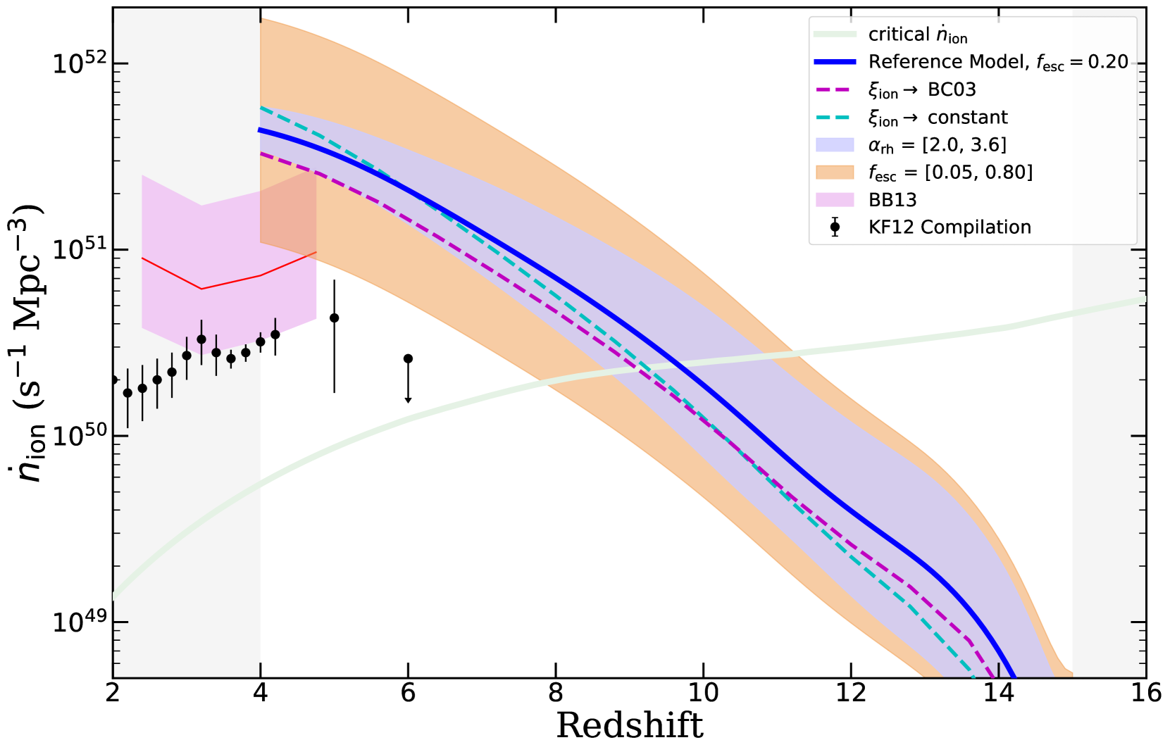
Figure 4: Ionizing photon emissivity, $\dot{n}_{\text{ion}}$, as a function of redshift predicted with the reference model configurations (blue solid, see Table 1). The blue shaded region marks the range of $\dot{n}_{\text{ion}}$ from galaxy populations predicted for $\alpha_{\text{rh}}=2.0$ (weaker feedback, leading to a higher number density of low-mass galaxies and higher emissivity) and 3.6 (stronger feedback, leading to fewer low-mass galaxies and lower emissivity). The orange region marks the range predicted with $f_{\text{esc}}=0.05$ (lower emissivity due to low escape fraction) and 0.80 (higher emissivity). We also include predictions made with a constant $\log(\xi_{\text{ion}})=25.30$ and with $\dot{N}_{\text{ion}}$ from the SPS models of BC03. These results are compared to observational constraints from BB13 and a compilation from KF12. The light green band shows the critical ionizing photon emissivity required to keep the Universe ionized (see eqn. 5 and associated description in text). This shows how uncertainties in different model components could have affected the total ionizing budget throughout the EoR.

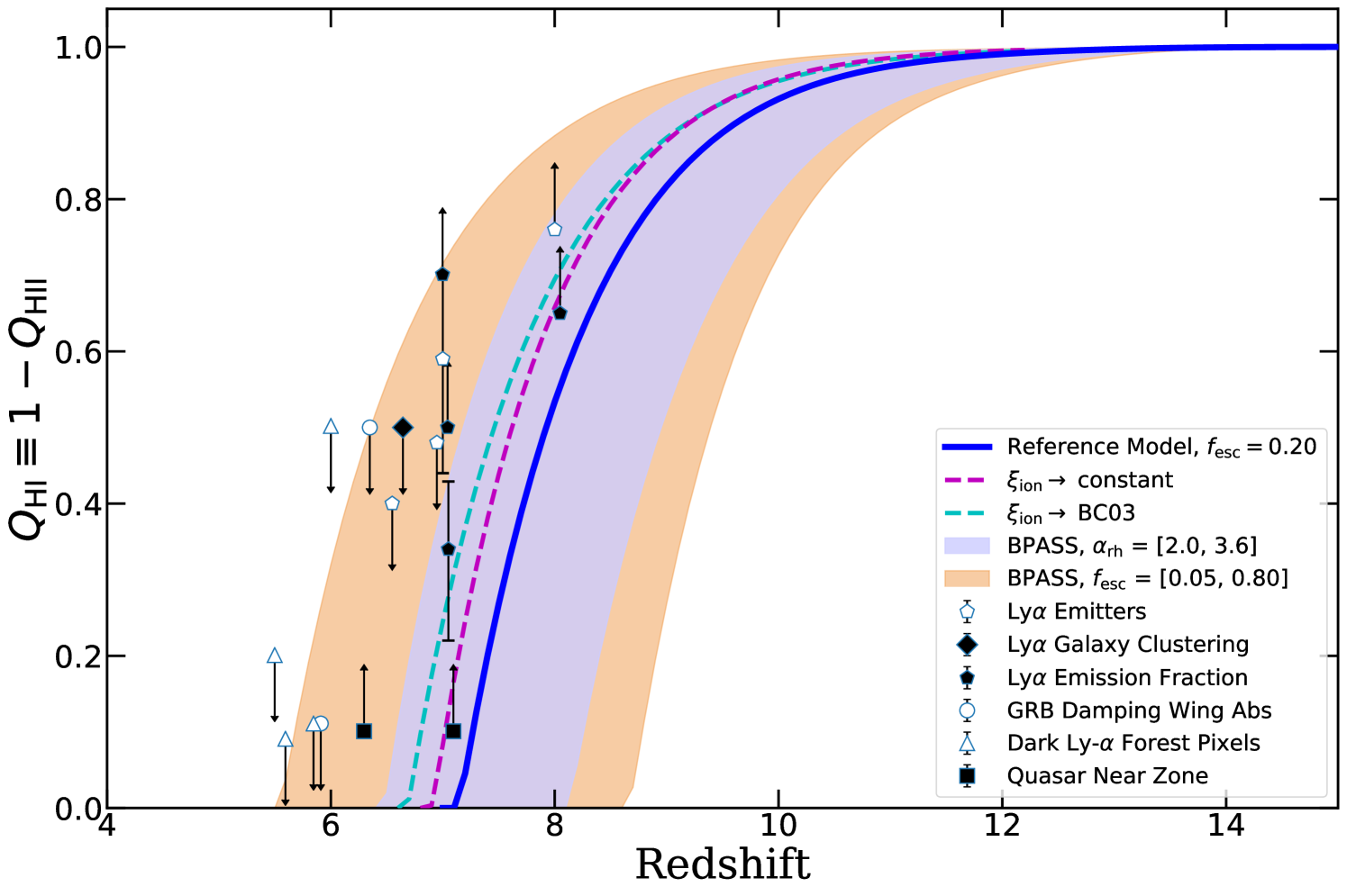
Figure 5: Neutral volume fraction, $Q_{\text{\text{H\,{i}}}}\equiv 1-Q_{\text{\text{H\,{ii}}}}$, as a function of redshift calculated for our reference model (blue solid). The blue shaded region marks the range for galaxy populations predicted for $\alpha_{\text{rh}}=2.0$ (weaker feedback; lower bound) and 3.6 (stronger feedback; upper bound). The orange region marks the range predicted with $f_{\text{esc}}=0.05$ (upper bound) and 0.80 (lower bound). We also include predictions made with a constant $\log(\xi_{\text{ion}})=25.30$ and with $\dot{N}_{\text{ion}}$ from BC03. These results are compared to a compilation of observational constraints from R13 and R15, and additional constraints from Mason et al. (2018a, 2019). The simple reference model, with fixed $f_{\text{esc}}$, is in tension with these observations, though it is clear that this is primarily due to uncertainties on $f_{\text{esc}}$.

3.1 Constant escape fraction

At first, we take the simplest approach by letting $f_{\text{esc}}$ be a non-evolving, universal quantity. We present predictions for $\dot{n}_{\text{ion}}$, $Q_{\text{\text{H\,{ii}}}}$, and $\tau_{\text{CMB}}$ using our reference model configurations. Taking advantage of the efficiency of our modelling pipeline, we then performed a controlled experiment by varying a set of selected model components to quantity their impact on these predictions.

In Fig. 4, we show the evolution of $\dot{n}_{\text{ion}}$ predicted by the reference model assuming $f_{\text{esc}}=0.20$. These results are compared to constraints on the global LyC emissivity at $2<z<5$ derived from the high-redshift Ly$\alpha$ forest by BB13. The plotted data are for the fiducial temperature-density parameter $\gamma=1.4$ and spectral index of the ionizing sources $\alpha=2.0$, with shaded area showing the reported total error. Historically, there has been tension between the Thomson scattering optical depth of the CMB, $\tau_{\text{CMB}}$ and the ionizing photon emissivity at intermediate redshift, as discussed in the introduction. To demonstrate how these new constraints have eased the tension, we also show the compilation of constraints presented in Kuhlen & Faucher-Giguère (2012), which includes Ly$\alpha$ forest observations from Bolton & Haehnelt (2007); Faucher-Giguère et al. (2008b); Prochaska et al. (2009); Songaila & Cowie (2010). The BB13 constraints are a factor of $\sim 2$ higher than the previous measurements, and no longer require the total LyC emissivity to decrease so rapidly at $z\lesssim 6$. We also show the critical comoving ionizing emissivity, $\dot{n}^{\text{crit}}_{\text{ion}}$, or the minimum $\dot{n}_{\text{ion}}$ that is required to keep the Universe ionized

$$\dot{n}^{\text{crit}}_{\text{ion}}=C_{\text{\text{H\,{ii}}}}\;\alpha_{\text{A}}(T)\;(1+\eta Y/4X)\;{\bar{n}_{\text{H}}}^{2}\;(1+z)^{3}\textit{,}$$ (7)

obtained by inverting the recombination timescale given in eqn. 5. Here, the temperature-dependent case A recombination coefficient for hydrogen, $\alpha_{A}(T)$, given by Hui & Gnedin (1997) is invoked because direct recombination from free to the ground bound state is more likely to occur in the optically thin IGM. On the contrary, case B is more suitable at describing regions near a source given that photons released by free-to-ground recombination are likely to reionize a nearby hydrogen atom in these denser regions (see Faucher-Giguère et al. 2009 for an in-depth discussion). The rest of the variables are consistent with the ones adopted in our calculation of the H ii recombination timescale.

We compare these results with alternative scenarios predicted with a range of $f_{\text{esc}}$ and SN feedback slopes $\alpha_{\text{rh}}$. As previously explored in the series, we found that SN feedback is the dominant process that regulates star formation in low-mass halos. Deviating from the fiducial value $\alpha_{\text{rh}}=2.8$, we found that the range $\alpha_{\text{rh}}=2.0$ to 3.6 yield a range of faint-end slopes that are still well within the current observational uncertainties at $z\gtrsim 6$. As shown in Fig. 7 of Paper I and in Fig. 2, low-mass galaxies are more abundant when feedback is weaker ($\alpha_{\text{rh}}=2.0$) and, conversely, less abundant when feedback is stronger ($\alpha_{\text{rh}}=3.6$). Here, we show the range of predicted $\dot{n}_{\text{ion}}$ for galaxy populations predicted with these boundary cases and found that these yield results nearly $\sim 1$ dex apart. Similarly, we also experiment with a wide range of $f_{\text{esc}}=0.05$ to 0.80 to quantify its impact on the overall emissivity. From these results, we can already see that the LyC emissivity is more sensitive to the escape fraction than the faint-end slope of the UV LFs, for these variables within a physically meaningful range.

To explore the uncertainties in modelling $\dot{N}_{\text{ion}}$, we added predictions with $\dot{N}_{\text{ion}}$ from BC03, which is the least optimistic model explored in Paper III, and a scenario with constant $\xi_{\text{ion}}$ adopting the expression from Kuhlen & Faucher-Giguère (2012)

$$\dot{N}_{\text{ion}}=2\times 10^{25}\text{s}^{-1}\left(\frac{L_{\text{UV}}}{\text{erg s}^{-1}\text{Hz}^{-1}}\right)\zeta_{\text{ion}}\text{,}$$ (8)

where $\zeta_{\text{ion}}$ is a free parameter that characterizes the hardness of the spectra. Here we assumed $\zeta_{\text{ion}}=1$ as in the fiducial model of KF12. The rest-UV magnitude is converted using $\log_{10}(L_{\text{UV}}/(\text{erg s}^{-1}\text{Hz}^{-1}))=0.4(51.63-M_{\text{UV}})$. This is equivalent to adopting a constant $\log{\xi_{\text{ion}}}=25.30$. We find that models with $\dot{N}_{\text{ion}}$ computed self-consistently from the SPS models result in a shallower growth in $\dot{n}_{\text{ion}}$ over time comparing to the model with a constant $\xi_{\text{ion}}$. This is likely due to ageing and metal enrichment in the stellar populations in these galaxies, which naturally make the production of ionizing photons less efficient, although the number density of galaxies is growing. However, this effect is insufficient to reproduce the BB13 constraints as the flattening due to changes in $\xi_{\text{ion}}$ is quite subtle, and overall $\dot{n}_{\text{ion}}$ is still largely dominated by the fairly rapid growth of the overall number density of galaxies. On the other hand, results using $\dot{N}_{\text{ion}}$ predicted by different SPS models seems to have evolved quite similarly over time with the expected factor of $\sim 2$ offset due to the inclusion of binary stars in the bpass models. For further discussion of differences between the bpass binary SPS model and BC03, we refer the reader to the discussion associated with Fig. 12 in Paper III.

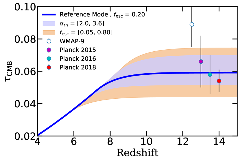
Figure 6: Thomson scattering optical depth of the CMB, $\tau_{\text{CMB}}$, as a function of redshift predicted by our reference model (blue solid). The blue shaded region marks the range of integrated $\tau_{\text{CMB}}$ from galaxy populations predicted for $\alpha_{\text{rh}}=2.0$ (upper bound) and 3.6 (lower bound). The orange region marks the range predicted with $f_{\text{esc}}=0.05$ (lower bound) and 0.80 (upper bound). We also show reported values from the Planck Collaboration 2014; 2016b; 2018 and from WMAP-9 (Hinshaw et al., 2013). Our reference model has no difficulty accounting for the more recent estimates of $\tau_{\text{CMB}}$.

In the same spirit as the $\dot{n}_{\text{ion}}$ comparison, in fig. 5 we present the predicted IGM neutral fraction, $Q_{\text{\text{H\,{i}}}}\equiv 1-Q_{\text{\text{H\,{ii}}}}$, from the same set of model variants. These predictions are stacked up against a compilation of observational constraints compiled from R13 and R15, which consist of various kinds of observations, including Ly$\alpha$ emitting galaxies (Ota et al., 2008; Ouchi et al., 2010; Pentericci et al., 2014; Schenker et al., 2014), Ly$\alpha$ emission fraction (McQuinn et al., 2007; Mesinger & Furlanetto, 2008; Dijkstra et al., 2011), Ly$\alpha$ galaxy clustering (Ouchi et al., 2010), Ly$\alpha$ damping wing (Totani et al., 2006; McQuinn et al., 2008; Chornock et al., 2013), from the near zones of bright quasars (Bolton & Haehnelt, 2007; Bolton et al., 2011; Schroeder et al., 2013), and from dark pixels in Ly$\alpha$ forest measurements (Mesinger, 2010; McGreer et al., 2011, 2015). We refer the reader to Robertson et al. (2013) for a detailed description of these constraints. We also added the latest constraints from Ly$\alpha$ emitting galaxies reported by Mason et al. (2018a, 2019).

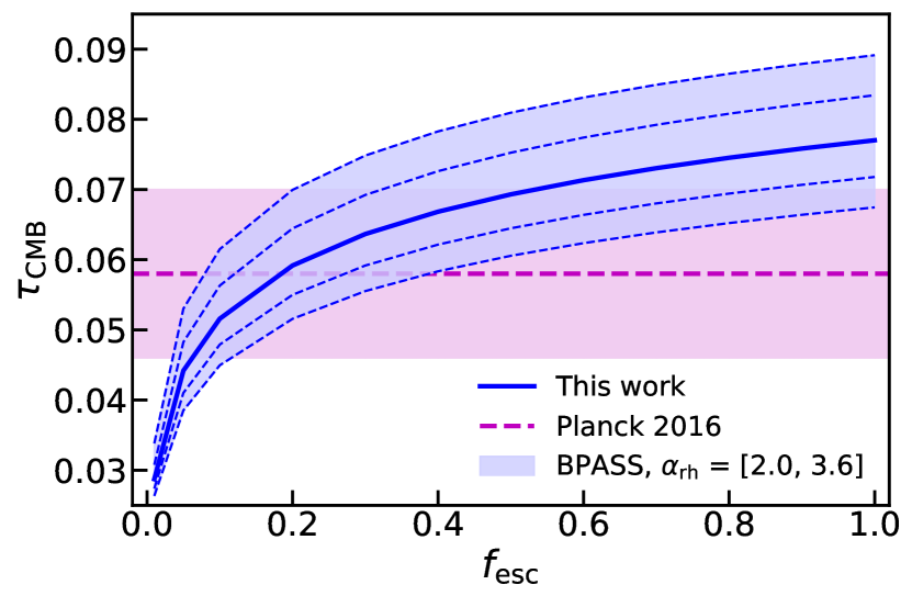
Figure 7: Thomson scattering optical depth of the CMB, $\tau_{\text{CMB}}$, as a function of assumed $f_{\text{esc}}$ and $\alpha_{\text{rh}}$ in our model. Predictions from our reference model are shown by the blue solid line. The blue dashed lines show the alternative predictions made with $\alpha_{\text{rh}}=2.0$ (upper bound for earlier reionization due to higher number density of galaxies), 2.4, 3.2, and 3.6 (lower bound for later reionization due to lower number density of galaxies). The measured value of $\tau_{\text{CMB}}=0.058\pm 0.012$ as reported by Planck Collaboration (2016b) is shown for comparison. This provides a reference showing the interplay between uncertainties or variation in the parameters $f_{\text{esc}}$ and $\alpha_{\text{rh}}=2.0$.

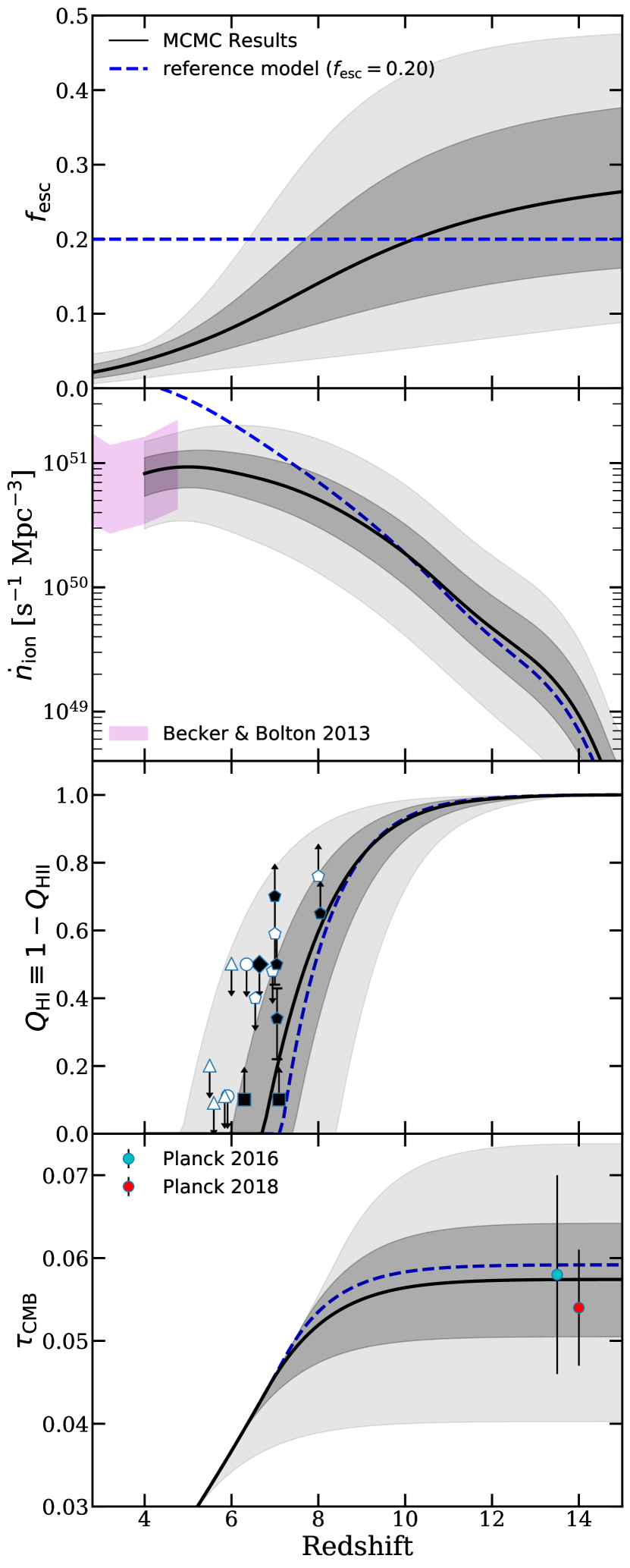
Figure 8: From top to bottom, we show the predicted redshift evolution for $f_{\text{esc}}$, $\dot{n}_{\text{ion}}$, $Q_{\text{\text{H\,{i}}}}$, and $\tau_{\text{CMB}}$ using the BB13 and Planck Collaboration (2016b) $\tau_{\text{CMB}}$ observations as constraints in our MCMC analysis. The shaded areas denote the 68% (dark grey) and 95% (light grey) confidence regions. We also show our reference model with a constant $f_{\text{esc}}=0.20$ for comparison (blue dashed). This figure shows that a moderate effective evolution of $f_{\text{esc}}$ with redshift can comfortably accommodate all of the observational constraints.

Fig. 6 shows $\tau_{\text{CMB}}$ as a function of redshift for our reference model, and for the model variants $f_{\text{esc}}=[0.05,0.80]$ and $\alpha_{\text{rh}}=[2.0,3.6]$. We show recent measurements reported by the Planck Collaboration 2014; 2016b; 2018 and WMAP-9 (Hinshaw et al., 2013). The latest observational constraints together favour both a later conclusion of reionization and a less rapidly evolving $\dot{n}_{\text{ion}}$, which ease both the need for high emissivity at high redshifts and rapid decrease of $\dot{n}_{\text{ion}}$ toward $z\lesssim 5$. In Fig. 7, we show the integrated $\tau_{\text{CMB}}$ as a function of both $f_{\text{esc}}$ and $\alpha_{\text{rh}}$. This shows that $\tau_{\text{CMB}}$ is very sensitive to the LyC escape fraction for $f_{\text{esc}}\lesssim 0.3$, but its dependence on $f_{\text{esc}}$ becomes much flatter above this value. For $f_{\text{esc}}\gtrsim 0.3$, the predicted optical depth is more sensitive to the abundance of faint galaxies rather than the LyC $f_{\text{esc}}$. Note that $\tau_{\text{CMB}}$ is an integrated quantity that compresses the reionization history into a single metric. However, it is degenerately affected by both the conclusion of the phase transition and its progression. For instance, an extremely slow reionization progression or a rapid, late reionization can both result in a lower measured $\tau_{\text{CMB}}$ value.

These results show that models with non-evolving $f_{\text{esc}}$ and $\alpha_{\text{rh}}$ are unable to reproduce a reionization history that simultaneously matches all three sets of constraints, which is consistent with results from previous studies (e.g. Kuhlen & Faucher-Giguère, 2012; Anderson et al., 2017).

3.2 Constraining a redshift dependent escape fraction with MCMC

Results from §3.1 quantified the sensitivity of model outputs to a range of fixed values of $f_{\text{esc}}$ and $\alpha_{\text{rh}}$. In this section, we allow $f_{\text{esc}}$ to evolve as a function of redshift (see eqn.1) and employed a Markov chain Monte Carlo (MCMC) method to find the optimal configuration that is needed to satisfy the current observational constraints. We employ the python MCMC tool emcee by Foreman-Mackey et al. (2013) to survey the four dimensional parameter space, including $f_{\text{esc,max}}$, $f_{\text{esc,0}}$, $k_{0}$, and $\alpha_{\text{rh}}$. In the context of cosmic reionization studied here, we consider the many other free parameters in the galaxy formation model as being collectively constrained either by calibration or by the cross-checks with observations between $z=4$ to 10 in previous works. In this exercise, $\alpha_{\text{rh}}$ can take any value within the range [2.0, 3.6], where $\dot{n}_{\text{ion}}$ is pre-calculated for fixed values of $\alpha_{\text{rh}}=2.0$, 2.4, 2.8, 3.2, and 3.6, and then interpolated using the scipy.interpolate tool. By varying $\alpha_{\text{rh}}$ within the SAM, we have included a number of associated features under its influences, including the faint-end slopes and flattening of the UV LFs, and the subtle boost of ionizing photon production due to the slight increase in burstiness triggered by SN feedback (see section 3.4 and associated discussion in Paper III).

The MCMC framework is set up with 56 walkers, each of which performs a chain of 120,000 steps with the first 200 regarded as burn-in and discarded. Each of these walkers is initialized with a Gaussian distribution, with a chosen peak and half width distribution. The parameters that went into the set-up can be found in Table 2. We assumed a flat prior for all four of our free parameters. For a randomly drawn prior that falls outside the boundary of the flat prior, a new set of parameters are drawn.

Table 2: Summary for the MCMC parameters, flat prior constraints, and posterior with 68% confidence region.

	Initiation	$\sigma$	constraints	posterior
$f_{\text{esc,0}}$	0.036	0.00005	[0.012, 0.060]	$0.0381^{+0.0148}_{-0.0159}$
$f_{\text{esc,max}}$	0.350	0.0005	[0.100, 0.500]	$0.2985^{+0.1357}_{-0.1328}$
$k_{0}$	0.50	0.005	[0.10, 0.90]	$0.523^{+0.255}_{-0.269}$
$\alpha_{\text{rh}}$	2.80	0.05	[2.0, 3.6]	$2.784^{+0.525}_{-0.511}$

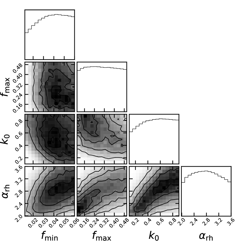
Figure 9: Distributions of the parameter posterior distributions from the MCMC. The parameter $\alpha_{\text{rh}}$ is fairly well constrained, as is the low-redshift (here $z=4$) value of $f_{\text{esc}}$ ($f_{\text{esc,0}}$). The rate of evolution of $f_{\text{esc}}$ ($k_{0}$) and its asymptotic value ($f_{\text{esc,max}}$) are not well constrained. The strong covariance between $\alpha_{\text{rh}}$ and $f_{\text{esc}}$ is apparent.

The set of observational constraints used in the MCMC are the Ly$\alpha$ forest constraints on $\dot{n}_{\text{ion}}$ from BB13 and the $\tau_{\text{CMB}}$ from Planck Collaboration (2016b), which are weighted equally in the likelihood function. Note that the large collection of IGM neutral fraction estimates are shown for comparison but are not used as constraints in the MCMC. The median and the 68% and 95% confidence region of our posteriors for the predicted $f_{\text{esc}}$, $\dot{n}_{\text{ion}}$, $Q_{\text{\text{H\,{i}}}}$, and $\tau_{\text{CMB}}$ are summarized in Fig. 8, where the posterior distributions are shown in Fig. 9.

Our results favour a drop in escape fraction at $z\lesssim 7$, leading to a turn-over in the ionizing emissivity. The parameters $k_{0}$ and $\alpha_{\text{rh}}$ are strongly covariant, and are only weakly constrained by $\tau_{\text{CMB}}$. It is encouraging that the range of predicted reionization histories are in broad agreement with the $Q_{\text{\text{H\,{i}}}}$ constraints. This is non-trivial as it depends on other model components that are not being actively ‘tuned’ here, such as which galaxies are contributing to reionization. We note that the latest Planck Collaboration 2018 result would favour an even milder evolution of $f_{\text{esc}}$ and a slightly lower $f_{\text{esc,max}}$. Adopting the Planck2018 value of $\tau_{\text{CMB}}$ will only mildly change the results and conclusions of this work.

3.3 Comparison with other recent models

In this section, we compare the predicted reionization history in our reference model to recent studies by Finkelstein et al. (2019) and Naidu et al. (2020). In fig. 10, we compare results from our reference model with a constant $f_{\text{esc}}=20\%$ and with the evolving $f_{\text{esc}}$ found in section 3.2 to the results from Finkelstein et al. and Model I (constant $f_{\text{esc}}$) from Naidu et al.. Although these models are fairly similar as they adopted a similar approach to modelling reionization, we note that these works adopted very different approaches to model galaxy populations and their evolution.

Finkelstein et al. use UV LFs from observations with faint-end slopes extrapolated below the current detection limit. These UV LFs are truncated at halo masses corresponding to photoionization squelching and atomic cooling, which are obtained via abundance matching. The many moving parts in the model, including the LyC escape fraction, halo truncation mass, the evolution of $\xi_{\text{ion}}$, and the contribution of AGN, are optimized to fit a set of observational constraints using a MCMC machinery. Finkelstein et al. were particularly interested in exploring models that could satisfy all constraints on reionization while adopting a low ionizing escape fraction ($\lesssim 5$% throughout the EoR). They adopted a halo-mass dependent parametrization of $f_{\text{esc}}$ based on hydrodynamic simulations from Paardekooper et al. (2015), and paramterized $\xi_{\text{ion}}$ in terms of redshift and galaxy luminosity.

On the other hand, Naidu et al. adopted galaxies from the Tacchella et al. (2018) empirical model (see comparison with our predictions in Paper II) and estimated the production efficiency of ionizing photons using synthetic SEDs generated from the Flexible Stellar Population Synthesis (FSPS; Conroy et al., 2009, 2010) and MESA Isochrones and Stellar Tracks (MIST; Choi et al., 2017) for individual galaxies. They have explored a model with fixed $f_{\text{esc}}$ and one that scales as a function of $\Sigma_{\text{SFR}}$, and a range of truncation values $M_{\text{UV}}$.

Finkelstein et al. found that in order for models with such universally low escape fractions to be viable, a rather high and rapidly evolving $\xi_{\text{ion}}$ is required. The range of $\xi_{\text{ion}}$ values are similar to, or even above, the observed values from Bouwens et al. (2016). However, Paper III, Wilkins et al. (2016), and Ceverino et al. (2019) have shown that such high values of $\xi_{\text{ion}}$ and such strong evolution are not ‘naturally’ predicted in current self-consistent galaxy formation models. As we can see in fig. 10, the Finkelstein et al. model (in which reionization is heavily dominated by low-mass galaxies) predicts an early start to reionization and a more gradual evolution for $Q_{\text{\text{H\,{i}}}}$. The Naidu et al. model (in which massive galaxies play a more important role) predicts later and more rapid reionization. Curiously, our model lies somewhere in between, although it also predicts a fairly rapid transition in $Q_{\text{\text{H\,{i}}}}$.

This comparison illustrates that there is still significant uncertainty in which galaxies dominate the reionization of the Universe and the details of how reionization progressed. Future observations JWST and other facilities will provide direct constraints on the source populations (as we explore further in the next section). Furthermore, as galaxies of different masses cluster very differently in space, these models would also have very different implications for the topology of reionization, which will eventually be probed with 21-cm intensity mapping experiments.

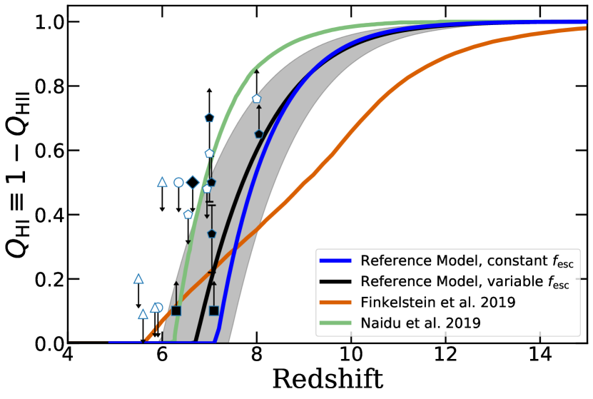
Figure 10: The redshift evolution of the IGM neutral fraction predicted by our reference model with a constant $20\%$ (blue) escape fraction, and our fiducial model with an evolving (black line and shaded regions) escape fraction, compared to predictions from the recent models of Finkelstein et al. (2019) (orange) and Naidu et al. (2020) (green). A compilation of observational constraints is shown by the symbols (see Fig. 5 for a legend). This illustrates the broad range of reionization histories implied by several of the most recent modeling papers.

3.4 Which galaxies reionized the Universe and will JWST see them?

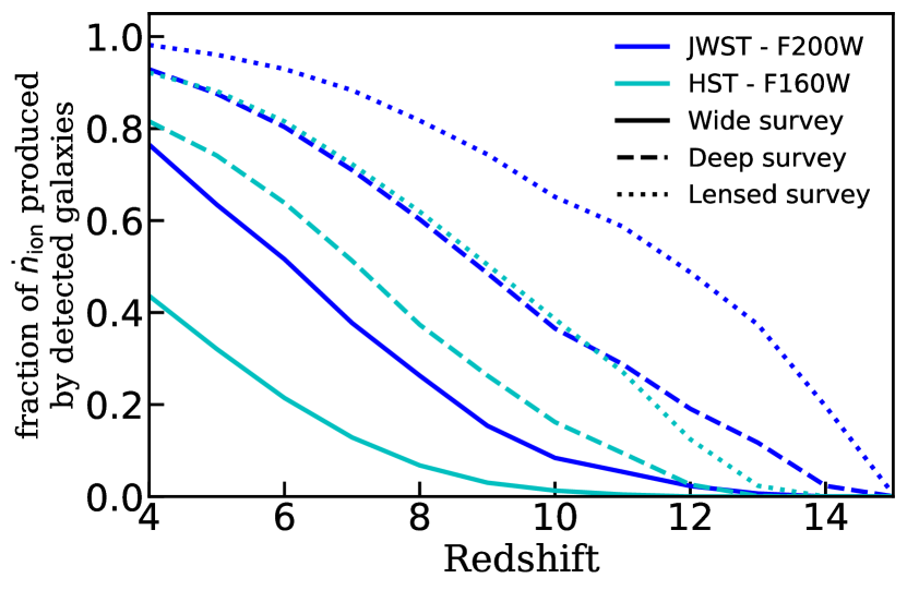
Figure 11: Predictions from our reference model for the fraction of ionizing photons produced by galaxies that are expected to be detected in various types of surveys, including wide (solid), deep (dashed), and lensed (dotted) surveys with JWST (blue) and HST (cyan) between $z=4$ and 15. Survey areas and detection limits assumed for these calculations are detailed in the text. These predictions reflect the production rate and do not account for the escape fraction of ionizing photons possibly varying across galaxies with different luminosities.

In this section, we take advantage of the completeness of our predictions both in mass and redshift to estimate the contributions of ionizing photons from galaxies of different intrinsic luminosities, and estimate what fraction of the ionizing photon budget will be contributed by galaxies that are anticipated to be observed in future JWST surveys. We show predictions for our reference model. As the dependence of $f_{\text{esc}}$ on galaxy luminosity is very uncertain, and not yet included in our modelling, we only provide predictions here for the fraction of ionizing photons produced and do not try to estimate the fraction that escape to the IGM. Recent simulation works have shown that $f_{\text{esc}}$ may inversely scale with $M_{\text{h}}$ in a fairly loose way (e.g. Paardekooper et al., 2015), and therefore the actual contribution from massive/luminous galaxies to the overall ionizing photon budget might be smaller than what is presented here. However, our models do incorporate a mass and redshift dependent $\xi_{\text{ion}}$ based on our self-consistent modelling. These calculations do not account for field-to-field variance nor the survey area, where rare, massive objects may be missing from the small survey area of deep surveys.

In fig. 11, we show the fraction of $\dot{n}_{\text{ion}}$ produced by galaxies above the detection limits of hypothetical JWST wide, deep, and lensed surveys with detection limits of $m_{\text{F200W}}=28.6$, 31.5, and 34.0, respectively. See Table 6 in Paper I and Table 1 in Paper II for detailed configurations of these hypothetical surveys. For comparison, we also show results for legacy HST surveys, where we adopted detection limits for the F160W filter $m_{\text{F160W}}=26.8$, 29.5, and 31.5 for wide, deep, and lensed surveys, respectively, with configurations similar to the CANDELS and Hubble Frontier Fields surveys. At $z\sim 7$–8, where we predict the Universe to be about 50% reionized by volume, JWST will be able to detect the sources of 60-70% of the reionizing photons in a deep survey. This fraction increases to $\sim 90\%$ for an ultra-deep lensed survey, however, interpreting lensed observations and estimating the survey completeness may be more challenging.

In a similar experiment, we break down the galaxy populations by rest-frame intrinsic UV magnitude (not accounting for the effect of dust attenuation) into the following groups: $-24<M_{\text{UV}}<-20$, $-20<M_{\text{UV}}<-16$, $-16<M_{\text{UV}}<-12$, to the faintest $-12<M_{\text{UV}}<-8$. In fig. 12, we compare the fraction of $\dot{n}_{\text{ion}}$ contributed by galaxies from each of these groups from $z=15$ to 4. Galaxies beyond this range combined produce $<1\%$ of ionizing photons across all redshifts, and are omitted here. Similar to results presented in the previous figure, we assume that $f_{\text{esc}}$ does not depend on galaxy properties, which may significantly effect the predictions shown here. We find that ultra-faint galaxies ($-12<M_{\text{UV}}<-8$) dominate at the highest redshifts ($z\gtrsim 13$), with a slightly brighter population $-16<M_{\text{UV}}<-12$ dominating over the redshift range $10\lesssim z\lesssim 13$. At lower redshift $z\lesssim 10$, galaxies in the intermediate luminosity range $-20<M_{\text{UV}}<-16$ dominate.

Similarly, in fig. 13 we break down the contribution of ionizing photons by the host halo masses of galaxies. These are based on the predictions from our reference model configurations, and are quite sensitive to the details of how galaxies populate halos, which as we have shown depends on the details of the stellar feedback parameters and other physical processes. We find that contributions from halos outside the range shown here are insignificant. This result is also useful for estimating the ‘completeness’ of the predicted ionizing emissivity from studies with limited mass resolution. In Paper I (see section 2.2 and fig. 3), we explored the impact on star formation from a photoionizing background using a redshift-dependent characteristic mass approach as described by Okamoto et al. (2008) and found nearly no impact on the galaxy populations at the range of redshift and halo mass relevant to our study. However, high-resolution hydrodynamic simulations have shown that the presence of such a background may have affected the low-mass, ‘photosensitive’ halos of $\log(M_{\text{h}})\lesssim 9$ (Finlator et al., 2013). Accounting for this effect may reduce the contribution from low-mass halos near the beginning of the EoR relative to our predictions.

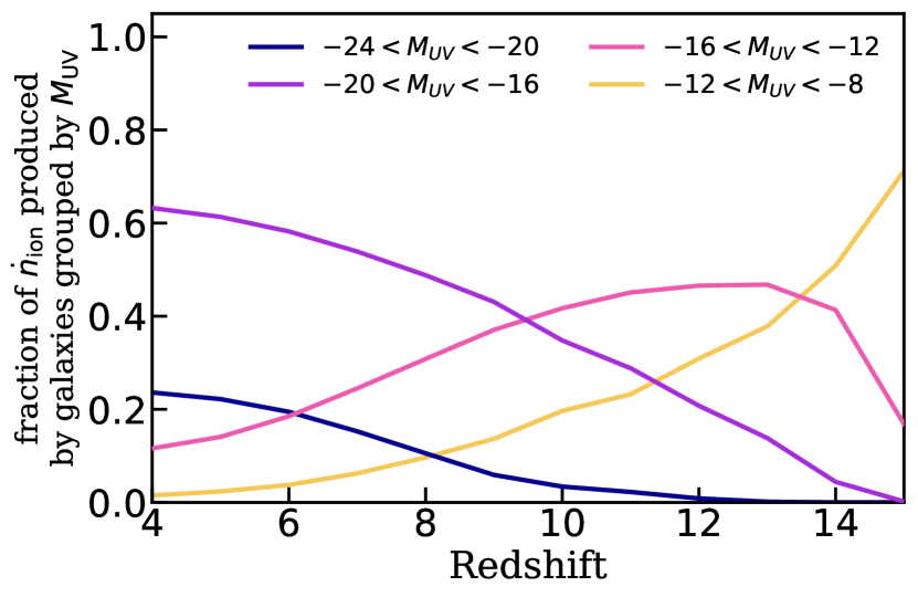
Figure 12: Predictions from our reference model for the fraction of ionizing photons produced by galaxies grouped by rest-frame dust-attenuated $M_{\text{UV}}$ between $z=4$ and 15. These predictions reflect the production rate and do not account for the escape fraction of ionizing photons possibly varying across galaxies with different luminosities. Galaxies outside the range of $M_{\text{UV}}$ shown contribute $<1\%$ of ionizing photons at all times.

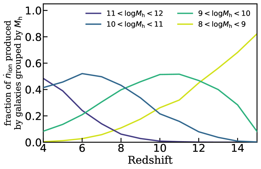
Figure 13: Predictions from our reference model for the fraction of ionizing photons produced by galaxies grouped by host halo mass $M_{\text{h}}$ between $z=4$ and 15. These predictions reflect the production rate and do not account for the escape fraction of ionizing photons possibly varying across halo mass. The contribution of ionizing photons that originates in halos outside the range shown is insignificant.

4 Discussion

In this section, we discuss some caveats and uncertainties in our modelling pipeline, and present an outlook for future observations with JWST and beyond.

4.1 Galaxies forming at extreme redshifts and their role in cosmological events

In this series of papers, we have explored the interplay between galaxy formation physics and the cosmological-scale phase transition of hydrogen reionization. In particular, we investigated whether models with physical recipes and parameters that have been calibrated to match lower redshift observations ($z\sim 0$) are consistent with a broad suite of observations at extremely high redshifts ($z\gtrsim 6$). A significant finding of this work is that these locally calibrated models are consistent (within the uncertainties) with all currently available observations at $z\gtrsim 6$, including direct observations of galaxies, and indirect probes of the reionization history from observations of the IGM and CMB. This has two important implications: 1) It seems that the physical processes regulating star formation and stellar feedback do not operate in a vastly different manner at extremely high redshift. Given our lack of detailed understanding of how these processes work even in the local Universe, this is far from a trivial conclusion. 2) Contrary to some previous suggestions in the literature, the current suite of observations do not require an additional ‘exotic’ population of reionizing sources (other than galaxies, e.g. mini-quasars, Pop III stars, self-annihilating dark matter, etc.) in the early Universe. The remaining uncertainties on several components of our modelling mean that we do not rule out the existence of such sources at some level – but they are not required to satisfy existing constraints.

The overall ionizing photon budget available during the EoR is degenerately affected by physical processes that operate over a vast range of scales. As illustrated in fig. 4, each of these seemingly degenerate components can evolve differently and be constrained independently. In Paper I and Paper II, we provided physically motivated predictions for the evolution of the number density of galaxies at high redshift, which will be further constrained with future galaxy surveys; and in Paper III, we predicted the evolution and distribution of $\xi_{\text{ion}}$ for the same set of galaxies, which may also be constrained with future observations as discussed in Paper III. We have explicitly broken down the contribution to the ionizing photon budget as a function of redshift from galaxies with different observed frame and rest-frame luminosity, and different halo mass. This is again a non-trivial calculation, as the intrinsic production efficiency of ionizing photons depends on a combination of factors such as stellar population age and metallicity in addition to the number density of galaxies with different luminosities. These effects are self-consistently included in our models.

We took a fully semi-analytic approach to assemble our modelling pipeline, including the construction of merger trees, formation and evolution of galaxies, and the progression of cosmic reionization. In practice, this modelling pipeline serves as a low-computational-cost platform for examining galaxy formation and cosmic reionization constraints from various tracers. As shown in fig. 8, the set of IGM neutral fraction constraints seem to collectively favour a relatively rapid decline of neutral hydrogen around $z\sim 6$–7. However, such a reionization history would yield a $\tau_{\text{CMB}}$ near the lower-bound of the reported uncertainties of the latest measurements. Although these constraints are in mild tension, our model is in agreement with all constraints within the 68% confidence regions of the MCMC posterior. Adopting the even lower $\tau_{\text{CMB}}$ measurement reported by the Planck Collaboration in 2018 would further ease this tension and yield a slightly milder evolution for $f_{\text{esc}}$ and a slightly more gradual reionization history.

Another novel aspect of our work is the rigorous statistical exploration of the degeneracy in the physical parameter controlling the impact of stellar feedback on low-mass halos ($\alpha_{\text{rh}}$) and the parametrized effective redshift evolution of $f_{\text{esc}}$. Larger values of $\alpha_{\text{rh}}$ result in stronger feedback, producing fewer low-mass galaxies, and require higher values of $f_{\text{esc}}$ to produce the required budget of ionizing photons, and vice versa. Under the subset of observational constraints included in the MCMC, it is encouraging that the median of the posterior of $\alpha_{\text{rh}}$ is very much in agreement with the value that is required to reproduce $z\sim 0$ observations. Similarly, the required redshift evolution in $f_{\text{esc}}$ is not extreme, and the values at the lower end of our explored redshift range ($z\sim 4$) where there are some observational constraints are reasonable.

Past studies predicted diverging scenarios for the final stage of reionization depending on the assumptions and observational constraints employed by these models. Such process could be rather extended when dominated by low-mass galaxies (e.g. Finkelstein et al., 2019), or conversely very rapid when dominated by massive galaxies (e.g. Mason et al. 2018a and Naidu et al. 2020), for which the rapid end to reionization is motivated by Ly$\alpha$ emitter constraints. The results presented in this work depict a relatively early onset of reionization compared to Naidu et al. due to the early contributions from low-mass galaxies, but lag behind Finkelstein et al. because of the lower predicted $\xi_{\text{ion}}$ and $f_{\text{esc}}$. However, it is very intriguing to see that our model also predicted a very rapid end to reionization when Ly$\alpha$ emitters are not explicitly used to constrain our model. Fig. 12 shows that the contribution of ionizing photons from more massive galaxies has grown rapidly and took over from their low-mass counterparts during the EoR, which provides a physical explanation to the rapid conclusion of reionization that is solely driven by galaxy formation physics rather than from observed EoR constraints.

However, Finkelstein et al. also showed that by letting all galaxies to have the same escape fraction, galaxies with $M_{\text{UV}}\lesssim-16$ would have dominated the ionizing photon budget. Given that the way $f_{\text{esc}}$ is parametrized in this work, it is also possible that we have overestimated the contribution from massive galaxies, which could be a partial reason to the rapid end. Therefore, the predicted rapid end to reionization can be one part backtracked to the predicted evolution of galaxy populations and their spectroscopic properties, and one part due to our parametrization of $f_{\text{esc}}$.

4.2 Caveats, limitations, and uncertainties of the modelling framework

The limitations and caveats regarding the galaxy formation model and the physical recipe for $\dot{N}_{\text{ion}}$ have been thoroughly discussed in previous works; we refer the reader to section 6.3 in Paper II and section 4.3 in Paper III. This discussion will be focused mainly on the topics related to the reionization pipeline presented in this work.

We note that even though the SAM is fairly successful at reproducing a wide variety of existing observational constraints, which we examined in detail in Paper I and Paper II, both the physical properties and number density of the predicted galaxy populations at $z>10$ are poorly constrained due to the lack of direct observations. They are subject to uncertainties in model components, such as feedback effects and SF relations, which are either untested or known to be inaccurate in extreme (e.g. metal-free) environments. There are also missing physical processes, such as the formation of Population III stars, that can potentially affect star formation activity in low-mass halos in the early universe.

Therefore, we regard the predictions for $z=11$ to 15, including both the UV LFs and $\dot{N}_{\text{ion}}$/$M_{h}$, to be more uncertain. We plan to explore the physics relevant to these extreme epochs in future works. In addition, the models will be tested more stringently as high-redshift observational constraints from JWST and other instruments become available.

Furthermore, the EPS-based merger trees adopted in this work series have been compared trees extracted from numerical simulations and the results shown to be in good agreement. However, the EPS algorithm has never been tested over the full halo mass and redshift ranges that are explored in this work, as there is currently no publicly available relevant suite of dark matter only simulations. We plan on running and analysing this suite of N-body simulations, and developing and validating a new and improved fast merger tree algorithm, in Yung et al. (in prep).

Our analytic reionization model does not account for density fluctuations and clustering of sources across the Universe, which numerical simulations have shown can lead to an inhomogeneous and ‘patchy’ progression of reionization. Furthermore, our models do not self-consistently account for photo-ionization feedback (or ‘squelching’). Other works have shown (Gnedin, 2014; Mutch et al., 2016) that photo-ionization affects only galaxies in extremely low mass halos, which we found have a negligible contribution to reionization. Furthermore, post-reionization IGM temperature fluctuation can also be used to constrain the reionization history and this has been explored analytically (Furlanetto & Oh, 2009) and with fully coupled radiation-hydrodynamic simulations (Wu et al., 2019).

Some sources that could be potential contributors to the total ionizing photon budget are not accounted for in this work. These include Population III stars, X-ray binaries, and AGN. Previous work has shown that Pop III stars are unlikely to dominate the reionizing photon budget (e.g. Ricotti & Ostriker, 2004; Greif & Bromm, 2006; Ahn et al., 2012; Paardekooper et al., 2013; Robertson et al., 2015), but they could make reionization more patchy, and are presumably important for polluting early halos with metals, which can then provide the seeds for dust and molecular hydrogen formation. This process is a critical component in our models, which is currently treated in a simplified way by adopting a metallicity ‘floor’ in all pristine halos. We further assume that significant cooling cannot occur in halos below the atomic cooling limit ($10^{4}$ K). While some cooling may occur at lower temperatures due to molecular hydrogen cooling or metal cooling, these are thought to be sub-dominant (Yoshida et al., 2004; Maio et al., 2010; Johnson et al., 2013; Wise et al., 2014; Xu et al., 2016; Jaacks et al., 2018). The contribution of early accreting black holes to reionization remains very uncertain, and we plan to investigate this in upcoming work. In addition to directly contributing ionizing photons through their hard spectrum, semi-analytic calculations have shown that X-rays produced by AGN can boost $f_{\text{esc}}$ (Benson et al., 2013; Seiler et al., 2018). However, hydrodynamic simulations have shown that this effect is not significant (Trebitsch et al., 2018). We also note that the contribution from AGN to the total ionizing photon budget can become fairly significant near the completion of H i reionization (e.g. Dayal et al., 2020), and our results matching the BB13 emissivity constraints may imply an over-prediction of the contribution from galaxies.

Another caveat related to the observational constraints is that the estimates of $\tau_{\text{CMB}}$ are highly covariant with other cosmological parameters, and are derived assuming a simple instantaneous reionization model. As additional constraints on $Q_{\text{\text{H\,{i}}}}$ and the ionizing photon emissivity are obtained, and we gain a better understanding of the uncertainties on these measurements, these could be incorporated as additional constraints in a fitting procedure.

4.3 Constraining galaxy formation during the EoR with JWST and beyond

With both deep- and lensed-field NIRCam surveys anticipated to reach unprecedented detection limits, the extremely sensitive JWST is expected to directly detect and constrain the number density of faint galaxies up to $z\sim 10$. Furthermore, MIRI and NIRSpec will provide high-resolution spectroscopic follow-ups for the spectral features of these galaxies, which will put more robust constraints on $\xi_{\text{ion}}$ and $f_{\text{esc}}$. These measurements will allow us to further test and refine galaxy formation models and to understand the physics that shapes galaxy properties at ultra-high redshift.

The coming decades promise great opportunities for further exploring the high-redshift Universe. The line-up of flagship instruments, include space-based Euclid (Racca et al., 2016) and Wide-Field Infrared Survey Telescope (WFIRST, Spergel et al., 2015), as well as the ground-based Large Synoptic Survey Telescope (LSST, LSST Science Collaboration, 2017). These facilities are capable of surveying large areas, which is complementary to the small field-of-view of JWST. Furthermore, next generation facilities European Extremely Large Telescope (ELT, Gilmozzi & Spyromilio, 2007), Thirty Meter Telescope (TMT, Sanders, 2013), and Giant Magellan Telescope (GMT, Johns, 2008) have the capability of doing spectroscopic follow-up on the expected large number of photometric detections. The flexibility of our model allows it to be easily adapted to made predictions for these instruments, and facilitate physical interpretation for future multi-instrument surveys. In addition, the Atacama Large Millimeter Array (ALMA) has the capability of detecting dust continuum as well as fine structure lines such as [CII] and [OII] of $z>6$ galaxies. With the extended modelling framework presented in (Popping et al., 2019) coupled with our SAMs, we will also be able to make predictions for joint JWST–ALMA multi-tracer surveys.

Intensity mapping is a complementary approach that surveys large areas of the sky at relatively coarse angular resolution, potentially providing direct constraints on the conditions of the intergalactic hydrogen and indirect, collective constraints on high-redshift galaxy populations (Visbal & Loeb, 2010; Visbal et al., 2011; Kovetz et al., 2017). Numerous intensity mapping experiments for H i, CO, C ii, and Ly$\alpha$ are planned or underway, including BINGO (Battye et al., 2013), CHIME (Bandura et al., 2014), EXCLAIM (Padmanabhan, 2019), HERA (DeBoer et al., 2017), HIRAX (Newburgh et al., 2016), Tianlai (Chen, 2012), LOFAR (Patil et al., 2017), MeerKat (Pourtsidou, 2016; Santos et al., 2017), CONCERTO (Serra, Doré & Lagache, 2016), PAPER (Parsons et al., 2010), etc., which together pave the way to future large-scale multi-tracer intensity mapping surveys. These observations can also be cross-correlated with galaxy surveys for a comprehensive view of the interaction between galaxies and the cosmic environment. The modelling framework presented here can also provide a powerful tool for efficiently producing physically self-consistent, multi-tracer predictions for intensity mapping experiments (Yang et al. in prep).

Finally, improving radiative hydrodynamic simulations of early galaxy evolution (e.g. Finlator et al., 2018; Wu et al., 2019) will complement our approach by providing more physically motivated priors for our key physical parameters, and suggesting new parametrizations that connect quantities such as escape fraction to galaxy properties (e.g. Seiler et al., 2019) rather than redshift, as we have assumed here. Our approach provides a framework to bridge these detailed self-consistent models with upcoming deep and wide surveys to optimally constrain the physics of early galaxy formation.

5 Summary and Conclusions

In this work, we constructed a physically motivated, source-driven semi-analytic modelling pipeline that links galaxy formation to the subsequent reionization history using an analytic model for reionization. The galaxy formation model has been tested extensively and shown to match extremely well with observational constraints up to $z\sim 10$ in previous works, and we extended these predictions up to $z\sim 15$. We have calculated $\dot{N}_{\text{ion}}$ self-consistently, accounting for the stellar age and metallicity distribution of the stellar population in each galaxies using state-of-the-art SPS models. We presented predictions for the ionizing emissivity, IGM neutral fraction, and Thomson optical depth to CMB throughout the Epoch of Reionization, and compared these to a wide range of observational constraints. In a controlled experiment, we isolated and quantified the effect of each of the major moving parts in the total ionizing photon budget. We also explored two different scenarios with a constant and a redshift-dependent $f_{\text{esc}}$, and determined the required conditions for the predicted galaxy populations to reionize the Universe in the time frame require by IGM and CMB constraints. We explored the covariance of different model components (including $f_{\text{esc}}$ and the efficiency of stellar feedback) using MCMC.

We summarize our main conclusions below.

1. Using a well-tested physical galaxy formation model, which was calibrated only to $z\sim 0$ observations and has been shown to well-reproduce observed distributions from $z\sim 4$–10, we provide predictions for rest-frame UV luminosity functions and ionizing photon production rate for galaxies up to $z=15$.

2. Adopting a non-evolving escape fraction of $\sim 20\%$, the galaxy population predicted by our model yields sufficient amounts of ionizing radiation to be consistent with constraints from the Thomson optical depth $\tau_{\text{CMB}}$. However, this model is in tension with low-redshift Ly$\alpha$ observations on the IGM neutral fraction and observational constraints on the ionizing emissivity at $2\lesssim z\lesssim 6$.

3. We performed a number of controlled experiments to explore the impacts on the reionization history of varying the three main model components that influence the total ionizing photon budget, including the abundance of low-mass galaxies, intrinsic ionizing photon production rate, and LyC escape fraction. We find that the uncertainty on estimates of the total LyC emissivity is dominated by uncertainties on $f_{\text{esc}}$, with the strength of stellar feedback being the second most important factor.

4. We used MCMC to explore the covariance in these two parameters ($f_{\text{esc}}$ and $\alpha_{\text{rh}}$, which parametrizes the efficiency of stellar feedback in low-mass halos). We parametrized the population averaged $f_{\text{esc}}$ as a function of redshift, and jointly constrained these parameters along with $\alpha_{\text{rh}}$ using constraints from Ly$\alpha$ forest observations and $\tau_{\text{CMB}}$ measurements. We found that a ‘population-averaged’ escape fraction that mildly increases from $\sim 4\%$ to $\sim 29\%$ between $z\sim 4$ to 15 satisfies both constraints.

5. We presented predictions for the fraction of ionizing photons produced by galaxies of different rest-UV luminosity as a function of redshift, and for the fraction of the total ionizing photon budget sourced by galaxy populations that will be observable in upcoming surveys with JWST. At $z\sim 7$–8, where we predict the Universe to be about 50% reionized by volume, we predict that JWST will be able to detect the sources of 60–70% of the reionizing photons in a deep survey, and up to $\sim 90\%$ in an ultra-deep lensed survey.

Data availability

The data underlying this article are available in the Data Product Portal hosted by the Flatiron Institute at https://www.simonsfoundation.org/semi-analytic-forecasts-for-jwst/.

Appendix A HMF fitting parameters for the extended redshift range

We adopted the HMF parametrization from Tinker et al. (2008) with parameters calibrated to the Bolshoi-Planck simulation from the MultiDark suite (Rodríguez-Puebla et al., 2016; Klypin et al., 2016). The comoving number density of halos of mass between $M_{\text{vir}}+dM_{\text{vir}}$ is given by

$$\frac{dn_{\text{h}}}{dM_{\text{vir}}}=f(\sigma)\frac{\rho_{m}}{M^{2}_{\text{vir}}}\left|\frac{d\ln\sigma^{-1}}{d\ln M_{\text{vir}}}\right|\text{,}$$ (9)

where $\rho_{m}$ is the critical matter density in the Universe, $\sigma$ is the amplitude of the perturbations, and $f(\sigma)$ is called the halo multiplicity function, which takes the form of

$$f(\sigma)=A\left[\left(\frac{\sigma}{b}\right)^{-a}\right]e^{-c/a^{2}}\text{,}$$ (10)

where $A$, $a$, $b$, and $c$ are free parameters. In this work, as shown in fig. 14, we recalibrate these parameters to match the HMF constraints between $z=11$ – 15 from the Bolshoi-Planck simulation and from Visbal et al. (2018). These parameters are presented in Table A1.

Table A1: Fitting parameters for $f(\sigma)$ parameters that produces the HMF at $z=11$ – 15 used throughout this work as shown in fig. 14.

$z$	$A$	$a$	$b$	$c$
11	0.1668	0.9823	1.100	1.0938
12	0.1468	0.9823	1.000	1.0938
13	0.1468	0.9823	0.900	1.0938
14	0.1268	0.9823	0.750	1.0938
15	0.1268	0.5523	0.600	1.1238

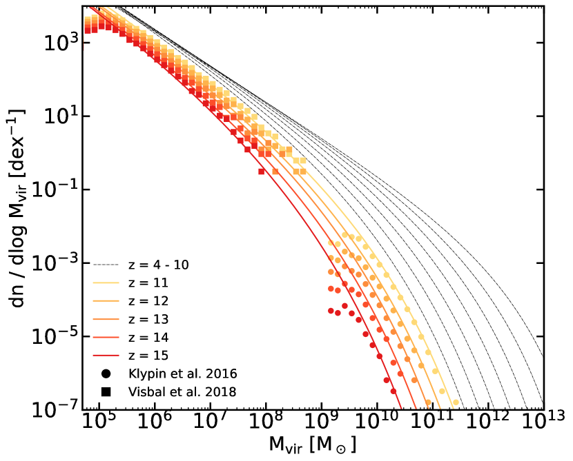
Figure 14: The coloured lines, from light to dark, show the HMF fitting functions adopted for the extended redshift range $z=11$ – 15. $n$-body simulation predictions from Klypin et al. (2016) and Visbal et al. (2018) are shown in matching colour for each redshift for comparison. The light grey dot-dashed lines show HMF fitting functions used for $z=4$ – 10 to guide the eye (see Paper I for detail).

Appendix B Predicted UV Luminosity Functions

Tabulated UV LFs from our fiducial model in the extended redshift range $z=11$ – 15 inducing dust attenuation are presented in Table B1. See online data repository for other data presented in this work.

Table B1: Tabulated UV LFs at $z=11$ – 15 from our fiducial model with dust attenuation as presented in fig. 1 (solid lines).

	$\log_{10}(\phi\,[\text{mag}^{-1}\,\text{Mpc}^{-3}])$
$M_{\text{UV}}$	$z=11$	$z=12$	$z=13$	$z=14$	$z=15$
-22.0	-7.39	-8.36	-10.03	-10.21	-12.18
-21.5	-6.56	-7.51	-8.82	-10.15	-12.04
-21.0	-5.99	-6.79	-7.90	-9.81	-10.82
-20.5	-5.56	-6.31	-7.30	-9.51	-10.33
-20.0	-5.14	-5.83	-6.73	-9.07	-10.08
-19.5	-4.78	-5.41	-6.16	-8.61	-9.16
-19.0	-4.44	-5.13	-5.76	-7.75	-8.85
-18.5	-4.17	-4.70	-5.31	-6.92	-8.50
-18.0	-3.85	-4.37	-4.97	-6.30	-7.91
-17.5	-3.60	-4.11	-4.57	-5.66	-7.53
-17.0	-3.29	-3.80	-4.25	-5.32	-7.05
-16.5	-3.14	-3.52	-3.96	-4.80	-6.63
-16.0	-2.85	-3.29	-3.74	-4.43	-6.36
-15.5	-2.66	-3.03	-3.46	-4.21	-5.98
-15.0	-2.43	-2.84	-3.20	-3.81	-5.64
-14.5	-2.27	-2.61	-3.03	-3.57	-5.20
-14.0	-2.12	-2.40	-2.70	-3.36	-4.61
-13.5	-1.90	-2.28	-2.60	-3.08	-4.19
-13.0	-1.75	-2.04	-2.28	-2.84	-3.92
-12.5	-1.55	-1.90	-2.14	-2.67	-3.49
-12.0	-1.41	-1.65	-1.94	-2.35	-3.18
-11.5	-1.23	-1.51	-1.75	-2.32	-2.92
-11.0	-1.02	-1.28	-1.60	-1.98	-2.70
-10.5	-0.89	-1.11	-1.43	-1.78	-2.55
-10.0	-0.76	-0.97	-1.17	-1.57	-2.20
-9.5	-0.57	-0.84	-1.00	-1.36	-1.98
-9.0	-0.55	-0.71	-0.91	-1.25	-1.88
-8.5	-0.76	-0.95	-1.08	-1.33	-1.68
-8.0	-0.83	-1.05	-1.16	-1.35	-1.67

Appendix C Comparison of Predicted and Observed UV Luminosity Functions

In fig. 15, we compare the predictions of our model to new observational constraints from Atek et al. (2018), Stefanon et al. (2019), and Bouwens et al. (2019), which have been published in the interim since we first published the luminosity function predictions from our models. The models are exactly the same as those published in Paper I. The agreement with the new observations is excellent.

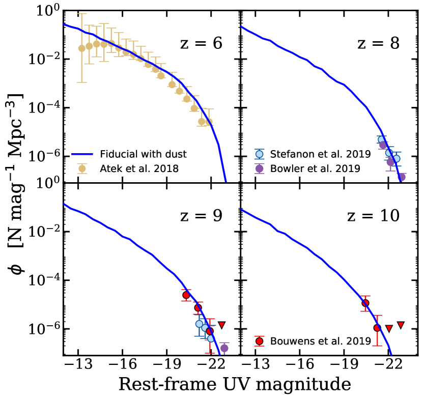
Figure 15: Rest-frame UV LFs from our fiducial model including dust attenuation, reproduced from Paper I and compared to the latest observational constraints from Atek et al. (2018, $z=6$), Stefanon et al. (2019, $z=8$ and 9), Bowler et al. (2020, $z=8$ and 9), and Bouwens et al. (2019, $z=9$ and 10). The agreement with these recent observations is excellent.

References

- Ahn et al. (2012) Ahn K., Iliev I. T., Shapiro P. R., Mellema G., Koda J., Mao Y., 2012, ApJ, 756, L16
- Anderson et al. (2017) Anderson L., Governato F., Karcher M., Quinn T., Wadsley J., 2017, MNRAS, 468, 4077
- Atek et al. (2018) Atek H., Richard J., Kneib J.-P., Schaerer D., 2018, MNRAS, 479, 5184
- Bandura et al. (2014) Bandura K., et al., 2014, Proc. SPIE, 9145, 914522
- Battye et al. (2013) Battye R. A., Browne I. W., Dickinson C., Heron G., Maffei B., Pourtsidou A., 2013, MNRAS, 434, 1239
- Becker & Bolton (2013) Becker G. D., Bolton J. S., 2013, MNRAS, 436, 1023
- Becker et al. (2001) Becker R. H., et al., 2001, AJ, 122, 2850
- Beckwith et al. (2006) Beckwith S. V. W., et al., 2006, AJ, 132, 1729
- Behroozi et al. (2019) Behroozi P., Wechsler R. H., Hearin A. P., Conroy C., 2019, MNRAS, 488, 3143
- Benson et al. (2013) Benson A., Venkatesan A., Shull J. M., 2013, ApJ, 770, 76
- Bigiel et al. (2008) Bigiel F., Leroy A., Walter F., Brinks E., de Blok W. J. G., Madore B., Thornley M. D., 2008, AJ, 136, 2846
- Bolton & Haehnelt (2007) Bolton J. S., Haehnelt M. G., 2007, MNRAS, 382, 325
- Bolton et al. (2011) Bolton J. S., Haehnelt M. G., Warren S. J., Hewett P. C., Mortlock D. J., Venemans B. P., McMahon R. G., Simpson C., 2011, MNRAS, 416, L70
- Bouwens et al. (2011) Bouwens R. J., et al., 2011, ApJ, 737, 90
- Bouwens et al. (2015a) Bouwens R. J., et al., 2015a, ApJ, 803, 34
- Bouwens et al. (2015b) Bouwens R. J., Illingworth G. D., Oesch P. a., Caruana J., Holwerda B., Smit R., Wilkins S., 2015b, ApJ, 811, 140
- Bouwens et al. (2016) Bouwens R. J., Smit R., Labbé I., Franx M., Caruana J., Oesch P., Stefanon M., Rasappu N., 2016, ApJ, 831, 176
- Bouwens et al. (2017) Bouwens R. J., Oesch P. A., Illingworth G. D., Ellis R. S., Stefanon M., 2017, ApJ, 843, 129
- Bouwens et al. (2019) Bouwens R. J., Stefanon M., Oesch P. A., Illingworth G. D., Nanayakkara T., Roberts-Borsani G., Labbé I., Smit R., 2019, ApJ, 880, 25
- Bowler et al. (2020) Bowler R. A. A., Jarvis M. J., Dunlop J. S., McLure R. J., McLeod D. J., Adams N. J., Milvang-Jensen B., McCracken H. J., 2020, MNRAS, 493, 2059
- Boylan-Kolchin et al. (2014) Boylan-Kolchin M., Bullock J. S., Garrison-Kimmel S., 2014, MNRAS, 443, 44
- Boylan-Kolchin et al. (2015) Boylan-Kolchin M., Weisz D. R., Johnson B. D., Bullock J. S., Conroy C., Fitts A., 2015, MNRAS, 453, 1503
- Boylan-Kolchin et al. (2016) Boylan-Kolchin M., Weisz D. R., Bullock J. S., Cooper M. C., 2016, MNRAS, 462, L51
- Bruzual & Charlot (2003) Bruzual G., Charlot S., 2003, MNRAS, 344, 1000
- Carucci & Corasaniti (2019) Carucci I. P., Corasaniti P.-S., 2019, Phys. Rev. D, 99, 023518
- Ceverino et al. (2019) Ceverino D., Klessen R. S., Glover S. C. O., 2019, MNRAS, 484, 1366
- Chen (2012) Chen X., 2012, Int. J. Mod. Phys. Conf. Ser., 12, 256
- Choi et al. (2017) Choi J., Conroy C., Byler N., 2017, ApJ, 838, 159
- Chornock et al. (2013) Chornock R., Berger E., Fox D. B., Lunnan R., Drout M. R., Fong W.-f., Laskar T., Roth K. C., 2013, ApJ, 774, 26
- Choudhury (2009) Choudhury T. R., 2009, Curr. Sci., 97, 841
- Cole et al. (1994) Cole S., Aragon-Salamanca A., Frenk C. S., Navarro J. F., Zepf S. E., 1994, MNRAS, 271, 781
- Conroy (2013) Conroy C., 2013, ARA&A, 51, 393
- Conroy et al. (2009) Conroy C., Gunn J. E., White M., 2009, ApJ, 699, 486
- Conroy et al. (2010) Conroy C., White M., Gunn J. E., 2010, ApJ, 708, 58
- Davé et al. (2019) Davé R., Anglés-Alcázar D., Narayanan D., Li Q., Rafieferantsoa M. H., Appleby S., 2019, MNRAS, 486, 2827
- Dayal & Ferrara (2018) Dayal P., Ferrara A., 2018, Phys. Rep., 780-782, 1
- Dayal et al. (2020) Dayal P., et al., 2020, arXiv:2001.06021
- DeBoer et al. (2017) DeBoer D. R., et al., 2017, PASP, 129, 045001
- Dijkstra et al. (2011) Dijkstra M., Mesinger A., Wyithe J. S. B., 2011, MNRAS, 414, 2139
- Dijkstra et al. (2016) Dijkstra M., Gronke M., Venkatesan A., 2016, ApJ, 828, 71
- Eldridge & Stanway (2009) Eldridge J. J., Stanway E. R., 2009, MNRAS, 400, 1019
- Eldridge et al. (2017) Eldridge J. J., Stanway E. R., Xiao L., McClelland L. A. S., Taylor G., Ng M., Greis S. M. L., Bray J. C., 2017, PASA, 34, e058
- Ellis et al. (2013) Ellis R. S., et al., 2013, ApJ, 763, L7
- Emami et al. (2019) Emami N., Siana B., Alavi A., Gburek T., Freeman W. R., Richard J., Weisz D. R., Stark D. P., 2019, arXiv:1912.06152
- Fan et al. (2006a) Fan X., Carilli C., Keating B., 2006a, ARA&A, 44, 415
- Fan et al. (2006b) Fan X., et al., 2006b, AJ, 132, 117
- Faucher-Giguère et al. (2008a) Faucher-Giguère C.-A., Lidz A., Hernquist L., Zaldarriaga M., 2008a, ApJ, 682, L9
- Faucher-Giguère et al. (2008b) Faucher-Giguère C.-A., Lidz A., Hernquist L., Zaldarriaga M., 2008b, ApJ, 688, 85
- Faucher-Giguère et al. (2009) Faucher-Giguère C.-A., Lidz A., Zaldarriaga M., Hernquist L., 2009, ApJ, 703, 1416
- Feng et al. (2016) Feng Y., Di-Matteo T., Croft R. A., Bird S., Battaglia N., Wilkins S., 2016, MNRAS, 455, 2778
- Finkelstein et al. (2010) Finkelstein S. L., Papovich C., Giavalisco M., Reddy N. A., Ferguson H. C., Koekemoer A. M., Dickinson M., 2010, ApJ, 719, 1250
- Finkelstein et al. (2012) Finkelstein S. L., et al., 2012, ApJ, 758, 93
- Finkelstein et al. (2015) Finkelstein S. L., et al., 2015, ApJ, 810, 71
- Finkelstein et al. (2017) Finkelstein S., et al., 2017, JWST Proposal ID 1345. Cycle 0 Early Release Science
- Finkelstein et al. (2019) Finkelstein S. L., et al., 2019, ApJ, 879, 36
- Finlator et al. (2013) Finlator K., Muñoz J. A., Oppenheimer B. D., Oh S. P., Özel F., Davé R., 2013, MNRAS, 436, 1818
- Finlator et al. (2018) Finlator K., Keating L., Oppenheimer B. D., Davé R., Zackrisson E., 2018, MNRAS, 480, 2628
- Fletcher et al. (2019) Fletcher T. J., Tang M., Robertson B. E., Nakajima K., Ellis R. S., Stark D. P., Inoue A., 2019, ApJ, 878, 87
- Foreman-Mackey et al. (2013) Foreman-Mackey D., Hogg D. W., Lang D., Goodman J., 2013, PASP, 125, 306
- Furlanetto & Oh (2009) Furlanetto S. R., Oh S. P., 2009, ApJ, 701, 94
- Geil et al. (2016) Geil P. M., Mutch S. J., Poole G. B., Angel P. W., Duffy A. R., Mesinger A., Wyithe J. S. B., 2016, MNRAS, 462, 804
- Genel et al. (2014) Genel S., et al., 2014, MNRAS, 445, 175
- Gilmozzi & Spyromilio (2007) Gilmozzi R., Spyromilio J., 2007, The Messenger, 127, 11
- Gnedin (2014) Gnedin N. Y., 2014, ApJ, 793, 29
- Gnedin (2016) Gnedin N. Y., 2016, ApJ, 825, L17
- Gnedin & Kaurov (2014) Gnedin N. Y., Kaurov A. A., 2014, ApJ, 793, 30
- Gnedin & Kravtsov (2011) Gnedin N. Y., Kravtsov A. V., 2011, ApJ, 728, 88
- Gnedin et al. (2017) Gnedin N. Y., Becker G. D., Fan X., 2017, ApJ, 841, 26
- Graus et al. (2016) Graus A. S., Bullock J. S., Boylan-Kolchin M., Weisz D. R., 2016, MNRAS, 456, 477
- Grazian et al. (2017) Grazian A., et al., 2017, A&A, 602, A18
- Greif & Bromm (2006) Greif T. H., Bromm V., 2006, MNRAS, 373, 128
- Grogin et al. (2011) Grogin N. A., et al., 2011, ApJS, 197, 35
- Guaita et al. (2016) Guaita L., et al., 2016, A&A, 587, A133
- Gunn & Peterson (1965) Gunn J. E., Peterson B. A., 1965, ApJ, 142, 1633
- Hassan et al. (2016) Hassan S., Davé R., Finlator K., Santos M. G., 2016, MNRAS, 457, 1550
- Hassan et al. (2017) Hassan S., Davé R., Finlator K., Santos M. G., 2017, MNRAS, 468, 122
- Hinshaw et al. (2013) Hinshaw G., et al., 2013, ApJS, 208, 19
- Hodge et al. (2015) Hodge J. A., Riechers D., Decarli R., Walter F., Carilli C. L., Daddi E., Dannerbauer H., 2015, ApJ, 798, L18
- Hopkins et al. (2014) Hopkins P. F., Kereš D., Oñorbe J., Faucher-Giguère C.-A., Quataert E., Murray N., Bullock J. S., 2014, MNRAS, 445, 581
- Hopkins et al. (2018) Hopkins P. F., et al., 2018, MNRAS, 480, 800
- Hui & Gnedin (1997) Hui L., Gnedin N. Y., 1997, MNRAS, 292, 27
- Iliev et al. (2006a) Iliev I. T., Mellema G., Pen U.-L., Merz H., Shapiro P. R., Alvarez M. A., 2006a, MNRAS, 369, 1625
- Iliev et al. (2006b) Iliev I. T., Mellema G., Pen U.-L., Merz H., Shapiro P. R., Alvarez M. A., 2006b, MNRAS, 372, 679
- Ishigaki et al. (2018) Ishigaki M., Kawamata R., Ouchi M., Oguri M., Shimasaku K., Ono Y., 2018, ApJ, 854, 73
- Jaacks et al. (2018) Jaacks J., Thompson R., Finkelstein S. L., Bromm V., 2018, MNRAS, 475, 4396
- Jiang & van den Bosch (2014) Jiang F., van den Bosch F. C., 2014, MNRAS, 440, 193
- Johns (2008) Johns M., 2008, in Proc. SPIE 6986, Extrem. Large Telesc. Which Wavelengths? Retire. Symp. Arne Ardeb.. p. 698603, doi:10.1117/12.801254
- Johnson et al. (2013) Johnson J. L., Vecchia C. D., Khochfar S., 2013, MNRAS, 428, 1857
- Kamionkowski et al. (1994) Kamionkowski M., Spergel D. N., Sugiyama N., 1994, ApJ, 426, L57
- Kauffmann et al. (1993) Kauffmann G., White S. D. M., Guiderdoni B., 1993, MNRAS, 264, 201
- Kawamata et al. (2016) Kawamata R., Oguri M., Ishigaki M., Shimasaku K., Ouchi M., 2016, ApJ, 819, 114
- Kimm & Cen (2014) Kimm T., Cen R., 2014, ApJ, 788, 121
- Kimm et al. (2017) Kimm T., Katz H., Haehnelt M., Rosdahl J., Devriendt J., Slyz A., 2017, MNRAS, 466, 4826
- Kimm et al. (2019) Kimm T., Blaizot J., Garel T., Michel-Dansac L., Katz H., Rosdahl J., Verhamme A., Haehnelt M., 2019, MNRAS, 486, 2215
- Klypin et al. (2016) Klypin A., Yepes G., Gottlöber S., Prada F., Heß S., 2016, MNRAS, 457, 4340
- Koekemoer et al. (2011) Koekemoer A. M., et al., 2011, ApJS, 197, 36
- Komatsu et al. (2009) Komatsu E., et al., 2009, ApJS, 180, 330
- Komatsu et al. (2011) Komatsu E., et al., 2011, ApJS, 192, 18
- Kovetz et al. (2017) Kovetz E. D., et al., 2017, arXiv:1709.09066
- Kuhlen & Faucher-Giguère (2012) Kuhlen M., Faucher-Giguère C.-A., 2012, MNRAS, 423, 862
- LSST Science Collaboration (2017) LSST Science Collaboration 2017, arXiv:1708.04058
- Lacey & Cole (1993) Lacey C., Cole S., 1993, MNRAS, 262, 627
- Lam et al. (2019) Lam D., et al., 2019, A&A, 627, A164
- Liu et al. (2016) Liu C., Mutch S. J., Angel P. W., Duffy A. R., Geil P. M., Poole G. B., Mesinger A., Wyithe J. S. B., 2016, MNRAS, 462, 235
- Livermore et al. (2017) Livermore R. C., Finkelstein S. L., Lotz J. M., 2017, ApJ, 835, 113
- Lotz et al. (2017) Lotz J. M., et al., 2017, ApJ, 837, 97
- Lu et al. (2014) Lu Z., Mo H., Lu Y., Katz N., Weinberg M. D., van den Bosch F. C., Yang X., 2014, MNRAS, 439, 1294
- Ma et al. (2015) Ma X., et al., 2015, MNRAS, 453, 960
- Ma et al. (2018a) Ma X., et al., 2018a, MNRAS, 477, 219
- Ma et al. (2018b) Ma X., et al., 2018b, MNRAS, 478, 1694
- Madau (2017) Madau P., 2017, ApJ, 851, 50
- Madau & Dickinson (2014) Madau P., Dickinson M., 2014, ARA&A, 52, 415
- Madau & Fragos (2017) Madau P., Fragos T., 2017, ApJ, 840, 39
- Madau et al. (1999) Madau P., Haardt F., Rees M. J., 1999, ApJ, 514, 648
- Madau et al. (2008) Madau P., Diemand J., Kuhlen M., 2008, ApJ, 679, 1260
- Maio et al. (2010) Maio U., Ciardi B., Dolag K., Tornatore L., Khochfar S., 2010, MNRAS, 407, 1003
- Manti et al. (2017) Manti S., Gallerani S., Ferrara A., Greig B., Feruglio C., 2017, MNRAS, 466, 1160
- Mason et al. (2018a) Mason C. A., Treu T., Dijkstra M., Mesinger A., Trenti M., Pentericci L., de Barros S., Vanzella E., 2018a, ApJ, 856, 2
- Mason et al. (2018b) Mason C. A., et al., 2018b, ApJ, 857, L11
- Mason et al. (2019) Mason C. A., et al., 2019, MNRAS, 485, 3947
- McCracken et al. (2012) McCracken H. J., et al., 2012, A&A, 544, A156
- McGreer et al. (2011) McGreer I. D., Mesinger A., Fan X., 2011, MNRAS, 415, 3237
- McGreer et al. (2015) McGreer I. D., Mesinger A., D’Odorico V., 2015, MNRAS, 447, 499
- McQuinn et al. (2007) McQuinn M., Hernquist L., Zaldarriaga M., Dutta S., 2007, MNRAS, 381, 75
- McQuinn et al. (2008) McQuinn M., Lidz A., Zaldarriaga M., Hernquist L., Dutta S., 2008, MNRAS, 388, 1101
- Mesinger (2010) Mesinger A., 2010, MNRAS, 407, 1328
- Mesinger & Furlanetto (2008) Mesinger A., Furlanetto S. R., 2008, MNRAS, 386, 1990
- Miralda-Escude et al. (2000) Miralda-Escude J., Haehnelt M., Rees M. J., 2000, ApJ, 530, 1
- Moster et al. (2018) Moster B. P., Naab T., White S. D. M., 2018, MNRAS, 477, 1822
- Mutch et al. (2016) Mutch S. J., Geil P. M., Poole G. B., Angel P. W., Duffy A. R., Mesinger A., Wyithe J. S. B., 2016, MNRAS, 462, 250
- Naidu et al. (2020) Naidu R. P., Tacchella S., Mason C. A., Bose S., Oesch P. A., Conroy C., 2020, ApJ, 892, 109
- Nakajima et al. (2020) Nakajima K., Ellis R. S., Robertson B. E., Tang M., Stark D. P., 2020, ApJ, 889, 161
- Newburgh et al. (2016) Newburgh L. B., et al., 2016, Proc. SPIE, 9906, 99065X
- O’Shea et al. (2015) O’Shea B. W., Wise J. H., Xu H., Norman M. L., 2015, ApJ, 807, L12
- Ocvirk et al. (2016) Ocvirk P., et al., 2016, MNRAS, 463, 1462
- Ocvirk et al. (2018) Ocvirk P., et al., 2018, arXiv:1811.11192
- Oesch et al. (2013) Oesch P. A., et al., 2013, ApJ, 773, 75
- Okamoto et al. (2008) Okamoto T., Gao L., Theuns T., 2008, MNRAS, 390, 920
- Ota et al. (2008) Ota K., et al., 2008, ApJ, 677, 12
- Ouchi et al. (2010) Ouchi M., et al., 2010, ApJ, 723, 869
- Paardekooper et al. (2011) Paardekooper J.-P., Pelupessy F. I., Altay G., Kruip C., 2011, A&A, 530, A87
- Paardekooper et al. (2013) Paardekooper J. P., Khochfar S., Vecchia C. D., 2013, MNRAS, 429, 94
- Paardekooper et al. (2015) Paardekooper J.-P., Khochfar S., Dalla Vecchia C., 2015, MNRAS, 451, 2544
- Padmanabhan (2019) Padmanabhan H., 2019, MNRAS, 488, 3014
- Parsons et al. (2010) Parsons A. R., et al., 2010, AJ, 139, 1468
- Patil et al. (2017) Patil A. H., et al., 2017, ApJ, 838, 65
- Pawlik et al. (2015) Pawlik A. H., Schaye J., Vecchia C. D., 2015, MNRAS, 451, 1586
- Pentericci et al. (2011) Pentericci L., et al., 2011, ApJ, 743, 132
- Pentericci et al. (2014) Pentericci L., et al., 2014, ApJ, 793, 113
- Pillepich et al. (2018) Pillepich A., et al., 2018, MNRAS, 473, 4077
- Planck Collaboration (2014) Planck Collaboration 2014, A&A, 571, A16
- Planck Collaboration (2016a) Planck Collaboration 2016a, A&A, 594, A13
- Planck Collaboration (2016b) Planck Collaboration 2016b, A&A, 596, A108
- Planck Collaboration (2018) Planck Collaboration 2018, arXiv:1807.06209
- Popping et al. (2014) Popping G., Somerville R. S., Trager S. C., 2014, MNRAS, 442, 2398
- Popping et al. (2017) Popping G., Puglisi A., Norman C. A., 2017, MNRAS, 472, 2315
- Popping et al. (2019) Popping G., Narayanan D., Somerville R. S., Faisst A. L., Krumholz M. R., 2019, MNRAS, 482, 4906
- Pourtsidou (2016) Pourtsidou A., 2016, Proc. Sci., Part F1380, 25
- Press & Schechter (1974) Press W. H., Schechter P., 1974, ApJ, 187, 425
- Price-Whelan et al. (2018) Price-Whelan A. M., et al., 2018, AJ, 156, 123
- Priewe et al. (2017) Priewe J., Williams L. L. R., Liesenborgs J., Coe D., Rodney S. A., 2017, MNRAS, 465, 1030
- Prochaska et al. (2009) Prochaska J. X., Worseck G., O’Meara J. M., 2009, ApJ, 705, L113
- Racca et al. (2016) Racca G. D., et al., 2016, Proc. SPIE, 99040O
- Rawle et al. (2014) Rawle T. D., et al., 2014, ApJ, 783, 59
- Ricotti & Ostriker (2004) Ricotti M., Ostriker J. P., 2004, MNRAS, 350, 539
- Robertson et al. (2013) Robertson B. E., et al., 2013, ApJ, 768, 71
- Robertson et al. (2015) Robertson B. E., Ellis R. S., Furlanetto S. R., Dunlop J. S., 2015, ApJ, 802, L19
- Robitaille et al. (2013) Robitaille T. P., et al., 2013, A&A, 558, A33
- Rodríguez-Puebla et al. (2016) Rodríguez-Puebla A., Behroozi P., Primack J., Klypin A., Lee C., Hellinger D., 2016, MNRAS, 462, 893
- Rosdahl et al. (2018) Rosdahl J., et al., 2018, MNRAS, 479, 994
- Sanders (2013) Sanders G. H., 2013, J. Astrophys. Astron., 34, 81
- Santos et al. (2010) Santos M. G., Ferramacho L., Silva M. B., Amblard A., Cooray A., 2010, MNRAS, 406, 2421
- Santos et al. (2017) Santos M. G., et al., 2017, arXiv:1709.06099
- Schaerer et al. (2016) Schaerer D., Izotov Y. I., Verhamme A., Orlitová I., Thuan T. X., Worseck G., Guseva N. G., 2016, A&A, 591, L8
- Schaye et al. (2015) Schaye J., et al., 2015, MNRAS, 446, 521
- Schenker et al. (2012) Schenker M. A., Stark D. P., Ellis R. S., Robertson B. E., Dunlop J. S., McLure R. J., Kneib J.-P., Richard J., 2012, ApJ, 744, 179
- Schenker et al. (2014) Schenker M. A., Ellis R. S., Konidaris N. P., Stark D. P., 2014, ApJ, 795, 20
- Schmidt et al. (2016) Schmidt K. B., et al., 2016, ApJ, 818, 38
- Schroeder et al. (2013) Schroeder J., Mesinger A., Haiman Z., 2013, MNRAS, 428, 3058
- Seiler et al. (2018) Seiler J., Hutter A., Sinha M., Croton D., 2018, MNRAS, 480, L33
- Seiler et al. (2019) Seiler J., Hutter A., Sinha M., Croton D., 2019, MNRAS, 487, 5739
- Serra et al. (2016) Serra P., Doré O., Lagache G., 2016, ApJ, 833, 153
- Shapley et al. (2016) Shapley A. E., Steidel C. C., Strom A. L., Bogosavljević M., Reddy N. A., Siana B., Mostardi R. E., Rudie G. C., 2016, ApJ, 826, L24
- Sharma et al. (2016) Sharma M., Theuns T., Frenk C., Bower R., Crain R., Schaller M., Schaye J., 2016, MNRAS, 458, L94
- Sharon et al. (2013) Sharon C. E., Baker A. J., Harris A. I., Thomson A. P., 2013, ApJ, 765, 6
- Shivaei et al. (2018) Shivaei I., et al., 2018, ApJ, 855, 42
- Shull et al. (2012) Shull J. M., Harness A., Trenti M., Smith B. D., 2012, ApJ, 747, 100
- Somerville & Davé (2015) Somerville R. S., Davé R., 2015, ARA&A, 53, 31
- Somerville & Kolatt (1999) Somerville R. S., Kolatt T. S., 1999, MNRAS, 305, 1
- Somerville & Livio (2003) Somerville R. S., Livio M., 2003, ApJ, 593, 611
- Somerville & Primack (1999) Somerville R. S., Primack J. R., 1999, MNRAS, 310, 1087
- Somerville et al. (2001) Somerville R. S., Primack J. R., Faber S. M., 2001, MNRAS, 320, 504
- Somerville et al. (2008) Somerville R. S., Hopkins P. F., Cox T. J., Robertson B. E., Hernquist L., 2008, MNRAS, 391, 481
- Somerville et al. (2012) Somerville R. S., Gilmore R. C., Primack J. R., Domínguez A., 2012, MNRAS, 423, 1992
- Somerville et al. (2015) Somerville R. S., Popping G., Trager S. C., 2015, MNRAS, 453, 4338
- Songaila & Cowie (2010) Songaila A., Cowie L. L., 2010, ApJ, 721, 1448
- Spergel et al. (2003) Spergel D. N., et al., 2003, ApJS, 148, 175
- Spergel et al. (2007) Spergel D. N., et al., 2007, ApJS, 170, 377
- Spergel et al. (2015) Spergel D., et al., 2015, arXiv:1503.03757
- Stanway & Eldridge (2018) Stanway E. R., Eldridge J. J., 2018, MNRAS, 479, 75
- Stanway et al. (2016) Stanway E. R., Eldridge J. J., Becker G. D., 2016, MNRAS, 456, 485
- Stark (2016) Stark D. P., 2016, ARA&A, 54, 761
- Stark et al. (2010) Stark D. P., Ellis R. S., Chiu K., Ouchi M., Bunker A., 2010, MNRAS, 408, 1628
- Stark et al. (2015) Stark D. P., et al., 2015, MNRAS, 454, 1393
- Stefanon et al. (2019) Stefanon M., et al., 2019, ApJ, 883, 99
- Steidel et al. (1996) Steidel C. C., Giavalisco M., Dickinson M., Adelberger K. L., 1996, AJ, 112, 352
- Steidel et al. (1999) Steidel C. C., Adelberger K. L., Giavalisco M., Dickinson M., Pettini M., 1999, ApJ, 519, 1
- Tacchella et al. (2018) Tacchella S., Bose S., Conroy C., Eisenstein D. J., Johnson B. D., 2018, ApJ, 868, 92
- Tacconi et al. (2018) Tacconi L. J., et al., 2018, ApJ, 853, 179
- Tilvi et al. (2014) Tilvi V., et al., 2014, ApJ, 794, 5
- Tinker et al. (2008) Tinker J., Kravtsov A. V., Klypin A., Abazajian K., Warren M., Yepes G., Gottlöber S., Holz D. E., 2008, ApJ, 688, 709
- Topping & Shull (2015) Topping M. W., Shull J. M., 2015, ApJ, 800, 97
- Totani et al. (2006) Totani T., Kawai N., Kosugi G., Aoki K., Yamada T., Iye M., Ohta K., Hattori T., 2006, PASJ, 58, 485
- Trac & Cen (2007) Trac H., Cen R., 2007, ApJ, 671, 1
- Trac & Gnedin (2011) Trac H., Gnedin N. Y., 2011, Adv. Sci. Lett., 4, 228
- Trebitsch et al. (2017) Trebitsch M., Blaizot J., Rosdahl J., Devriendt J., Slyz A., 2017, MNRAS, 470, 224
- Trebitsch et al. (2018) Trebitsch M., Volonteri M., Dubois Y., Madau P., 2018, MNRAS, 478, 5607
- Treu et al. (2013) Treu T., Schmidt K. B., Trenti M., Bradley L. D., Stiavelli M., 2013, ApJ, 775, L29
- Vanzella et al. (2010) Vanzella E., et al., 2010, ApJ, 725, 1011
- Vanzella et al. (2015) Vanzella E., et al., 2015, A&A, 576, A116
- Vanzella et al. (2018) Vanzella E., et al., 2018, MNRAS, 476, L15
- Virtanen et al. (2020) Virtanen P., et al., 2020, Nat. Methods, 17, 261
- Visbal & Loeb (2010) Visbal E., Loeb A., 2010, JCAP, 2010, 016
- Visbal et al. (2011) Visbal E., Trac H., Loeb A., 2011, JCAP, 2011, 010
- Visbal et al. (2018) Visbal E., Haiman Z., Bryan G. L., 2018, MNRAS, 475, 5246
- Weisz et al. (2014) Weisz D. R., Johnson B. D., Conroy C., 2014, ApJ, 794, L3
- Wilkins et al. (2016) Wilkins S. M., Feng Y., Di-Matteo T., Croft R., Stanway E. R., Bouwens R. J., Thomas P., 2016, MNRAS, 458, L6
- Wilkins et al. (2017) Wilkins S. M., Feng Y., Di Matteo T., Croft R., Lovell C. C., Waters D., 2017, MNRAS, 469, 2517
- Williams et al. (2018) Williams C. C., et al., 2018, ApJS, 236, 33
- Wise et al. (2012) Wise J. H., Turk M. J., Norman M. L., Abel T., 2012, ApJ, 745, 50
- Wise et al. (2014) Wise J. H., Demchenko V. G., Halicek M. T., Norman M. L., Turk M. J., Abel T., Smith B. D., 2014, MNRAS, 442, 2560
- Wu et al. (2019) Wu X., McQuinn M., Kannan R., D’Aloisio A., Bird S., Marinacci F., Davé R., Hernquist L., 2019, MNRAS, 490, 3177
- Wu et al. (2020) Wu X., Davé R., Tacchella S., Lotz J., 2020, MNRAS, accepted
- Wyithe et al. (2010) Wyithe J. S. B., Hopkins a. M., Kistler M. D., Yüksel H., Beacom J. F., 2010, MNRAS, 401, 2561
- Xu et al. (2016) Xu H., Wise J. H., Norman M. L., Ahn K., O’Shea B. W., 2016, ApJ, 833, 84
- Yoshida et al. (2004) Yoshida N., Bromm V., Hernquist L., 2004, ApJ, 605, 579
- Yung et al. (2019a) Yung L. Y. A., Somerville R. S., Finkelstein S. L., Popping G., Davé R., 2019a, MNRAS, 483, 2983
- Yung et al. (2019b) Yung L. Y. A., Somerville R. S., Popping G., Finkelstein S. L., Ferguson H. C., Davé R., 2019b, MNRAS, 490, 2855
- Yung et al. (2020) Yung L. Y. A., Somerville R. S., Popping G., Finkelstein S. L., 2020, MNRAS, 494, 1002
- Zhang et al. (2008) Zhang J., Fakhouri O., Ma C. P., 2008, MNRAS, 389, 1521