A Signal-Space Distance Measure for
Nondispersive Optical Fiber

Abstract

The nondispersive per-sample channel model for the optical fiber channel is considered. Under certain smoothness assumptions, the problem of finding the minimum amount of noise energy that can render two different input points indistinguishable is formulated. This minimum noise energy is then taken as a measure of distance between the points in the input alphabet. Using the machinery of optimal control theory, necessary conditions that describe the minimum-energy noise trajectories are stated as a system of nonlinear differential equations. It is shown how to find the distance between two input points by solving this system of differential equations. The problem of designing signal constellations with the largest minimum distance subject to a peak power constraint is formulated as a clique-finding problem. As an example, a 16-point constellation is designed and compared with conventional quadrature amplitude modulation. A computationally efficient approximation for the proposed distance measure is provided. It is shown how to use this approximation to design large constellations with large minimum distances. Based on the control-theoretic viewpoint of this paper, a new decoding scheme for such nonlinear channels is proposed.

I Introduction

Most research in communication theory has been devoted to the study of linear communication channels, either because the communication channel of interest is a linear medium, or the medium itself is nonlinear, but can be well approximated by a linear model over the usual range of its operational parameters. The optical fiber channel belongs to this latter nonlinear class, for which various approximate linear channel models have been studied. It was not until the turn of the millennium [1] that the problem of nonlinearity in the long-haul fiber-optic communications became more prominent, due chiefly to the need to operate in parameter ranges where the linear approximation is not adequate.

The optical fiber channel has been the subject of many studies in the information theory community and various mathematical channel models have been developed from an information-theoretic point of view [2, 3, 4, 5, 6, 7, 8, 9, 10, 11]. The capacity of each model has been studied and a number of lower bounds [3, 4, 5] and upper bounds [6, 7] have been found.

Apart from the demand for understanding the capacity of the optical fiber in the modern “nonlinear regime” of operation, devising communication schemes that work “well” in this regime is the main engineering problem in fiber-optic communications. Here, the goodness of a scheme may be related to the complexity of its implementation [12, 13], the achievable data rates it provides [14, 15] or some mixture of the two [16]. Many transmission schemes are designed by tuning the methods suitable for linear channel models and trying to turn the fiber channel into a linear one by use of some sort of nonlinear compensation [17]. In contrast, nonlinear frequency-division multiplexing (NFDM) of [18] is based on a different school of thought: to embrace the nonlinearity rather than to compensate for it. The methodology of [18] is to consider a well-accepted nonlinear model of the fiber in a “spectral domain” that renders the input-output relation of the channel, in the noise-free scenario, seemingly straightforward. Understanding the effect of noise and its interplay with the information bearing signal in the spectral domain [19], as well as reducing the implementation complexity of the NFDM [20], are still under study by the fiber-optic community.

The problem of geometric constellation optimization is another avenue of research that has been pursued to design schemes suitable for nonlinear fiber. The development of communication schemes for the additive white Gaussian channel (AWGN) have been studied from a geometric point of view for a long while [21] (see also [22] and references therein). A communication engineer wishes to pick a set (a constellation, or a code) of points (waveforms, symbols or codewords) suitable for transmission over the channel of interest in a way that they are as far apart as possible, i.e., with the largest minimum distance possible. The appropriate measure of distance for an AWGN channel is the Euclidean distance. This type of geometric constellation optimization has been studied for some AWGN-like models of optical fiber [23, 24] as well as some other channels [25, 26, 27, 28, 29, 30, 31]. However, if one wants to take into account the effect of nonlinearity, the notion of distance between constellation points is not a clear one. The objective of this paper is to take a first step in establishing a notion of distance between constellation points for such nonlinear channels.

We mainly focus on the per-sample nondispersive channel model of optical fiber and think of the noise as a perturbation that is caused by an adversary. We study the minimum amount of energy required by the adversary to produce the same output symbol from two distinct input symbols. This adversarial energy is considered as a measure of distance between these input symbols and can be used as a criterion for signal constellation design in an uncoded system.

Adversarial noise affects the evolution of an input symbol as it traverses the fiber. Even if the adversarial energy is limited, the set of possible output symbols, the noise ball, for a given input symbol is difficult to describe—due to the channel nonlinearity. It is not at all straightforward to find out whether or not the noise balls corresponding to distinct input symbols intersect. Using variational methods, we find the adversarial noise trajectories with the least energy that cause a nonempty intersection of the noise balls corresponding to two input symbols. Various aspects of this adversarial distance are studied, including an upper bound, a lower bound, and an approximation for the distance. Using clique-finding algorithms from graph theory, we show how to design constellations of a prescribed size with largest minimum distance.

It is well-known that the per-sample channel is not necessarily of high practical relevance to the optical fiber channel (see e.g., [4] or [32]). Nevertheless, the per-sample channel seems to be the simplest nonlinear model that captures the nonlinear signal-noise interactions similar to the optical fiber—which is known to be the limiting factor in the simplest case of single user point-to-point communication over optical fiber [5, 33]. We choose this overly-simplified model to illustrate the main idea as it allows us to carry out our analysis in a rather straightforward way. We later discuss how we can readily generalize our analysis to the nondispersive waveform channel.

The rest of the paper is organized as follows. In Section II we develop the adversarial channel model that we wish to study. The problem of finding the adversarial distance between input symbols is formulated in Section III. Important properties of this distance, including a set of necessary conditions for the energy-minimizing noise trajectories, are studied in Section IV. Some aspects of the numerical calculations associated with the distance measure are discussed in Section V. A recipe for designing constellations, along with an example, are presented in Section VI. A method for approximating the distance measure is provided in Section VII. It is shown how this approximation can be used to design large constellations with large minimum distances. In Section VIII, we further outline some potential extensions and discuss the applicability of the approach of this paper for a class of linear channels. A new decoding scheme, based on the control-theoretic viewpoint of this paper, is also outlined. Section IX concludes the paper.

II Channel Model

Propagation of a narrow-band optical signal over a standard single mode fiber of length $L$ with ideal distributed Raman amplification is described by the nonlinear Schrödinger equation [34]

$$\frac{\partial q(z,t)}{\partial z}= -i\frac{\beta_{2}}{2}\frac{\partial^{2}q(z,t)}{\partial t^{2}}+i\gamma\lvert q(z,t)\rvert^{2}q(z,t)+n(z,t),$$ (1)

$$0\leq z\leq L,\,-\infty\leq t\leq\infty.$$

Here, $i=\sqrt{-1}$, $q(z,t)$ is the complex envelope of the optical signal, $z$ is the distance along the fiber, $t$ is the time with respect to a reference frame moving with the group velocity, $\beta_{2}$ is the dispersion coefficient, $\gamma$ is the nonlinearity coefficient, and $n(z,t)$ represents the perturbation effect of the amplifier noise.

We study (1) assuming $\beta_{2}=0$. This assumption corresponds to setting the carrier frequency to the zero-dispersion frequency of the fiber. The main reason for this assumption is to single out the nonlinear interaction of the optical signal $q$ and the perturbation $n$. The signal $n$ is referred to as noise in most of the fiber-optic literature. We purposely avoid this terminology as it may suggest that $n$ has a stochastic description while we assume no such stochastic description for $n$. Said differently, $n$ is taken as an “uncertain” process [35] rather than a “stochastic” process. To simplify our analysis further, we study the so-called per-sample channel model [36, 37, 4]. The motivation for considering the per-sample channel model comes from the fact that when $\beta_{2}=0$ and $n=0$, the nonlinearity is localized in time in the sense that each time sample of the signal undergoes nonlinearity independently. The governing equation for the per-sample channel considered in this paper is obtained by setting $\beta_{2}=0$ and removing the time dependence of the signal from (1). That is,

$$\frac{d}{dz}q(z)=i\gamma\lvert q(z)\rvert^{2}q(z)+n(z),\quad 0\leq z\leq L.$$ (2)

The input to this channel is a complex number $q(0)$. The evolution of the input is described by (2) and the output $q(L)$ is a complex number.

The per-sample channel model, however, has its own limitations: most importantly this model does not capture the spectral broadening of the signal due to the nonlinearity, and thus may not be an accurate representation of the physics of the fiber channel (see [32] for a thorough discussion). Nevertheless, this model allows us to demonstrate our new approach in a relatively straightforward way as opposed to the model of (1) which requires a more elaborate treatment. As will be discussed in Section VIII, it is possible to extend our analysis to the more general nondispersive waveform channel case described by (1) with $\beta_{2}=0$.

The differentiability of $q$ in (2) is considered to be component-wise. That is, $q$ is not necessarily an analytic function but has differentiable real and imaginary components. To study this model, one needs to first describe the properties of the perturbation signal $n(z)$. In a probabilistic model, $n(z)$ is usually described as some random process with mathematically tractable properties that capture the physics of the amplifier noise. In this paper, however, we consider a deterministic approach, as is usually the case for adversarial channel models [38], and assume that $n\in F$ where the function space $F$ is a subset of functions from $[0,L]$ to $\mathbb{C}$. To make our adversarial model tractable, we impose further smoothness properties on $F$, namely, we assume that $F$ is the set of continuous functions on $[0,L]$. This may be seen as an engineering approximation of a band-limited Gaussian process, where bandwidth is defined with respect to the spatial variable. This continuity assumption is equivalent to assuming $q$ has continuously differentiable real and imaginary components (see (2)). As will be discussed later, it is possible to weaken these requirements, but we choose not to do so, so that the resulting extra complication does not overshadow the main ideas.

III An Adversarial Distance Measure for the Input Alphabet

Consider the channel model that is described by the evolution equation (2). The input alphabet $\mathcal{X}$ and the output alphabet $\mathcal{Y}$ for this channel are both the complex plane $\mathbb{C}$. The channel input $x$ is described by the boundary condition $q(0)=x$. The channel output $y$ is the value of the signal at $z=L$, i.e., $y=q(L)$.

We describe the nonlinear relation between the input $x$, the output $y$, and the adversarial noise $n(z)$ by writing

$$y=N(x,n(z)),$$ (3)

for some operator $N$. That (3) is a well-defined operation is proved in Theorem 1.

We consider the energy of the adversarial noise as a measure of effort that the adversary makes to transform $x$ to $y$. If $y=N(x,n(z))$ and

$$E=\int_{0}^{L}{\lvert n(z)\rvert^{2}}\,\text{d}z,$$

we write

$$x\overset{E}{\to}y.$$

Define

$$S_{E}(x)=\left\{\,y\mid x\overset{E}{\to}y\,\right\}.$$

The set $S_{E}(x)$ is the set of possible outputs for a given input $x$ and a given effort $E$. Define

$$B_{E}(x)=\bigcup_{\epsilon\leq E}{S_{\epsilon}(x)}.$$

For a given input $x$, the set $B_{E}(x)$ describes the reachable set of outputs, or the noise ball, into which the adversary can transform $x$ while making an effort of at most $E$.

From the adversary’s point of view, the channel model of (2) can be seen as a nonlinear control system. From this viewpoint, the optical signal $q$ plays the role of the state of the control system and the adversarial noise is the control signal. The distance parameter $z$ plays the role of the temporal evolution parameter of conventional control systems. The state equation for this system is

$$q^{\prime}=f(q)+n$$ (4)

with $f(q)=i\gamma\lvert q\rvert^{2}q$. The output of the control system is just the final state of the system at $z=L$. For a given control signal $n$ and an initial state $q(0)=x$, the state function $q(z)$ identifies a curve in the complex plane parametrized by $z$. This locus of points is called the trajectory of the system from $x$ for the control $n$. The adversarial effort in transforming the system from an initial state to its final state along a certain trajectory, which measures the energy of the control signal for that trajectory, can be thought of as a cost function that the adversary wishes to minimize. The set of admissible control signals is $F$, i.e., the set of complex-valued component-wise continuous functions defined on $[0,L]$.

Some properties regarding the well-posedness of the control system defined in (4) are stated in Theorems 1 and 2.

Theorem 1

For any given control $n\in F$ and any initial state $q(0)$, the control system of (4) has a unique trajectory.

Proof:

See Appendix A. ∎

Theorem 2

For any given control $n\in F$ and any initial state $q(0)$, the unique trajectory of the system satisfies

$$q(z)=e^{i\gamma\int_{0}^{z}{\lvert q(s)\rvert^{2}ds}}\left(q(0)+\int_{0}^{z}{n(r)e^{-i\gamma\int_{0}^{r}{\lvert q(s)\rvert^{2}ds}}dr}\right)$$ (5)

for all $z\in[0,L]$.

Proof:

See Appendix B. ∎

Remark 1

One can use Theorem 2 to show that if $n(z)=0$, then

$$q(L)=q(0)e^{i\gamma L\lvert q(0)\rvert^{2}}.$$ (6)

That is, the channel with no noise only rotates the input point about the origin in the complex plane, where the amount of rotation is proportional to the squared magnitude of the input, the fiber length, and the nonlinearity coefficient.

The next theorem establishes the local controllability [39] of the control system (4). Intuitively, local controllability implies that small changes in the initial and final states of the control system can be achieved by small changes in the control signal. Before stating the theorem, we first define the concept of local controllability.

Definition 1

Let $\hat{n}\in F$ be a control and $\hat{q}$ be the corresponding trajectory of the system (4). The control system (4) is locally controllable along the trajectory $\hat{q}$ if, for every $\epsilon>0$, there exist a $\delta>0$ such that for every $(a,b)\in\mathbb{C}^{2}$ with

$$\lvert\hat{q}(0)-a\rvert < \delta,$$ (7)

$$\lvert\hat{q}(L)-b\rvert < \delta,$$ (8)

there exists a control $n\in F$ for the system (4) such that

$$b=N(a,n(z))$$

while

$$\lvert\hat{n}(z)-n(z)\rvert\leq\epsilon,\quad z\in[0,L].$$ (9)

Theorem 3

For any given control $n\in F$ and any initial state $q(0)$, the control system (4) is locally controllable along the unique trajectory of the system.

Proof:

See Appendix C. ∎

Remark 2

If $\hat{n}\in F$ is a control with energy

$$E=\int_{0}^{L}\lvert n(z)\rvert^{2}\,dz$$

with

$$M=\max_{z\in[0,L]}\lvert n(z)\rvert$$

then, for any $n\in F$ that is close to $\hat{n}$ in the sense that (see (9))

$$\lvert\hat{n}(z)-n(z)\rvert\leq\epsilon,\quad z\in[0,L]$$

we have

$$\left\lvert\int_{0}^{L}\lvert\hat{n}(z)\rvert^{2}\,dz-\int_{0}^{L}\lvert n(z)\rvert^{2}\,dz\right\rvert\leq\epsilon(2M+\epsilon)L.$$ (10)

That is, for sufficiently small $\epsilon$, closeness in the sense of (9) implies closeness of control energies.

Remark 3

Using Theorem 3 and Remark 2, one can show that as the effort available to an adversary increases, the reachable set at the output of the channel inflates in all directions in the complex plane so that every reachable point with a smaller effort is an interior point of the region of reachable points with a larger effort. Intuitively, one can think of the reachable set for a given effort as a balloon. As the adversarial effort increases, the balloon inflates in every direction. We state this result in the next corollary.

Corollary 1

If $E^{\prime}>E>0$, then $B_{E}(x)$ is a proper subset of $B_{E^{\prime}}(x)$. Moreover, for any boundary point $y$ of $B_{E}(x)$, there is a neighborhood of $y$ that is contained in $B_{E^{\prime}}(x)$.

Corollary 1 motivates the following notion of distance for any two input points. For any $x_{1}$ and $x_{2}$ in $\mathcal{X}$, define

$$d(x_{1},x_{2})\triangleq\inf\left\{\,E\mid B_{E}(x_{1})\cap B_{E}(x_{2})\neq\varnothing\,\right\}.$$ (11)

The bivariate function $d(\cdot,\cdot)$ describes the minimum effort $E$ needed by an adversary so that

$$N(x_{1},n_{1}(z))=N(x_{2},n_{2}(z))$$

with

$$E=\int_{0}^{L}{\lvert n_{k}(z)\rvert^{2}}\,dz\quad k=1,2.$$

It is easy to show that $d(x_{1},x_{2})=d(x_{2},x_{1})$. Also, one can use Theorem 1 to show that $d(x_{1},x_{2})\geq 0$ and that equality happens if and only if $x_{1}=x_{2}$. However, this function does not necessarily satisfy the triangle inequality and therefore it is not a metric. Nevertheless, we call $d(x_{1},x_{2})$ the distance between $x_{1}$ and $x_{2}$. The distance between two points in $\mathcal{X}$ measures the required adversarial effort to make them indistinguishable at the output of the channel. One of the goals of this paper is to find the value of this distance for any pair of possible input points.

IV Properties of the Adversarial Distance

In this section, we first formulate the problem of finding the distance between two points $x_{1}$ and $x_{2}$ in $\mathcal{X}$ as a variational problem. Some bounds for the adversarial distance are also provided. We then find the distance for the special case that one point is $0$.

IV-A Necessary Conditions for the Minimum-Energy Adversarial Noise

We assume that the adversarial noise that affects $x_{k}$ is $n_{k}(z)$, and the function that describes the evolution of $x_{k}$ over the fiber (the state of the control system) is $q_{k}$, for $k=1,2$. Then, from (11) we have

$$d(x_{1},x_{2})=\inf \int_{0}^{L}{\lvert n_{1}(z)\rvert^{2}}\,dz\,,$$ (12)

subject to $$q_{1}^{\prime}(z)=i\gamma\lvert q_{1}(z)\rvert^{2}q_{1}(z)+n_{1}(z),$$

$$q_{2}^{\prime}(z)=i\gamma\lvert q_{2}(z)\rvert^{2}q_{2}(z)+n_{2}(z),$$

$$q_{1}(0)=x_{1}\,,q_{2}(0)=x_{2},$$

$$N(x_{1},n_{1})=N(x_{2},n_{2}),$$

$$\int_{0}^{L}{\lvert n_{1}(z)\rvert^{2}\,dz}=\int_{0}^{L}{\lvert n_{2}(z)\rvert^{2}\,dz}.$$

The constraint on the equality of the two adversarial efforts is justified by Corollary 1. If we write $q_{k}(z)$ in terms of its real and imaginary components

$$q_{k}(z)=a_{k}(z)+ib_{k}(z)$$

and substitute for $n_{k}(z)$ from the evolution equations, the optimization problem of (12) becomes

$$d(x_{1},x_{2})= \inf\int_{0}^{L}{g_{1}(a_{1},b_{1},a_{1}^{\prime},b_{1}^{\prime})}\,dz,$$ (13)

subject to $$a_{1}(0)+ib_{1}(0)=x_{1},$$

$$a_{2}(0)+ib_{2}(0)=x_{2},$$

$$a_{1}(L)+ib_{1}(L)=a_{2}(L)+ib_{2}(L),$$

$$\int_{0}^{L}{\sum_{k=1}^{2}(-1)^{k}g_{k}(a_{k},b_{k},a_{k}^{\prime},b_{k}^{\prime})}\,dz=0,$$

with

$$g_{k}(a_{k},b_{k},a_{k}^{\prime},b_{k}^{\prime})=\lvert a_{k}^{\prime}+ib_{k}^{\prime}-i\gamma(a_{k}^{2}+b_{k}^{2})(a_{k}+ib_{k})\rvert^{2}.$$ (14)

This is a variational problem with six (real) boundary conditions and one isoperimetric constraint: the trajectory of $a_{k}(z)+ib_{k}(z)$ must start from $x_{k}$, and the two trajectories must end at the same point in $\mathcal{Y}$ with the same effort. We sometimes refer to these two trajectories as optimal trajectories. Typically, to find the optimal trajectories of the problems of this sort, a system of Euler–Lagrange differential equations together with appropriate boundary conditions must be solved [40]. The main result of this section is the derivation of the associated Euler-Lagrange equations.

Theorem 4

If the trajectories $a_{k}$ and $b_{k}$, $k=1,2$, minimize the distance between $x_{1}$ and $x_{2}$, they satisfy the following system of equations

$$(1-\lambda)\left(-4\gamma b_{1}^{\prime}(a_{1}^{2}+b_{1}^{2})+3\gamma^{2}a_{1}(a_{1}^{2}+b_{1}^{2})^{2}-a_{1}^{\prime\prime}\right)=0,$$

$$(1-\lambda)\left(4\gamma a_{1}^{\prime}(a_{1}^{2}+b_{1}^{2})+3\gamma^{2}b_{1}(a_{1}^{2}+b_{1}^{2})^{2}-b_{1}^{\prime\prime}\right)=0,$$

$$\lambda\left(-4\gamma b_{2}^{\prime}(a_{2}^{2}+b_{2}^{2})+3\gamma^{2}a_{2}(a_{2}^{2}+b_{2}^{2})^{2}-a_{2}^{\prime\prime}\right)=0,$$

$$\lambda\left(4\gamma a_{2}^{\prime}(a_{2}^{2}+b_{2}^{2})+3\gamma^{2}b_{2}(a_{2}^{2}+b_{2}^{2})^{2}-b_{2}^{\prime\prime}\right)=0,$$

$$c^{\prime}(z)+g_{1}(a_{1},b_{1},a_{1}^{\prime},b_{1}^{\prime})-g_{2}(a_{2},b_{2},a_{2}^{\prime},b_{2}^{\prime})=0,$$

together with the boundary conditions at $z=0$ given by

$$a_{k}(0)+ib_{k}(0)=x_{k},$$

$$c(0)=0,$$

and at $z=L$ given by

$$c(L)=0,$$

$$a_{1}(L)+ib_{1}(L)=a_{2}(L)+ib_{2}(L),$$

$$(1-\lambda)a_{1}^{\prime}(L)+\lambda a_{2}^{\prime}(L)+\gamma b_{1}(L)\left(a_{1}^{2}(L)+b_{1}^{2}(L)\right)=0,$$

$$(1-\lambda)b_{1}^{\prime}(L)+\lambda b_{2}^{\prime}(L)-\gamma a_{1}(L)\left(a_{1}^{2}(L)+b_{1}^{2}(L)\right)=0.$$

Proof:

See Appendix D. ∎

Theorem 4 describes a system of differential equations, together with one unknown Lagrange multiplier $\lambda$, with a consistent number of boundary conditions and may be solved by numerical methods. The additional helper function $c(z)$ in Theorem 4 changes the constraint on the equality of the adversarial efforts into the Mayer form [41], which allows this constraint to be incorporated into the optimization procedure. In Section V, we use Theorem 4 to find the distance between pairs of points in the input alphabet .

IV-B Bounds on the Adversarial Distance

It is straightforward to show that $d(\cdot,\cdot)$ is rotationally invariant, meaning that

$$d(x_{1},x_{2})=d(x_{1}e^{i\Theta},x_{2}e^{i\Theta}),\quad x_{1},x_{2}\in\mathbb{C},\Theta\in[-\pi,\pi).$$ (15)

We refer to this property as rotational symmetry. Rotational symmetry can reduce the computational complexity of finding $d(\cdot,\cdot)$ on certain sets of points, subject to certain symmetries.

We find it convenient to introduce the following notion of distance. The radial distance between two points $x_{1},x_{2}$ is defined by

$$d_{\text{R}}(x_{1},x_{2})=\inf\{d(x,y)\mid\lvert x\rvert=\lvert x_{1}\rvert,\lvert y\rvert=\lvert x_{2}\rvert\}.$$ (16)

This corresponds to the minimum adversarial distance between the circle centered at the origin of radius $\lvert x_{1}\rvert$ and the circle centered at the origin of radius $\lvert x_{2}\rvert$. Rotational symmetry guarantees that the radial distance is equal to

$$d_{\text{R}}(x_{1},x_{2})=\inf\{d(\lvert x_{1}\rvert,\lvert x_{2}\rvert e^{i\Theta})\mid\Theta\in[-\pi,\pi)\}.$$ (17)

It is helpful to rewrite the state equation in the polar coordinates

$$q(z)=R(z)e^{i\theta(z)}.$$

Let the real part and the imaginary part of $n(z)$ be $n_{1}(z)$ and $n_{2}(z)$, respectively. The state equation in polar coordinates becomes

$$R^{\prime}\cos(\theta)-\theta^{\prime}R\sin(\theta) = -\gamma R^{3}\sin(\theta)+n_{1},$$ (18)

$$R^{\prime}\sin(\theta)+\theta^{\prime}R\cos(\theta) = \gamma R^{3}\cos(\theta)+n_{2}.$$ (19)

If we multiply (18) by $\cos(\theta)$ and (19) by $\sin(\theta)$, and add up the results, we get

$$R^{\prime}=n_{1}\cos(\theta)+n_{2}\sin(\theta).$$ (20)

That is, the rate of change in the radial direction is equal to the projection of the adversarial noise $n(z)$ on the unit vector pointing out from the state of the system at $z$ in the radial direction. With similar algebraic manipulations, we can show that

$$\theta^{\prime}=\gamma R^{2}+\frac{n_{2}\cos(\theta)-n_{1}\sin(\theta)}{R},$$ (21)

which shows that the rate of change of $\theta$ comes from two sources: the first term on the right hand side of (21) captures the nonlinearity of the system and the second term is the projection of the adversarial noise on the azimuthal direction.

From (20), one can show that

$$\lvert n(z)\rvert\geq\lvert R^{\prime}(z)\rvert.$$ (22)

The Cauchy–Schwarz inequality, then, gives

$$E=\int_{0}^{L}{\lvert n(z)\rvert^{2}dz} \geq \frac{1}{L}\left(\int_{0}^{L}{\lvert n(z)\rvert dz}\right)^{2}$$

$$\geq \frac{1}{L}\left(\int_{0}^{L}{R^{\prime}(z)dz}\right)^{2}$$

$$\geq \frac{\left(\lvert y\rvert-\lvert x\rvert\right)^{2}}{L},$$

where the trajectory starts at $q(0)=x$ and ends at $q(L)=y$. If we consider a control signal of the form

$$n(z)=Ce^{i\theta(z)}$$ (24)

with $C$ being a real constant, one can see that the unique trajectory that starts from $x$ and ends at a point on the circle centered at the origin of radius $\lvert y\rvert$ requires an effort of

$$E=\frac{\left(\lvert y\rvert-\lvert x\rvert\right)^{2}}{L}.$$

To find the radial distance $d_{\text{R}}(x_{1},x_{2})$, assume that the optimal trajectories corresponding to $x_{1}$ and $x_{2}e^{i\Theta}$ reach $y(\Theta)$ at $z=L$. The effort $E(\Theta)$ required to move $x_{1}$ to $y(\Theta)$ satisfies

$$E(\Theta)\geq\frac{\left(\lvert y(\Theta)\rvert-\lvert x_{1}\rvert\right)^{2}}{L}.$$ (25)

Similarly, the effort required to move $x_{2}e^{i\Theta}$ to $y$ satisfies

$$E(\Theta)\geq\frac{\left(\lvert y(\Theta)\rvert-\lvert x_{2}\rvert\right)^{2}}{L}.$$ (26)

Using controls of the form (24), for any $y$, one can see that there exist a pair of trajectories, one connecting the two concentric circles centered at $0$ of radii $\lvert x_{1}\rvert$ and $\lvert y(\Theta)\rvert$ and the other connecting the two concentric circles centered at $0$ of radii $\lvert x_{2}\rvert$ and $\lvert y(\Theta)\rvert$, with efforts exactly equal to the right hand sides of (25) and (26). Using rotational symmetry, one can prove the following theorem.

Theorem 5

For any pair of points $x_{1},x_{2}$,

$$d_{\text{R}}(x_{1},x_{2})=\frac{\left(\lvert x_{1}\rvert-\lvert x_{2}\rvert\right)^{2}}{4L}.$$ (27)

By definition, $d_{\text{R}}(x_{1},x_{2})$ gives a lower bound for $d(x_{1},x_{2})$. That is,

$$d(x_{1},x_{2})\geq\frac{\left(\lvert x_{1}\rvert-\lvert x_{2}\rvert\right)^{2}}{4L}.$$ (28)

To find an upper bound for the adversarial distance, we find two control signals $n_{1},n_{2}$, corresponding to the initial states $x_{1},x_{2}$, so that the final state of the two system is the same. In particular, we consider the control system when the control signal has a constant magnitude. We then use two trajectories of this type to confuse the two initial states $x_{1},x_{2}$. The result is summarized in Theorem 6.

Theorem 6

The adversarial distance $d(x_{1},x_{2})$ is upper bounded by

$$\min_{y}{\max_{k\in\{1,2\}}\frac{\left(\lvert y\rvert-\lvert x_{k}\rvert\right)^{2}}{L}\left[1+\left(\frac{\Delta(x_{k},y)}{\ln(\frac{\lvert y\rvert}{\lvert x_{k}\rvert})}\right)^{2}\right]}$$ (29)

where $\Delta(\cdot,\cdot)$ is defined in (114).

Proof:

See Appendix E. ∎

In case of singularities, the upper bound of Theorem 6 is understood as a limit (see the proof). This upper bound provides a tight estimate for $d(x,-x)$ when $\lvert x\rvert$ is not too large, but becomes loose when $\lvert x\rvert\to\infty$. Similar to the proof of Theorem 6, one can consider a special functional form for the control signal and obtain various other upper bounds. It seems that the numerical evaluation of such upper bounds is usually more difficult than solving the system of equations given in Theorem 4.

IV-C Distance From the Origin

Although the general solution of the optimization problem of (12) may not have a closed form, it may be possible to find a closed form in some special cases. Finding the distance $d(x,0)$ of an arbitrary point $x$ from the origin is one such case. This special case corresponds to the design of the on-off keying transmission scheme in which one looks for a point $x^{*}$ of minimum energy whose adversarial distance from the origin is larger than a given value. The minimum energy requirement means that the Euclidean distance of $x^{*}$ from the origin is required to be minimum, while the adversarial distance is kept larger than the available effort.

Using (20), (21), and (24), one can see that

$$n(z)=\frac{y}{L}e^{i\frac{\gamma\lvert y\rvert^{2}}{3L^{2}}\left(z^{3}-L^{3}\right)}$$ (30)

gives a trajectory from $0$ to $y$. The effort for this trajectory is

$$E=\frac{\lvert y\rvert^{2}}{L}.$$ (31)

One can see that this effort is minimal as it attains the right hand side of the inequality in (IV-B). Hence, $0\overset{E}{\to}y$ with $E$ given in (31). Note that the effort remains the same for all final points $q(L)$ on the circle

$$ye^{i\Theta},\quad\Theta\in[-\pi,\pi).$$

As the circle centered at the origin of radius $0$ contains only one point, namely the origin itself, rotational symmetry guarantees that

$$d(x,0)=d_{\text{R}}(x,0).$$ (32)

One can then use Theorem 5 to show that

$$d(x,0)=\frac{\lvert x\rvert^{2}}{4L}.$$ (33)

Figure 1: The distance $d(x,0)$ is calculated using both direct and indirect methods. The results of the indirect method are more accurate than those of the direct method.

V Numerical Calculation of
the Adversarial Distance

The problem of finding the adversarial distance is one instance of an optimal control problem [40, 42, 43, 44, 41, 45]. There are two main types of numerical methods for finding the distance between two points, namely direct methods and indirect methods. In a direct method, first the state equation is discretized and the distance problem is expressed as a nonlinear programming problem. The problem can then be treated by means of well developed nonlinear programming numerical methods. For this reason, direct methods are sometimes referred as “discretize, then optimize.” There are many numerical computing packages that implement various types of direct methods (see [45]). We use the direct methods of dynamic optimization of [46].

In an indirect method, on the other hand, the main ingredient is the necessary conditions of Theorem 4, i.e., we “optimize, then discretize.” These necessary conditions form a 2-point boundary value problem and we use bvp4c (see [47, 48]) to solve this system of ordinary differential equations (ODEs). When one wants to solve the equations of Theorem 4, usually a good initial guess is needed. We use various initial data obtained by perturbing the initial states and using the direct methods with low spatial resolution to solve the system of ODEs in Theorem 4. The ODE solver is then provided with these initial guesses.

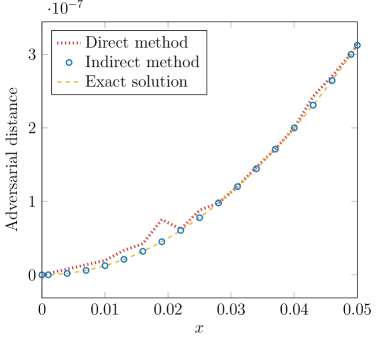
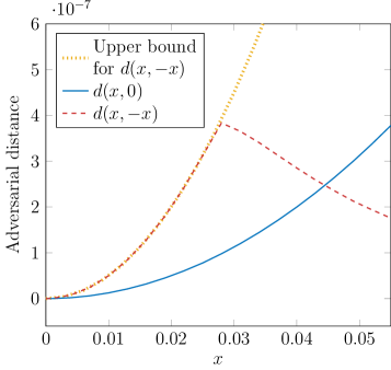
We use both direct and indirect methods to find $d(x,0)$ and compare the results with the exact solution given in (33). The parameters of the model are $L=2000$ km and $\gamma=1.27~{}\text{W}^{-1}\text{km}^{-1}$. The results are depicted in Fig. 1. Our conclusion is that the use of an indirect method usually results in a more accurate estimate of the distance. Hereinafter, we only use the indirect method of Theorem 4 for our numerical computations.

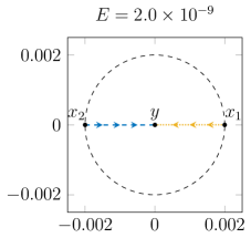
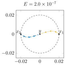
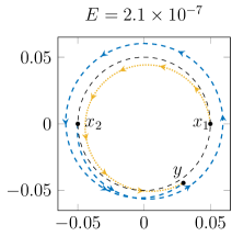
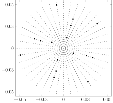
It is interesting to look at the optimum trajectories described by Theorem 4. We have solved the equations of Theorem 4 numerically for three pairs of $(x_{1},x_{2})$. In all three cases, we have chosen two antipodal input points, i.e., $x_{2}=-x_{1}=x$. Three different magnitudes for $x$ are considered, corresponding to different input powers. The trajectories of evolution of $x_{1}$ and $x_{2}$ that are obtained by the optimum adversarial noise are depicted in Fig. 2. It is evident that the strategy of the adversary varies as the input power is increased. In particular, for lower input powers, the optimum trajectory is obtained by confusing the two points at the origin. The adversary, in this case, needs to make enough effort to bring each point to the origin (see also (31)). At very high input powers, on the contrary, confusing the two points $x,-x$ through phase changes requires less effort (see Theorem 7, also see the argument on Fermat’s spiral in [49]).

(a) Small input power

(b) Medium input power

(c) Large input power

Figure 2: The trajectories of evolution of two input points corresponding to the optimum adversarial noise for three different input powers are depicted. The title of each figure represents the amount of adversarial effort needed to make the two points indistinguishable.

VI Constellation Design

One important application of the distance defined in Section III is to design signal constellations. Just as Euclidean distance can be used to position input signals for an AWGN channel, the adversarial distance of Section III can be used to provide guidelines when designing a signal constellation for the per-sample channel. Unlike the classical AWGN channel, where one can design a constellation for unit input peak/average power and then scale up/down the constellation points by a constant scalar based on the required power constraint, the design of a constellation for a nonlinear channel, such as the one we consider in this paper, is drastically different. In particular, the design of a constellation for a given average input power seems to be more difficult for the channel model of this paper as it requires the knowledge of the distance $d(\cdot,\cdot)$ for practically all points of $\mathbb{C}^{2}$. Finding a way to alleviate this problem is out of the scope of this introductory paper and is left for the future research (see also Section VII and VIII-A). Henceforth, we consider a peak power constraint for our constellation design problems.

In our first example, we calculate the distance between the two points of a binary antipodal constellation and an on-off keying constellation, and compare these two constellations for various peak powers. Then, we explain how we can design larger constellations with the largest minimum distance possible for a given peak power using clique-finding algorithms. A 16-point constellation with maximum minimum-distance for a fixed peak power is found to illustrate the ideas. The performance, in terms of symbol error rate (SER), of our proposed constellation is compared with that of the standard quadrature amplitude modulation (QAM) of the same size and peak power when the amplifier noise is assumed white (in space) and Gaussian.

VI-A Antipodal Versus On-Off Keying

We use numerical tools to find the distance $d(x,-x)$ for binary antipodal constellations with different input powers, as well as the closed-form equation for $d(x,0)$ corresponding to on-off keying constellations. The optical fiber parameters are the same as in Section V. The results are plotted in Fig. 3. For small input powers, $d(x,-x)$ matches the upper bound (29). In this “linear regime” the adversarial distance agrees with the Euclidean distance. One can see that the distance measure for an antipodal constellation shows a phase transition at around $x=0.03$. Eventually, at high input powers, it is seen that the points of the on-off keying constellation require a higher amount of adversarial effort to become indistinguishable. Hence, at high input powers, on-off keying is preferred over the antipodal scheme of the same peak power. From Fig. 3, it seems

$$\lim_{\lvert x\rvert\to\infty}d(x,-x)=0.$$ (34)

The following theorem generalizes this observation.

Theorem 7

Let $\phi\in[-\pi,\pi)$. Then

$$\lim_{\lvert x\rvert\to\infty}d(x,xe^{i\phi})=0.$$ (35)

Proof:

See Appendix F. ∎

Using similar techniques as in the proof of Theorem 7, one can show that if one of the two points has high power, the distance between the two points becomes the radial distance between them. This is summarized in the following corollary.

Corollary 2

For any $\theta_{1},\theta_{2}$ and $\Delta R$, we have

$$\lim_{R\to\infty}d(Re^{i\theta_{1}},(R+\Delta R)e^{i\theta_{2}})=\lim_{R\to\infty}d_{\text{R}}(Re^{i\theta_{1}},(R+\Delta R)e^{i\theta_{2}})=\frac{\Delta R^{2}}{4L}.$$ (36)

VI-B Constellation Design

The minimum distance of a constellation $\mathcal{C}$ is defined by

$$d(\mathcal{C})\triangleq\min\left\{\,d(x_{1},x_{2})\mid x_{1},x_{2}\in\mathcal{C},\,x_{1}\neq x_{2}\,\right\}.$$ (37)

Having the distances of all pairs of points on a grid, subject to a certain peak power, one can find a multi-point constellation with the largest minimum distance possible. The procedure we outline here is not specific to the adversarial distance of this paper and can be used to find a constellation with a prescribed size from a finite set of points equipped with a semimetric [50]. Let $G$ be a grid of points and assume that

$$d:G\times G\twoheadrightarrow D\subset\mathbb{R}$$ (38)

where $D$ is the range of $d(\cdot,\cdot)$ when restricted to $G\times G$. We form a sorted list of all elements of $D$. We then consider a threshold distance $d_{\text{th}}$ in $D$ and form a simple graph with vertex set $G$. Two vertices are connected by an edge if and only if their distance is at least $d_{\text{th}}$. In this graph, we then find a maximal clique [51]. If the size of the maximal clique is larger (smaller) than the prescribed constellation size, we choose a larger (smaller) $d_{\text{th}}$ from $D$. If the size of the maximal clique obtained this way is exactly equal to the prescribed value, and choosing a larger $d_{\text{th}}$ results in a strictly smaller maximal clique, then the obtained constellation has the largest minimum distance possible.

We start off by fixing a polar grid of points as candidates for our constellation points. We consider twenty different radii equally spaced between 0 and 0.05 together with forty different phases at each radius. The peak power of $0.5^{2}$ is selected so that the effect of nonlinearity becomes prominent (see Fig. 3). We use rotational symmetry to reduce the number of times the differential equations of Theorem 4 needs to be solved. Fig. 4 shows a 16-point constellation with maximum minimum-distance.

Figure 3: The distances $d(x,-x)$ for binary antipodal constellation (dashed) and $d(x,0)$ for on-off keying constellation (solid) are depicted. The upper bound of Theorem 6 is also shown (dotted).

VI-C Noise with Gaussian Statistics

In this subsection, we study the performance of the constellation given in Fig. 4 in terms of SER. To set up the simulations, we consider the channel model

$$\frac{d}{dz}q(z)=i\gamma\lvert q(z)\rvert^{2}q(z)+N(z),\quad 0\leq z\leq L\,.$$ (39)

where $N(z)$ is a complex white Gaussian process with vanishing pseudo-autocovariance and autocorrelation function

$$\mathsf{E}[N(z)N^{*}(z^{\prime})]=\sigma^{2}\delta(z-z^{\prime}).$$ (40)

The signal constellations that we can design based on the geometric approach of this paper are not necessarily optimum in terms of SER for the stochastic channel model of (39). Such constellation optimization has been considered before [26, 52]. In particular, in [52], for a target constellation size, a bank of amplitude phase-shift keying constellations are considered. The best constellation in terms of SER is then selected based on the results of simulations for each average input power. The size of the collection of constellations that is considered in [52] grows exponentially with the constellation size which renders their method impractical for larger constellations. Nevertheless, our objective in this section is not to compare the performance of the schemes designed in this paper with the exhaustive method of [52]. One should also note that we consider a peak power constraint as opposed to the average power constraint of [52]. We prefer to compare our design with the standard QAM constellation which seems to be a more natural baseline for us.

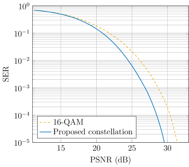
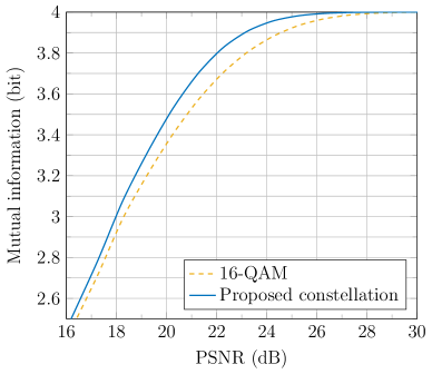
The SER of the optimal 16-point constellation of Fig. 4 and a conventional 16-QAM of the same peak power are illustrated in Fig. 5. To obtain SER of each constellation, the channel model of (39) is simulated by considering a fiber of length 2000 km as a concatenation of noise-free fibers of length 1 km each and injecting a Gaussian noise with variance $\sigma^{2}$ at the output of each fiber segment of length 1 km. Each constellation point is transmitted a total of 250,000 times. A fine 2 dimensional histogram is used to capture the empirical conditional distribution of the channel. All points of a constellation are chosen with the same probability. The mutual information for the two constellation under study is also estimated and is depicted in Fig. 6 for a range of $\sigma^{2}$. The horizontal axis in Fig. 6 is labeled by peak signal to noise ratio (PSNR).

Figure 4: Optimum 16-point constellation (dark points), subject to peak power of $0.05^{2}$ W, are selected from the depicted polar grid (light points).

Figure 5: The SER for the 16-point constellation proposed in this paper (solid) and a 16-QAM of the same peak power (dashed) is plotted. Fiber length is assumed $L=2000$ km and $\gamma=1.27$.

Figure 6: The mutual information with uniform input distribution for the 16-point constellation proposed in this paper (solid) and a 16-QAM of the same peak power (dashed) is plotted. Fiber length is assumed $L=2000$ km and $\gamma=1.27$.

VII Approximating the Adversarial Distance

When designing large constellations, the adversarial distance is useful only if the calculation of distance between two points is numerically feasible. However, finding the exact distance between two points requires solving a system of differential equations which is computationally expensive. For this reason, we propose an approximation for the adversarial distance that is numerically feasible and can be used when designing larger constellations. In this section, we first motivate the functional form that we use for our distance measure approximation and provide a recipe to find the parameters of our approximation. We then use the obtained approximation to design a (suboptimal) constellation of size 64 and compare its performances with a conventional QAM constellation of the same size and peak power constraint.

When we want to study the distance between two complex points, because of the rotational symmetry, we can safely assume that one of the points is real. Consider the distance $d(x,ye^{i\phi})$ with $x,y\in\mathbb{R}$ and $\phi\in[-\pi,\pi)$. For a fixed pair $(x,y)$, the distance $d(x,ye^{i\phi})$ is a function of the angle $\phi$. We already know that the radial distance is a natural attainable lower bound for the distance, i.e.,

$$d(x,ye^{i\phi})\geq d_{\text{R}}(x,y).$$ (41)

The angle that achieves the lower bound of (41) is denoted as

$$\phi^{*}(x,y).$$

That is, $d(x,ye^{i\phi^{*}(x,y)})=d_{\text{R}}(x,y)$. Using the same ideas that led to Theorem 5, we can prove the following lemma.

Lemma 1

For any $x,y\in\mathbb{R}$,

$$\phi^{*}(x,y)=\frac{L\gamma}{2}\left(x^{2}-y^{2}\right).$$

In the absence of nonlinearity, i.e., when $\gamma=0$, the adversarial distance reduces to a constant multiple of the squared Euclidean distance (see Section VIII). In this case, we denote the distance as

$$d_{\text{E}}(\cdot,\cdot)$$

where E in the subscript stands for Euclidean. Using the law of cosines, one can show that

$$d_{\text{E}}(x,ye^{i\phi})=d_{\text{R}}(x,y)+\frac{xy}{2L}\sin^{2}\left(\frac{\phi}{2}\right).$$ (42)

Motivated by (41) and (42), we assume the following functional form to approximate our adversarial distance when $\gamma\neq 0$:

$$d(x,ye^{i\phi})\approx d_{\text{R}}(x,y)+A(x,y)\sin^{2}\left(\frac{\phi-\phi^{*}(x,y)}{2}\right).$$ (43)

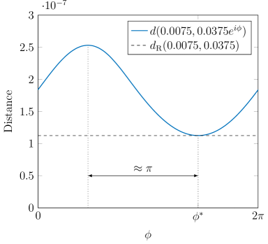
The bivariate function $A(x,y)$ in (43) represents the maximum deviation of the distance $d(x,ye^{i\phi})$ from the radial distance. The value of $d(x,ye^{i\phi})$ for a typical pair of $(x,y)$ is depicted in Fig. 7. From the numerical calculations of the distance, it seems that for a fixed $(x,y)$, the maximum deviation from the radial distance happens at the angle

$$\phi=\phi^{*}(x,y)-\pi$$

when properly interpreted as an angle in $[-\pi,\pi)$. We were not able to prove this observation mathematically. Nevertheless, as we are looking for an approximation, confirmation with numerical data serves our purpose. The problem of distance approximation, therefore, reduces to finding a good approximation for the bivariate function $A(x,y)$. To this end, we numerically calculate the distance

$$d(x,ye^{i\left(\phi^{*}(x,y)-\pi\right)})$$

for various pairs of $(x,y)$ with high resolution. We then use a bilinear interpolating fit to obtain a symmetric expression for $A(x,y)$. Lastly, we generalize the approximation formula (43) to complex pairs using the rotational symmetry. If

$$(x,y)\in\mathbb{R}^{2},\quad(\phi_{x},\phi_{y})\in[-\pi,\pi)^{2},$$

we have

$$d(xe^{i\phi_{x}},ye^{i\phi_{y}})\approx d_{\text{R}}(x,y)+A(x,y)\sin^{2}\left(\frac{\phi_{y}-\phi_{x}-\phi^{*}(x,y)}{2}\right).$$ (44)

Note that the symmetry property of the distance is captured by this approximation form only if $A(x,y)$ is symmetric itself. We make sure that the symmetry on $A(x,y)$ is enforced by taking the average of $A(x,y)$ and $A(y,x)$ in our numerical calculations. Interestingly, even without this symmetrization, the numerical calculations of $A(x,y)$ show that this function is (up to numerically significant figures) symmetric.

Figure 7: The distance $d(x,ye^{i\phi})$ for a fixed $(x,y)$ is plotted as a function of $\phi$. The maximum deviation from the radial distance is (approximately) achieved at $\phi^{*}(x,y)-\pi$.

Figure 8: A suboptimal 64-point constellation (dark points), subject to peak power of $0.05^{2}$ W.

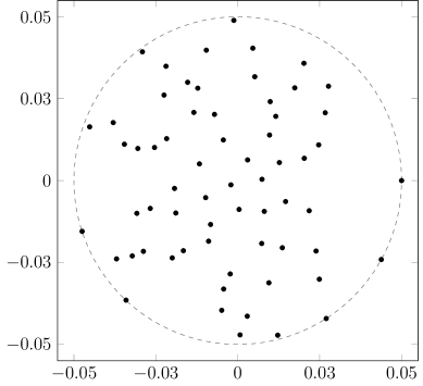
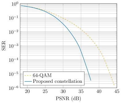
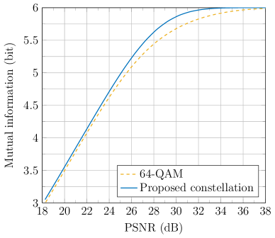
Using the approximate form (44), one can think of algorithms that find large constellations with large minimum distances. The methodology of Section VI may not be computationally feasible for larger constellations. Hence, one can use various greedy suboptimal methods for designing constellations with large minimum distances. For instance, for a randomly selected initial constellation, we “slightly move the constellations points, one at a time, in either radial or azimuthal direction with a fixed step size until no improvement in the minimum distance of the constellation is observed. The step size is then halved and the procedure is repeated until no significant change is observed. We use this method to find a suboptimal constellation of size 64 with 10,000 trials. At each trial, the points of the initial random constellation are selected randomly subject to the peak power constraint $0.05^{2}$. The best constellation—one with the largest minimum distance—that we obtained is shown in Fig. 8. The SER and mutual information with uniform input distribution of this constellation are shown in Fig. 9 and Fig. 10.

Figure 9: The SER for the 64-point constellation proposed in this paper (solid) and a 64-QAM of the same peak power (dashed) is plotted. Fiber length is assumed $L=2000$ km and $\gamma=1.27$.

Figure 10: The mutual information with uniform input distribution for the 64-point constellation proposed in this paper (solid) and a 64-QAM of the same peak power (dashed) is plotted. Fiber length is assumed $L=2000$ km and $\gamma=1.27$.

VIII Discussion

In this section, we outline potential extensions of the variational approach considered in this paper. We first explain how to find the distance with respect to a normalized problem. We then discuss the problem of minimum distance decoding based on the distance measure introduced in this paper. Then, we explain how we can readily extend the analysis of this paper to the nondispersive waveform channel. It is also shown how one can use the approach of this paper for a class of linear channels. We also briefly review the possibility of extending our model to the general case of (1). Other discussions include the possibility of extending the set $F$ of possible adversarial noise trajectories. The problem of designing input signal spaces based on the proposed adversarial distance is also briefly discussed. Finally, we comment on the analogy of the adversarial concepts of this paper and their relation to concepts in non-stochastic information theory.

VIII-A Dimensionless Equation

Recall that the channel law of this paper is described by the per-sample channel model, which we repeat here for convenience

$$\frac{d}{dz}q(z)=i\gamma\lvert q(z)\rvert^{2}q(z)+n(z),\quad 0\leq z\leq L.$$ (45)

If we consider the following change of variables

$$\mathtt{z}=\frac{z}{L},\quad\mathtt{q}(\mathtt{z})=\sqrt{\gamma L}q(\mathtt{z}L),$$ (46)

what we get is

$$\frac{d}{d\mathtt{z}}\mathtt{q}(\mathtt{z})=i\lvert\mathtt{q}(\mathtt{z})\rvert^{2}\mathtt{q}(\mathtt{z})+\mathtt{n}(\mathtt{z}),\quad 0\leq\mathtt{z}\leq 1$$ (47)

with

$$\mathtt{n}(\mathtt{z})=L\sqrt{\gamma L}n(\mathtt{z}L).$$ (48)

One can use this normalized equation to define the distance between two points $\mathtt{x_{1}},\mathtt{x_{2}}$, denoted as

$$\mathtt{d}(\mathtt{x_{1}},\mathtt{x_{2}}).$$ (49)

Using the normalized distance (49), one can find the distance in physical units by

$$d(x_{1},x_{2})=\frac{\mathtt{d}(\mathtt{x_{1}},\mathtt{x_{2}})}{L^{2}\gamma}$$ (50)

with

$$\mathtt{x_{1}}=\sqrt{\gamma L}x_{1},\quad\mathtt{x_{2}}=\sqrt{\gamma L}x_{2}.$$

This allows for solving the distance problem for the dimensionless equation (47) independent of the fiber parameters $\gamma$ and $L$, and then use (50) based on the actual fiber parameters of a particular system.

VIII-B Minimum Distance Decoder

Having a notion of distance, we can consider a minimum distance decoder which produces the constellation point that requires the least amount of adversarial effort to reach to the received point at the output of the channel. Let $y$ denote the point received at the output of the channel. Define

$$E(x,y)=\inf\{\varepsilon\mid y\in B_{\varepsilon}(x)\}.$$ (51)

That is, $E(x,y)$ is the minimum adversarial effort needed to transform $x$ to $y$ through the nonlinear channel of (2). The minimum distance decoder, for a constellation $\mathcal{C}$, then decides on

$$\hat{x}=\mathsf{DEC}_{\text{MD}}(y)\triangleq\arg\min_{x\in\mathcal{C}}E(x,y)\,,$$ (52)

where ties are broken arbitrarily. Minimum distance decoding, therefore, requires calculation of $E(x,y)$ for all points $x$ in $\mathcal{C}$. Using techniques similar to the proof of Theorem 4, one can prove the following Theorem.

Theorem 8

If the trajectory

$$q(z)=a(z)+ib(z)$$ (53)

minimizes the adversarial effort needed to transform $x$ to $y$, then

$$-4\gamma b^{\prime}(a^{2}+b^{2})+3\gamma^{2}a(a^{2}+b^{2})^{2}-a^{\prime\prime}=0$$ ,

$$4\gamma a^{\prime}(a^{2}+b^{2})+3\gamma^{2}b(a^{2}+b^{2})^{2}-b^{\prime\prime}=0$$ ,

together with the boundary conditions at $z=0$ given by

$$a(0)+ib(0) = x,$$

and at $z=L$ given by

$$a(L)+ib(L)=y.$$

Theorem 8 implies that a system of ODEs needs to be solved to find out the minimum adversarial effort that has caused the received symbol from any of the constellation points. If written in polar coordinates, the system of ODEs in Theorem 8 turns into a system of first oder nonlinear ODEs (see (A7) in [8]) that can be solved analytically. The problem, then, reduces to a system of nonlinear algebraic equations in terms of the boundary conditions. Solving such nonlinear algebraic equation may still be numerically expensive. In that case, once the constellation is fixed, these calculations need to be done only once. One can, then, quantize the complex plane using a fine grid and compute the distance of each point of the grid from the constellation points. Each grid point is then labeled with the constellation point closest to it in terms of the adversarial distance. These labels can be stored in a look-up table and can be read at the time of decoding.

VIII-C From the Per-Sample Channel to the Waveform Channel

Consider the channel model that is described by the evolution equation

$$\frac{\partial}{\partial z}q(z,t) = i\gamma\lvert q(z,t)\rvert^{2}q(z,t)+n(z,t),$$

$$0\leq z\leq L -T\leq t\leq T.$$ , (54)

The input alphabet $\mathcal{X}$ and the output alphabet $\mathcal{Y}$ for this channel are the set of component-wise continuously differentiable complex functions defined on $[-T,T]$. The channel input $x(t)$ is described by the boundary condition $q(0,t)=x(t)$. Similarly, the channel output $y(t)$ is the signal at $z=L$, i.e., $y(t)=q(L,t)$. Similar to Section II, we describe the nonlinear relation between the input $x$, the output $y$, and the adversarial noise $n(z,t)$ by writing

$$y=N(x,n).$$

If $y=N(x,n)$ and

$$E=\int_{0}^{L}\int_{-T}^{T}{\lvert n(z,t)\rvert^{2}}\,dt\,dz\,,$$

we write

$$x\overset{E}{\to}y\,.$$

Define

$$S_{E}(x)=\left\{\,y\mid x\overset{E}{\to}y\,\right\}.$$

The noise balls are defined in the same way as in Section II by

$$B_{E}(x)=\bigcup_{\epsilon\leq E}{S_{\epsilon}(x)}.$$

Finally, for any $x_{1}$ and $x_{2}$ in $\mathcal{X}$, define

$$D(x_{1},x_{2})\triangleq\inf\left\{\,E\mid B_{E}(x_{1})\cap B_{E}(x_{2})\neq\varnothing\,\right\}.$$ (55)

Because the channel acts on different time-samples of the signal independently, the waveform distance $D(\cdot,\cdot)$ is related to the per-sample distance $d(\cdot,\cdot)$ by

$$D(x_{1},x_{2})=\int_{-T}^{T}{d(x_{1}(t),x_{2}(t))}\,\mathit{dt}.$$ (56)

Although moving from the per-sample channel to the waveform channel is completely described by (56), the problem of designing constellations with maximum minimum-distance in this case is slightly more complicated. We do not intend to address this problem here, but one may consider further restriction on the input set so that the problem becomes feasible. For instance, the input set may be limited to a set of waveforms of particular shapes (e.g., truncated square root raised cosines or rectangular pulses).

VIII-D Application to Linear Channels

Consider the class of channels defined by the linear evolution equation

$$\frac{\partial}{\partial z}q(z,t) = \sum_{j=0}^{J}{a_{j}\frac{\partial^{j}}{\partial t^{j}}q(z,t)}+n(z,t),$$

$$0\leq z\leq L -T\leq t\leq T,$$ , (57)

where $a_{j}$ are complex constants. The input alphabet $\mathcal{X}$ and the output alphabet $\mathcal{Y}$ are the set of $J$ times component-wise continuously differentiable complex functions defined on $[-T,T]$. We further assume that the functions in $\mathcal{X}$ and $\mathcal{Y}$ satisfy Dirichlet conditions (so that they have a Fourier series representation) and that the functions themselves and all of their derivatives vanish at the boundaries $t=\pm T$ (so that the derivative of their Fourier series is the Fourier series of their derivative). We wish to find a set of necessary conditions similar to Theorem 4 that characterizes the adversarial noise trajectories of least energy that confuse two input waveforms $x_{1}(t)$ and $x_{2}(t)$. The linearity of the evolution equation (VIII-D) greatly simplifies the analysis as opposed to the nonlinear evolution of the per-sample channel. Let the Fourier series representation of $x_{k}(t)$ be

$$x_{k}(t)=\sum_{m}X_{m}^{(k)}e^{i\omega_{m}t},\quad k=1,2,$$ (58)

where

$$\omega_{m}=\frac{m\pi}{T}.$$ (59)

Also, let the state variable that describes the evolution of $x_{1}$ be $q(z,t)$ and the state variable that describes the evolution of $x_{2}$ be $p(z,t)$. Let the Fourier series coefficients of $q(z,t)$ and $p(z,t)$ be $Q_{m}(z)$ and $P_{m}(z)$, respectively. The channel law in (VIII-D) can be identified by a channel polynomial

$$R(x)=\sum_{j=0}^{J}{a_{j}x^{j}}.$$ (60)

With these notations, we summarize the results in Theorem 9.

Theorem 9

The trajectories $q(z,t)$ and $p(z,t)$ that minimize the effort needed to confuse $x_{1}$ and $x_{2}$ satisfy the following system of equations:

$$Q_{m}(z)=\left\{\begin{array}[]{ll}\!\left(A_{m}\!+\!B_{m}z\right)e^{R(i\omega_{m})z}&\mbox{if }\operatorname{Re}{R(i\omega_{m})}=0,\\ \!A_{m}e^{R(i\omega_{m})z}\!+\!B_{m}e^{-R^{*}(i\omega_{m})z}&\mbox{otherwise},\end{array}\right.$$

$$P_{m}(z)=\left\{\begin{array}[]{ll}\!\left(C_{m}\!+\!D_{m}z\right)e^{R(i\omega_{m})z}&\mbox{if }\operatorname{Re}{R(i\omega_{m})}=0,\\ \!C_{m}e^{R(i\omega_{m})z}\!+\!D_{m}e^{-R^{*}(i\omega_{m})z}&\mbox{otherwise},\end{array}\right.$$

with the boundary conditions at $z=0$

$$Q_{m}(0) = X^{(1)}_{m},$$ (61)

$$P_{m}(0) = X^{(2)}_{m},$$ (62)

and at $z=L$

$$Q_{m}(L)=P_{m}(L),$$ (63)

together with

$$(1-\mu)B_{m}+\mu D_{m}=0,$$ (64)

$$\sum_{m}{f(R(i\omega_{m}))\left(\lvert B_{m}\rvert^{2}-\lvert D_{m}\rvert^{2}\right)}=0,$$ (65)

with

$$f(x)=\left\{\begin{array}[]{ll}1&\mbox{if }\operatorname{Re}{x}=0,\\ \left(x+x^{*}\right)\left(e^{-L\left(x+x^{*}\right)}-1\right)&\mbox{otherwise}.\end{array}\right.$$ (66)

Proof:

The proof is very similar to the proof of Theorem 4. ∎

Note that Theorem 9 describes the optimal trajectories as a system of algebraic equations. If we assume that both $q$ and $p$ are (approximately) bandlimited and we only have $2M+1$ nonzero frequency taps in their Fourier series representations, i.e.,

$$q(z,t) = \sum_{m=-M}^{M}{Q_{m}(z)e^{i\omega_{m}t}},$$ (67)

$$p(z,t) = \sum_{m=-M}^{M}{P_{m}(z)e^{i\omega_{m}t}},$$ (68)

then, Theorem 9 gives $4\times(2M+1)+1$ equations in the unknowns

$$A_{m},B_{m},C_{m},D_{m},$$

and the Lagrange multiplier $\mu$. This is much easier to solve than the system of differential equations that appears in the nonlinear case.

Example 1

In this example, we consider the channel described by the nonlinear Schrödinger equation (1) when $\gamma=0$. For this dispersive channel, the channel polynomial is

$$R(x)=-i\frac{\beta_{2}}{2}x^{2}.$$ (69)

One can easily show that $\mu=1/2$ and

$$Q_{m}(z) = \left(X^{(1)}_{m}+\frac{X^{(2)}_{m}-X^{(1)}_{m}}{2L}z\right)e^{i\frac{\beta_{2}}{2}\omega_{m}^{2}z},$$ (70)

$$P_{m}(z) = \left(X^{(2)}_{m}-\frac{X^{(2)}_{m}-X^{(1)}_{m}}{2L}z\right)e^{i\frac{\beta_{2}}{2}\omega_{m}^{2}z},$$ (71)

and that

$$d(x_{1},x_{2}) = \sum_{m}\frac{\lvert X^{(2)}_{m}-X^{(1)}_{m}\rvert^{2}}{4L}$$ (72)

$$= \frac{1}{8LT}\int_{-T}^{T}\left\lvert{x_{2}(t)-x_{1}(t)}\right\rvert^{2}\,dt\,,$$ (73)

which is proportional to the squared Euclidean distance between $x_{1}$ and $x_{2}$.

VIII-E Extension to the Nonlinear Schrödinger Equation

It is possible to extend the adversarial model of this paper to the general case of the optical fiber described by (1). Instead of a complex number, the input of the channel is a complex function described by the boundary condition at $z=0$, i.e.,

$$x(t)=q(0,t),\quad t\in[-T,T].$$

The input alphabet may be restricted to the functions that decay sufficiently rapidly within the time frame $[-T,T]$. The number $T$ should be chosen large enough to capture the dispersive effect of the fiber. One can also think of letting $T\to\infty$. The output of the channel, then, is

$$y(t)=q(L,t),\quad t\in[-T,T].$$

The adversarial effort can be generalized to

$$e=\int_{0}^{L}\int_{-T}^{T}\lvert n(z,t)\rvert^{2}\,dt\,dz.$$

One can then formulate the distance between two input signals as a more general variational problem. Unlike the per-sample channel of this paper that has only one degree of freedom, the extension to the nonlinear Schrödinger equation has many degrees of freedom. To find out if the distance measure formulated here can be found in a tractable way is a subject for future research.

We should also mention that it is possible to consider other types of adversarial effort. We chose energy as at seems to be the most natural quantity. One may also relate the common probabilistic model to the adversarial model by considering the maximum effort of the “typical” noise trajectories in the probabilistic model and consider the adversaries with limited effort accordingly.

VIII-F Generalizing Adversarial Noise Trajectories

In defining the distance $d(\cdot,\cdot)$, we assumed that the adversarial noise trajectories are continuous functions of $z$. It is possible to extend the class of possible adversarial noise trajectories $F$ so that they have a finite number of discontinuities. That is, $F$ is the set of piecewise continuous functions from $[0,L]$ to $\mathbb{C}$. We will not pursue this assumption here. We only mention that it is possible to solve the variational problem (13) by considering extra Weierstrass–Erdmann conditions at the points of discontinuity [40].

VIII-G Code Design

The average power of a constellation $\mathcal{C}$ is defined by

$$P(\mathcal{C})\triangleq\frac{1}{\lvert\mathcal{C}\rvert}\sum_{x\in\mathcal{C}}\lvert x\rvert^{2}.$$ (74)

The following design question can be asked:

• Given two positive numbers $d_{\text{min}}$ and $P_{\text{ave}}$, design a constellation $\mathcal{C}$ having $d(\mathcal{C})\geq d_{\text{min}}$ and $P(\mathcal{C})\leq P_{\text{ave}}$, with $\lvert\mathcal{C}\rvert$ as large as possible.

This question can be thought of as a packing problem. Naturally, a Gilbert–Varshamov-type argument [55] may be used to find a lower bound on the size of a constellation.

VIII-H Relation to Non-stochastic Information Theory

The adversarial noise model of this paper is closely related to the non-stochastic framework of [35, 56, 57]. The input and output of the channel model of this paper can be thought of as two uncertain variables (UVs) [35]. The peak power constraint together with the adversarial distance considered in this paper define a bounded semimetric space for the range $\llbracket X\rrbracket$ of the input UV $X$. The noise ball $B_{E}(x)$ is equivalent to the conditional range $\llbracket Y\mid x\rrbracket$, where $Y$ is the output UV. Similarly, finding the largest signal constellation with $d_{\text{min}}>E$ is equivalent to the $(E,0)$-capacity of [56, 57] or the Kolmogorov $2E$-capacity [58]. This analogy shows the intimate connection between reachability analysis of bounded perturbation in control theory and non-stochastic information theory. It would be interesting to see whether or not one can use the framework of non-stochastic information theory to estimate the capacity of nonlinear channels such as the one considered in this paper (see also [49]).

IX Conclusions

We have proposed an adversarial model for the nondispersive optical fiber channel, and given necessary conditions for the energy-minimizing adversarial noise. By means of numerical methods, we have shown that the optimum noise trajectories show different trends in different input-power regimes. The adversarial distance of this paper is used to design large constellations that outperform conventional QAM constellations in terms of SER.

This paper outlines only the very first steps toward a new way of studying the nonlinear interaction of the signal and noise in optical fiber. It remains to see whether this model can be used to design new fiber-optic communication schemes.

Appendix A Proof of Theorem 1

To prove the uniqueness of the solution of the state equation (4), we use the following theorem (see [59, p. 94]):

Theorem 10

Let $g(q,z)$ be continuous in $z$ and locally Lipschitz in $q$ for all $z\in[0,L]$ and all $q$ in a domain $D\subset\mathbb{C}$. Let $W$ be a compact subset of $D$, $x\in W$, and suppose that it is known that every solution of

$$q^{\prime}=g(q,z),\quad q(0)=x$$ (75)

lies entirely in $W$. Then, there is a unique solution that is defined for all $z\in[0,L]$.

For us, the function $g(\cdot,\cdot)$ is given by

$$g(q,z)=f(q)+n(z).$$ (76)

The continuity of $n(z)$ guarantees the continuity of $g(q,z)$ in $z$. It is also straightforward to show that the function

$$f(q)=i\gamma\lvert q\rvert^{2}q$$ (77)

is locally Lipschitz for all $q\in\mathbb{C}$. We only need to show that, for any given control signal $n(z)$, any solution of (75) lies in a compact subset of $\mathbb{C}$. Equivalently, we show that any solution has a bounded magnitude.

To prove the boundedness of $q$, we rewrite the state equation in polar coordinates. Let

$$q(z)=R(z)e^{i\theta(z)}.$$ (78)

If

$$N_{0}=\max_{z}\lvert n(z)\rvert,$$ (79)

then by using the Cauchy–Schwarz inequality and (20), one can show that

$$R^{\prime}\leq N_{0}.$$ (80)

From this, we have

$$R(z)\leq R(0)+zN_{0}\leq R(0)+LN_{0}.$$ (81)

Appendix B Proof of Theorem 2

After the uniqueness of the solution is established (see Theorem 1), one can multiply both sides of (4) by the integrating factor

$$e^{-i\gamma\int_{0}^{z}\lvert q(s)\rvert^{2}\,ds}$$ (82)

and integrate over $z$.

Appendix C Proof of Theorem 3

The linearized control system corresponding to the state equation (4) along the trajectory of $q(0)=x$ and $n(z)$ is defined by

$$Q^{\prime}=f^{\prime}(q(z))Q(z)+U(z)$$ (83)

where $Q(z)$ is the state of the linearized system, $U$ is the control and $q(z)$ is the unique solution of (4) with the initial condition $q(0)=x$ and the control signal $n(z)$. Also, $f^{\prime}(q)$ is the Jacobi matrix with the two variables of $f(\cdot)$ being the real and the imaginary parts of $q$.

The nonlinear system is locally controllable along $q$, if the linear time-variant system (83) is controllable (see [39, Theorem 3.6]). The control signal in the linearized system is acting additively. Hence, from [39, Theorem 1.18], the linearized system is controllable.

Appendix D Proof of Theorem 4

This theorem is an example of problems in optimal control theory with some extra boundary conditions [60]. We sketch a proof for the sake of completeness. To follow all of the steps, some familiarity with calculus of variations may be needed (see [40]).

First, we rewrite the energy constraint

$$\int_{0}^{L}{\sum_{k=1}^{2}(-1)^{k}g_{k}(a_{k},b_{k},a_{k}^{\prime},b_{k}^{\prime})}dz=0$$ (84)

as a differential equation and then incorporate this condition into the optimization using a Lagrange multiplier. Define

$$c(z)=\int_{0}^{z}\sum_{k=1}^{2}(-1)^{k}g_{k}(a_{k},b_{k},a_{k}^{\prime},b_{k}^{\prime})\,dz.$$ (85)

Then

$$c^{\prime}(z)=\sum_{k=1}^{2}(-1)^{k}g_{k}(a_{k},b_{k},a_{k}^{\prime},b_{k}^{\prime}),$$ (86)

with the boundary conditions

$$c(0)=c(L)=0.$$ (87)

Now we form the augmented Lagrangian

$$\mathcal{L}= g_{1}(a_{1},b_{1},a_{1}^{\prime},b_{1}^{\prime})$$

$$-\mu(z)\left(c^{\prime}-\sum_{k=1}^{2}(-1)^{k}g_{k}(a_{k},b_{k},a_{k}^{\prime},b_{k}^{\prime})\right),$$

where $\mu(z)$ is the Lagrange multiplier. Consider the action $s$ defined by

$$s=\int_{0}^{L}{\mathcal{L}(a_{1},a_{2},b_{1},b_{2},a_{1}^{\prime},a_{2}^{\prime},b_{1}^{\prime},b_{2}^{\prime},\mu,c^{\prime})}\,dz,$$ (89)

subject to the boundary conditions

$$a_{k}(0)+ib_{k}(0)=x_{k},$$ (90)

$$a_{1}(L)=a_{2}(L),$$ (91)

$$b_{1}(L)=b_{2}(L),$$ (92)

$$c(0)=c(L)=0.$$ (93)

We consider the variations of $s$, denoted as $\delta s$, caused by varying $a_{k}(z)$, $b_{k}(z)$, $\mu(z)$ and $c(z)$ while all boundary conditions are kept satisfied. Due to the energy constraint (86), the variations of $a_{k}(z)$, $b_{k}(z)$ and $c(z)$ are not independent and finding the explicit relation between them, for all $z$, is not easy. The Lagrange multiplier $\mu$ allows us to avoid this issue—similarly to the case of optimization problems in multi-variable calculus with nontrivial constraints.

We expand $\delta s$ in terms of $\delta a_{k}$, $\delta b_{k}$, $\delta\mu$ and $\delta c$ to get

$$\delta s=\int_{0}^{L}\bigg{[}\mathcal{L} \left(a_{1}+\delta a_{1},a_{2}+\delta a_{2},b_{1}+\delta b_{1},b_{2}+\delta b_{2},\right.$$

$$\left.\quad a_{1}^{\prime}+\delta a^{\prime}_{1},a_{2}^{\prime}+\delta a^{\prime}_{2},b_{1}^{\prime}+\delta b^{\prime}_{1},b_{2}^{\prime}+\delta b^{\prime}_{2},\right.$$

$$\quad\left.\mu+\delta\mu,c^{\prime}+\delta c^{\prime}\right)$$

$$-\mathcal{L}\left(a_{1},a_{2},b_{1},b_{2},a_{1}^{\prime},a_{2}^{\prime},b_{1}^{\prime},b_{2}^{\prime},\mu,c^{\prime}\right)\bigg{]}\,dz.$$

A Taylor series expansion to first order gives

$$\delta s= \int_{0}^{L}(1-\mu)\left(\frac{\partial g_{1}}{\partial a_{1}}\delta a_{1}+\frac{\partial g_{1}}{\partial a_{1}^{\prime}}\delta a_{1}^{\prime}\right)\,dz$$

$$+\int_{0}^{L}(1-\mu)\left(\frac{\partial g_{1}}{\partial b_{1}}\delta b_{1}+\frac{\partial g_{1}}{\partial b_{1}^{\prime}}\delta b_{1}^{\prime}\right)\,dz$$

$$+\int_{0}^{L}\mu\left(\frac{\partial g_{2}}{\partial a_{2}}\delta a_{2}+\frac{\partial g_{2}}{\partial a_{2}^{\prime}}\delta a_{2}^{\prime}\right)\,dz$$

$$+\int_{0}^{L}\mu\left(\frac{\partial g_{2}}{\partial b_{2}}\delta b_{2}+\frac{\partial g_{2}}{\partial b_{2}^{\prime}}\delta b_{2}^{\prime}\right)\,dz$$

$$-\int_{0}^{L}\mu\delta c^{\prime}\,dz$$

$$-\int_{0}^{L}\left(c^{\prime}-\sum_{k=1}^{2}(-1)^{k}g_{k}(a_{k},b_{k},a_{k}^{\prime},b_{k}^{\prime})\right)\delta\mu\,dz.$$

Note that because of the energy constraint (86), the coefficient of $\delta\mu$ is zero. Remember that a variation is feasible only if it respects the boundary conditions. For instance, because of the fixed boundary conditions at $z=0$, all variations must satisfy

$$\delta a_{k}(0)=\delta b_{k}(0)=0$$ (96)

Using (96), we integrate the terms having $\delta a_{k}^{\prime}$, $\delta b_{k}^{\prime}$ and $\delta c^{\prime}$ by parts and use the boundary conditions (90) and (93) to get

$$\delta s= \int_{0}^{L}\left((1-\mu)\frac{\partial g_{1}}{\partial a_{1}}-\frac{d}{dz}\left((1-\mu)\frac{\partial g_{1}}{\partial a_{1}^{\prime}}\right)\right)\delta a_{1}\,dz$$

$$+\int_{0}^{L}\left((1-\mu)\frac{\partial g_{1}}{\partial b_{1}}-\frac{d}{dz}\left((1-\mu)\frac{\partial g_{1}}{\partial b_{1}^{\prime}}\right)\right)\delta b_{1}\,dz$$

$$+\int_{0}^{L}\left(\mu\frac{\partial g_{2}}{\partial a_{2}}-\frac{d}{dz}\left(\mu\frac{\partial g_{2}}{\partial a_{2}^{\prime}}\right)\right)\delta a_{2}\,dz$$

$$+\int_{0}^{L}\left(\mu\frac{\partial g_{2}}{\partial b_{2}}-\frac{d}{dz}\left(\mu\frac{\partial g_{2}}{\partial b_{2}^{\prime}}\right)\right)\delta b_{2}\,dz$$

$$+\int_{0}^{L}\mu^{\prime}\delta c\,dz$$

$$+(1-\mu)\frac{\partial g_{1}}{\partial a_{1}^{\prime}}\delta a_{1}\Bigg{|}_{z=L}+(1-\mu)\frac{\partial g_{1}}{\partial b_{1}^{\prime}}\delta b_{1}\Bigg{|}_{z=L}$$

$$+\mu\frac{\partial g_{2}}{\partial a_{2}^{\prime}}\delta a_{2}\Bigg{|}_{z=L}+\mu\frac{\partial g_{2}}{\partial b_{2}^{\prime}}\delta b_{2}\Bigg{|}_{z=L}.$$

If $a_{k}^{*}(z)$, $b_{k}^{*}(z)$, $\mu^{*}(z)$ and $c^{*}(z)$ are minimizers of the action $s$, then

$$\delta s\Bigg{|}_{\begin{subarray}{c}a_{k}=a_{k}^{*},~{}b_{k}=b_{k}^{*},\\ \mu=\mu^{*},~{}c=c^{*}\end{subarray}}=0.$$ (98)

To have admissible variations, we must ensure that (90)–(93) are satisfied by all of the variations considered. We consider all $\delta c$ for which $\mu^{\prime}$ is orthogonal to $\delta c$. This allows us to pick arbitrary variations for $a_{k}$ and $b_{k}$ without violating the energy constraint (86). The boundary conditions (91)–(92) at $z=L$ imply

$$\delta a_{1}(L)=\delta a_{2}(L),$$

and

$$\delta b_{1}(L)=\delta b_{2}(L).$$

The trick is now to pick variations in such a way that all but one of the terms in (D) vanish. For instance, consider all admissible variations for which

$$\delta a_{1}(L)=0$$

and

$$\delta a_{2}(z)=\delta b_{1}(z)=\delta b_{2}(z)=0\,,z\in[0,L].$$

We then have

$$\int_{0}^{L}\left((1-\mu)\frac{\partial g_{1}}{\partial a_{1}}-\frac{d}{dz}\left((1-\mu)\frac{\partial g_{1}}{\partial a_{1}^{\prime}}\right)\right)\delta a_{1}\,dz=0.$$ (99)

From [40, Lemma 1 of Sec 1.3], we conclude that the integrand is zero, i.e.,

$$(1-\mu)\frac{\partial g_{1}}{\partial a_{1}}-\frac{d}{dz}\left((1-\mu)\frac{\partial g_{1}}{\partial a_{1}^{\prime}}\right)=0.$$ (100)

With appropriate selection of variations, one can show that the other terms with integrals in (D) are zero. Thus, (D) is simplified and we get

$$+(1-\mu)\frac{\partial g_{1}}{\partial a_{1}^{\prime}}\delta a_{1}\Bigg{|}_{z=L}+\mu\frac{\partial g_{2}}{\partial a_{2}^{\prime}}\delta a_{1}\Bigg{|}_{z=L}$$ (101)

$$+(1-\mu)\frac{\partial g_{1}}{\partial b_{1}^{\prime}}\delta b_{1}\Bigg{|}_{z=L}+\mu\frac{\partial g_{2}}{\partial b_{2}^{\prime}}\delta b_{1}\Bigg{|}_{z=L}=0.$$

If we consider those variations for which

$$\delta a_{1}(L)=0,$$

from (101) we get

$$\left((1-\mu)\frac{\partial g_{1}}{\partial b_{1}^{\prime}}+\mu\frac{\partial g_{2}}{\partial b_{2}^{\prime}}\right)\Bigg{|}_{z=L}=0.$$ (102)

Similarly, one can get

$$\left((1-\mu)\frac{\partial g_{1}}{\partial a_{1}^{\prime}}+\mu\frac{\partial g_{2}}{\partial a_{2}^{\prime}}\right)\Bigg{|}_{z=L}=0.$$ (103)

If we consider variations $\delta c$ for which $\mu^{\prime}$ is not necessarily orthogonal to $\delta c$, we can now consider arbitrary variations $\delta c$ and, with similar argument as in the previous paragraph, we must have

$$\int_{0}^{L}\mu^{\prime}\delta c\,dz=0.$$ (104)

Again, from [40, Lemma 1 of Sec 1.3], we conclude that

$$\mu^{\prime}=0,$$ (105)

i.e., the optimal Lagrange multiplier is a constant (as expected). Let $\mu^{*}(z)=\lambda$. The Euler-Lagrange conditions can now be simplified. These equations, together with the required energy constraint, become

$$(1-\lambda)\left(\frac{\partial g_{1}}{\partial a_{1}}-\frac{d}{dz}\left(\frac{\partial g_{1}}{\partial a_{1}^{\prime}}\right)\right)=0,$$

$$(1-\lambda)\left(\frac{\partial g_{1}}{\partial b_{1}}-\frac{d}{dz}\left(\frac{\partial g_{1}}{\partial b_{1}^{\prime}}\right)\right)=0,$$

$$\lambda\left(\frac{\partial g_{2}}{\partial a_{2}}-\frac{d}{dz}\left(\frac{\partial g_{2}}{\partial a_{2}^{\prime}}\right)\right)=0,$$

$$\lambda\left(\frac{\partial g_{2}}{\partial b_{2}}-\frac{d}{dz}\left(\frac{\partial g_{2}}{\partial b_{2}^{\prime}}\right)\right)=0,$$

$$c^{\prime}(z)=\sum_{k=1}^{2}(-1)^{k}g_{k}(a_{k},b_{k},a_{k}^{\prime},b_{k}^{\prime}).$$ (106)

The required boundary conditions are

$$a_{k}(0)+ib_{k}(0)=x_{k},$$

$$a_{1}(L)=a_{2}(L),$$

$$b_{1}(L)=b_{2}(L),$$

$$c(0)=c(L)=0,$$

$$\left((1-\lambda)\frac{\partial g_{1}}{\partial a_{1}^{\prime}}+\lambda\frac{\partial g_{2}}{\partial a_{2}^{\prime}}\right)\Bigg{|}_{z=L}=0,$$

$$\left((1-\lambda)\frac{\partial g_{1}}{\partial b_{1}^{\prime}}+\lambda\frac{\partial g_{2}}{\partial b_{2}^{\prime}}\right)\Bigg{|}_{z=L}=0.$$ (107)

There are four differential equations of second order and one of first order in (D). There are also ten boundary conditions in (D) together with one unknown $\lambda$. Hence, at least in principle, it is possible to solve these equations.

From these, after some algebraic manipulation, one obtains the equations given in Theorem 4.

Appendix E Proof of Theorem 6

Consider the state equation in polar coordinates $q(z)=R(z)e^{i\theta(z)}$, with $q(0)=x$ and $q(L)=y$, and consider a control $n(z)$ with the functional form

$$n(z)=Ce^{i\theta(z)}\,,$$ (108)

where $C=a+ib$ is a complex constant. With this control, the state equation in polar coordinates becomes

$$R^{\prime} = a,$$ (109)

$$\theta^{\prime} = \gamma R^{2}+\frac{b}{R}.$$ (110)

Solving (109) with the boundary conditions $R(0)=\lvert x\rvert$ and $R(L)=\lvert y\rvert$, we get

$$R(z)=\frac{\lvert y\rvert-\lvert x\rvert}{L}z+\lvert x\rvert.$$ (111)

In particular,

$$a=\frac{\lvert y\rvert-\lvert x\rvert}{L}.$$ (112)

Having $R(z)$, one can use (110) to solve for $\theta(z)$. It is straightforward to show that we get

$$b^{2}=\left(\frac{\lvert y\rvert-\lvert x\rvert}{L\ln\left(\frac{\lvert y\rvert}{\lvert x\rvert}\right)}\right)^{2}\Delta^{2}(x,y)$$ (113)

where

$$\Delta(x,y)=\left(\left[\arg\left(\frac{y}{x}\right)\right]-\frac{\gamma L}{3}\frac{\lvert y\rvert^{3}-\lvert x\rvert^{3}}{\lvert y\rvert-\lvert x\rvert}\right)\pmod{2\pi}.$$ (114)

Here, $\arg(\cdot)$ returns the argument of its complex argument and the operation

$$(\cdot)\pmod{2\pi}$$

returns an angle in $[-\pi,\pi)$.

It follows that the minimum energy needed to move $x$ to $y$ with a control of the form (108) is

$$\int_{0}^{L}\lvert n(z)\rvert^{2}dz = \int_{0}^{L}a^{2}+b^{2}dz$$ (115)

$$= \frac{\left(\lvert y\rvert-\lvert x\rvert\right)^{2}}{L}\left[1+\left(\frac{\Delta(x,y)}{\ln(\frac{\lvert y\rvert}{\lvert x\rvert})}\right)^{2}\right].$$ (116)

In case of singularities, (116) is understood as a limit—these are $\lvert x\rvert\to\lvert y\rvert$, $\lvert x\rvert\to 0$ or $\lvert y\rvert\to 0$.

Note that if we pick any final state $y$ such that the adversary requires at most the effort $E$ for going to $y$ from both $x_{1},x_{2}$, then $E$ is an upper bound for $d(x_{1},x_{2})$. Hence, $d(x_{1},x_{2})$ is upper bounded by

$$\min_{y}{\max\left\{\frac{\left(\lvert y\rvert-\lvert x_{k}\rvert\right)^{2}}{L}\left[1+\left(\frac{\Delta(x_{k},y)}{\ln(\frac{\lvert y\rvert}{\lvert x_{k}\rvert})}\right)^{2}\right]\mid k=1,2\right\}}.$$

Appendix F Proof of Theorem 7

Let $x_{1}=x$ and $x_{2}=xe^{i\phi}$. Consider the control acting on $x_{1}$ of the form

$$n_{1}(z)=-a\left(z-\frac{L}{2}\right)e^{i\theta_{1}(z)},$$ (117)

where $a$ is a positive real number and $\theta_{1}(z)$ is the argument of the state $q_{1}(z)$. Let the control acting on $x_{2}$ be just $n_{2}=0$. After some straightforward algebra, one can find a solution for $a$ that satisfies

$$a=\mathcal{O}\left(\frac{1}{\lvert x\rvert}\right).$$ (118)

and results in

$$q_{1}(L)=q_{2}(L).$$ (119)

Therefore, the adversarial effort for $n_{1}$ is

$$E_{1}=\mathcal{O}\left(\frac{1}{\lvert x\rvert^{2}}\right).$$ (120)

Note that with this choice of adversarial noise, we have

$$B_{E_{1}}(x_{1})\cap B_{0}(x_{2})\neq\varnothing.$$ (121)

Therefore, the noise balls of the points $x_{1}$ and $x_{2}$ with an effort

$$E=\mathcal{O}\left(\frac{1}{\lvert x\rvert^{2}}\right)$$ (122)

intersect. The result follows by allowing

$$\lvert x\rvert\to\infty.$$ (123)

References

- [1] P. P. Mitra and J. B. Stark, “Nonlinear limits to the information capacity of optical fibre communications,” Nature, vol. 411, no. 6841, p. 1027, 2001.
- [2] E. Agrell, “Capacity bounds in optical communications,” in 2017 European Conference on Optical Communication (ECOC), 2017, pp. 1–3.
- [3] I. S. Terekhov, A. V. Reznichenko, and S. K. Turitsyn, “Optimal input signal distribution and capacity for nondispersive nonlinear optical fiber channel at large signal to noise ratio,” in Nonlinear Optics and its Applications 2018, vol. 10684. International Society for Optics and Photonics, 2018, p. 106840W.
- [4] M. I. Yousefi and F. R. Kschischang, “On the per-sample capacity of nondispersive optical fibers,” IEEE Transactions on Information Theory, vol. 57, no. 11, pp. 7522–7541, Nov 2011.
- [5] R.-J. Essiambre, G. Kramer, P. J. Winzer, G. J. Foschini, and B. Goebel, “Capacity limits of optical fiber networks,” IEEE/OSA Journal of Lightwave Technology, vol. 28, no. 4, pp. 662–701, 2010.
- [6] M. I. Yousefi, G. Kramer, and F. R. Kschischang, “Upper bound on the capacity of the nonlinear schrödinger channel,” in 2015 IEEE 14th Canadian Workshop on Information Theory (CWIT), 2015, pp. 22–26.
- [7] K. Keykhosravi, G. Durisi, and E. Agrell, “A tighter upper bound on the capacity of the nondispersive optical fiber channel,” in 2017 European Conference on Optical Communication (ECOC), Sep. 2017, pp. 1–3.
- [8] I. Terekhov, A. Reznichenko, Y. A. Kharkov, and S. Turitsyn, “Log-log growth of channel capacity for nondispersive nonlinear optical fiber channel in intermediate power range,” Physical Review E, vol. 95, no. 6, p. 062133, 2017.
- [9] E. Agrell, A. Alvarado, G. Durisi, and M. Karlsson, “Capacity of a nonlinear optical channel with finite memory,” IEEE/OSA Journal of Lightwave Technology, vol. 32, no. 16, pp. 2862–2876, 2014.
- [10] V. Oliari, E. Agrell, and A. Alvarado, “Regular perturbation on the group-velocity dispersion parameter for nonlinear fibre-optical communications,” Nature Communications, vol. 11, no. 1, pp. 1–11, 2020.
- [11] M. Secondini and E. Forestieri, “Scope and limitations of the nonlinear Shannon limit,” IEEE/OSA Journal of Lightwave Technology, vol. 35, no. 4, pp. 893–902, 2016.
- [12] E. Ip and J. M. Kahn, “Compensation of dispersion and nonlinear impairments using digital backpropagation,” IEEE/OSA Journal of Lightwave Technology, vol. 26, no. 20, pp. 3416–3425, 2008.
- [13] A. Napoli, Z. Maalej, V. A. Sleiffer, M. Kuschnerov, D. Rafique, E. Timmers, B. Spinnler, T. Rahman, L. D. Coelho, and N. Hanik, “Reduced complexity digital back-propagation methods for optical communication systems,” IEEE/OSA Journal of Lightwave Technology, vol. 32, no. 7, pp. 1351–1362, 2014.
- [14] J. Xu, J. Yu, Q. Hu, M. Li, J. Liu, Q. Luo, L. Huang, J. Luo, H. Zhou, L. Zhang et al., “50G BPSK, 100G SP-QPSK, 200G 8QAM, 400G 64QAM ultra long single span unrepeatered transmission over 670.64 km, 653.35 km, 601.93 km and 502.13 km respectively,” in Optical Fiber Communication Conference. Optical Society of America, 2019, pp. M2E–2.
- [15] P. J. Winzer and R.-J. Essiambre, “Advanced modulation formats for high-capacity optical transport networks,” IEEE/OSA Journal of Lightwave Technology, vol. 24, no. 12, pp. 4711–4728, 2006.
- [16] B. Li, Z. Feng, M. Tang, Z. Xu, S. Fu, Q. Wu, L. Deng, W. Tong, S. Liu, and P. P. Shum, “Experimental demonstration of large capacity wsdm optical access network with multicore fibers and advanced modulation formats,” Optics Express, vol. 23, no. 9, pp. 10 997–11 006, 2015.
- [17] R. Dar and P. J. Winzer, “Nonlinear interference mitigation: Methods and potential gain,” IEEE/OSA Journal of Lightwave Technology, vol. 35, no. 4, pp. 903–930, 2017.
- [18] M. I. Yousefi and F. R. Kschischang, “Information transmission using the nonlinear Fourier transform, part III: Spectrum modulation,” IEEE Transactions on Information Theory, vol. 60, no. 7, pp. 4346–4369, 2014.
- [19] Q. Zhang and T. H. Chan, “A spectral domain noise model for optical fibre channels,” in 2015 IEEE International Symposium on Information Theory (ISIT). IEEE, 2015, pp. 1660–1664.
- [20] S. Wahls and H. V. Poor, “Fast numerical nonlinear Fourier transforms,” IEEE Transactions on Information Theory, vol. 61, no. 12, pp. 6957–6974, 2015.
- [21] V. Kotelnikov and R. Silverman, The Theory of Optimum Noise Immunity, ser. Group report. McGraw-Hill, 1959.
- [22] G. Forney, R. Gallager, G. Lang, F. Longstaff, and S. Qureshi, “Efficient modulation for band-limited channels,” IEEE Journal on Selected Areas in Communications, vol. 2, no. 5, pp. 632–647, 1984.
- [23] J. Karout, E. Agrell, K. Szczerba, and M. Karlsson, “Optimizing constellations for single-subcarrier intensity-modulated optical systems,” IEEE Transactions on Information Theory, vol. 58, no. 7, pp. 4645–4659, 2012.
- [24] M. Karlsson and E. Agrell, “Multidimensional modulation and coding in optical transport,” IEEE/OSA Journal of Lightwave Technology, vol. 35, no. 4, pp. 876–884, 2017.
- [25] J. Song, B. Peng, C. Häger, H. Wymeersch, and A. Sahai, “Learning physical-layer communication with quantized feedback,” IEEE Transactions on Communications, vol. 68, no. 1, pp. 645–653, 2019.
- [26] A. P. T. Lau and J. M. Kahn, “Signal design and detection in presence of nonlinear phase noise,” IEEE/OSA Journal of Lightwave Technology, vol. 25, no. 10, pp. 3008–3016, 2007.
- [27] K. Kojima, T. Koike-Akino, T. Yoshida, D. S. Millar, and K. Parsons, “Nonlinearity-tolerant modulation formats for coherent optical communications,” in Selected Topics on Optical Fiber Technologies and Applications. IntechOpen, 2017.
- [28] A. Shiner, M. Reimer, A. Borowiec, S. Oveis Gharan, J. Gaudette, P. Mehta, D. Charlton, K. Roberts, and M. O’Sullivan, “Demonstration of an 8-dimensional modulation format with reduced inter-channel nonlinearities in a polarization multiplexed coherent system,” Optics Express, vol. 22, no. 17, pp. 20 366–20 374, 2014.
- [29] X. Liu, A. Chraplyvy, P. Winzer, R. Tkach, and S. Chandrasekhar, “Phase-conjugated twin waves for communication beyond the Kerr nonlinearity limit,” Nature Photonics, vol. 7, no. 7, pp. 560–568, 2013.
- [30] M. Chagnon, M. Osman, Q. Zhuge, X. Xu, and D. V. Plant, “Analysis and experimental demonstration of novel 8PolSK-QPSK modulation at 5 bits/symbol for passive mitigation of nonlinear impairments,” Optics express, vol. 21, no. 25, pp. 30 204–30 220, 2013.
- [31] H. Bülow, “Polarization QAM modulation (POL-QAM) for coherent detection schemes,” in 2009 Conference on Optical Fiber Communication-incudes post deadline papers. IEEE, 2009, pp. 1–3.
- [32] G. Kramer, “Autocorrelation function for dispersion-free fiber channels with distributed amplification,” IEEE Transactions on Information Theory, vol. 64, no. 7, pp. 5131–5155, 2018.
- [33] B. P. Smith, “Error-correcting codes for fibre-optic communication systems,” Ph.D. dissertation, University of Toronto, 2011.
- [34] G. Agrawal, Nonlinear Fiber Optics, 5th ed. Elsevier Academic Press, 2017.
- [35] G. N. Nair, “A nonstochastic information theory for communication and state estimation,” IEEE Transactions on Automatic Control, vol. 58, no. 6, pp. 1497–1510, June 2013.
- [36] A. Mecozzi, “Limits to long-haul coherent transmission set by the Kerr nonlinearity and noise of the in-line amplifiers,” IEEE/OSA Journal of Lightwave Technology, vol. 12, no. 11, pp. 1993–2000, 1994.
- [37] K. Turitsyn, S. Derevyanko, I. Yurkevich, and S. Turitsyn, “Information capacity of optical fiber channels with zero average dispersion,” Physical review letters, vol. 91, no. 20, p. 203901, 2003.
- [38] D. Silva and F. R. Kschischang, “On metrics for error correction in network coding,” IEEE Transactions on Information Theory, vol. 55, no. 12, pp. 5479–5490, 2009.
- [39] J.-M. Coron, Control and Nonlinearity. American Mathematical Soc., 2007, no. 136.
- [40] I. M. Gelfand, R. A. Silverman et al., Calculus of Variations. Courier Corporation, 2000.
- [41] B. Chachuat, “Nonlinear and dynamic optimization: From theory to practice,” Laboratoire d’Automatique, École Polytechnique Fédérale de Lausanne, Lausanne, Switzerland, Tech. Rep., 2007.
- [42] D. E. Kirk, Optimal Control Theory: An Introduction. Springer, 1970.
- [43] G. A. Bliss, Lectures on the Calculus of Variations. Chicago Univ. Press, 1946.
- [44] R. Weinstock, Calculus of Variations: With Applications to Physics and Engineering. Courier Corporation, 1974.
- [45] A. V. Rao, “A survey of numerical methods for optimal control,” Advances in the Astronautical Sciences, vol. 135, no. 1, pp. 497–528, 2009.
- [46] B. Houska, H. Ferreau, and M. Diehl, “ACADO Toolkit – An Open Source Framework for Automatic Control and Dynamic Optimization,” Optimal Control Applications and Methods, vol. 32, no. 3, pp. 298–312, 2011.
- [47] J. Kierzenka and L. F. Shampine, “A BVP solver based on residual control and the Maltab PSE,” ACM Transactions on Mathematical Software, vol. 27, no. 3, pp. 299–316, 2001.
- [48] L. F. Shampine, J. Kierzenka, and M. W. Reichelt, “Solving boundary value problems for ordinary differential equations in MATLAB with bvp4c,” Tutorial notes, vol. 2000, pp. 1–27, 2000.
- [49] R. Rafie Borujeny and F. R. Kschischang, “A bounded-noise model for nondispersive optical fiber,” in 2019 16th Canadian Workshop on Information Theory (CWIT), Hamilton, Canada, Jun. 2019.
- [50] P. R. Östergård, “A fast algorithm for the maximum clique problem,” Discrete Applied Mathematics, vol. 120, no. 1-3, pp. 197–207, 2002.
- [51] S. Niskanen and P. R. Östergård, “Cliquer user’s guide,” Helsinki University of Technology, 2003.
- [52] C. Häger, A. Graell i Amat, A. Alvarado, and E. Agrell, “Design of APSK constellations for coherent optical channels with nonlinear phase noise,” IEEE Transactions on Communications, vol. 61, no. 8, pp. 3362–3373, 2013.
- [53] K.-P. Ho, Phase-modulated Optical Communication Systems. Springer Science & Business Media, 2005.
- [54] “Supporting Information,” https://www.comm.utoronto.ca/~rrafie/IT2020.html, accessed: 2020-09-30.
- [55] E. N. Gilbert, “A comparison of signalling alphabets,” The Bell system technical journal, vol. 31, no. 3, pp. 504–522, 1952.
- [56] T. J. Lim and M. Franceschetti, “Information without rolling dice,” IEEE Transactions on Information Theory, vol. 63, no. 3, pp. 1349–1363, March 2017.
- [57] A. Rangi and M. Franceschetti, “Towards a non-stochastic information theory,” in 2019 IEEE International Symposium on Information Theory (ISIT), July 2019, pp. 997–1001.
- [58] A. N. Kolmogorov and V. M. Tikhomirov, “-entropy and -capacity of sets in function spaces,” Uspekhi Matematicheskikh Nauk, vol. 14, no. 2, pp. 3–86, 1959.
- [59] H. Khalil, Nonlinear Systems, ser. Pearson Education. Prentice Hall, 2002.
- [60] L. S. Pontryagin, Mathematical Theory of Optimal Processes. Routledge, 2018.