Deep Technology Tracing for High-tech Companies

Abstract

Technological change and innovation are vitally important, especially for high-tech companies. However, factors influencing their future research and development (R&D) trends are both complicated and various, leading it a quite difficult task to make technology tracing for high-tech companies. To this end, in this paper, we develop a novel data-driven solution, i.e., Deep Technology Forecasting (DTF) framework, to automatically find the most possible technology directions customized to each high-tech company. Specially, DTF consists of three components: Potential Competitor Recognition (PCR), Collaborative Technology Recognition (CTR), and Deep Technology Tracing (DTT) neural network. For one thing, PCR and CTR aim to capture competitive relations among enterprises and collaborative relations among technologies, respectively. For another, DTT is designed for modeling dynamic interactions between companies and technologies with the above relations involved. Finally, we evaluate our DTF framework on real-world patent data, and the experimental results clearly prove that DTF can precisely help to prospect future technology emphasis of companies by exploiting hybrid factors.

I Introduction

Technological change and innovation are important factors for productivity and competitiveness [1], especially for high-tech companies whose lifelines depend much on research and development (R&D) achievements. However, R&D processes are often time and labor consuming and the available funds are usually limited [2]. Therefore, there is a great need to develop efficient technology management techniques for high-tech companies [3], so that they can make accurate demand estimates, apply fairness resource allocations, enhance innovation ability, and thus create competitive advantages in the fierce market circumstances.

In view of the importance of technology management, many efforts have been made in this area, including technology prospecting [3, 4, 5], R&D portfolio value analysis [2], competitor monitoring [3], and so on. In particular, technology forecasting aims to measure the innovation degree of technologies and prospect their success possibility in the future, which are often based on quantitative analysis with indicators [4, 3] or holistic analyses of technologies in the whole market place [5]. Few of them can be customized to each company’s personalized needs as well as their dynamic evolving trends. For this reason, we try to find a possible solution by forecasting the emerging technologies suitable for each high-tech company automatically, to provide some data-driven insights on their future R&D directions.

Indeed, there are many domain and technological challenges inherent in designing effective solutions to this problem. First, factors influencing future R&D trends of companies are both complicated and various, including the effect of internal and external factors [6], i.e., their own technical strengths and weaknesses and technological trend in the whole market place. Second, there exist many complex relations: 1) In order to survive from the fierce competition, companies often keep sensitive to the R&D tendency of their competitors, i.e., competitive relations; 2) Some technologies are usually closely related and show a bundled synchronization, i.e., collaborative relations. Both of them have potential effects on firms’ R&D strategies, while can not be easily captured and modeled. Third, no matter technologies or company themselves are continuous to evolve, so another challenge is how to model dynamic interactions between companies and technologies and capture their potential evolving trends.

To conquer the above challenges, in this paper, we propose a novel Deep Technology Forecasting (DTF) framework to automatically identify the most emerging technologies that a company tends to develop further. Specially, DTF consists of three components: Potential Competitor Recognition (PCR), Collaborative Technology Recognition (CTR), and Deep Technology Tracing (DTT) neural network. For one thing, PCR and CTR aim to capture competitive relations among enterprises and collaborative relations among technologies, respectively. For another, DTT is introduced for modeling the dynamic interactions between companies and technologies with the above relations involved. Finally, extensive experiments are conducted on real-world patent data, whose results prove that DTF can precisely prospect future technology directions customized to given companies by exploiting hybrid factors.

II Data Description

In this section, we first describe the public patent data we use, and then provide some supportive statistics.

II-A Data Description

Patenting is one of the most important ways to protect core business concepts and proprietary technologies [7]. Therefore, most of high-tech companies keep filing patents every year to protect their products, services and ideas. Since 1972, more than 6 million patent documents have been issued and granted in the United States Patent and Trademark Office (USPTO), and number of patent assignees has reached 389,246, where more than 89% are companies or corporations. So to speak, patents provide us with an open window for analyzing technology evolution of high-tech companies.

Figure 1: The visualization of Cooperative Patent Classification (CPC).

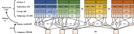
In order to map patent pieces to technologies, we utilize the widely used Cooperative Patent Classification (CPC). In fact, CPC is a patent classification system, which has been jointly developed by the European Patent Office (EPO) and the USPTO. As shown in Fig. 1, CPC has four levels. From the top down, technology categories are partitioned more and more detailed. For example, the first level ’section’ has 9 classifications, and the code ’H’ represents ’Electricity’; the third level has 662 classifications and ’H04J’ means ’Multiplex Communication’. In general, each US patent is allocated several CPC codes according to their involved technologies at the beginning of its application. Therefore, given a company, we can find all its applied or granted patents as well as their corresponding technologies represented by CPC codes.

II-B Statistics on Companies and Technologies

In this part, we give some data statistics for revealing several supportive observations of companies and technologies.

Figure 2: The technology evolving trend of Apple Inc. from 2000 to 2015.

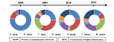
Fig. 2 depicts the evolving trend of 7 typical technologies of Apple Inc. from 2000 to 2015. Here we can see it is continually changing with time: some technologies keep increasing while some decreasing, i.e., the growing ’H04W’ and the shrinking ’H04L’. It may tell the development trend that ’H04W’ acts as Apple’s current technology emphasizes and may potentially keep increasing in the next few years.

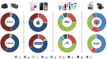
Then, we analyze the technology distribution (based on CPC section) of different types of companies shown in Fig. 3, from which we have three observations:

Figure 3: Technology distribution of different types of companies.

• Each company has its own technical strengths and weaknesses, indicated by the varying proportions of different technologies. For example, the Procter & Gamble Company shows a great advantage in technology ’C’ (Chemistry), while a disadvantage in technology ’G’ (Physics).

• Companies who tend to be competitors share similar technology distributions. For instance, the top 3 technology categories of both Apple and Samsung are ’G’ (Physics), ’H’ (Electricity) and ’B’ (Performing Operations; Transporting).

• Technology distributions among different types of companies vary a lot, which can be easily found from any two columns of Fig. 3.

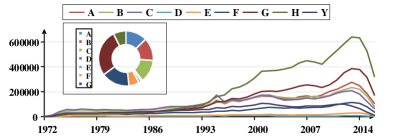
Fig. 4 shows the number of patents granted in different CPC sections from 1972 to 2016. Here we can see a booming increase of most technologies, and the growth of some technologies seems kind of synchronous. For example, section ’H’ (Electricity) and ’G’ (Physics) have a very similar trend, which might benefit by the rapid development of the information industry, especially electronic hardwares like semiconductors.

Figure 4: Technology evolving trend from 1972 to 2016 based on CPC section.

Figure 5: Overall Architecture of Deep Technology Forecasting (DTF) Framework.

The above interesting observations can be instructive and meaningful, from which we can summarize following instructions for predicting the R&D directions of a given company:

• Internal and external factors. When predicting the R&D directions of a given company, we need to consider both internal factors, i.e., its original technical strengths and weaknesses, and external factors, i.e., the development trend of technologies in overall market place.

• Relations among companies and technologies. Competitive relations among companies and collaborative relations among technologies can be also a great help.

• Dynamics of companies and technologies. Both the companies and technologies keep evolving consistently, so we need also to model the dynamic interactions among them.

III Problem Statement

Suppose there are $\small M$ companies ($\small{U={U_{i}|i=1,2,\cdots,M}}$), $\small N$ technologies ($\small V={V_{j}|j=1,2,\cdots,N}$) and $\small Q$ patents ($\small P={P_{k}|k=1,2,\cdots,Q}$) within $T$ years in patent database. Then, for company $\small U_{i}\in U$, its patent filing history can be represented by $\small{S_{U_{i}}=[S_{U_{i}^{1}},S_{U_{i}^{2}},\cdots,S_{U_{i}^{t}},\cdots,S_{U_{i}^{T}}]}$, where $\small S_{U_{i}^{t}}$ indicates the set of patents that $\small U_{i}$ files in year $t$. Similarly, for technology $\small V_{j}\in V$, its patent filing records can also be denoted as $\small{S_{V_{j}}=[S_{V_{j}^{1}},S_{V_{j}^{2}},\cdots,S_{V_{j}^{t}},\cdots,S_{V_{j}^{T}}]}$, where $\small S_{V_{j}^{t}}$ indicates the set of patents filed in year $t$ belonging to $\small V_{j}$. Specifically, technology distribution of $\small U_{i}\in U$ in year $t$ is defined as:

$$\begin{array}[]{l}{\small r_{i}^{t}=[r_{i,1}^{t},r_{i,2}^{t},\cdots,r_{i,j}^{t},\cdots,r_{i,N}^{t}]},\\ {\small r_{i,j}^{t}=\frac{|S_{U_{i}^{t}}\cap S_{V_{j}^{t}}|}{|S_{U_{i}^{t}}|}},\\ \end{array}$$ (1)

where $\small{|S_{U^{t}_{i}}\cap S_{V^{t}_{j}}|}$ means the number of patents belonging to $\small V_{j}$ that $\small U_{i}$ files in year $t$. Obviously, if $U_{i}$ files a large number of patents belonging to $\small V_{j}$ in year $t$, we will have a big $\small r_{i,j}^{t}$, indicating that $\small U_{i}$ pays a great emphasis on $\small V_{j}$ in year $t$.

Then we can formalize our research problem as follows: Given the patent filing history of a company $\small U_{i}$ before year $\small T$, $\small{S_{U_{i}}=[S_{U^{1}_{i}},S_{U^{2}_{i}},\cdots,S_{U^{T-1}_{i}}]}$, and that of a technology $\small V_{j}$, $\small{S_{V_{j}}=[S_{V^{1}_{j}},S_{V^{2}_{j}},\cdots,S_{V^{T-1}_{j}}]}$, our goal is to predict $r_{i,j}^{T}$, and thus the whole technology distribution of $\small U_{i}$ in year $\small T$, represented by $\small{r_{i}^{T}=[r_{i,1}^{T},r_{i,2}^{T},\cdots,r_{i,N}^{T}]}$.

Figure 6: The architecture of Deep Technology Tracing (DTT) Neural Network.

IV DTF Framework

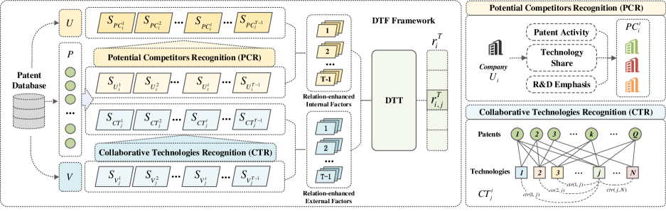
In this section, we provide a possible solution to the technology tracing problem, i.e., Deep Technology Forecasting (DTF) framework shown in Fig. 5, including Potential Competitors Recognition (PCR), Collaborative Technology Recognition (CTR), and Deep Technology Tracing (DTT) neural network.

IV-A Potential Competitors Recognition (PCR)

Given a company $\small U_{i}\in U$, PCR aims to find its most likely competitors $\small PC_{i}^{t}\subset U$ in year $t$. Inspired by [3], we apply three commonly used patent indicators for evaluating competitions among companies:

• Patent Activity ($\small I_{1}=|S_{U_{i}^{t}}\cap S_{V_{j}^{t}}|$) is a fundamental patenting indicator. Decreasing or increasing of $I_{1}$ can be interpreted as changing levels of R&D activity, and therefore, future technological and commercial [3].

• Technology Share ($\small I_{2}={|S_{U_{i}^{t}}\cap S_{V_{j}^{t}}|}/{|S_{V_{j}^{t}}|}$) is based on patent applications, which measures a firm’s competitive position in a technological field.

• R&D Emphasis ($\small I_{3}={|S_{U_{i}^{t}}\cap S_{V_{j}^{t}}|}/{|S_{U_{i}^{t}}|}$) illustrates the importance placed on a specific technological field within a firm’s entire R&D portfolio.

Then, we develop a competitive score for measuring competitive degrees based on the commonly used Euclidean distance. Specially, for $\small U_{i_{1}}\in U$ and $\small U_{i_{2}}\in U$ in year $t$, the competitive degree between them are denoted as:

$$\small pcr^{t}(U_{i_{1}},U_{i_{2}})=\sqrt{\sum_{q=1}^{3}\alpha_{q}(I_{q}^{U_{i_{1}},t}-I_{q}^{U_{i_{2}},t})^{2}},\\$$ (2)

where $\small I_{q}^{U_{i_{1}},t}$, $\small I_{q}^{U_{i_{2}},t}$ represents the $q$th indicator of $\small U_{i_{1}}$ and $\small U_{i_{2}}$ in year $t$ respectively, and $\alpha_{q}$ is the corresponding weight of $\small I_{q}$. Through Eq.2, given $\small U_{i}\in U$ in year $t$, we can rank and get its top-$m$ potential competitors, indicated by $\small PC_{i}^{t}$.

IV-B Collaborative Technology Recognition (CTR)

As shown in Fig. 5, for each year, we first construct a bipartite whose nodes are patents and technologies while edges represent the ownership between them. In detail, if $\small P_{k}\in P$ belongs to $\small V_{j}\in V$, there will be an edge connecting $\small P_{k}$ and $\small V_{j}$. Then, a weighted network can be established, whose nodes are technologies and edges are their collaborations. Here, weight of edge between $\small V_{j_{1}}$ and $\small V_{j_{2}}$ is calculated by:

$$\small ctr^{t}(V_{j_{1}},V_{j_{2}})={|S_{V_{j_{1}}^{t}}\cap S_{V_{j_{2}}^{t}}|}/{|S_{V_{j_{1}}^{t}}\cup S_{V_{j_{2}}^{t}}|},\\$$ (3)

where $\small{|S_{V_{j_{1}}^{t}}\cap S_{V_{j_{2}}^{t}}|}$ means the number of common patents shared by $\small V_{j_{1}}$ and $\small V_{j_{2}}$ in year $t$, and $\small{|S_{V_{j_{1}}^{t}}\cup S_{V_{j_{2}}^{t}}|}$ represents the total number of patents filed in $\small V_{j_{1}}$ and $\small V_{j_{2}}$ in year $t$. Naturally, bigger $\small ctr^{t}(V_{j_{1}},V_{j_{2}})$ indicates a deeper collaboration. In this way, given $\small V_{j}\in V$ in year $t$, we can rank and get its top-$n$ collaborations, indicated by $\small CT_{j}^{t}$.

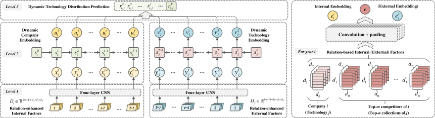
IV-C Deep Technology Tracing (DTT) Neural Network

Fig. 6 shows architecture of Deep Technology Tracing (DTT) Neural Network, which can be partitioned into three levels: 1) relation-enhanced factor representation; 2) dynamic embedding for companies and technologies; 3) final prediction for a given company and technology.

IV-C1 Relation-enhanced Factor Representation

As the first level of DTT, this part aims at learning the semantic representation of relation-enhanced internal and external factors.

As shown in the right part of Fig. 6, each patent is combined with a sequence of words $e=[e_{1},{e}_{2},\cdots,{e}_{d1}]$, where ${e}_{i}\in\mathbb{R}^{d_{0}}$ is initialized by $d_{0}$-dimensional pre-trained word embedding and $d_{1}$ is the length of ${e}$. Then, for each company in each year, we totally sample $d_{2}$ patents as its internal factors. Then, patents of one company can be depicted by a tensor ${D}\in\mathbb{R}^{d_{2}*d_{1}*d_{0}}$. With the top-$m$ competitors extracted by PCR, we totally get $m+1$ company tensors in each year. In this way, relation-enhanced internal factors of company $\small U_{i}$ can be represented by $\small{D}_{i}\in\mathbb{R}^{(m+1)*d_{2}*d_{1}*d_{0}}$. Similar operations are applied in external factor extraction, so we also have $\small{D}_{j}\in\mathbb{R}^{(n+1)*d_{2}*d_{1}*d_{0}}$, i.e. the relation-enhanced external factor tensor in each year.

Next, we try to transform the above $\small{D}_{i}$ and $\small{D}_{j}$ into lower semantic embeddings through the commonly used convolutional neural network (CNN) [8]. Three layers of convolution-pooling processes are set to gradually summarize the global interactions of words in a patent and finally reach a vectorial representation one $\dot{{e}}\in\mathbb{R}^{d}$, where $d$ is the output dimension of one patent document. Thus, company $i$ who have $d_{2}$ patents in each year can be represented as ${a}_{i}=\sigma({\dot{{e}}_{1},\dot{{e}}_{2},\cdots,\dot{{e}}_{d_{2}}})$, where ${a}_{i}\in\mathbb{R}^{d}$ and $\sigma$ is a mean value function. Along this line, the relation based internal factor tensor $\small{D}_{i}\in\mathbb{R}^{(m+1)*d_{2}*d_{1}*d_{0}}$ can be transformed into $\small{D}_{i}\in\mathbb{R}^{(m+1)*d}$.

So, the relation-enhanced internal factor embedding of company $\small U_{i}$ in year $t$ is given by Eq. (4), where $\small pcr^{t}(U_{i},U_{i^{\prime}})$ is the competition score calculated in PCR, and ${a}_{i}^{t}\in\mathbb{R}^{d}$ is the patent embedding of $\small U_{i}$ in year $t$.

$$\small{x}_{i}^{t}={a}_{i}^{t}+\sum_{i^{\prime}\in PC_{i}^{t}}pcr^{t}(U_{i},U_{i^{\prime}})*{a}_{i^{\prime}}^{t}.\\$$ (4)

Similarly, the relation-enhanced external factor embedding of technology $j$ in year $t$ is given by Eq. (5), where $\small ctr^{t}(V_{j},V_{j^{\prime}})$ is the collaborative score calculated in CTR, and ${a}_{j}^{t}\in\mathbb{R}^{d}$ is the patent latent embedding of $\small V_{j}$ in year $t$.

$$\small{y}_{j}^{t}={a}_{j}^{t}+\sum_{j^{\prime}\in CT_{j}^{t}}ctr^{t}(V_{j},V_{j^{\prime}})*{a}_{j^{\prime}}^{t}.\\$$ (5)

IV-C2 Dynamic Embedding for Companies & Technologies

We employ Gated Recurrent Unit (GRU) [9] to model the dynamic interactions of companies and technologies. As depicted in Fig. 6, given the yearly internal factor embedding sequence of company $\small U_{i}$, i.e., $\small{{x}_{i}=\{{x}_{i}^{1},{x}_{i}^{2},\cdots,{x}_{i}^{T-1}\}}$, GRU updates the cell vector sequence $\small{{s}_{i}=\{{s}_{i}^{1},{s}_{i}^{2},\cdots,{s}_{i}^{T-1}\}}$ and company hidden state $\small{{u}_{i}=\{{u}_{i}^{2},{u}_{i}^{3},\cdots,{u}_{i}^{T}\}}$ from $t=1$ to $t=T-1$. After the initialization, in year $t$, the company state ${u}_{i}^{t+1}$ is updated by the previous hidden state ${u}_{i}^{t}$ and the current internal embedding vector ${x}_{i}^{t}$, which is shown as:

$$\small\begin{array}[]{l}{\bm{z}_{i}^{t+1}=\sigma\left({W}_{xz}{x}_{i}^{t+1}+{W}_{uz}{u}_{i}^{t}\right)}\\ {{r}_{i}^{t+1}=\sigma\left({W}_{xr}{x}_{i}^{t+1}+{W}_{ur}{u}_{i}^{t}\right)}\\ {\tilde{{u}}_{i}^{t+1}=\tanh\left({W}_{xu}{x}_{i}^{t+1}+{r}_{i}^{t+1}\odot\left({W}_{uu}{u}_{i}^{t}\right)\right)}\\ {{u}_{i}^{t+1}=\left(\mathbf{1}-{z}_{i}^{t+1}\right)\odot\tilde{{u}}_{i}^{t+1}+{z}_{i}^{t+1}\odot{u}_{i}^{t}}\end{array},\\$$ (6)

where ${z}_{i}^{t+1}$, ${r}_{i}^{t+1}$ are the update and reset gate, respectively. $\odot$ is an element-wise multiplication and $\sigma$ is non-linear activation function which is stated as sigmoid in this paper. ${W}_{*}$ denotes weight matrices, which are all optimized in training process. In this way, the whole evolving process of $\small U_{i}$ in year $t$ are embedded into a hidden embedding state ${u}_{i}^{t+1}$, in different years integrated by different relation-enhanced internal embeddings.

Similar operations are done for mining dynamics of technologies. Then, the final latent embedding ${v}_{j}^{t+1}$ of $\small V_{j}$ in year $t$ is also captured automatically, in different years referring to different relation-enhanced external embedding.

IV-C3 Technology Distribution Forecasting

After the above modules, we acquire the latent embeddings of companies and technologies from year $1$ to $T$, denoted by $\small{u^{t}=[u_{1}^{t},u_{2}^{t},\cdots,u_{M}^{t}]}$ and $\small{v^{t}=[v_{1}^{t},v_{2}^{t},\cdots,v_{N}^{t}]}$. Then, when making predictions, we feed ${u}$ and ${v}$ into a function, $\small\hat{r}_{uv}=\mathcal{P}({u},{v})$, where $\mathcal{P}$ is an arbitrary prediction function or a prediction neural network. For the sake of simplicity, we set $\hat{r}_{uv}=\sigma({u}\cdot{v})$, which is more efficient for training and easier to avoid overfitting, and $\sigma$ is a sigmoid function.

Specially, we adopt the idea of Bayesian Personalized Ranking (BPR) [10] for pair-wise learning, which has been widely used in recommendation tasks:

$$\small L=\sum_{(i,j)\in\mathcal{D}_{S}}-\ln\sigma(\hat{r}_{ij^{+}}-\hat{r}_{ij^{-}})+\lambda||\Theta||^{2},$$ (7)

where $\Theta$ includes all model parameters, and $\lambda$ and is the regularization factor. $\mathcal{D}_{S}$ indicates the whole training set, which consists of many triples in form of $(i,j^{+},j^{-})$, meaning that company $i$ shows a greater emphasis on technology $j^{+}$ than $j^{-}$. In order to minimize the above object function, we adopt Adadelta optimizer [11] to update the model parameters with back propagation algorithm, which can be implemented automatically through Tensorflow.

V Experiment

In this section, extensive experiments are conducted on USPTO patent dataset to verify the effectiveness of Deep Technology Forecasting framework.

V-A Experimental Settings

The USPTO dataset includes 6,014,932 granted US patents from 1972 to 2017, belonging to 389,246 patent assignees. After cleaning, we totally get 2,791 high-tech companies, who have filed at least 200 patents since 1972. In addition, all experiments are conducted based on CPC group, meaning that we aim to make predictions on 662 pre-defined technologies.

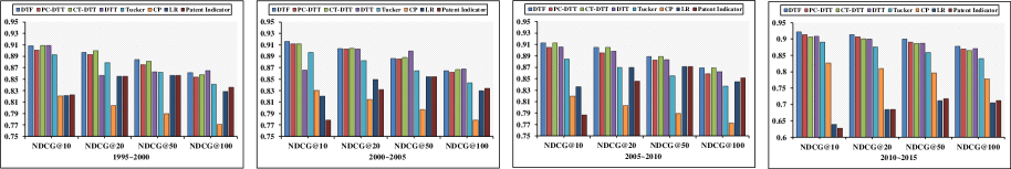
For better proving the effectiveness of DTF framework, we divide the patent dataset from 1995 to 2015 into four periods, on which experiments are made separately. Let’s take 1995 to 2000 as an example. In training stage, we apply patent filing histories of companies and technologies from 1995 to 1999 as input, and technology distribution in 2000 as a ground truth. For testing, one year is shifted backwards, i.e. with data from 1996 to 2000 as input and 2011 as the prediction target. Treating it as a ranking problem, we evaluate the performance of DTF by the Normalized Discounted Cumulative Gain ($NDCG@K$, $K=10,20,50,100$). All experiments are implemented on a Linux server with four 2.0GHz Intel Xeon E5-2620 CPUs and a Tesla K20m GPU.

Figure 7: The experimental results on four datasets.

TABLE I: A Case study on Hughes Net-work Systems, LLC

Methods	Predicted Top@10 Technologies
Ground Truth	H04L	H04W	H04B	H03M	H03H	G06F	H04M	H01Q	G06E	A44B
DTF	H04L	H04W	H04B	H03M	H04M	G10C	H04Q	B60G	Y02W	G09F
PC-DTT	H04L	H04W	H04B	H03M	C12Q	G10D	B60G	F02C	F16M	H04M
CT-DTT	H04L	H04W	H04B	H03M	G06F	D02H	G06C	E21B	H04Q	C12P
DTT	H04L	H04W	H04B	H03M	C23F	D06C	Y10T	C22B	H04J	F42D

Codes	Meanings
H04L	Transmission of digital information
H04W	Wireless communication networks
H04B	Transmission systems
H03M	Coding; Decoding; Code conversion
H03H	Impedance networks

V-B Compared Methods

Since there are few prior works to directly predict the possible technologies customized to companies’ personalized R&D needs, we introduce some variants of DTF to highlight the effectiveness of each component of our framework.

• PC-DTT excludes the collaborative relations among technologies as the input of DTT.

• CT-DTT excludes the competitve relations among technologies as the input of DTT.

• DTT only inputs the patent filing history of companies and technologies as well as their dynamic interactions.

• CP [12] only models the dynamic interactions between companies and technologies.

• Tucker [13] has the same settings with CP.

• LR ignores the dynamic embeddings of companies and technologies.

• Patent Indicator [14] can also give useful advice for predicting emerging technologies in special technology fields.

V-C Experimental Results

Fig. 7 shows the performances of DTF and compared methods within four time periods. Here, we can observe that in most cases DTF performs much better than baselines under all metrics with respect to different $K$, indicating that it is meaningful to integrate both the relation-enhanced internal and external factors along with dynamic interactions among companies and technologies.

Among DTF and its variants, DTF often performs best, proving the effectiveness of competitions extracted by PCR and collaborations extracted by CTR. What’s more, there seems a tight race between PC-DTT and CT-DTT: on the first three datasets, CT-DTT shows a great advantage beyond PC-DTT, while on the last one, CT-DTT behaves much better than CT-DTT. This phenomenon may indicate that competitive relations among companies have gradually become more and more important for technology tracing.

Compared with baselines including Tucker, CP and LR, DTF still behaves better. For one thing, although Tucker and CP model the same dynamic interactions, they yet do not perform very well, which proves that patent content information can be very useful for mining technology distribution. For another, LR integrates the yearly content information the same as DTF while shows a bed performance, especially when $K$ is set as 10 and 20, indicating the fact that dynamic interactions among companies and technologies can not be ignored.

In the end, almost all models behave better from 1999 to 2010 except for Patent Indicator, which is understandable in that patents filed in recent years haven’t received many citations, so statistics-based Patent Indicators have no access to distinctive features (especially citation-based features). However, DTF shows an advantage in this term, because it tries to learn potential semantic information from many patent documents, depending less on statistics-based features.

V-D Case Study.

In this section, we present a case study on Hughes Network Systems, LLC (Hughes), which is the global leader in broadband satellite technology and services for home and office. Table I shows top 10 technologies in 2016 of Hughes predicted by DTF and its variants. From this table, we can see that both DTF and its variants successfuly predict LLC (Hughes) will pay the most emphasis on technologies about network communication, represented by CPC codes as ’H04L’, ’H04W’, ’H04B’, and ’H03M’. However, about the followings, they have very different ideas: 1) Both DTF and PC-DTT prefer ’B60G’ (Vehicle suspension arrangements), which may give a signal that its competitors may have some businesses in this field; 2) Both DTF and CT-DTT think ’H04Q’ (switches, relays etc.) will be an important technology for Hughes, which might be due to the big collaboration degrees with the former technologies, especially ’H04W’. In fact, they share 39,898 common patents according to our statistics.

VI Related Work

Patent data has been widely explored for decision-making processes and strategic planning purposes [3, 4, 5]. Typically, methods related to technology prospecting can be summarized as two types: qualitative analysis and quantitative mining. Qualitative approaches are mainly based on analysis by domain experts, which naturally needs many human efforts, and in addition, some researches [15] find that these subjective strategies may be not always precisely correct and reliable. Quantified approaches aim to access potential prospects of technologies through supervised machine learning methods [14, 5].

Nowadays, deep learning has been widely used in many traditional areas, i.e. education [16], financial analyses [17], music generation [18], patent mining [7], and etc. In particular, Recurrent Neural Networks (RNN) are powerful tools for modeling sequences, which are flexibly extensible and can incorporate various kinds of information including temporal order [19]. Its variants, such as Long Short-Term Memory (LSTM) [20] and Gated Recurrent Unit (GRU) [9], have capability to model dependency among sequences.

VII Conclusion and Future Work

In this paper, we presented a focused study on technology tracing problem. Specifically, we designed a novel data-driven Deep Technology Forecasting (DTF) framework including three components: Potential Competitor Recognition (PCR), Collaborative Technology Recognition (CTR), and Deep Technology Tracing (DTT) neural network. For one thing, PCR aimed to capture the competitive relations among enterprises and CTR tried to figure out the collaborative relations among technologies. For another, DTT targeted at modeling dynamic interactions between companies and technologies. Finally, we evaluated our DTF framework on real-world patent data and the experimental results clearly proved its effectiveness. We hope this work could lead to more future studies.

VIII Acknowledgements

This research was partially supported by grants from the National Key Research and Development Program of China (No. 2018YFC0832101), the National Natural Science Foundation of China (Grants No., 61672483, 61727809), the Young Elite Scientist Sponsorship Program of CAST and the Youth Innovation Promotion Association of CAS (No. 2014299).

References

- [1] Jenő Kürtössy. Innovation indicators derived from patent data. Periodica Polytechnica Social and Management Sciences, 12(1):91–101, 2004.
- [2] Youngjin Park and Janghyeok Yoon. Application technology opportunity discovery from technology portfolios: Use of patent classification and collaborative filtering. Technological Forecasting and Social Change, 118:170–183, 2017.
- [3] Holger Ernst. Patent information for strategic technology management. World patent information, 25(3):233–242, 2003.
- [4] Gabjo Kim and Jinwoo Bae. A novel approach to forecast promising technology through patent analysis. TFSC, 117:228–237, 2017.
- [5] Péter Érdi, Kinga Makovi, Zoltán Somogyvári, Katherine Strandburg, Jan Tobochnik, Péter Volf, and László Zalányi. Prediction of emerging technologies based on analysis of the us patent citation network. Scientometrics, 95(1):225–242, 2013.
- [6] Jesus Galende Del Canto and Isabel Suarez Gonzalez. A resource-based analysis of the factors determining a firm’s r&d activities. Research Policy, 28(8):891–905, 1999.
- [7] Qi Liu, Han Wu, Yuyang Ye, Hongke Zhao, Chuanren Liu, and Dongfang Du. Patent litigation prediction: A convolutional tensor factorization approach. In IJCAI, pages 5052–5059, 2018.
- [8] Yoav Goldberg. A primer on neural network models for natural language processing. J. Artif. Intell. Res.(JAIR), 57:345–420, 2016.
- [9] Kyunghyun Cho, Bart Van Merriënboer, Dzmitry Bahdanau, and Yoshua Bengio. On the properties of neural machine translation: Encoder-decoder approaches. arXiv preprint arXiv:1409.1259, 2014.
- [10] Steffen Rendle, Christoph Freudenthaler, Zeno Gantner, and Lars Schmidt-Thieme. Bpr: Bayesian personalized ranking from implicit feedback. In UAI, pages 452–461. AUAI Press, 2009.
- [11] Matthew D Zeiler. Adadelta: an adaptive learning rate method. arXiv preprint arXiv:1212.5701, 2012.
- [12] Tamara G Kolda and Brett W Bader. Tensor decompositions and applications. SIAM review, 51(3):455–500, 2009.
- [13] Lieven De Lathauwer, Bart De Moor, and Joos Vandewalle. A multilinear singular value decomposition. SIAM journal on Matrix Analysis and Applications, 21(4):1253–1278, 2000.
- [14] Moses Ntanda Kyebambe, Ge Cheng, Yunqing Huang, Chunhui He, and Zhenyu Zhang. Forecasting emerging technologies: A supervised learning approach through patent analysis. Technological Forecasting and Social Change, 125:236–244, 2017.
- [15] Jeongjin Lee, Changseok Kim, and Juneseuk Shin. Technology opportunity discovery to r&d planning: Key technological performance analysis. Technological Forecasting and Social Change, 119:53–63, 2017.
- [16] Zhenya Huang, Yu Yin, Enhong Chen, Hui Xiong, Yu Su, Guoping Hu, et al. Ekt: Exercise-aware knowledge tracing for student performance prediction. IEEE TKDE, 2019.
- [17] Liang Zhang, Keli Xiao, Hengshu Zhu, Chuanren Liu, Jingyuan Yang, and Bo Jin. Caden: A context-aware deep embedding network for financial opinions mining. In IEEE ICDM, pages 757–766. IEEE, 2018.
- [18] Hongyuan Zhu, Qi Liu, Nicholas Jing Yuan, Chuan Qin, Jiawei Li, Kun Zhang, Guang Zhou, Furu Wei, Yuanchun Xu, and Enhong Chen. Xiaoice band: A melody and arrangement generation framework for pop music. In SIGKDD, pages 2837–2846. ACM, 2018.
- [19] Tim Donkers, Benedikt Loepp, and Jürgen Ziegler. Sequential user-based recurrent neural network recommendations. In Proceedings of the Eleventh ACM Conference on Recommender Systems, pages 152–160. ACM, 2017.
- [20] Alex Graves, Abdel-rahman Mohamed, and Geoffrey Hinton. Speech recognition with deep recurrent neural networks. In 2013 IEEE international conference on acoustics, speech and signal processing, pages 6645–6649. IEEE, 2013.