Learning Distributional Programs for Relational Autocompletion

Abstract

Relational autocompletion is the problem of automatically filling out some missing values in multi-relational data. We tackle this problem within the probabilistic logic programming framework of Distributional Clauses (DC), which supports both discrete and continuous probability distributions. Within this framework, we introduce DiceML – an approach to learn both the structure and the parameters of DC programs from relational data (with possibly missing data). To realize this, DiceML integrates statistical modeling and distributional clauses with rule learning. The distinguishing features of DiceML are that it 1) tackles autocompletion in relational data, 2) learns distributional clauses extended with statistical models, 3) deals with both discrete and continuous distributions, 4) can exploit background knowledge, and 5) uses an expectation-maximization based algorithm to cope with missing data. The empirical results show the promise of the approach, even when there is missing data.

1 Introduction

Spreadsheets are arguably the most accessible tool for data analysis and millions of users use them. Generally, real-world data is not gathered in a single table but in multiple tables that are related to each other. Real-world data is often noisy and may have missing values. End users, however, do not have access to the state-of-the-art techniques offered by Statistical Relational AI (StarAI, Kersting et al., 2011) to analyze such data. To tackle this issue, we study the problem of relational autocompletion, where the goal is to automatically fill out the entries specified by users in multiple related tables. This problem setting is simple, yet challenging and is viewed as an essential component of an automatic data scientist (De Raedt et al., 2018). We tackle this problem by learning a probabilistic logic program that defines the joint probability distribution over attributes of all instances in the multiple related tables. This program can then be used to estimate the most likely values of the cells of interest.

Probabilistic logic programming (PLP, Ngo and Haddawy, 1997; Sato, 1997; Vennekens et al., 2004; De Raedt et al., 2007; Poole, 2008) and statistical relational learning (SRL, Jaeger, 1997; Richardson and Domingos, 2006; Koller et al., 2007; Natarajan et al., 2008; Neville and Jensen, 2007; Kimmig et al., 2012) have introduced various formalisms that integrate relational logic with graphical models. While many PLP and SRL techniques exist, only a few of them are hybrid, i.e., can deal with both discrete and continuous variables. One of these hybrid formalisms are the Distributional Clauses (DC) introduced by Gutmann et al. (2011). Distributional clauses form a probabilistic logic programming language that extends the programming language Prolog with continuous as well as discrete probability distributions. It is this language that we adopt in this paper.

We first integrate statistical models in distributional clauses and use these to learn intricate patterns present in the data. This extended DC framework allows us to learn a DC program that specifies a probability distribution over attributes of multiple tables. Just like graphical models, this program can then be used for various types of inference. For instance, one can infer not only the output of statistical models based on their inputs but also the input when the output is observed.

In line with inductive logic programming (Muggleton, 1991; Lavrac and Dzeroski, 1994; Quinlan and Cameron-Jones, 1995), we propose an approach, named DiceML  (Distributional Clauses with Statistical Models Learner), that learns such a DC program from relational data and background knowledge. DiceML jointly learns the structure of distributional clauses, the parameters of its probability distributions and the parameters of the statistical models. The learned program can subsequently be used for autocompletion.

We study the problem also in the presence of missing data. The problem of learning the structure of hybrid relational models then becomes even more challenging and has, to the best of our knowledge, never been attempted before. To tackle this problem, DiceML performs structure learning inside the stochastic EM procedure (Diebolt and Ip, 1995).

Related Work

There are several works in SRL for learning probabilistic models for relational data, such as probabilistic relational models (PRMs, Friedman et al., 1999), relational Markov networks (RMNs, Taskar et al., 2002), and relational dependency networks (RDNs, Neville and Jensen, 2007). PRMs extend Bayesian networks with concepts of objects, their properties, and relations between them. RDNs extend dependency networks, and RMNs extend Markov networks in the same relational setting. However, these models are generally restricted to discrete data. To address this shortcoming, several hybrid SRL formalisms were proposed such as continuous Bayesian logic programs (CBLPs, Kersting and De Raedt, 2007), hybrid Markov logic networks (HMLNs, Wang and Domingos, 2008), hybrid probabilistic relational models (HPRMs, Narman et al., 2010), and relational continuous models (RCMs, Choi et al., 2010). The work on hybrid SRL has mainly been focused on developing theory to represent continuous variables within the various SRL formalisms and on adapting inference procedures for hybrid domains. However, little attention has been given to the design of algorithms for structure learning of hybrid SRL models. The same is true for works on hybrid probabilistic programming (HProbLog, Gutmann et al., 2010), (DC, Gutmann et al., 2011; Nitti et al., 2016), (Extended-Prism, Islam et al., 2012), (Hybrid-cplint, Alberti et al., 2017), (Michels et al., 2016), (BLOG, Wu et al., 2018), (Dos Martires et al., 2019). Closest to our work is the work on hybrid relational dependency networks (HRDNs, Ravkic et al., 2015), for which structure learning was also studied, but this learning algorithm assumes that the data is fully observed. There are also few approaches for structure learning in the presence of missing data such as Kersting and Raiko (2005); Khot et al. (2012, 2015). However, these approaches are restricted to discrete data. Furthermore, existing hybrid models that extend probabilistic graphical models with relations, such as HRDNs, are associated with local probability distributions such as conditional probability tables. As a result, it is difficult to represent certain independencies such as context-specific independencies (CSIs, Boutilier et al., 1996). On the contrary, DC can represent CSIs leading to interpretable DC programs.

Learning meaningful and interpretable symbolic representations from data in the form of rules has been studied in many forms by the inductive logic programming(ILP) community (Quinlan, 1990; Muggleton, 1995; Blockeel and De Raedt, 1998; Srinivasan, 2001). The standard ILP setting requires the input to be deterministic and usually the rules as well. Although some rule learners (Neville et al., 2003; Vens et al., 2007) output the confidence of their predictions, the rules learned for different targets have not been used jointly for probabilistic inference. To alleviate these limitations, De Raedt et al. (2015) proposed ProbFoil+ that can learn probabilistic rules from probabilistic data and background knowledge. In this approach, rules learned for different targets can jointly be used for inference. However, this approach does not deal with continuous random variables and missing data. A handful approaches can learn rules with continuous probability distributions, and the learned rules can also be jointly used for inference. One such approach was proposed by Speichert and Belle (2018) using piecewise polynomials to learn intricate patterns from data. This approach differs from our approach as we use statistical models to learn these patterns. Moreover, it is restricted to fully observed deterministic input. Another approach for structure learning of dynamic distributional clauses, an extended DC framework that deals with time, has also been proposed by Nitti et al. (2016). However, this approach cannot learn distributional clauses from background knowledge, which itself can be a set of distributional clauses. Furthermore, it learns the dynamic distributional clauses from fully observed data and does not deal with missing values in relational data as we do. To the best of our knowledge, the present paper makes the first attempt to learn interpretable hybrid probabilistic logic programs from partially observed probabilistic data as well as background knowledge. DC programs have been successfully applied in robotics and perceptual anchoring using handcrafted programs or by learning parameters of simple programs with defined structure (Moldovan et al., 2018; Persson et al., 2019). The technique we present in the present paper has already been successfully applied for structure learning in the perceptual anchoring context (Zuidberg Dos Martires et al., 2020) and extends these other results.

Our approach also deals with missing values in relational data. Thus, it is also related to the vast literature on database cleaning (Ilyas and Chu, 2015). However, there are not many database-cleaning methods that can learn distributions of the data and use them to automatically fill in missing data (mostly due to the complexity of the problem and the scale of real-world relational databases), and those methods that can to some extent model probability distributions, e.g. (Yakout et al., 2013; Rekatsinas et al., 2017), still cannot model complex probability distributions involving both discrete and continuous random variables. While the approach presented in this paper cannot scale to databases containing billions of tuples, it can model very complex probabilistic distributions.

A different approach for autocompletion in spreadsheets was proposed by Kolb et al. (2020). In this approach, multiple related tables are joined in a pre-processing step in order to obtain a single table, and then constraints and Bayesian networks are learned. Thus this approach propositionalizes the data, which implies that the joined table may contain redundant information, implying that the learned model will not be succinct. Learning succinct first-order probabilistic models, which we do, is required to truly deal with relational data.

Contributions

We summarise our contributions in this paper as follows:

• We integrate distributional clauses with statistical models and use the resulting framework to represent a hybrid probabilistic relational model.

• We introduce DiceML, the approach for relational autocompletion that learns distributional clauses with statistical models from relational data and background knowledge.

• We extend DiceML to learn DC programs from relational data with missing values using the stochastic EM algorithm.

• We empirically evaluate DiceML on synthetic as well as real-world data, which shows the promise of our approach.

Organization

The paper is organized as follows. We start by sketching the problem setting in Section 2. Section 3 reviews logic programming concepts and distributional clauses. In Section 4, we discuss the integration of distributional clauses with statistical models. In Section 5, we describe the specification of the DC program that we shall learn. Section 6.1 explains the learning algorithm, which is then evaluated in Section 7.

2 Problem Setting

Let us introduce relational autocompletion using the simplified spreadsheet in Table 1. It consists of entity tables and associative tables. Each entity table (e.g., client, loan, and account) contains information about instances of the same type. An associative table (e.g., hasAcc and hasLoan) encodes a relationship among entities. This toy example illustrates two important properties of real-world applications, namely i) the attributes of entities may be numeric or categorical, and ii) there may be missing values in entity tables. These are denoted by “$-$”.

In addition, certain knowledge is available beforehand, and inclusion of this background knowledge might be useful for learning; for instance, if a client of a bank has an account, and the account is linked to a loan, then the client has the loan. Knowledge may even be uncertain; for instance, we might already have a probabilistic model that specifies a probability distribution over the age of clients.

The problem that we tackle in this paper is to autocomplete specific cells selected by users, denoted by “$?$”. This problem will be solved by automatically learning a DC program from such data and background knowledge. This program can then be used to fill out those cells with the most likely values. This setting can be viewed as a simple nontrivial setting for automating data science (De Raedt et al., 2018).

client
cliId	age	creditScore
ann	33	$-$
bob	40	500
carl	$-$	450
john	55	700

hasAcc
cliId	accId
ann	a_11
bob	a_11
ann	a_20
john	a_10

hasLoan
accId	loanId
a_11	l_20
a_10	l_20
a_20	l_31
a_20	l_41

loan
loanId	loanAmt	status
l_20	20050	appr
l_21	$-$	pend
l_31	25000	decl
l_41	10000	$-$

account
accId	savings	freq
a_10	3050	high
a_11	$-$	low
a_19	3010	$?$
a_20	$?$	$?$

Table 1: An example of a spreadsheet consisting of entity tables (client, loan and account), and associative tables (hasLoan and hasAcc). Missing cells are denoted by “$-$” and the cells of interest are denoted by “$?$”.

3 Probabilistic Logic Programming

In this section, we first briefly review logic programming concepts and then introduce DC which extend logic programs with probability distributions.

3.1 Logic Programming

An atom $p(t_{1},\dots,t_{n})$ consists of a predicate $p/n$ of arity $n$ and terms $t_{1},\dots,t_{n}$. A term is either a constant (written in lowercase), a variable (in uppercase), or a functor applied to a tuple of terms. For example, hasLoan(a_1,L), hasLoan(a_1,l_1) and hasLoan(a_1,func(L)) are atoms and a_1, L, l_1 and func(L) are terms. A literal is an atom or its negation. Atoms which are negated are called negative atoms and atoms which are not negated are called positive atoms. A clause is a universally quantified disjunction of literals. A definite clause is a clause which contains exactly one positive atom and zero or more negative atoms. In logic programming, one usually writes definite clauses in the implication form $h\leftarrow b_{1},...,b_{n}$ (where we omit the universal quantifiers for ease of writing). Here, the atom $h$ is called head of the clause; and the set of atoms $\{b_{1},...,b_{n}\}$ is called body of the clause. A clause with an empty body is called a fact. A logic program consists of a set of definite clauses.

Example 3.1.

The clause $c$ $\equiv$ clientLoan(C,L) $\leftarrow$ hasAccount(C,A), hasLoan(A,L) is a definite clause. Intuitively, it states that L is a loan of a client C if C has an account A and A is associated to the loan L.

A term, atom or clause, is ground if it does not contain any variable. A substitution $\theta=\{V_{1}/t_{1},...,V_{m}/t_{m}\}$ assigns terms $t_{i}$ to variables $V_{i}$. Applying $\theta$ to a term, atom or clause $e$ yields the term, atom or clause $e\theta$, where all occurrences of $V_{i}$ in $e$ are replaced by the corresponding terms $t_{i}$. A substitution $\theta$ is a grounding for $c$ if $c\theta$ is ground, i.e., contains no variables (when there is no risk of confusion we drop “for $c$”).

Example 3.2.

Applying the substitution $\theta=\{\texttt{C}/\texttt{c\_1}\}$ to the clause $c$ from Example 3.1 yields $c\theta$ which is clientLoan(c_1,L) $\leftarrow$ hasAccount(c_1,A), hasLoan(A,L).

A substitution $\theta$ unifies two atoms $l_{1}$ and $l_{2}$ if $l_{1}\theta=l_{2}\theta$. Such a substitution is called a unifier. Unification is not always possible. If there exists a unifier for two atoms $l_{1}$ and $l_{2}$, we call such atoms unifiable and we say that $l_{1}$ and $l_{2}$ unify.

Example 3.3.

The substitution $\theta=\{\texttt{C}/\texttt{c\_1},\texttt{M}/\texttt{L}\}$ unifies the atoms clientLoan(c_1,L) and clientLoan(C,M).

The Herbrand base of a logic program P, denoted HB(P), is the set of all ground atoms which can be constructed using the predicates, function symbols and constants from the program P. A Herbrand interpretation is an assignment of truth-values to all atoms in the Herbrand base. A Herbrand interpretation $I$ is a model of a clause $h\leftarrow\mathcal{Q}$, if and only if, for all grounding substitutions $\theta$ such that $\mathcal{Q}\theta\subseteq I$, it also holds that $h\theta\in I$.

The least Herbrand model of a logic program P, denoted LH(P), is the intersection of all Herbrand models of the logic program P, i.e., it consists of all ground atoms $f\in\textrm{HB}(\textrm{P})$ that are logically entailed by the logic program P. The least Herbrand model of a program P can be generated by repeatedly applying the so-called $T_{\textrm{P}}$ operator until fixpoint. Let $I$ be the set of all ground facts in the program P. Starting from the set $I$ of all ground facts contained in P, the $T_{\textrm{P}}$ operator is defined as follows:

$$T_{\textrm{P}}(I)=\{h\theta\mid h\leftarrow\mathcal{Q}\in\textrm{P},\mathcal{Q}\theta\subseteq I,\textrm{where }\theta\textrm{ is a grounding substitution for }h\leftarrow\mathcal{Q}\},$$ (1)

That is, if the body of a rule is true in $I$ for a substitution $\theta$, the ground head $h\theta$ must be in $T_{\textrm{P}}(I)$. It is possible to derive all possible true ground atoms using the $T_{\textrm{P}}$ operator recursively, until a fixpoint is reached ($T_{\textrm{P}}(I)=I$), i.e., until no more ground atoms can be added to $I$.

Given a logic program P, an answer substitution to a query of the form $?-q_{1},\dots,q_{m}$, where the $q_{i}$ are literals, is a substitution $\theta$ such that $q_{1}\theta,\dots,q_{m}\theta$ is entailed by P, i.e., belongs to LH(P).

3.2 Distributional Clauses

DC is a natural extension of logic programs for representing probability distributions introduced by Gutmann et al. (2011).

Definition 3.1.

A distributional clause is a rule of the form $h\sim\mathcal{D}\leftarrow b_{1},...,b_{n}$, where $\sim$ is a binary predicate used in infix notation, $h$ is a random variable term, and ${\cal D}$ a distributional term.

A distributional clause specifies that for each grounding substitution $\theta$ of the clause, the random variable $h\theta$ is distributed as ${\cal D}\theta$ whenever all $b_{i}\theta$ hold. So $h$ and ${\cal D}$ are terms belonging to the Herbrand universe denoting random variables $r(t_{1},...,t_{n})$ and distributions $d(u_{1},...,u_{k})$ respectively. Unlike regular terms in the Herbrand universe, the random variable functors $r$ and distribution functors $d$ cannot be nested.

To refer to the values of the random variables, we use the binary predicate $\cong$, which is used in infix notation for convenience. Here, $r\cong v$ is defined to be true if $v$ is the value of the random variable $r$.

Example 3.4.

Consider the following distribution clause

⬇

creditScore(C) $\sim\$ gaussian(755.5,0.1)$\leftarrow\$clientLoan(C,L),status(L)$\cong$appr.

Applying the grounding substitution $\theta=\{\texttt{C}/\texttt{c\_1},\texttt{L}/\texttt{l\_1}\}$ to the distributional clause results in defining the random variable creditScore(c_1) as being drawn from the distribution $\mathcal{D}\theta=\texttt{gaussian(755.5, 0.1)}$ whenever clientLoan(c_1,l_1) is true and the outcome of the random variable status(l_1) takes the value appr (“approved”), i.e., status(l_1) $\cong$ appr.

A distributional clause without body is called a probabilistic fact, e.g.

⬇

age(c_2) $\sim\$ gaussian(40,0.2).

It is also possible to define random variables that take only one value with probability 1, i.e., deterministic facts, e.g.,

⬇

age(c_1) $\sim\$ val(55).

A distributional program $\mathbb{P}$ consists of a set of distributional clauses and a set of definite clauses.

The semantics of a distributional clause program is given by a set of possible worlds, which can be generated using the $ST_{\mathbb{P}}$ operator, a stochastic version of the $T_{\textrm{P}}$ operator. Gutmann et al. (2011) define the $ST_{\mathbb{P}}$ operator using the following generative process. The process starts with an initial world $I$ containing all ground facts from the program. Then for each distributional clause $h\sim\mathcal{D}\leftarrow b_{1},...,b_{n}$ in the program, whenever the body $b_{1}\theta,...,b_{n}\theta$ is true in the set $I$ for the grounding substitution $\theta$, a value $v$ for the random variable $h\theta$ is sampled from the distribution $\mathcal{D}\theta$ and $h\theta\cong v$ is added to the world $I$. This is also performed for deterministic clauses, adding ground atoms to $I$ whenever the body is true. A function ReadTable($\cdot$) keeps track of already sampled values of random variables and ensures that for each random variable, only one value is sampled. This process is then recursively repeated until a fixpoint is reached ($ST_{\mathbb{P}}(I)=I$), i.e., until no more variables can be sampled and added to the world. The resulting world is called a possible world, while the intermediate worlds are called partial possible worlds.

Example 3.5.

Suppose that we are given the following DC program $\mathbb{P}$:

⬇

hasAccount(c_1, a_1).

hasLoan(a_1, l_1).

age(c_1) $\sim\$ val(55).

age(c_2) $\sim\$ gaussian(40, 0.2).

status(l_1) $\sim\$ discrete([0.7:appr, 0.3:decl]).

clientLoan(C,L) $\leftarrow\$ hasAccount(C,A), hasLoan(A,L).

creditScore(C) $\sim\$ gaussian(755.5,0.1) $\leftarrow\$ clientLoan(C,L), status(L)$\cong$appr.

creditScore(C) $\sim\$ gaussian(350,0.1) $\leftarrow\$ clientLoan(C,L), status(L)$\cong$decl.

Applying the $ST_{\mathbb{P}}$ operator, we can sample a possible world of the program $\mathbb{P}$ as follows:

⬇

{hasAccount(c_1,a_1), hasLoan(a_1,l_1), age(c_1)$\cong$55} $\rightarrow\$

{hasAccount(c_1,a_1), hasLoan(a_1,l_1), age(c_1)$\cong$55, age(c_2)$\cong$40.2} $\rightarrow\$

{hasAccount(c_1,a_1), hasLoan(a_1,l_1), age(c_1)$\cong$55, age(c_2)$\cong$40.2, status(l_1)$\cong$appr} $\rightarrow\$

{hasAccount(c_1,a_1), hasLoan(a_1,l_1), age(c_1)$\cong$55, age(c_2)$\cong$40.2, status(l_1)$\cong$appr, clientLoan(c_1,l_1)} $\rightarrow\$

{hasAccount(c_1,a_1), hasLoan(a_1,l_1), age(c_1)$\cong$55, age(c_2)$\cong$40.2, status(l_1)$\cong$appr, clientLoan(c_1,l_1), creditScore(c_1)$\cong$755.0}

A distributional program $\mathbb{P}$ is valid, as mentioned in Gutmann et al. (2011), if it satisfies the following conditions. First, for each random variable $h\theta$, $h\theta\sim\mathcal{D}\theta$ has to be unique in the least fixpoint, i.e., there is one distribution defined for each random variable. Second, the program $\mathbb{P}$ needs to be stratified, i.e., there exists a rank assignment $\prec$ over predicates of the program such that for each distributional clause $h\sim\mathcal{D}\leftarrow b_{1},...,b_{n}:$ $b_{i}\prec h$, and for each definite clause $h\leftarrow b_{1},...,b_{n}:b_{i}\preceq h$. Third, all ground probabilistic facts are Lebesgue-measurable. Fourth, each atom in the least fixpoint can be derived from a finite number of probabilistic facts.

The first requirement is actually enforcing mutual exclusiveness for different ground rules defining the same random variable $h$; i.e., it enforces that the condition parts of the two rules are mutually exclusive. This is similar to the conditions imposed in PRISM (Sato and Kameya, 2001). To understand this problem, reconsider Example 3.5. Suppose we add a fact hasLoan(a_1,l_2) in the DC program. The client c_1 now has two loans, namely, l_1 and l_2. Suppose in a possible world the status of loan l_1 and l_2 are decl (“declined”) and appr (“approved”) respectively. There are thus, two different Gaussian distributions defined for the client score of c_1 in the world. The presence of two distributions for a single random variable violates the first validity condition of DC programs. Therefore this situation is not allowed. Gutmann et al. (2011) show that: when a distributional program $\mathbb{P}$ satisfies the validity conditions then $\mathbb{P}$ specifies a proper probability measure over the set of fixpoints of the operator $ST_{\mathbb{P}}$.

Inference in DC is the process of computing probability of a query $q$ given evidence $e$. Sampling full possible worlds for inference is generally inefficient or may not even terminate as possible worlds can be infinitely large. Therefore, DC uses an efficient sampling algorithm based on backward reasoning and likelihood weighting to generate only those facts that are relevant to answer the given query. To estimate the probability, samples of partial possible worlds, i.e., the set of relevant facts, are generated. A partial possible world is generated after a successful completion of a proof of the evidence and the query using backward reasoning. The proof procedure is repeated $N$ times to estimate the probability $p(q\mid e)$ that is given by,

$$p(q\mid e)=\frac{\sum_{i=1}^{N}w_{q}^{(i)}w_{e}^{(i)}}{\sum_{i=1}^{N}w_{e}^{(i)}}$$ (2)

where $w_{e}^{(i)}$ is the likelihood of $e$ in an $i^{th}$ sample of a partial possible world, and $w_{q}^{(i)}$ is $1$ if the world entails $q$; otherwise, it is $0$. (see Nitti et al. (2016) for details).

4 Advanced Constructs in the DC Framework

In this section, we describe three advanced modeling constructs in the DC framework. We allow for negation, aggregation functions and statistical models in bodies of the distributional clauses.

4.1 Negation

Following Nitti et al. (2016), we also allow for negated literals in the body of distributional clauses, where negation is interpreted as negation as failure. For instance:

⬇

creditScore(C)$\sim\$gaussian(855.5,0.2)$\leftarrow\$clientLoan(C,L),\+status(L)$\cong$appr.

Here, the negation will succeed if the status of the loan L is anything but appr. It is also possible to use negation to refer to undefined variables, e.g. when the status is undefined, one could use:

⬇

creditScore(C) $\sim\$ gaussian(755.5,0.1) $\leftarrow\$ clientLoan(C,L), \+status(L)$\cong$_.

the comparison involving undefined status will fail, thus its negation will succeed.

4.2 Aggregation

The example about mutual exclusiveness, as discussed in Section 3.2, points to the difficulty of using the status of multiple loans in the basic version of the distributional clauses. Therefore, we introduce aggregation functions into distributional clauses.

Aggregation functions combine the properties of a set of instances of a specific type into a single property. Examples include the mode (most frequently occurring value); mean value (if values are numerical), maximum or minimum, cardinality, etc. They are implemented by second order aggregation predicates in the body of clauses. Aggregation predicates are analogous to the $findall$ predicate in Prolog. They are of the form $aggr(T,Q,R)$, where $aggr$ is an aggregation function (e.g. sum), $T$ is the target aggregation variable that occurs in the conjunctive goal query $Q$, and $R$ is the result of the aggregation.

Example 4.1.

Consider the following two clauses:

⬇

creditScore(C) $\sim\$ gaussian(755.5,0.1) $\leftarrow\$ mod(T, (clientLoan(C,L), status(L)$\cong$T), X), X==appr.

creditScore(C) $\sim\$ gaussian(500.5,0.1) $\leftarrow\$ \+ mod(T, (clientLoan(C,L), status(L)$\cong$T), X).

The aggregation predicate mod in the body of the first clause collects the status of all loans that a client has into a list and unifies the constant appr (“approved”) with the most frequently occurring value in the list. Thus, the first clause’s body will be true if and only if the most frequently occurring value in this list is appr (i.e., the clause will fire for those clients whose most loans are approved). It may also happen that a client has no loan, or the client has loans but the statuses of these loans are not defined. In this case, this aggregate predicate will fail, and the body of the second clause will be true.

4.3 Distributional Clauses with Statistical Models

Next we look at the way continuous random variables can be used in the body of a distributional clause for specifying the distributions in the head. One possibility described in Gutmann et al. (2011) is to use standard comparison operators in the body of the distributional clauses, e.g., $\geq,\leq,>,<$, which can be used to compare values of random variables with constants or with values of other random variables.

Another possibility which we describe in this section, is to use a statistical model that maps outcomes of the random variables in the body of a distributional clause to parameters of the distribution in the head. Formally, a distributional clause with a statistical model is a rule of the form $h\sim\mathcal{D}_{\phi}\leftarrow b_{1},...,b_{n},\mathcal{M}_{\psi}$, where $\mathcal{M}_{\psi}$ is an atom implementing a function with parameters $\psi$ which relates the continuous variables in $\{b_{1},...,b_{n}\}$ with parameters $\phi$ in the distribution $\mathcal{D}_{\phi}$. We allow for the statistical model atoms defined in Table 2.

type of random variable ($X$)	statistical model atom ($\mathcal{M}_{\psi}$) in the body	function implemented by $\mathcal{M}_{\psi}$	the head	probability distribution/density of $X$
continuous	$\begin{aligned} &linear([Y_{1},\dots,Y_{n}],\\ &[W_{1},\dots,W_{n+1}],M)\end{aligned}$	$\begin{aligned} M=Z\end{aligned}$	$\begin{aligned} X\sim gaussian(M,\sigma^{2})\end{aligned}$	$\begin{aligned} &\frac{1}{\sigma\sqrt{2\pi}}e^{-\frac{1}{2\sigma^{2}}(X-M)^{2}}\end{aligned}$
boolean	$\begin{aligned} &logistic([Y_{1},\dots,Y_{n}],\\ &[W_{1},\dots,W_{n+1}],\\ &[P_{1},P_{2}])\end{aligned}$	$\begin{aligned} &P_{1}=\frac{1}{1+e^{-Z}}\\ &P_{2}=1-P_{1}\end{aligned}$	$X\sim discrete([P_{1}:true,P_{2}:false])$	$P_{1}^{I\left[X=true\right]}\times P_{2}^{I\left[X=false\right]}$
discrete	$\begin{aligned} &softmax([Y_{1},\dots,Y_{n}],\\ &[[W_{1_{1}},\dots,W_{{n+1}_{1}}],\dots\\ &,[W_{1_{d}},\dots,W_{{n+1}_{d}}]],\\ &[P_{1},\dots,P_{d}])\end{aligned}$	$\begin{aligned} &P_{1}=\frac{e^{Z_{1}}}{N}\\ &\vdots\\ &P_{d}=\frac{e^{Z_{d}}}{N}\end{aligned}$	$X\sim discrete([P_{1}:l_{1},\dots,P_{d}:l_{d}])$	$P_{1}^{I\left[X=l_{1}\right]}\times\dots\times P_{d}^{I\left[X=l_{d}\right]}$
where $Z$ is $Y_{1}.W_{1}+\dots+Y_{n}.W_{n}+W_{n+1}$,
$Z_{i}$ is $Y_{1}.W_{1_{i}}+\dots+Y_{n}.W_{n_{i}}+W_{{n+1}_{i}}$,
$N$ is $\sum_{i=1}^{d}e^{Z_{i}}$,
$d$ is the size of domain of $X$ ($dom(X)$) and $l_{i}\in dom(X)$,
and $I\left[\cdot\right]$ is the “indicator function”, so that $I\left[\textrm{a true statement}\right]=1$, and
$I\left[\textrm{a false statement}\right]=0$

Table 2: The table specifies the functions implemented by various statistical model atoms ($\mathcal{M}_{\psi}$) in distributional clauses. The functions together with the distribution ($\mathcal{D}_{\phi}$) in the head of the clauses specify the probability distribution/density of the random variable ($X$) defined by the head.

Example 4.2.

Consider the following distributional clauses, which state that the credit score of a client depends on the age of the client. The loan status, which can either be high or low, depends on the amount of the loan. The loan amount is, in turn, distributed according to a Gaussian distribution.

⬇

creditScore(C) $\sim\$ gaussian(M,0.1) $\leftarrow\$ age(C)$\cong$Y, linear([Y],[10.1,200],M).

status(L) $\sim\$ discrete(P1:low,P2:high) $\leftarrow\$ loan(L), loanAmt(L)$\cong$Y, logistic([Y], [1.1,2.0],[P1,P2]).

loanAmt(L) $\sim\$ gaussian(25472.3,10.2) $\leftarrow\$ loan(L).

Here, in the first clause, the linear model atom with parameters $\psi=[10.1,200]$ relates the continuous variable $Y$ and the mean $M$ of the Gaussian distribution in the head. Likewise, in the second clause, the logistic model atom with parameter $\psi=[1.1,2.0]$ relates $Y$ to the parameters $\phi=[P1,P2]$ of the discrete distribution in the head.

It is worth spending a moment studying the form of distributional clauses with statistical models as discussed above. Statistical models such as linear and logistic regression are fully integrated with the probabilistic logic framework in a way that exploits the full expressiveness of logic programming and the strengths of these models in learning intricate patterns. Moreover, we will see in Section 6.1 that these models can easily be learned along with the structure of the program. In this fully integrated framework, we not only infer in the forward direction, i.e., the output based on the input of these models but we can also infer in the backward direction, i.e., the input if we observe the output. For instance, in the above example, if we observe the status of the loan, then we can infer the loan amount, which is the input of the logistic model. Now, we can specify a complex probability distribution over continuous and/or discrete random variables using a distributional program having multiple clauses with statistical models.

5 Joint Model Program for Multi-Relational Tables

We will now use the DC formalism to define a probability distribution over all attributes of multiple related tables. The next subsections describe: (i) how to map tables onto the set of distributional clauses, and (ii) the type of probabilistic relational model that we shall learn.

5.1 Modeling the Input Tables (Sets $\mathcal{A}_{\mathcal{DB}}$ and $\mathcal{R}_{\mathcal{DB}}$)

In this paper, we use relational data consisting of multiple entity tables and multiple associative tables. The entity tables are assumed to contain no foreign keys whereas the associative tables are assumed to contain only foreign keys which represent relations among entities. Although this is not a standard form, any relational data can be transformed into this canonical form, without loss of generality. For instance, data in Table 1 is already in this form.

Next, we transform the given relational data $\mathcal{DB}$ to a set $\mathcal{A}_{\mathcal{DB}}\cup\mathcal{R}_{\mathcal{DB}}$ of facts that will be used as the training data. Here, $\mathcal{A}_{\mathcal{DB}}$ contains information about the values of attributes, and $\mathcal{R}_{\mathcal{DB}}$ consists of information about the relational structure of data (which entities exist and the relations among them).

In particular, given $\mathcal{DB}$, we transform it as follows:

• For every instance $t$ in an entity table $e$, we add the fact $e(t)$ to $\mathcal{R}_{\mathcal{DB}}$. For example, from the client table, we add client(ann) for the instance ann.

• For each associative table $r$, we add facts $r({t_{1}},{t_{2}})$ to $\mathcal{R}_{\mathcal{DB}}$ for all tuples $({t_{1}},{t_{2}})$ contained in the table $r$. For example, hasAcc(ann,a_11).

• For each instance $t$ with an attribute $a$ of value $v$, we add a deterministic fact $a(t)\sim val(v)$ to $\mathcal{A}_{\mathcal{DB}}$. For example, age(ann) $\sim$ val(33).

We call $e/1$ the entity relation, $a/1$ an attribute, and $r/2$ a link relation.

This representation of $\mathcal{DB}$ ensures that the existence of the individual entity is not a random variable. Likewise, the relations among entities are also not random variables. On the other hand, attributes of instances are random variables. For instance, in the preceding example age(ann) is a random variable. This is exactly what we need for the relational autocompletion setting that we study in this paper in which we are only interested in predicting missing values of attributes but not in predicting missing relations or missing entities.

The background knowledge ${\cal BK}$, if present, is written in the form of a set of distributional clauses and is used in training.

5.2 Modeling the Probability Distribution

Next, we describe the form of DC programs, joint model programs (JMPs), that we will learn for the relational autocompletion problem.

A JMP learned for a relational database ${\cal DB}$ consists of

1. the facts in the transformed ${\cal R}_{\cal DB}$;

2. a set of learned distributional clauses ${\cal H}$ that together define all the attributes in the database.

Furthermore, the learned clauses do not target relations and do not contain comparison operators, even though continuous random variables may affect other random variables via distributional clauses using statistical models. Observe that $\mathcal{A}_{\mathcal{DB}}$ does not belong to JMPs since it is used to train them.

Example 5.1.

A JMP shown below specifies a distribution over all attributes of each instance in Table 1.

⬇

client(ann). client(john). ...

hasAcc(ann,a_11). hasAcc(ann,a_20). ...

freq(A) $\sim\$ discrete([0.2:low,0.8:high]) $\leftarrow\$ account(A).

savings(A) $\sim\$ gaussian(2002,10.2) $\leftarrow\$ account(A), freq(A)$\cong$X, X==low.

savings(A) $\sim\$ gaussian(3030,11.3) $\leftarrow\$ account(A), freq(A)$\cong$X, X==high.

age(C) $\sim\$ gaussian(Mean,3) $\leftarrow\$ client(C), avg(X,(hasAcc(C,A), savings(A)$\cong$X), Y), creditScore(C)$\cong$Z, linear([Y,Z],[30,0.2,-0.4],Mean).

loanAmt(L) $\sim\$ gaussian(Mean,10) $\leftarrow\$ loan(L), avg(X,(hasLoan(A,L), savings(A)$\cong$X),Y), linear([Y],[100.1, 10],Mean).

loanAmt(L) $\sim\$ gaussian(25472.3,10.2) $\leftarrow\$ loan(L), \+avg(X,(hasLoan(A,L),savings(A)$\cong$X),Y).

status(L) $\sim\$ discrete([P1:appr, P2:pend, P3:decl]) $\leftarrow\$ loan(L), avg(X, (hasLoan(A,L),hasAcc(C,A),creditScore(C)$\cong$X),Y), loanAmt(L)$\cong$Z, softmax([Y,Z],[[0.1,-0.3,-2.4],[0.3,0.4,0.2],[0.8,1.9,-2.9]],[P1,P2,P3]).

creditScore(C) $\sim\$ gaussian(300,10.1) $\leftarrow\$ client(C), mod(X,(hasAcc(C,A), freq(A)$\cong$X),Z), Z==low.

creditScore(C) $\sim\$ gaussian(Mean,15.3) $\leftarrow\$ client(C), mod(X,(hasAcc(C,A), freq(A)$\cong$X),Z), Z==high, max(X,(hasAcc(C,A), savings(A)$\cong$X), Y), linear([Y],[600,0.2],Mean).

creditScore(C) $\sim\$ gaussian(Mean,12.3) $\leftarrow\$ client(C), \+mod(X,(hasAcc(C,A), freq(A)$\cong$X),Z), max(X,(hasAcc(C,A), savings(A)$\cong$X), Y), linear([Y],[500,0.8],Mean).

At this point, it is worth taking time to study the above program in detail as several aspects of the probability distribution specified by the program can be directly read from it. First of all, the program specifies a probability distribution over $24$ random variables (cells) of the spreadsheet (Table 1), where $8$ of them belong to client table (age and credit score attributes of four clients), $8$ to loan table (loan amount and status attributes of four loans), and $8$ to account table (savings and frequency attributes of four accounts). When grounded, the set of clauses with the same head explicates random variables that directly influence the random variable defined in the head. For instance, the program explicates that the random variable freq(a_11) directly influences the random variable savings(a_11) since the distribution from which savings(a_11) should be drawn depends on the state of freq(a_11). Similarly, the program explicates that random variables freq(a_11), freq(a_20), savings(a_11) and savings(a_20) directly influence the random variable creditScore(ann), since the client ann has two accounts, namely a_11 and a_20, and the credit score of ann depends on aggregate savings and aggregate frequency of these two accounts. The distributions in the head and the statistical models in the body of these grounded clauses quantify this direct causal influence. The program represents this knowledge about all random variables in a concise way.

Unlike many graphical model-based representations such as PRMs (Getoor et al., 2001), there is much local structure that is qualitatively represented by JMPs. To understand this point, let us reconsider clauses for credit score in Example 5.1, the credit score of ann is independent of savings of all her accounts when freq/1 (“frequency”) of most of her accounts is low (a context). This is because in this context, the body of the last two clauses for the credit score can never be true and the first clause specifies the distribution of creditScore(ann) without considering the states of savings of her accounts. To exploit these contextual independencies, the DC inference engine, which is based on probabilistic reasoning, finds proofs of the observation and query to determine the posterior probability of the query (Nitti et al., 2016). Note that PRMs construct ground Bayesian networks for inference, and it is well known that Bayesian networks can not qualitatively represent these independencies (Boutilier et al., 1996). (Poole, 2008, p. 239) provides a number of reasons for learning probabilistic logic programs.

6 Learning Joint Model Programs

The learning task consists of finding the hypothesis ${\cal H}$ that best explains the data ${\cal A}_{DB}$ w.r.t. the relational structure ${\cal R}_{DB}$ and the background knowledge ${\cal BK}$. This setting is very much in line with traditional inductive logic programming (Lavrac and Dzeroski, 1994) and probabilistic inductive logic programming (PILP, Riguzzi et al., 2014). It allows one to consider background knowledge about the entities and relations among the entities using a set of distributional clauses. As usual in inductive logic programming, we shall also use a declarative bias ${\cal L}$ to define which distributional clauses are allowed in hypotheses and a scoring function $score$ to evaluate the quality of candidate hypotheses. The declarative bias is quite standard, it is described in detail in A.

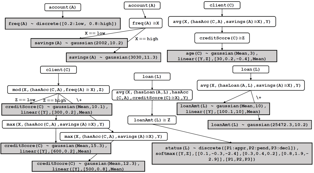
Figure 1: A collection of DLTs corresponding to the JMP in Example 5.1.

Rather than learning distributional clauses directly, we will learn distributional logic trees (DLTs), a kind of first-order decision trees (Blockeel and De Raedt, 1998) for distributional clauses. The reasons are 1) that decision trees are very effective from a machine learning perspective, and 2) that they automatically result in distributional clauses that are mutually exclusive, that is, they guarantee that the first validity requirement for DC is satisfied. This requirement states that only one distribution can be defined for each random variable in a possible world.

Formally, a DLT for an attribute, $a(T)$, is a rooted tree, where the root is an entity atom $e(T)$, each leaf is labeled by a probability distribution $\mathcal{D}_{\phi}$ and/or a statistical model $\mathcal{M}_{\psi}$, and each internal node is labeled with an atom $b_{i}$. Internal nodes $b_{i}$ can be of two types:

• a binary atom of the form $a_{j}(T)\cong V$ that unifies the outcome of an attribute $a_{j}(T)$ with a variable $V$.

• an aggregation atom of the form $aggr(X,Q,V)$, as discussed in section 4.2, where $Q$ is of the form $(r(T,T_{1}),a_{j}(T_{1})\cong X)$ in which $r$ is a link relation that relates entities of type $T$ to entities of type $T_{1}$ and $a_{j}(T_{1})$ is an attribute.

As common in decision trees, the nodes’ children are defined based on the values that the node can take; here, this corresponds to the values that $V$ can take. There are two cases to consider:

• $V$ takes discrete values $\{v_{1},...,v_{n}\}$. Then there is one child for each value $v_{i}$.

• $V$ takes numeric values. Then its value is used to estimate the parameters of the distribution $\mathcal{D}_{\phi}$ and/or the statistical model $\mathcal{M}_{\psi}$ in the leaves.

Furthermore, given that both the binary and the aggregation atom $b_{i}$ can fail, there is also an optional extra child that captures that $b_{i}$ fails and $V$ is undefined. This is reminiscent of logical decision trees, where every internal node contains a query, and there is both a success and a fail branch (Blockeel and De Raedt, 1998). Finally, the tree’s leaf nodes contain the head of the distributional clause, which is of the form $h\sim\mathcal{D}_{\phi}$. The leaf node also includes the statistical model $\mathcal{M}_{\psi}$ present in the body of the distributional clause.

Depending on the type of the random variable defined by $h$, the distribution $\mathcal{D}_{\phi}$ and the model $\mathcal{M}_{\psi}$ can be one of the three types defined in Table 2 in our current implementation of DiceML. Examples of DLTs are shown in Figure 1. It should be clear that if no continuous variable appears in the branch, then $\mathcal{M}_{\psi}$ is absent, and $\mathcal{D}_{\phi}$ is a Gaussian distribution or discrete distribution depending on the type of random variable defined by $h$.

It is straightforward to convert the DLT to a set of distributional clauses. Basically, every path from the root to a leaf node in the DLT corresponds to a distributional clause of the form $h\sim\mathcal{D}_{\phi}\leftarrow b_{1},...,b_{n},\mathcal{M}_{\psi}$.

Example 6.1.

The example of DLTs are shown in Figure 1. There is one tree for each attribute, and together these DLTs make up the JMP of Example 5.1. Consider for instance the bottom-left DLT in the collection of DLTs shown in Figure 1. The leftmost path from the root proceeding to the leaf node in the DLT corresponds to the following clause:

⬇

creditScore(C) $\sim\$ gaussian(Mean,10.1) $\leftarrow\$ client(C), mod(X,(hasAcc(C,A), freq(A)$\cong$X),low), linear([Y],[300,0.2],Mean).

We can now summarize the learning task that is tackled by DiceML as that of learning a DLT for a particular attribute. More formally,

Given:

• an attribute $a$

• training data consisting of,

  • a set of facts $\mathcal{A}_{\mathcal{DB}}\cup\mathcal{R}_{\mathcal{DB}}$ representing a relational data $\mathcal{DB}$;

  • a set of distributional clause (possibly empty) representing the background knowledge $\mathcal{BK}$;

• a declarative bias ${\cal L}$ that defines the set of distributional clauses that are allowed in hypotheses;

• a scoring function

Find: A distributional logic tree for $a$, which satisfies ${\cal L}$ and which scores best on the scoring function

Once DLTs are learned for all attributes, they are converted to clauses that together with the set of facts $\mathcal{R}_{\mathcal{DB}}$ constitute the final learned JMP.

We now describe our approach DiceML that learns JMPs. We do this in two different steps. We first present an algorithm to learn a DLT for a single attribute. Afterwards, we show how to learn a set of DLTs, that is, a JMP in an iterative EM-like manner, which is useful to deal with missing values.

6.1 Learning a Distributional Logic Tree

The distributional logic tree learner follows the standard decision tree learning algorithm sketched in Algorithm 1.

procedure induce-DLT($\mathcal{T}:tree,\leavevmode\nobreak\ \mathcal{Q}:query,\leavevmode\nobreak\ \mathcal{E}:examples$, ${\cal V}:numeric\leavevmode\nobreak\ variables$)

if $\mathcal{E}$ is not empty and sufficiently homogeneous then

compute the best clause $a(T)\sim{\cal D}_{\phi}\leftarrow Q,{\cal M}_{\psi}$ using ${\cal V}$ according to $score$

turn ${\cal T}$ into the leaf representing this clause

else

for all queries $(Q,l(V))\in\rho(Q)$ do

compute $score((Q,l(V)),\leavevmode\nobreak\ {\cal E})$

end for

let $(Q,l(V))$ be the best refinement with regard to the $score$

${\cal T}.test$ := $l(V)$

if $V$ takes discrete values $\{v_{1},...,v_{n}\}$ then

for all $v_{i}$

${\cal E}_{i}$ := the set of examples in ${\cal E}$ for which $Q,l(V),V==v_{i}$ succeeds

call induce-DLT(${\cal T}.child(i),\leavevmode\nobreak\ {\cal E}_{i},\leavevmode\nobreak\ (Q,l(V),V==v_{i}),\leavevmode\nobreak\ {\cal V})$

end for

else  %$V$ takes continuous values

${\cal E}_{v}$ := the set of examples in ${\cal E}$ for which $Q,l(V)$ succeeds

call induce-DLT(${\cal T}.child(success),\leavevmode\nobreak\ {\cal E}_{v},\leavevmode\nobreak\ (Q,l(V)),\leavevmode\nobreak\ {\cal V}\cup\{V\})$

${\cal E}_{fail}$ := the set of examples in ${\cal E}$ for which $Q,l(V)$ fails

call induce-DLT(${\cal T}.child(fail),\leavevmode\nobreak\ {\cal E}_{fail},\leavevmode\nobreak\ (Q,\backslash\mbox{+}\leavevmode\nobreak\ l(V)),\leavevmode\nobreak\ {\cal V})$

Algorithm 1 Induction of distributional logic trees

The induction process for the tree for a target attribute predicate $a(T)$ starts with the tree, and the query initialized to an entity predicate $e(T)$ of the same type as the attribute predicate, the full set of examples ${\cal E}$ and the empty set of variables ${\cal V}$. The algorithm recursively adds nodes in the tree. Before adding a node, it first tests whether the non-empty example set ${\cal E}$ is sufficiently homogeneous. If it is, it will compute the best statistical model ${\cal M}_{\psi}$ and the distribution ${\cal D}_{\phi}$ to be used in that leaf. The set ${\cal E}$ is judged sufficiently homogeneous in a tree if none of the possible splitting or refinement operations increases the score by at least $\epsilon$. Furthermore, as there is no information in an empty set of examples, the algorithm does not learn distributional clauses for branches of the tree that contain no examples.

In case the nodes should be further expanded, the standard recursive splitting procedure is followed, i.e., all possible tests $l$ to be put in the node are computed using a refinement operator $\rho$ and evaluated, the best refinement is selected and put in the node as a test, afterwards the children of the node are computed, and the procedure is called recursively. If the literal $l(V)$ produces discrete values, there is one branch per possible value; if it is continuous, there is one branch in which the value of the continuous variable $V$ will be remembered so that it can be used in the statistical model. The final branch is a fail branch corresponding to the case where the query $Q,l(V)$ fails. Such failing branches are also used in the logical decision tree learner TILDE (Blockeel and De Raedt, 1998). The process terminates when there are no attributes left to test on, or when examples at each leaf nodes are sufficiently homogeneous.

Several aspects of the algorithm still need to be explained in detail.

The refinement operator

For generating refinements of the node, the algorithm employs a refinement operator (Džeroski, 2009) that specializes the body $\mathcal{Q}$ (the conjunction of atoms in the path from the root to the node) by adding a literal $l$ to the body yielding $(\mathcal{Q},l)$, where $l$ is either a binary atom of the form $a_{j}(T)$ or an aggregation atom as discussed in the beginning of this section. The operator ensures that only the refinements that are declarative bias conform are generated. The details of the declarative bias are provided in A.

Estimating the parameters of the statistical model.

The addition of the leaf node requires one to estimate parameters of the statistical model $\mathcal{M}_{\psi}$ and/or parameters of the distribution $\mathcal{D}_{\phi}$. Let us look at the following example to understand the estimation of the parameters.

Example 6.2.

Suppose that the training data consists of the following set of facts and distributional clauses:

⬇

account(a_1). account(a_2).

freq(a_1) $\sim\$ discrete([0.2:low,0.8:high]).

freq(a_2) $\sim\$ val(low).

savings(a_1) $\sim\$ val(3000).

savings(a_2) $\sim\$ val(4000).

deposit(A) $\sim\$ gaussian(30000, 100.1) $\leftarrow\$ account(A), freq(A)$\cong$low.

deposit(A) $\sim\$ gaussian(40000, 200.2) $\leftarrow\$ account(A), freq(A)$\cong$high.

Further, suppose that a path from the root to leaf node while inducing DLT for savings corresponds to the following clause,

⬇

savings(A) $\sim\$ gaussian($\mu$,$\sigma$) $\leftarrow\$ account(A), freq(A)$\cong$low, deposit(A)$\cong$X, linear([X],[$w_{1}$,$w_{0}$],$\mu$).

where $\{w_{0},w_{1},\mu,\sigma\}$ are the parameters that we want to estimate.

There are two substitutions of the variable A, i.e., $\theta_{1}=\{\texttt{A/a\_1}\}$ and $\theta_{2}=\{\texttt{A/a\_2}\}$, that are possible for the clause. The parameters of the clause can be approximately estimated from samples of the partial possible world obtained by proving the query $\textrm{?- }h\theta_{1},\mathcal{Q}\theta_{1}$ and the samples obtained by proving the query $\textrm{?- }h\theta_{2},\mathcal{Q}\theta_{2}$. Following Equation 2, the weight $w_{{\theta}_{i}}^{(j)}$ of an $j^{th}$ sample obtained by proving a query $\textrm{?- }h\theta_{i},\mathcal{Q}\theta_{i}$ is given by,

$$w_{\theta_{i}}^{(j)}=\frac{w_{q}^{(j)}w_{e}^{(j)}}{\sum_{j=1}^{N}w_{e}^{(j)}}$$ (3)

where $w_{q}^{(j)}$ is $1$ if the $j^{th}$ sample of the partial possible world entails the query; otherwise, it is $0$. Since the evidence set is empty, $w_{e}^{(j)}$ is always $1$ here.

Suppose, we obtained the following partial possible worlds, where each world is weighted by the weight obtained using Equation 3.

⬇

[savings(a_1)$\cong$3000,account(a_1),freq(a_1)$\cong$low,deposit(a_1)$\cong$30010.1],

${w}_{\theta_{1}}^{(1)}=0.5$.

[savings(a_1)$\cong$3000,account(a_1),freq(a_1)$\cong$high,deposit(a_1)$\cong$40410.3],

${w}_{\theta_{1}}^{(2)}=0$.

[savings(a_2)$\cong$4000,account(a_2),freq(a_2)$\cong$low,deposit(a_2)$\cong$30211.3],

${w}_{\theta_{2}}^{(1)}=0.5$.

[savings(a_2)$\cong$4000,account(a_2),freq(a_2)$\cong$low,deposit(a_2)$\cong$30410.5],

${w}_{\theta_{2}}^{(2)}=0.5$.

Thus, we have four data-points (i.e., partial possible worlds) to estimate parameters. The natural way for estimating the parameters is via log-likelihood maximization. However, in our case, each data-point is weighted. In such a case, Conniffe (1987) argues that the estimation logically proceeds via expected log-likelihood maximization. So, to estimate the parameters, we maximize the expected log-likelihood of savings, that is given by the expression,

$$\begin{split}\ln(\mathcal{N}(3000\mid 30010.1w_{1}+w_{0},\sigma))\times 0.5+\ln(\mathcal{N}(3000\mid 40410.3w_{1}+w_{0},\sigma))\times 0+\\ \ln(\mathcal{N}(4000\mid 30211.3w_{1}+w_{0},\sigma))\times 0.5+\ln(\mathcal{N}(4000\mid 30410.5w_{1}+w_{0},\sigma))\times 0.5\end{split}$$ (4)

It should be clear that the same approach can be used to estimate the parameters from any distributional clauses and/or facts present in the training data.

Notice from the above example that substitutions of the clause are required to estimate the clause’s parameters. We call such substitutions examples and define them formally,

Definition 6.1.

(Examples at the leaf node) Given the training data and a path from the root to a leaf node $L$ corresponding to a clause $h\sim\mathcal{D}_{\phi}\leftarrow\mathcal{Q},\mathcal{M}_{\psi}$, we define the examples ${\cal E}$ at the leaf node $L$ to be the set of substitutions of the clause that ground all entity relations, link relations and attributes in the clause.

Generalizing from Equation 4, parameters of any distribution and/or of any statistical model at any leaf node can be estimated by maximizing the expected log-likelihood $E(\boldsymbol{\varphi})$, which is given by the following expression,

$$E(\boldsymbol{\varphi})=\sum_{\theta_{i}\in\mathcal{E}}\sum_{j=1}^{N}\ln(p(h\theta_{i}\mid\boldsymbol{\varphi},{\cal V}\theta_{i}^{(j)})){w}_{\theta_{i}}^{(j)}$$ (5)

where $\boldsymbol{\varphi}$ is the set of parameters, ${\cal E}$ is the set of examples at the leaf node, ${\cal V}$ is the set of continuous variables in $\mathcal{Q}$, $N$ is the number of times the query $\textrm{?- }h\theta_{i},\mathcal{Q}\theta_{i}$ is proved, ${w}_{\theta_{i}}^{(j)}$ is the weight of the $j^{th}$ sample, ${\cal V}\theta_{i}^{(j)}$ is $j^{th}$ sample of continuous random variables and $p(h\theta_{i}\mid\boldsymbol{\varphi},{\cal V}\theta_{i}^{(j)})$ is the probability distribution of the random variable $h\theta_{i}$ given $\boldsymbol{\varphi}$ and ${\cal V}\theta_{i}^{(j)}$. For the three simpler statistical models that we considered, the expected log-likelihood is a convex function. DiceML uses scikit-learn (Pedregosa et al., 2011) to obtain the maximum likelihood estimate $\widehat{\boldsymbol{\varphi}}$ of the parameters.

The Scoring Function

Clauses are scored using the Bayesian Information Criterion (BIC, Schwarz, 1978) for selecting the best among the set of candidate clauses. The score of a clause $h\sim\mathcal{D}_{\phi}\leftarrow\mathcal{Q},\mathcal{M}_{\psi}$, which corresponds to a path from the root to a leaf, is given by,

$$s(h\sim\mathcal{D}_{\phi}\leftarrow\mathcal{Q},\mathcal{M}_{\psi})=2E(\widehat{\boldsymbol{\varphi}})-k\ln|{\cal E}|$$ (6)

where $|{\cal E}|$ is the number of examples ${\cal E}$ at the leaf, $k$ is the number of parameters. The score avoids over-fitting and naturally takes care of the different number of examples at different leaves. To determine the score of the refinement $(\mathcal{Q},l(V))$ of the clause, where $V$ takes discrete values $\{v_{1},\dots,v_{n}\}$, the score of $n+1$ clauses corresponding to $n+1$ branches are summed. That is, the score of the refinement is given by,

$$score((\mathcal{Q},l(V)),\mathcal{E}_{V})=s(h\sim\mathcal{D}_{\phi_{1}}\leftarrow\mathcal{Q},l(V),V==v_{1},\mathcal{M}_{\psi_{1}})+\dots+$$ (7)

$$s(h\sim\mathcal{D}_{\phi_{n}}\leftarrow\mathcal{Q},l(V),V==v_{n},\mathcal{M}_{\psi_{n}})+s(h\sim\mathcal{D}_{\phi_{fail}}\leftarrow\mathcal{Q},\backslash\mbox{+}\ l(V),\mathcal{M}_{\psi_{fail}})$$

where ${\cal E}_{V}$ is the number of substitutions to the clause $h\sim\mathcal{D}_{\phi_{V}}\leftarrow\mathcal{Q},l(V),\mathcal{M}_{\psi_{V}}$. The score is computed in the similar manner when $V$ takes continuous value.

Learning Joint Model Programs

To learn our final joint model program $\mathbb{P}_{\mathcal{DB}}$, we induce DLTs, in an order defined by the user in the declarative bias, separately for each attribute predicate. Recall that valid DC programs require the existence of a rank assignment $\prec$ over predicates of the program. The order declares the rank assignment over attributes. Each path from the root to the leaf node in each DLT corresponds to a clause in the program $\mathbb{P}_{\mathcal{DB}}$. This program defines the joint probability distribution and probabilistic inference in this program can be used to compute a probability distribution over any set of cells given the observed value of any other set of cells.

6.2 Learning JMPs in the Presence of Missing Data

We explore two approaches in this paper:

6.2.1 Handling missing data using negated literals

One approach of learning probabilistic models from missing data that we have emphasized so far is to treat missing values as a separate category and learn conditional distributions also for this category. By reserving one branch in the internal nodes for missing values (negation), DLTs do specify distributions for the target attribute ($a$) in the condition when values are missing. This branch corresponds to the negated literal in the distributional clause.

Example 6.3.

Consider DLT for loanAmt (“loan amount”) in the collection of DLTs shown in Figure 1. The rightmost path from the root proceeding to the leaf node in the DLT corresponds to the clause with negated literal:

⬇

loanAmt(L) $\sim\$ gaussian(25472.3,10.2) $\leftarrow\$ loan(L), \+avg(X, (hasLoan(A,L), savings(A)$\cong$X), Y).

The above clause specifies a distribution from which the loan amount is drawn if the loan has no account or the loan has accounts but the savings of these accounts are missing.

There are other approaches of learning probabilistic models from missing data. The most common approach is Expectation-Maximization (EM). We discuss this approach next.

6.2.2 Learning JMPs using the stochastic EM

In this approach, we learn programs iteratively by explicitly modeling the missing data and start with the program learned so far. To realize this, we learn programs inside the stochastic EM algorithm (Diebolt and Ip, 1995). In this setting, we assume that background knowledge is not present.

Consider a training multi-relational tables $\mathcal{DB}$ with missing cells $\mathbf{Z}=\{Z_{1},\dots,Z_{m}\}$ and observed cells $\{X_{1}\cong x_{1},\dots,X_{n}\cong x_{n}\}$ (abbreviated as $\mathbf{X}\cong\mathbf{x}$), where $x_{i}$ is the value of the observed cell $X_{i}$. The iterative procedure starts by first learning a program $\mathbb{P}_{\mathcal{DB}}^{0}$ with negated literals from data with missing cells — using the same algorithm (Algorithm 1), subsequent programs are learned from data after filling missing cells with their sampled joint state. Formally, given the current learned program $\mathbb{P}_{\mathcal{DB}}^{i}$ specifying a probability distribution $p(\mathbf{X},\mathbf{Z})$, the ($i+1$)-th EM step is conducted in two steps:

E-step

A sample $\{Z_{1}\cong z_{1},\dots,Z_{m}\cong z_{m}\}$ (abbreviated as $\mathbf{Z}\cong\mathbf{z}$) of the missing cells $\mathbf{Z}$ is taken from the conditional probability distribution $p(\mathbf{Z}\mid\mathbf{X\cong x})$. The missing cells $\mathbf{Z}$ are filled in the tables by asserting the facts $\{Z_{1}\sim val(z_{1}),\dots,Z_{m}\sim val(z_{m})\}$ (abbreviated as $\mathbf{Z}\sim val(\mathbf{z})$) in the training data.

M-step

A new program ${\mathbb{P}_{\mathcal{DB}}^{i+1}}$ is learned from the training data , and subsequently facts $\mathbf{Z}\sim val(\mathbf{z})$ are retracted from the training data. However, in this case, the parameters of distribution and/or statistical models at the leaf node are estimated by maximizing the log-likelihood rather than maximizing the expected log-likelihood. This is because, in this case, the training data does not consist of probabilistic facts or distributional clauses. Following equation 5, the log-likelihood function $L(\boldsymbol{\varphi})$ is given by the following expression,

$$L(\boldsymbol{\varphi})=\sum_{\theta_{i}\in\mathcal{E}}\ln(p(h\theta_{i}\mid\boldsymbol{\varphi},{\cal V}\theta_{i}^{(j)}))$$ (8)

The number of iterations decides the termination of the procedure. It is worth noting that we learn the structure as well as the parameters of the program $\mathbb{P}_{\mathcal{DB}}$, which is more challenging compared to learning only parameters of the model as in the case of standard stochastic EM. In the experiment, we demonstrate that the program learned at the end of stochastic EM procedure performs better compared to the learned program using the previous approach (Section 6.2.1).

The learning algorithm presented in this section is similar to the standard structural EM algorithm for learning Bayesian networks (Friedman, 1997). The main difference, apart from having different target representations (DC vs. Bayesian networks), is that structural EM uses the standard EM (Dempster et al., 1977) for structure learning. Our approach uses the stochastic EM for structure learning for the tractability reasons (hybrid probabilistic inference in large relational data is computationally very challenging).

7 Experiments

This section empirically evaluates JMPs learned by DiceML. We first describe the data sets that we used, and then explain the research questions that we address.

We used the same data sets as used in Ravkic et al. (2015) to evaluate a hybrid relational model. Details of these data sets are as follows:

Synthetic University Data Set

This data set contains information of $800$ students, $125$ courses and $125$ professors with three attributes in the data set being continuous while the rest three attributes being discrete. For example, the attribute intelligence/1 represents the intelligence level of students in the range $[50.0,180.0]$ and the attribute difficulty/1 represents the difficulty level of courses that takes three discrete values $\{easy,med,hard\}$. The data set also contains three relations: takes/2, denoting which course is taken by a student; friend/2, denoting whether two students are friends and teaches/2, denoting which course is taught by a professor.

Real-world PKDD’99 Financial Data Set

This data set is generated by processing the financial data set from the PKDD’99 Discovery Challenge. The data set is about services that a bank offers to its clients, such as loans, accounts, and credit cards. It contains information of four types of entities: $5,358$ clients, $4,490$ accounts, $680$ loans and $77$ districts. Ten attributes are of the continuous type, and three are of the discrete type. The data set contains four relations: hasAccount/2 that links clients to accounts; hasLoan/2 that links accounts to loans; clientDistrict/2 that links clients to districts; and finally clientLoan/2 that links clients to loans. This data set is split into ten folds considering account to be the central entity. All information about clients, loans, and districts related to one account appear in the same fold.

In addition to these benchmark data sets, we also performed experiments with one more data set:

Real-world NBA Data Set

This data set is about basketball matches from the National Basketball Association (Schulte and Routley, 2014). It records information about matches played between two teams and actions performed by each player of those two teams. There are $30$ teams, $30$ games, $392$ players and $767$ actions. In total, there are $19$ attributes, and all of them are of integer type. We treated $18$ as continuous and $1$ attribute, i.e., resultofteam1/1 that takes two values $\{win,loss\}$ as discrete. This data set also contains relations, such as, team1id/2 that specifies the first team of matches, team2id/2 that specifies the second team of matches, teamid/3 that relates matches, players and teams. Considering the match to be a central entity, $90\%$ of the data set was used for training and the rest for testing.

Specifically, we address the following questions:

Question 7.1.

How does the performance of JMPs learned by DiceML compare with the state-of-the-art hybrid relational models when trained on a fully observed data?

We compared JMPs learned by DiceML, in the case of fully observed data, with the model learned by the state-of-the-art algorithm Learner of Local Models - Hybrid (LLM-H) introduced by Ravkic et al. (2015). The LLM-H algorithm learns a joint probabilistic relational model in the form of a hybrid relational dependency network (HRDN). This algorithm requires training data to be fully observed. To evaluate HRDNs, (Ravkic et al., 2015) followed the methodology of predicting an attribute of an instance in the testing data, using the rest of the testing data as observed. We followed the same methodology in this experimental setting. In addition to HRDNs, we also compared the performance of JMPs with individual DLTs learned for each attribute separately. Indeed on fully observed data, we could learn individual DLTs and use just one DLT to predict an attribute. However, then we could not deal with the autocompletion task, i.e., predicting any set of cells given any other set of cells. The current experimental setting, i.e., predicting a cell given all other cells, is simple compared to the autocompletion setting (our original problem). For clarity, we summarize the differences between these three models in Table 3.

Individual DLTs	HRDNs	JMPs
Individual models trained for individual attributes	Joint models specifying a joint probability distribution over all attributes	Joint models specifying a joint probability distribution over all attributes
Can make use of negated literals to deal with missing data	Can not deal with missing data	Can be trained using EM to deal with missing data and can also make use of negated literals
Can not be used for the autocompletion task that requires probabilistic inference	Can not be used for the autocompletion task	Can be used for the autocompletion task

Table 3: Differences between individual DLTs, HRDNs, and JMPs.

Nonetheless, we performed this experiment as a sanity check to ensure that i) the individual DLTs that we learn are not worse than HRDNs and ii) the JMPs are not significantly worse than those DLTs. Even though we do not expect JMPs to be generally better since learning joint models has no advantage over learning individual models when training data is fully observed. Joint models can infer using both predictive and diagnostic information (Pearl, 1988), while individual models can only use predictive information.

We used the same evaluation metrics as used in Ravkic et al. (2015) to evaluate the quality of predictions of JMPs.

Evaluation metric

To measure the predictive performance for discrete attributes, multi-class area under ROC curve ($\textrm{AUC}_{\textrm{total}}$) (Provost and Domingos, 2000) was used, whereas normalized root-mean-square error (NRMSE) was used for continuous attributes. The NRMSE of an attribute ranges from 0 to 1 and is calculated by dividing the RMSE by the range of the attribute. To measure the quality of the probability estimates, weighted pseudo-log-likelihood (WPLL) (Kok and Domingos, 2005) was used, which corresponds to calculating pseudo-log-likelihood of instances of an attribute in the test data set and dividing it by the number of instances in the test data set.

Evaluation	Predicate	HRDN	JMP	DLT
$\textrm{AUC}_{\textrm{total}}$	gender/1	0.50 $\pm$ 0.01	0.52 $\pm$ 0.03	0.50 $\pm$ 0.03
	freq/1	0.82 $\pm$ 0.01	0.77 $\pm$ 0.07	0.83 $\pm$ 0.04
	loanStatus/1	0.66 $\pm$ 0.04	0.82 $\pm$ 0.05	0.79 $\pm$ 0.04
NRMSE	clientAge/2	0.28 $\pm$ 0.02	0.24 $\pm$ 0.02	0.24 $\pm$ 0.01
	avgSalary/1	0.13 $\pm$ 0.02	0.18 $\pm$ 0.01	0.24 $\pm$ 0.00
	ratUrbInhab/1	0.20 $\pm$ 0.00	0.25 $\pm$ 0.01	0.18 $\pm$ 0.00
	avgSumOfW/1	0.02 $\pm$ 0.00	0.02 $\pm$ 0.00	0.03 $\pm$ 0.01
	avgSumOfCred/1	0.02 $\pm$ 0.00	0.02 $\pm$ 0.01	0.03 $\pm$ 0.01
	stdOfW/1	0.05 $\pm$ 0.01	0.05 $\pm$ 0.01	0.05 $\pm$ 0.00
	stdOfCred/1	0.05 $\pm$ 0.01	0.04 $\pm$ 0.00	0.04 $\pm$ 0.00
	avgNrWith/1	0.15 $\pm$ 0.01	0.11 $\pm$ 0.00	0.11 $\pm$ 0.01
	loanAmount/1	0.16 $\pm$ 0.02	0.12 $\pm$ 0.01	0.11 $\pm$ 0.01
	monthlyPayments/1	0.18 $\pm$ 0.02	0.14 $\pm$ 0.01	0.15 $\pm$ 0.02

Table 4: The performance of JMP compared to HRDN and single trees for each attribute (DLT) on fully observed PKDD’99 financial data set. The best results (mean $\pm$ standard deviation) are in bold.

Predicate	HRDN	JMP	DLT
nrhours/1	-4.48	-3.39	-3.20
difficulty/1	-0.02	-0.00	-0.03
ability/1	-5.34	-3.83	-3.77
intelligence/1	-4.66	-4.08	-3.37
grade/2	-1.45	-1.00	-1.00
satisfaction/2	-1.54	-1.05	-1.05
Total WPLL	-17.49	-13.35	-12.42

Table 5: WPLL for each attribute on fully observed university data set, consisting of 800 students, 125 courses, and 125 professors. The best results are in bold.

Predicate	HRDN	JMP	DLT
plusminus/2	-5.38	-3.68	-3.62
defensiverebounds/2	-3.56	-2.14	-2.12
fieldgoalsmade/2	-1.66	-0.58	-1.03
assists/2	-3.10	-1.93	-1.91
blocksagainst/2	-1.36	-0.84	-0.76
freethrowsmade/2	-1.52	-1.25	-1.16
offensiverebounds/2	-2.27	-1.36	-1.41
threepointattempts/2	-0.00	-0.00	-0.00
threepointsmade/2	-0.00	-0.00	-0.00
starter/2	-0.67	-0.70	-0.36
turnovers/2	-2.45	-1.56	-1.55
personalfouls/2	-2.44	-1.67	-1.60
freethrowattempts/2	-1.66	-0.98	-0.99
points/2	-2.87	-1.84	-1.90
minutes/2	-10.91	-7.21	-7.21
steals/2	-1.63	-1.03	-1.03
fieldgoalattempts/2	-3.30	-1.98	-1.98
blockedshots/2	-1.37	-0.81	-0.81
resultofteam1/1	-2.05	-0.00	-0.00
Total WPLL	-48.22	-29.56	-29.45

Table 6: WPLL for each attribute on the NBA data set. The best results are in bold.

In our experiment, we used the aggregation function average for continuous attributes, and mode and cardinality for discrete attributes. An ordering chosen randomly among attributes was provided in the declarative bias. While training individual DLTs, ordering among attributes was not considered since those DLTs were not joint models but individual models for each attribute. We used the same data with the same settings as in Ravkic et al. (2015) to compare the performance of our algorithm. Table 4 shows the comparison on financial data set using 10-fold cross-validation. During testing, prediction of a test cell was the mode of the probability distribution of the cell obtained by conditioning over the rest of the test data. A Bayes-ball algorithm (Shachter, 1998) that performs lazy grounding of the learned program was used to find the evidence that was relevant to the test cell. Table 5 shows the comparison on university data set divided into training and testing set. Numbers for HRDNs on these two data sets are taken directly from Ravkic et al. (2015). Table 6 shows the result on the additional data set, i.e., the NBA data set.

We observe that on several occasions, JMPs outperforms HRDNs, although both of these approaches use the same features to learn classification and regression models for attributes. This observation can be explained by the fact that LLM-H learns tabular conditional probability distributions (CPDs) while DiceML learns tree-structured CPDs with much fewer parameters. (Chickering et al., 1997; Friedman and Goldszmidt, 1998; Breese et al., 1998) observed that tree-structured CPDs are a more efficient way of automatically learning propositional probabilistic models from data. Unsurprisingly, we observe similar behavior for relational models as well. Apart from better performance, tree-structured CPDs make JMPs more interpretable. JMPs are human-readable programs while HRDNs are not. As already discussed, we expect that single models for attributes, i.e., individual DLTs outperform both joint models, i.e., JMPs and HRDNs. It is worth reiterating that individual models can not be used for the autocompletion task, while joint models can be used.

The experiment suggests that JMPs learned by DiceML can outperform the state-of-the-art algorithm for fully observed data.

Question 7.2.

Can DiceML utilize background knowledge while learning distributional clauses?

Background knowledge provides additional information about attributes that can be probabilistic when expressed as the set of distributional clauses. A learning algorithm that can utilize this information along with the training data can learn a better model. We performed this experiment to examine whether DiceML can also learn a DLT for a single attribute (a set of clauses for an attribute) from the training data along with background knowledge expressed as a set of distributional clauses. This learning task is a more complex task than the previous task, where we learned individual DLTs from only training data, since this task involves probabilistic inference along with learning.

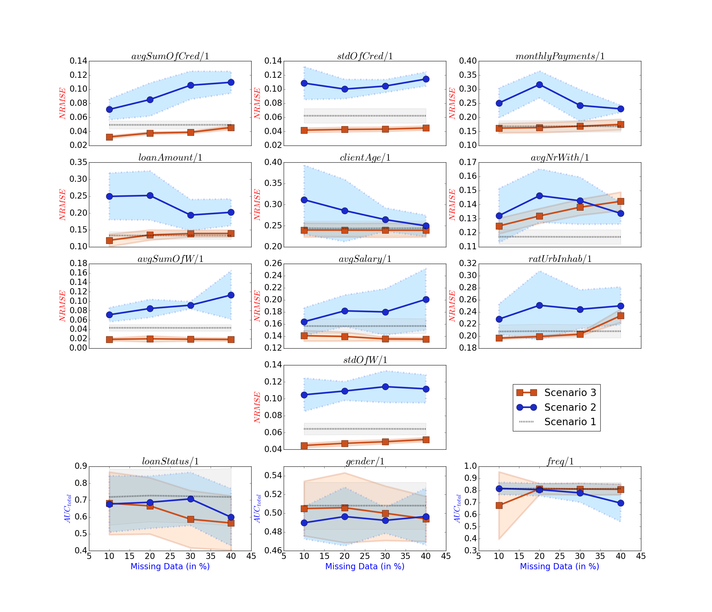
Figure 2: Performance of models learned in the three scenarios (Question 7.2) versus the percentage of removed cells. The bottom three figures show $\textrm{AUC}_{\textrm{total}}$ of discrete attributes, whereas, the upper ten figures show NRMSE of continuous attributes. Less NRMSE is better while more $\textrm{AUC}_{\textrm{total}}$ is better.

We used the financial data set divided into ten folds. Two folds ($T$) were used for training the DLT for an attribute; one fold was used for testing that DLT; and seven folds were used for generating background knowledge $BK$, which was a set of distributional clauses for all attributes, i.e., a JMP. We considered three scenarios: 1) A DLT for an attribute was induced from the training set $T$; subsequently, the DLT was used to predict the attribute in the test fold. 2) A partial data set $T^{\prime}$ was generated by removing $x\%$ of cells at random from the training set $T$. Subsequently, a DLT for the same attribute was induced from the partial set $T^{\prime}$. Note that the DLT can be induced from partial data since we allow negated literals in the body of clauses. 3) A DLT for the same attribute was induced from the partial set $T^{\prime}$ as well as $BK$.

The predictive performance in the test set for the three scenarios, varying the percentage of removed cells, is shown in Figure 2. Compared to the second scenario, much lower NRMSE is observed in the third scenario. On several occasions, DLTs learned in the third scenario, even outperform the same learned in the first scenario. Note that $BK$ is itself a probabilistic model learned from seven folds of data and is rich in knowledge.

These results lead to the conclusion that DiceML can learn distributional clauses from the training data utilizing additional probabilistic information from background knowledge.

Question 7.3.

Can DiceML learn JMPs from relational data when a large portion of the data is missing?

Probabilistic inference in a hybrid relational joint model is challenging. An even more challenging task, which requires numerous such inferences, is learning such models from partially observed relational data. We evaluated the performance of JMPs learned by DiceML from such data. To the best of our knowledge, no system in the literature can learn such models from the partially observed relational data with continuous as well as discrete attributes. We used the financial data set and performed the following experiment to answer the question.

We randomly removed some percentage of cells from the client, loan, account, and district tables of the financial data set to obtain a partial data set. Then we trained three models to predict attributes in the test data set. The first model was a JMP obtained by performing stochastic EM on the partial data set. The second model was just an individual model, i.e., a DLT for each attribute trained on the partial data set. It is worth reiterating that the DLT can be learned even when some cells are missing since we allow negated literals in the body of distributional clauses. The last model was also an individual DLT for each attribute but was trained on the complete training data set. The performance of these models is shown in Figure 3. Nine folds of the data set were used for training, and the rest for testing. The variance of NRMSE/$\textrm{AUC}_{\textrm{total}}$ is shown by shaded region when the experiment was repeated ten times on this data set. We observe that the JMP obtained using EM performs better, for most of the attributes, than individual DLTs trained on the partial data set. As expected, DLTs trained on the complete data perform best. The convergence of the stochastic EM after few iterations is shown in Figure 5. To obtain this figure, the JMP was obtained from the financial data set with $10\%$ of cells removed using EM. This figure shows the data log-likelihood after each iteration of EM compared with the data log-likelihood when the JMP was obtained from the complete data.

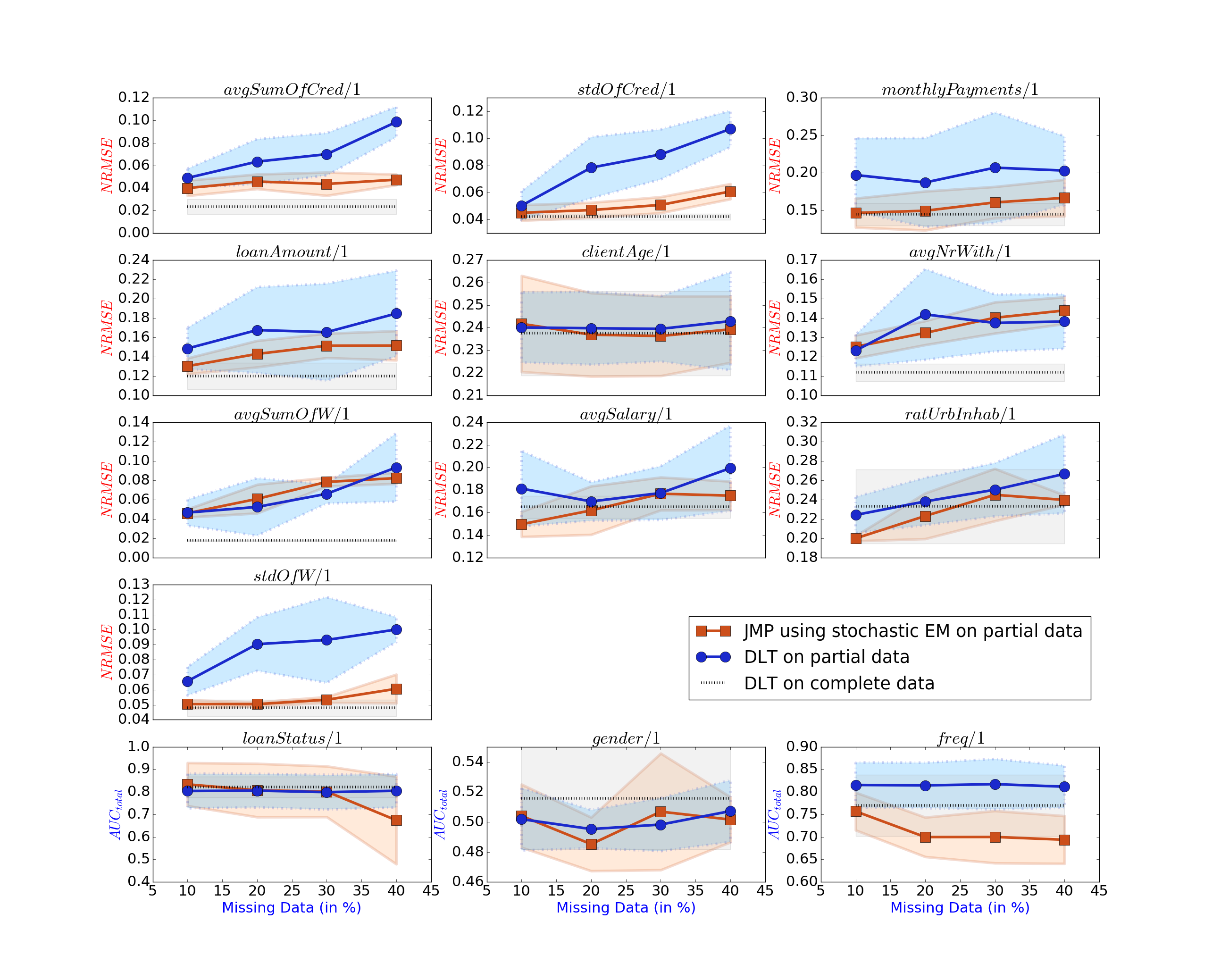
Figure 3: Performance of the three models (Question 7.3) on the financial data set versus the percentage of removed cells. The bottom three figures show $\textrm{AUC}_{\textrm{total}}$ of discrete attributes, whereas, the upper ten figures show NRMSE of continuous attributes. Less NRMSE is better while more $\textrm{AUC}_{\textrm{total}}$ is better.

The experimental environment was an Intel(R) Xeon(R) E5-2640 v3 2.60GHz CPU, 128GB RAM server running Ubuntu 18.04.4 LTS (64 bit). On the financial data set, DiceML took approximately $226$ seconds to learn the JMP in each iteration of EM. The time required to sample a joint state of missing data from this program is shown in Table 7.

Results for the same experiment on the NBA data set is shown in Figure 4. We observe that when a large portion of data is missing, the JMP learned using stochastic EM performs better than individual DLTs. When $40\%$ of data is missing, the JMP performs better on $11$ attributes out of $19$ attributes. On $3$ attributes, the performance is the same. On $5$ attributes, individual DLTs perform better.

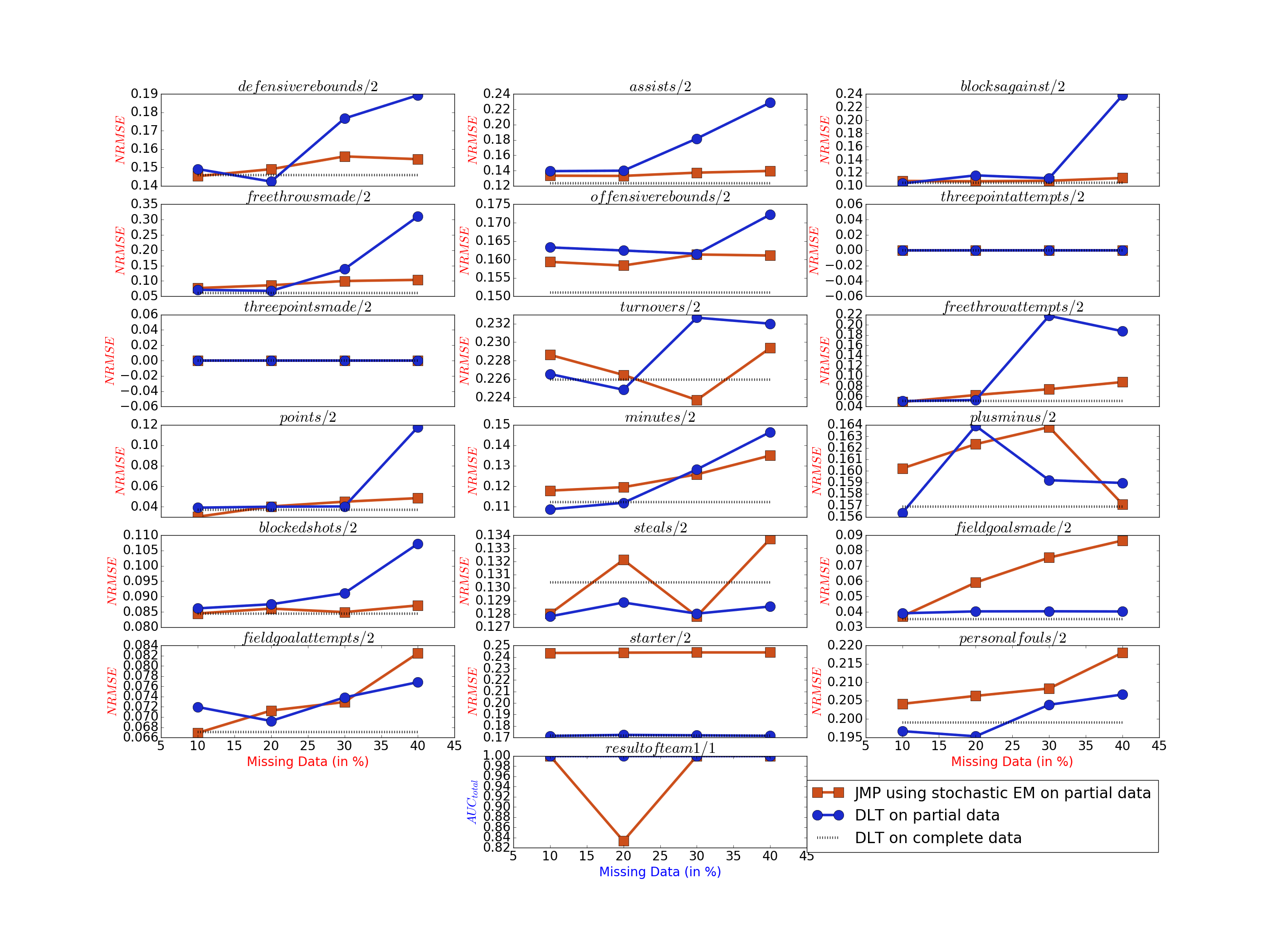
Figure 4: Performance of the three models, discussed for Question 7.3, on the NBA data set. The bottom figure show $\textrm{AUC}_{\textrm{total}}$ of the discrete attribute, whereas, the upper eighteen figures show NRMSE of continuous attributes. Less NRMSE is better while more $\textrm{AUC}_{\textrm{total}}$ is better.

All these results demonstrate that DiceML can learn JMPs even when a large portion of data is missing.

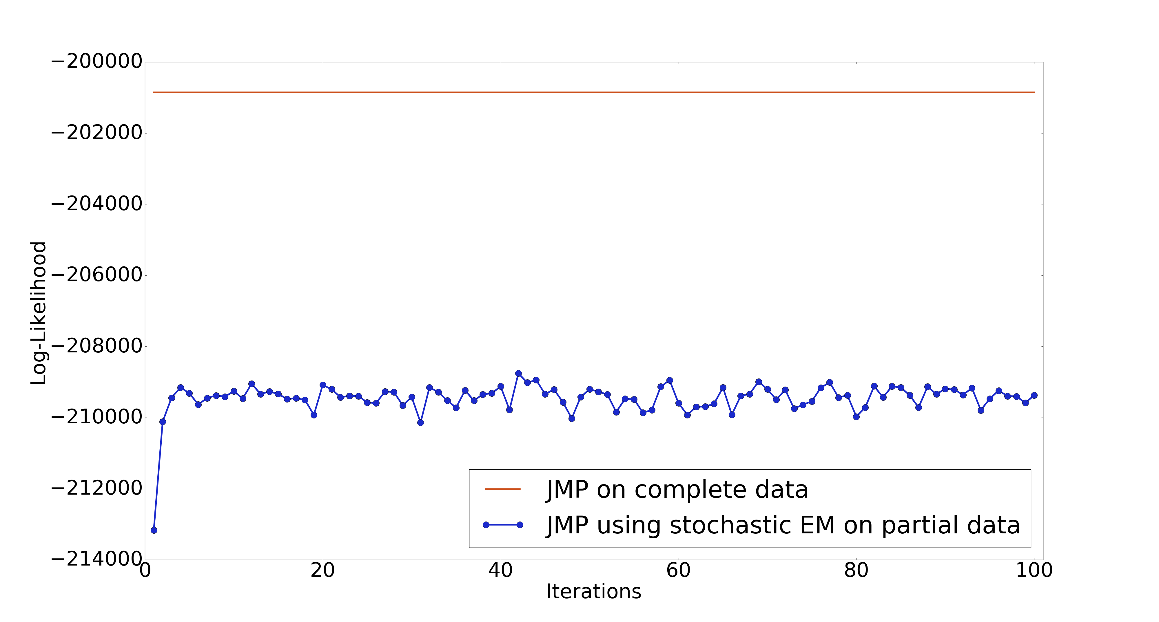
Figure 5: The convergence of the stochastic EM on the financial data set

Percentage of missing cells	number of missing cells	Time in secs (approx.)
10%	3530	131
20%	7062	113
30%	10595	97
40%	14125	72

Table 7: The time taken to draw a joint state of missing data from the joint distribution.

8 Conclusions

We presented DiceML, a probabilistic logic programming based approach for tackling the problem of autocompletion in multi-relational tables. We first integrate distributional clauses with statistical models. Then these clauses are used to represent a hybrid relational model in the form of a DC program. Such a program is capable of defining a complex probability distribution over the entire related tables. Probabilistic inference in this program allows predicting any set of cells given any other set of cells required by the autocompletion task. Since DC is expressive, we can map related tables to a set of facts in the DC language. In line with the approaches to (probabilistic) inductive logic programming, our approach learns such programs automatically from the set of facts and can make use of additional probabilistic background knowledge, if available. We demonstrated that such programs learned from fully observed relational data can outperform the state-of-the-art hybrid relational model. Another advantage of such programs over existing models is that such programs are interpretable. Although inference in hybrid relational models is hard, we demonstrated that the program learned by DiceML performs well, even when a large portion of data is missing. DiceML combines stochastic EM with structure learning to realize this.

Appendix A Declarative Bias

The use of declarative bias, which allows users to declaratively specify the search space of possible clauses to be explored while learning, is common in ILP systems such as PROGOL (Muggleton, 1995), TILDE (Blockeel and De Raedt, 1998), CLAUDIEN (De Raedt and Dehaspe, 1997), ALEPH (Srinivasan, 2001), etc. When the space is potentially huge, it plays an important role in restricting the search to finite and meaningful clauses. For our purposes, we adapt the bias declarations from (De Raedt, 2008). In DiceML, the bias consists of four types of declarations, i.e., type, mode, rand, and rank declarations. We describe them in turn with examples:

Types:

All functors are accompanied by type declarations of the form $type(func(t_{1},\cdots,t_{n}))$, where $t_{i}$ denotes the type of the $i$-th argument, i.e., the domain of the variable. For instance, consider the type declarations in Figure 6. Since the first argument of hasAcc/2 should be different type than the argument of freq/1, the clause

⬇

age(C)$\sim\$gaussian(30, 2.1) $\leftarrow\$ mod(X,(hasAcc(C,A),freq(C)$\cong$X),low).

is not type conform, but the following clause is:

⬇

age(C)$\sim\$gaussian(30, 2.1) $\leftarrow\$ mod(X,(hasAcc(C,A),freq(A)$\cong$X),low).

Modes:

We also employ modes, which is standard in ILP, for each attribute. Modes specify the form of literal $b_{i}$ in the body of the clause $h\sim\mathcal{D}_{\phi}\leftarrow b_{1},\dots,b_{n},\mathcal{M}_{\psi}$. A mode declaration is an expression of the form $mode(a_{1},aggr,(r(m_{1},\dots,m_{j}),a_{2}(m_{k})))$, where $m_{i}$ are different modes associated with variables of functors, $aggr$ is the name of aggregation function, $r$ is the link relation, and $a_{i}$ are attributes. The expression specifies the candidate aggregation functions considered while learning clauses for the attribute $a_{1}$. If the link relation is absent, then the aggregation function is not needed, so the mode declaration reduces to the form $mode(a_{1},none,a_{2}(m_{k})))$. The modes $m_{i}$ can be either input (denoted by “$+$”) or output (denoted by “$-$”). The input mode specifies that at the time of calling the functor the corresponding argument must be instantiated, the output mode specifies that the argument will be instantiated after a successful call to the functor. Consider the mode declarations in Figure 6. The clause

⬇

age(C)$\sim\$gaussian(30, 2.1) $\leftarrow\$ mod(X,(cliLoan(C,L1),status(L2)$\cong$X),appr).

is not mode conform since the first argument of cliLoan/2, i.e., the variable C does not satisfy the output mode and the variable L2 does not satisfy the input mode. The following clause, however, satisfies the mode:

⬇

age(C)$\sim\$gaussian(30, 2.1)$\leftarrow\$mod(X,(cliLoan(C1,L1),status(L1)$\cong$X),appr).

Rand Declarations:

They are used to define the type of random variables (i.e., discrete or continuous) and to specify the domain of discrete random variables.

Rank Declarations:

As we have already seen in Section 3.2, the second validity condition of the DC program requires the existence of a rank assignment $\prec$ over predicates of the program. Hence, we introduce these declarations, to specify the rank assignment over attributes. While learning distributional clauses for a single attribute, the rank declaration is not used, it is crucial while learning DC programs.

% Type declarations type(client(c)). type(loan(l)). type(account(a)). type(hasAcc(c,a)). type(hasLoan(c,l)). type(age(c)). type(creditScore(c)). type(loanAmt(l)). type(status(l)). type(savings(a)). type(freq(a)). % Mode declaration mode(age,none,creditScore(+)). mode(age,sum,(hasAcc(+,-),savings(+))). mode(age,avg,(hasAcc(+,-),savings(+))). mode(age,mod,(hasAcc(+,-),freq(+))). mode(age,max,(cliLoan(+,-),loanAmt(+))). mode(age,mod,(cliLoan(-,-),status(+))). mode(status,none,loanAmt(+)). mode(status,mod,(hasLoan(-,+),age(+))). ⋮ % Rank declaration rank([age,creditScore,loanAmt,

status,savings,freq]). % Random variable declaration rand(age,continuous,[]). rand(creditScore,continuous,[]). rand(loanAmt,continuous,[]). rand(status,discrete,[appr,pend,decl]). rand(savings,continuous,[]). rand(freq,discrete,[low,high]). % Transformed tables client(ann). loan(l_20). account(a_10). age(ann) $\sim$ val(33). creditScore(john) $\sim$ val(700). savings(a_10) $\sim$ val(3050). freq(a_10) $\sim$ val(high). loanAmt(l_20) $\sim$ val(20050). hasAcc(ann,a_11). hasLoan(a_11,l_20). ⋮ % Background knowledge age(carl) $\sim$ gaussian(40,5.1). cliLoan(C,L)$\leftarrow$hasAcc(C,A),hasLoan(A,L).

Figure 6: An example of input to DiceML, which consists of a transformation of the spreadsheet in Table 1, along with background knowledge and declarative bias.

Example A.4.

An example of the input to DiceML is shown in Figure 6, where Table 1 is converted into facts, and background knowledge is expressed using distributional clauses. The first clause in the background knowledge shown in the bottom-right of the figure states that the age of carl follows a Gaussian distribution, and the second clause states that if a client has an account in the bank and the account is linked to a loan account, then the client also has a loan.

References

- Alberti et al. (2017) Alberti, M., Bellodi, E., Cota, G., Riguzzi, F., and Zese, R. 2017. cplint on swish: Probabilistic logical inference with a web browser. Intelligenza Artificiale 11, 1, 47–64.
- Bekker and Davis (2020) Bekker, J. and Davis, J. 2020. Learning from positive and unlabeled data: a survey. Machine Learning 109, 719–760.
- Blockeel and De Raedt (1998) Blockeel, H. and De Raedt, L. 1998. Top-down induction of first-order logical decision trees. Artificial intelligence 101, 1-2, 285–297.
- Boutilier et al. (1996) Boutilier, C., Friedman, N., Goldszmidt, M., and Koller, D. 1996. Context-specific independence in bayesian networks. In Proceedings of the Twelfth international conference on Uncertainty in artificial intelligence. Morgan Kaufmann Publishers Inc., 115–123.
- Breese et al. (1998) Breese, J. S., Heckerman, D., and Kadie, C. 1998. Empirical analysis of predictive algorithms for collaborative filtering. In Proceedings of the Fourteenth conference on Uncertainty in artificial intelligence. Morgan Kaufmann Publishers Inc., 43–52.
- Chickering et al. (1997) Chickering, D. M., Heckerman, D., and Meek, C. 1997. A bayesian approach to learning bayesian networks with local structure. In Proceedings of the Thirteenth conference on Uncertainty in artificial intelligence. Morgan Kaufmann Publishers Inc., 80–89.
- Choi et al. (2010) Choi, J., Amir, E., and Hill, D. J. 2010. Lifted inference for relational continuous models. In Proceedings of the Twenty-Sixth Conference on Uncertainty in Artificial Intelligence. UAI’10. AUAI Press, Arlington, Virginia, USA, 126–134.
- Conniffe (1987) Conniffe, D. 1987. Expected maximum log likelihood estimation. Journal of the Royal Statistical Society: Series D (The Statistician) 36, 4, 317–329.
- De Raedt (2008) De Raedt, L. 2008. Logical and relational learning. Springer Science & Business Media.
- De Raedt et al. (2018) De Raedt, L., Blockeel, H., Kolb, S., Teso, S., and Verbruggen, G. 2018. Elements of an automatic data scientist. In International symposium on intelligent data analysis. Lecture Notes in Computer Science, vol. 11191. Springer, 3–14.
- De Raedt and Dehaspe (1997) De Raedt, L. and Dehaspe, L. 1997. Clausal discovery. Machine Learning 26, 2-3, 99–146.
- De Raedt et al. (2015) De Raedt, L., Dries, A., Thon, I., Van Den Broeck, G., and Verbeke, M. 2015. Inducing probabilistic relational rules from probabilistic examples. In Proceedings of the 24th International Conference on Artificial Intelligence. IJCAI’15. AAAI Press, 1835–1843.
- De Raedt et al. (2007) De Raedt, L., Kimmig, A., and Toivonen, H. 2007. Problog: A probabilistic prolog and its application in link discovery. In Proceedings of the 20th International Joint Conference on Artifical Intelligence. IJCAI’07. Morgan Kaufmann Publishers Inc., San Francisco, CA, USA, 2468–2473.
- Dempster et al. (1977) Dempster, A. P., Laird, N. M., and Rubin, D. B. 1977. Maximum likelihood from incomplete data via the em algorithm. Journal of the Royal Statistical Society: Series B (Methodological) 39, 1, 1–22.
- Diebolt and Ip (1995) Diebolt, J. and Ip, E. H. 1995. A stochastic em algorithm for approximating the maximum likelihood estimate. Tech. rep., Sandia National Labs., Livermore, CA (United States).
- Dos Martires et al. (2019) Dos Martires, P. Z., Dries, A., and De Raedt, L. 2019. Exact and approximate weighted model integration with probability density functions using knowledge compilation. In Proceedings of the AAAI Conference on Artificial Intelligence. Vol. 33. 7825–7833.
- Džeroski (2009) Džeroski, S. 2009. Relational data mining. In Data Mining and Knowledge Discovery Handbook. Springer, 887–911.
- Friedman (1997) Friedman, N. 1997. Learning belief networks in the presence of missing values and hidden variables. In Proceedings of the Fourteenth International Conference on Machine Learning. ICML ’97. Morgan Kaufmann Publishers Inc., San Francisco, CA, USA, 125–133.
- Friedman et al. (1999) Friedman, N., Getoor, L., Koller, D., and Pfeffer, A. 1999. Learning probabilistic relational models. In Proceedings of the 16th International Joint Conference on Artificial Intelligence. IJCAI’99. Morgan Kaufmann Publishers Inc., San Francisco, CA, USA, 1300–1307.
- Friedman and Goldszmidt (1998) Friedman, N. and Goldszmidt, M. 1998. Learning bayesian networks with local structure. In Learning in graphical models. Vol. 89. Springer, 421–459.
- Getoor et al. (2001) Getoor, L., Friedman, N., Koller, D., and Pfeffer, A. 2001. Learning probabilistic relational models. In Relational data mining. Springer, 307–335.
- Gutmann et al. (2010) Gutmann, B., Jaeger, M., and De Raedt, L. 2010. Extending problog with continuous distributions. In International Conference on Inductive Logic Programming. Lecture Notes in Computer Science, vol. 6489. Springer, 76–91.
- Gutmann et al. (2011) Gutmann, B., Thon, I., Kimmig, A., Bruynooghe, M., and De Raedt, L. 2011. The magic of logical inference in probabilistic programming. Theory and Practice of Logic Programming 11, 4-5, 663–680.
- Ilyas and Chu (2015) Ilyas, I. F. and Chu, X. 2015. Trends in cleaning relational data: Consistency and deduplication. Foundations and Trends in Databases 5, 4, 281–393.
- Islam et al. (2012) Islam, M. A., Ramakrishnan, C., and Ramakrishnan, I. 2012. Inference in probabilistic logic programs with continuous random variables. Theory and Practice of Logic Programming 12, 4-5, 505–523.
- Jaeger (1997) Jaeger, M. 1997. Relational bayesian networks. In Proceedings of the Conference on Uncertainty in Artificial Intelligence. UAI’97. AUAI Press, 266–273.
- Kersting and De Raedt (2007) Kersting, K. and De Raedt, L. 2007. Bayesian logic programming: Theory and tool. In Introduction to Statistical Relational Learning. MIT Press.
- Kersting et al. (2011) Kersting, K., Natarajan, S., and Poole, D. 2011. Statistical relational ai: Logic, probability and computation. In Proceedings of the 11th International Conference on Logic Programming and Nonmonotonic Reasoning (LPNMR’11). 1–9.
- Kersting and Raiko (2005) Kersting, K. and Raiko, T. 2005. ’say em’for selecting probabilistic models for logical sequences. In Proceedings of the Twenty-First Conference on Uncertainty in Artificial Intelligence. AUAI Press, 300–307.
- Khot et al. (2012) Khot, T., Natarajan, S., Kersting, K., and Shavlik, J. 2012. Structure learning with hidden data in relational domains. In Proceedings of ICML Workshop on Statistical Relational Learning.
- Khot et al. (2015) Khot, T., Natarajan, S., Kersting, K., and Shavlik, J. 2015. Gradient-based boosting for statistical relational learning: the markov logic network and missing data cases. Machine Learning 100, 1, 75–100.
- Kimmig et al. (2012) Kimmig, A., Bach, S. H., Broecheler, M., Huang, B., and Getoor, L. 2012. A short introduction to probabilistic soft logic. In In Proceedings of NIPS Workshop on Probabilistic Programming: Foundations and Applications (NIPS Workshop-12).
- Kok and Domingos (2005) Kok, S. and Domingos, P. 2005. Learning the structure of markov logic networks. In Proceedings of the 22nd international conference on Machine learning. ACM, 441–448.
- Kolb et al. (2020) Kolb, S., Teso, S., Dries, A., and De Raedt, L. 2020. Predictive spreadsheet autocompletion with constraints. Machine Learning 109, 2, 307–325.
- Koller et al. (2007) Koller, D., Friedman, N., Džeroski, S., Sutton, C., McCallum, A., Pfeffer, A., Abbeel, P., Wong, M.-F., Heckerman, D., Meek, C., et al. 2007. Introduction to statistical relational learning. MIT press.
- Lavrac and Dzeroski (1994) Lavrac, N. and Dzeroski, S. 1994. Inductive Logic Programming: Techniques and Applications. Prentice Hall.
- Michels et al. (2016) Michels, S., Hommersom, A., and Lucas, P. J. F. 2016. Approximate probabilistic inference with bounded error for hybrid probabilistic logic programming. In Proceedings of the Twenty-Fifth International Joint Conference on Artificial Intelligence. IJCAI’16. AAAI Press, 3616–3622.
- Moldovan et al. (2018) Moldovan, B., Moreno, P., Nitti, D., Santos-Victor, J., and De Raedt, L. 2018. Relational affordances for multiple-object manipulation. Autonomous Robots 42, 1, 19–44.
- Muggleton (1991) Muggleton, S. 1991. Inductive logic programming. New generation computing 8, 4, 295–318.
- Muggleton (1995) Muggleton, S. 1995. Inverse entailment and progol. New generation computing 13, 3-4, 245–286.
- Narman et al. (2010) Narman, P., Buschle, M., Konig, J., and Johnson, P. 2010. Hybrid probabilistic relational models for system quality analysis. In 2010 14th IEEE International Enterprise Distributed Object Computing Conference. IEEE, 57–66.
- Natarajan et al. (2008) Natarajan, S., Tadepalli, P., Dietterich, T. G., and Fern, A. 2008. Learning first-order probabilistic models with combining rules. Annals of Mathematics and Artificial Intelligence 54, 1, 223–256.
- Neville and Jensen (2007) Neville, J. and Jensen, D. 2007. Relational dependency networks. Journal of Machine Learning Research 8, 653–692.
- Neville et al. (2003) Neville, J., Jensen, D., Friedland, L., and Hay, M. 2003. Learning relational probability trees. In Proceedings of the ninth ACM SIGKDD international conference on Knowledge discovery and data mining. ACM, 625–630.
- Ngo and Haddawy (1997) Ngo, L. and Haddawy, P. 1997. Answering queries from context-sensitive probabilistic knowledge bases. Theoretical Computer Science 171, 1-2, 147–177.
- Nitti et al. (2017) Nitti, D., Belle, V., De Laet, T., and De Raedt, L. 2017. Planning in hybrid relational mdps. Machine Learning 106, 12, 1905–1932.
- Nitti et al. (2016) Nitti, D., De Laet, T., and De Raedt, L. 2016. Probabilistic logic programming for hybrid relational domains. Machine Learning 103, 3, 407–449.
- Nitti et al. (2016) Nitti, D., Ravkic, I., Davis, J., and De Raedt, L. 2016. Learning the structure of dynamic hybrid relational models. In Proceedings of the Twenty-Second European Conference on Artificial Intelligence. ECAI’16. IOS Press, NLD, 1283–1290.
- Pearl (1988) Pearl, J. 1988. Probabilistic reasoning in intelligent systems: networks of plausible inference. Elsevier.
- Pedregosa et al. (2011) Pedregosa, F., Varoquaux, G., Gramfort, A., Michel, V., Thirion, B., Grisel, O., Blondel, M., Prettenhofer, P., Weiss, R., Dubourg, V., Vanderplas, J., Passos, A., Cournapeau, D., Brucher, M., Perrot, M., and Duchesnay, E. 2011. Scikit-learn: Machine learning in python. Journal of Machine Learning Research 12, 2825–2830.
- Persson et al. (2019) Persson, A., Dos Martires, P. Z., De Raedt, L., and Loutfi, A. 2019. Semantic relational object tracking. IEEE Transactions on Cognitive and Developmental Systems 12, 1, 84–97.
- Poole (2008) Poole, D. 2008. The independent choice logic and beyond. In Probabilistic inductive logic programming. Lecture Notes in Computer Science, vol. 4911. Springer, 222–243.
- Provost and Domingos (2000) Provost, F. and Domingos, P. 2000. Improving probability estimation trees. Machine Learning 52, 3, 199–215.
- Quinlan (1990) Quinlan, J. R. 1990. Learning logical definitions from relations. Machine learning 5, 3, 239–266.
- Quinlan and Cameron-Jones (1995) Quinlan, J. R. and Cameron-Jones, R. M. 1995. Induction of logic programs: Foil and related systems. New Generation Computing 13, 3-4, 287–312.
- Ravkic et al. (2015) Ravkic, I., Ramon, J., and Davis, J. 2015. Learning relational dependency networks in hybrid domains. Machine Learning 100, 2-3, 217–254.
- Rekatsinas et al. (2017) Rekatsinas, T., Chu, X., Ilyas, I. F., and Ré, C. 2017. Holoclean: holistic data repairs with probabilistic inference. Proceedings of the VLDB Endowment 10, 11, 1190–1201.
- Richardson and Domingos (2006) Richardson, M. and Domingos, P. 2006. Markov logic networks. Machine learning 62, 1-2, 107–136.
- Riguzzi et al. (2014) Riguzzi, F., Bellodi, E., and Zese, R. 2014. A history of probabilistic inductive logic programming. Frontiers in Robotics and AI 1, 6.
- Sato (1997) Sato, T. 1997. Prism: A symbolic-statistical modeling language. In Proc. of the 15th Intl. Joint Conf. on Artificial Intelligence. 1330–1335.
- Sato and Kameya (2001) Sato, T. and Kameya, Y. 2001. Parameter learning of logic programs for symbolic-statistical modeling. Journal of Artificial Intelligence Research 15, 391–454.
- Schulte and Routley (2014) Schulte, O. and Routley, K. 2014. Aggregating predictions vs. aggregating features for relational classification. 2014 IEEE Symposium on Computational Intelligence and Data Mining (CIDM), 121–128.
- Schwarz (1978) Schwarz, G. 1978. Estimating the dimension of a model. The Annals of Statistics 6, 2, 461–464.
- Shachter (1998) Shachter, R. 1998. Bayes-ball: The rational pastime (for determining irrelevance and requisite information in belief networks and influence diagrams). In Proceedings of the Thirteenth Conference on Uncertainty in Artificial Intelligence. UAI’97. 480–487.
- Speichert and Belle (2018) Speichert, S. and Belle, V. 2018. Learning probabilistic logic programs in continuous domains. arXiv preprint arXiv:1807.05527.
- Srinivasan (2001) Srinivasan, A. 2001. The aleph manual. Tech. rep., Computing Laboratory, Oxford University.
- Taskar et al. (2002) Taskar, B., Abbeel, P., and Koller, D. 2002. Discriminative probabilistic models for relational data. In Proceedings of the Eighteenth conference on Uncertainty in artificial intelligence. Morgan Kaufmann Publishers Inc., 485–492.
- Vennekens et al. (2004) Vennekens, J., Verbaeten, S., and Bruynooghe, M. 2004. Logic programs with annotated disjunctions. In 20th International Conference on Logic Programming. Lecture Notes in Computer Science, vol. 3132. Springer, 431–445.
- Vens et al. (2007) Vens, C., Ramon, J., and Blockeel, H. 2007. Remauve: A relational model tree learner. In Inductive Logic Programming. Lecture Notes in Computer Science, vol. 4455. Springer, 424–438.
- Wang and Domingos (2008) Wang, J. and Domingos, P. 2008. Hybrid markov logic networks. In Proceedings of the Twenty-Third National Conference on Artificial Intelligence. AAAI’08. AAAI Press, 1106–1111.
- Wu et al. (2018) Wu, Y., Srivastava, S., Hay, N., Du, S., and Russell, S. 2018. Discrete-continuous mixtures in probabilistic programming: Generalized semantics and inference algorithms. In International Conference on Machine Learning. PMLR, 5343–5352.
- Yakout et al. (2013) Yakout, M., Berti-Équille, L., and Elmagarmid, A. K. 2013. Don’t be scared: use scalable automatic repairing with maximal likelihood and bounded changes. In Proceedings of the 2013 ACM SIGMOD International Conference on Management of Data. 553–564.
- Zuidberg Dos Martires et al. (2020) Zuidberg Dos Martires, P., Kumar, N., Persson, A., Loutfi, A., and De Raedt, L. 2020. Symbolic learning and reasoning with noisy data for probabilistic anchoring. Frontiers in Robotics and AI 7.