A new splitting algorithm for dynamical low-rank approximation motivated by the fibre bundle structure of matrix manifolds

Abstract

In this paper, we propose a new splitting algorithm for dynamical low-rank approximation motivated by the fibre bundle structure of the set of fixed rank matrices. We first introduce a geometric description of the set of fixed rank matrices which relies on a natural parametrization of matrices. More precisely, it is endowed with the structure of analytic principal bundle, with an explicit description of local charts. For matrix differential equations, we introduce a first order numerical integrator working in local coordinates. The resulting algorithm can be interpreted as a particular splitting of the projection operator onto the tangent space of the low-rank matrix manifold. It is proven to be exact in some particular case. Numerical experiments confirm this result and illustrate the robustness of the proposed algorithm.

Keywords: Dynamical low-rank approximation, matrix manifold, matrix differential equation, splitting integrator

2010 AMS Subject Classifications: 15A23, 65F30, 65L05, 65L20

1 Introduction

High-dimensional dynamical systems arise in variety of applications as quantum chemistry, physics, finance and uncertainty quantification, to name a few. Discretization of such problems with traditional numerical methods often leads to complex numerical problems usually untractable, in particular if they depend on parameters. Model Order Reduction (MOR) methods aim at reducing the complexity of such problems by projecting the solution onto low-dimensional manifolds. In this paper, we particularly focus on dynamical low-rank methods. Such methods have been considered for low-rank approximation of time-dependent matrices [14, 5, 7] with possible symmetry properties [4], and tensors [13, 15, 11, 12] or more recently extended to parabolic problems [1]. In the context of parameter-dependent partial differential equations, let us mention also dynamical orthogonal approximation, in a Riemannian framework [17, 6, 16, 8, 9, 10], and also dynamical reduced basis method [3].

Here, we focus on low-rank approximation of time-dependent matrices $A(t)\in\mathbb{R}^{n\times m}$. Introducing $\dot{A}(t)=\frac{d}{dt}A(t)$ the time derivative, the matrix $A(t)$ is defined as the solution of the following Ordinary Differential Equation (ODE)

$$\dot{A}(t)=F(A(t),t),\qquad A(0)=A^{0},$$ (1)

given $A^{0}\in\mathbb{R}^{n\times m}$ and $F:\mathbb{R}^{n\times m}\times[0,T]\to\mathbb{R}^{n\times m}$. Dynamical low-rank methods aim at approximating at each instant $t$ the matrix $A(t)$ by the matrix $Z(t)$ which belongs to the nonlinear manifold of fixed rank matrices

$$\mathcal{M}_{r}({\mathbb{R}^{n\times m}})=\{Z\in\mathbb{R}^{n\times m}:\operatorname{\mathrm{rank}}(Z)=r\},$$

where $r\ll\min(n,m)$ stands for the rank. When $A(t)$ is known, $Z(t)$ can be defined as the best rank-$r$ approximation solution of

$$\^{A}~Z(t)=\arg\min_{W\in\mathcal{M}_{r}({\mathbb{R}^{n\times m}})}\|A(t)-W\|,$$ (2)

with $\|\cdot\|$ the Frobenius norm. In that case, $Z$ is obtained through a Singular Value Decomposition (SVD) of $A(t)$ for each instant $t$. Nevertheless, as $A$ is implicitly given by the dynamical system (1), it is more relevant to introduce low-rank approximation using $\dot{A}$. To that goal, the approximation $Z$ is classically obtained through its derivative $\dot{Z}$ which satisfies the Dirac-Frenkel variational principle

$$\dot{Z}(t)=\arg\min_{\delta W\in T_{Z(t)}\mathcal{M}_{r}({\mathbb{R}^{n\times m}})}\|\delta W-F(Z(t),t)\|,$$ (3)

given $Z(0)=Z^{0}\in\mathcal{M}_{r}(\mathbb{R}^{n\times m})$ the best rank-$r$ approximation of $A(0)$ and $T_{Z(t)}\mathcal{M}_{r}({\mathbb{R}^{n\times m}})$ the tangent space to $\mathcal{M}_{r}(\mathbb{R}^{n\times m})$ at $Z(t)$. Equivalently, $\dot{Z}(t)$ corresponds to the orthogonal projection of $F(Z(t),t)$ (see Figure 1) on the solution dependent tangent space, i.e.

$$\dot{Z}(t)=P_{T_{Z}(t)}F(Z(t),t),\qquad Z(0)=Z^{0},\\$$ (4)

where $P_{T_{Z}}$ denotes the projection onto $T_{Z(t)}\mathcal{M}_{r}({\mathbb{R}^{n\times m}})$.

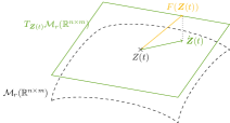
Figure 1: Orthogonal projection on the tangent space $T_{Z(t)}\mathcal{M}_{r}({\mathbb{R}^{n\times m}})$.

In view of MOR, the goal of low-rank methods is to approximate the solution $A(t)$ of Equation (1) with $Z(t)$ solution of Equation (4) which is cheaper to compute. However, in practice additional difficulties appear for the numerical integration of Equation (4).
The first difficulty relies on the proper description of the manifold of fixed rank matrices $\mathcal{M}_{r}(\mathbb{R}^{n\times m})$. In practice, a way to compute the rank-$r$ matrix $Z(t)$ is done through its parametrization

$$Z(t)=U(t)G(t)V(t)^{T},$$ (5)

with $U(t)\in\mathbb{R}^{n\times r},V(t)\in\mathbb{R}^{m\times r}$ and $G(t)\in\mathbb{R}^{r\times r}$. Such a parametrization of the matrix $Z(t)$ is not unique. A way to dodge this undesirable property is to properly define the tangent space $T_{Z(t)}\mathcal{M}_{r}({\mathbb{R}^{n\times m}})$. Given $Z(0)=U(0)G(0)V(0)^{T}$, the matrix $Z(t)$ admits a unique decomposition of the form (5) when imposing the so-called gauge conditions on $U,V$ (see [14, Proposition 2.1]). In addition, the system (4) results in a system ODEs driving the evolution of the parameters $U,G,V$.
The second difficulty appears when numerical integration is performed for solving the resulting system of ODEs governing the evolution of parameters $U,V$ and $G$. Indeed in presence of small singular values for $Z(t)$, the matrix $G(t)$ may be ill-conditioned. As consequence, classical integration schemes may be unstable (see e.g. [11, Section 2.1]). Moreover, in case of overapproximation, i.e. when the approximation $Z(t)$ has a rank $r$ greater than the rank of the exact solution $A(t)$, these method fails since $G(t)$ becomes singular. A possible way to address this issue is regularize $G$ such that it remains invertible. Nevertheless, it has the drawback to modify the problem (then the approximate solution) and does not prevent ill-conditioning of $G(t)$. In [15] an explicit projection-splitting integrator is proposed to deal with numerical integration of (4). It is based on a Lie-Trotter splitting of the projection operator $P_{T_{Z(t)}}$. In addition to its simplicity, it has the advantage to remains robust in case of small singular values and especially for overapproximation as it avoids the inversion of $G(t)$. The resulting method is fully explicit and first order, extension to second order via Strang splitting scheme could be considered. Variants of this algorithm have been proposed in [4] to integrate some symmetry properties. More recently in [5], the authors derive a different robust algorithm for dynamical low-rank approximation. When interested in higher order approximation, projection based methods [12], in the lines of Riemaniann optimization, combined to explicit Runge-Kutta schemes could be considered. Such methods work as follows. Perform one step of the numerical scheme leaving the manifold, and then project on the manifold by means of retraction. The latter step is usually performed using a $r$-terms truncated SVD.

In [3], the authors give a different geometric description of the fixed-rank matrix manifold and the associated tangent space. This description combines a natural definition of the neighborhood of $Z$ together with explicit description of local charts such that the set $\mathcal{M}_{r}(\mathbb{R}^{n\times m})$ is endowed with the structure of analytic principal bundle [3, Theorem 4.1]. Moreover, it ensures that any matrix in the neighborhood of a matrix $Z$ (including itself) admits a unique representation in the form $UGV^{T}$. The main contribution of this paper is twofold. First, we revisit dynamical low-rank approximation by using the geometric description of the matrix manifold given in [3]. The resulting system of ODEs on the parameters is shown to be related to the one obtained in [14] but with no need of gauge conditions. Secondly, relying on this geometric description of $\mathcal{M}_{r}(\mathbb{R}^{n\times m})$, we derive a first order numerical integrator in local coordinates for solving (4) that can be interpreted as a splitting integrator. It is proven to coincide with the so-called KSL splitting algorithm introduced in [15] in the particular case where the flux $F$ only depends on $t$.

The outline of the paper is as follows. We detail in Section 2 the proposed geometric description of the manifold of rank-$r$ matrices. In Section 3 we describe a new splitting algorithm relying on the proposed geometric description Finally, in Section 4, we confront the proposed splitting algorithm to KSL splitting integrator [15] on several numerical test cases.

2 Dynamical low-rank approximation: a geometric approach

Dynamical low-rank approximation consists in approximating at each time $t$ the matrix $A(t)$ by a matrix $Z(t)\in\mathcal{M}_{r}(\mathbb{R}^{n\times m})$ that can be represented (in non-unique way) by means of the factorization

$$Z=UGV^{T},$$

with $U\in\mathcal{M}_{r}(\mathbb{R}^{n\times r}),V\in\mathcal{M}_{r}(\mathbb{R}^{m\times r})$ and $G\in\mathrm{GL}_{r}$ with $\mathrm{GL}_{r}$ the Lie group of $r\times r$ invertible matrices. We present in Section 2.1 a geometric description of $\mathcal{M}_{r}(\mathbb{R}^{n\times m})$. We restrict the presentation to essential elements of geometry required thereafter. The interested reader could consult the original paper [3] for further details. In Section 2.2 we discuss the interest of the proposed description for dynamical low-rank approximation. Finally, we draw the link with the geometric description proposed in [14] in Section 2.3.

2.1 Chart based geometric description of $\mathcal{M}_{r}(\mathbb{R}^{n\times m})$

Let $Z=UGV^{T}\in\mathcal{M}_{r}(\mathbb{R}^{n\times m})$. We consider $U_{\bot}\in\mathcal{M}_{n-r}(\mathbb{R}^{n\times(n-r)}),V_{\bot}\in\mathcal{M}_{m-r}(\mathbb{R}^{n\times(m-r)}),$ the matrices such that $U_{\perp}^{T}U=0$ and $V_{\perp}^{T}V=0$. The neighborhood ${\cal U}_{Z}$ of $Z$ in $\mathcal{M}_{r}(\mathbb{R}^{n\times m})$ is defined as the set

$${\cal U}_{Z}=\{(U+U_{\perp}X)H(V+V_{\bot}Y)^{T}:(X,Y,H)\in\mathbb{R}^{(n-r)\times r}\times\mathbb{R}^{(m-r)\times r}\times\mathrm{GL}_{r}\}.$$

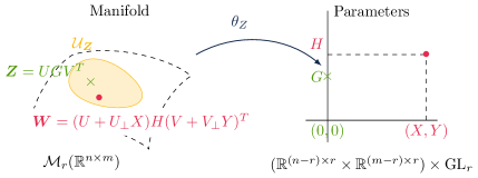
Figure 2: Representation of the local chart $\theta_{Z}$ that associates to $W=(U+U_{\perp}X)H(V+V_{\perp}Y)^{T}$ in ${\cal U}_{Z}\subset\mathcal{M}_{r}(\mathbb{R}^{n\times m})$ the parameters $(X,Y,H)\in\mathbb{R}^{(n-r)\times r}\times\mathbb{R}^{(m-r)\times r}\times\mathrm{GL}_{r}$ .

We associate to the neighborhood ${\cal U}_{Z}$ of $Z$ the local chart $\theta_{Z}:{\cal U}_{Z}\to\mathbb{R}^{(n-r)\times r}\times\mathbb{R}^{(m-r)\times r}\times\mathrm{GL}_{r}$ (see Figure 2) which is given by

$$\theta_{Z}(W)=(U_{\bot}^{+}W(V^{+})^{T}(U^{+}W(V^{+})^{T})^{-1},V_{\bot}^{+}W^{T}(U^{+})^{T}(V^{+}W^{T}(U^{+})^{T})^{-1},U^{+}W(V^{+})^{T})$$

for any $W\in\mathcal{U}_{Z}$. Here $U^{+}$ and $V^{+}$ stand for the Moore-Penrose pseudo-inverses of $U$ and $V$ respectively. This means that any matrix $W$ belonging to the neighborhood ${\cal U}_{Z}$ admits a unique parametrization

$$W=\theta_{Z}^{-1}(X,Y,H),$$

with parameters $(X,Y,H)\in\mathbb{R}^{(n-r)\times r}\times\mathbb{R}^{(m-r)\times r}\times\mathrm{GL}_{r}$ and where the map $\theta_{Z}^{-1}$ is defined by

$$\theta_{Z}^{-1}(X,Y,H)=(U+U_{\bot}X)H(V+V_{\bot}Y)^{T}.$$

In this description, the parameters are not longer $U,V,G$ but $X,Y,H$. Note that $\theta_{Z}^{-1}(0,0,G)=Z$.

Such geometric description confers the set $\mathcal{M}_{r}(\mathbb{R}^{n\times m})$ the structure of an analytic manifold and of a principal bundle [3, §4].

Proposition 2.1.

The set of fixed rank matrices $\mathcal{M}_{r}(\mathbb{R}^{n\times m})$ equipped with the atlas ${\cal A}_{n,m,r}=\{({\cal U}_{Z},\theta_{Z}):Z\in\mathcal{M}_{r}(\mathbb{R}^{n\times m})\}$ is an analytic $r(n+m-r)$-dimensional manifold modelled on $\mathbb{R}^{(n-r)\times r}\times\mathbb{R}^{(m-r)\times r}\times\mathbb{R}^{r\times r}$. Moreover $\mathcal{M}_{r}(\mathbb{R}^{n\times m})$ is an analytic principal bundle with typical fiber $\mathrm{GL}_{r}$ and base $\mathbb{G}_{r}(\mathbb{R}^{n})\times\mathbb{G}_{r}(\mathbb{R}^{m})$.

We now give a description of the tangent space to the manifold of rank-$r$ matrices at $Z$ denoted $T_{Z}\mathcal{M}_{r}(\mathbb{R}^{n\times m})$.

To that goal, we define the tangent map at $Z\in\mathcal{M}_{r}(\mathbb{R}^{n\times m})$ noted $\mathrm{T}_{Z}{i}$ by

$$\mathrm{T}_{Z}{i}:\mathbb{R}^{(n-r)\times r}\times\mathbb{R}^{(m-r)\times r}\times\mathbb{R}^{r\times r} \rightarrow\mathbb{R}^{n\times m},$$

$$(\delta X,\delta Y,\delta H) \mapsto U_{\bot}\delta XGV^{T}+UG(V_{\bot}\delta Y)^{T}+U\delta HV^{T}.$$

Then, the tangent space to $\mathcal{M}_{r}(\mathbb{R}^{n\times m})$ at $Z$ is defined as the image through $\mathrm{T}_{Z}{i}$ of the tangent space in the local coordinates in $\mathbb{R}^{(n-r)\times r}\times\mathbb{R}^{(m-r)\times r}\times\mathbb{R}^{r\times r}$

$${T}_{Z}\mathcal{M}_{r}(\mathbb{R}^{n\times m}) =\{U_{\bot}\delta XGV^{T}+UG(V_{\bot}\delta Y)^{T}+U\delta GV^{T}:\delta X\in\mathbb{R}^{(n-r)\times r},\delta Y\in\mathbb{R}^{(m-r)\times r},\delta G\in\mathbb{R}^{r\times r}\}.$$

As stated in [3, Proposition 4.3], $\mathrm{T}_{Z}i$ is an isomorphism between $T_{Z}\mathcal{M}_{r}(\mathbb{R}^{n\times m})$ and $\mathbb{R}^{(n-r)\times r}\times\mathbb{R}^{(m-r)\times r}\times\mathbb{R}^{r\times r}$.

Proposition 2.2.

The tangent map $\mathrm{T}_{Z}i$ at $Z$ is a linear isomorphism with inverse $(\mathrm{T}_{Z}{i})^{-1}$ given by

$$(\mathrm{T}_{Z}{i})^{-1}(\delta W)=(U_{\bot}^{+}\delta W(V^{+})^{T}G^{-1},V_{\bot}^{+}\delta W^{T}(U^{+})^{T}G^{-T},U^{+}\delta W(V^{+})^{T})$$

for $\delta W\in\mathbb{R}^{n\times m}$.

By Proposition 2.2, any tangent matrix $\delta Z\in T_{Z}\mathcal{M}_{r}(\mathbb{R}^{n\times m})$ admits a unique parametrization of the form

$$\delta Z=\mathrm{T}_{Z}{i}(\delta X,\delta Y,\delta H)=U_{\perp}\delta XGV^{T}+UG(V_{\perp}\delta Y)^{T}+U\delta HV^{T},$$ (6)

where $(\delta X,\delta Y,\delta H)\in\mathbb{R}^{(n-r)\times r}\times\mathbb{R}^{(m-r)\times r}\times\mathbb{R}^{r\times r}$ are uniquely given through

$$\begin{array}[]{rcl}\delta X&=&U_{\perp}^{+}\delta Z(V^{+})^{T}G^{-1},\\ \^{A}~\delta Y&=&V_{\perp}^{+}\delta Z^{T}(U^{+})^{T}G^{-T},\\ \^{A}~\delta H&=&U^{+}\delta Z(V^{+})^{T}.\end{array}$$ (7)

Remark 2.3.

The tangent space could be decomposed into distinct pieces which are the vertical tangent space

$${T}_{Z}^{V}\mathcal{M}_{r}(\mathbb{R}^{n\times m})=\{U\delta GV^{T}:\delta G\in\mathbb{R}^{r\times r}\},$$

and the horizontal tangent space

$${T}_{Z}^{H}\mathcal{M}_{r}(\mathbb{R}^{n\times m})=\{U_{\bot}\delta XGV^{T}+UG(V_{\bot}\delta Y)^{T}:\delta X\in\mathbb{R}^{(n-r)\times r},\delta Y\in\mathbb{R}^{(m-r)\times r}\},$$

where ${T}_{Z}^{V}\mathcal{M}_{r}(\mathbb{R}^{n\times m})$ is associated to the fiber and ${T}_{Z}^{H}\mathcal{M}_{r}(\mathbb{R}^{n\times m})$ to the base.

2.2 Dynamical low-rank approximation

In the context of dynamical low-rank approximation, we recall that $Z$ is given through the projected Equation (4). By definition of the tangent space (6), the tangent matrix is given by $\dot{Z}=\mathrm{T}_{Z}{i}(\dot{X},\dot{Y},\dot{H})$ where the parameters satisfies

$$(\dot{X},\dot{Y},\dot{H})=\mathrm{T}_{Z}{i}^{-1}\left(P_{T_{Z}}F(Z)\right)$$ (8)

with

$$P_{T_{Z}}F(Z)=P_{U}^{\perp}F(Z)P_{V}^{T}+P_{U}^{T}F(Z)(P_{V}^{\perp})^{T}+P_{U}F(Z)P_{V}^{T}.$$

Here $P_{U}=UU^{+},P_{V}=VV^{+}$ denote the projections associated to $U,V$ respectively, and their related orthogonal projections $P_{U}^{\perp}=I-P_{U}$, $P_{V}^{\perp}=I-P_{V}$. Equation (8) yields equivalently to the following system of ODEs on the parameters:

$$\begin{array}[]{rcl}\dot{X}&=&U_{\perp}^{+}F(Z)(V^{+})^{T}G^{-1},\\ \^{A}~\dot{Y}&=&V_{\perp}^{+}F(Z)^{T}(U^{+})^{T}G^{-T},\\ \^{A}~\dot{H}&=&U^{+}F(Z)(V^{+})^{T}.\end{array}$$ (9)

The proposed geometrical description ensures that (8) admits a unique maximal solution $Z$ when the original problem is an autonomous dynamical system with vector field $F$ [7, Theorem 2.6, Theorem 3.5]

Proposition 2.4.

Assume $F:\mathbb{R}^{n\times m}\to\mathbb{R}^{n\times m}$ is a ${\cal C}^{p}$ vector field. Then (1) admits a unique solution. Moreover, $\mathrm{T}_{Z}{i}^{-1}P_{T_{Z}}F:\mathbb{R}^{n\times m}\to\mathbb{R}^{(n-r)\times r}\times\mathbb{R}^{(m-r)\times r}\times\mathbb{R}^{r\times r}$ is a ${\cal C}^{p}$ vector field which ensures that the dynamical system (8) also admits a unique solution.

2.3 Link with the geometric description introduced in [14].

In this section, we discuss the relation between the proposed geometric approach and the description introduced in [14] . In the latter, the non-uniqueness of the parametrization $Z=UGV^{T}$ is avoided by computing the tangent matrix $\delta Z$ in $T_{Z}\mathcal{M}_{r}(\mathbb{R}^{n\times m})$. Introducing

$$\delta Z=\delta UGV^{T}+U\delta GV^{T}+UG\delta V^{T}$$ (10)

together with the gauge conditions

$$U^{T}\delta U=0\text{ and }\^{A}~V^{T}\delta V=0,$$ (11)

and assuming that $U,V$ are orthogonal, then the parameter derivatives $\delta U,\delta G,\delta V$ are uniquely given [14, Proposition 2.1] by

$$\begin{array}[]{rcl}\delta U&=&(I-UU^{T})\delta ZVG^{-1},\\ \^{A}~\delta V&=&(I-VV^{T})\delta Z^{T}UG^{-T},\\ \^{A}~\delta G&=&U^{T}\delta ZV.\end{array}$$ (12)

This can be interpreted as constructing an isomorphism between

$$T_{Z}\mathcal{M}_{r}(\mathbb{R}^{n\times m})~{}\^{A}~\text{ and }\{(\delta G,\delta U,\delta V)\in\mathbb{R}^{n\times r}\times\mathbb{R}^{m\times r}\times\mathbb{R}^{r\times r}:U^{T}\delta U=0,V^{T}\delta V=0\}.$$

The geometric description proposed in Section 2.1 allows to recover (10)-(12). Indeed, by setting $(\delta U,\delta V,\delta G)=(U_{\perp}\delta X,V_{\perp}\delta Z,\delta H)$ in the definition (6) of the tangent matrix $\delta Z$, we get (10). Moreover, the gauge conditions are naturally satisfied as $U^{T}\delta U=U^{T}U_{\perp}\delta X=0,V^{T}\delta V=V^{T}V_{\perp}\delta Z=0$. Finally, for $U,V$ orthogonal we have $UU^{+}=UU^{T},VV^{+}=VV^{T}$ and by multiplying the first and second equations of (7) by $U_{\perp}$ and $V_{\perp}$ respectively we recover (12).

Going back to dynamical low-rank approximation, when $Z$ corresponds to the rank-$r$ approximation of a matrix $A$ through Equation (4), we get from (12) the following system of ODEs governing the evolution of the factors $U,G,V$,

$$\begin{array}[]{rcl}\dot{U}&=&(I-UU^{T})F(Z)VG^{-1},\\ \^{A}~\dot{V}&=&(I-VV^{T})F(Z)^{T}UG^{-T},\\ \^{A}~\dot{G}&=&U^{T}F(Z)V.\end{array}$$ (13)

Again, this system can be deduced from (9) by setting $(\dot{U},\dot{V},\dot{G})=(U_{\perp}\dot{X},V_{\perp}\dot{Z},\dot{H})$ and assuming that $U,V$ orthogonal.

3 Projection splitting integrator schemes

In this section, we derive suitable schemes for numerical integration of the projected equation (4). Two splitting methods are presented, first in an abstract semi-discretized framework in Section 3.1 and then in their practical form in Section 3.2. Then, the relation between these two practical algorithms is discussed.

3.1 Splitting integrators

3.1.1 Symmetric splitting method

We first consider the setting of the classical description [14] detailed in Section 2.3. To perform time integration, a symmetric Lie-Trotter splitting method [15] is applied to Equation (3). This integration scheme relies on a decomposition of the projection $P_{T_{Z}(t)}$ as follows

$$P_{T_{Z}(t)}={Q}_{1}-{Q}_{2}+{Q}_{3},$$ (14)

where ${Q}_{1}$, ${Q}_{2}$ and ${Q}_{3}$ are three projections respectively defined by

$${Q}_{1}A=AP_{V}^{T},\quad{Q}_{2}A=P_{U}AP_{V}^{T},\quad{Q}_{3}A=P_{U}A,$$ (15)

for any $A\in\mathbb{R}^{n\times m}$. Note that this splitting is not associated to a direct sum decomposition of the tangent space. Using this splitting, one integration step from $t_{0}$ to $t_{1}$ starting from the factorized rank-$r$ matrix $Z_{0}=Z(t_{0})$ under the form $Z_{0}=U_{0}G_{0}V_{0}^{T}$ reads as follows.

1. Integrate on $[t_{0},t_{1}]$ the $n\times r$ matrix differential equation

   $$\dfrac{d}{dt}(UG)=F((UG)V^{T})V,\quad\dot{V}=0,$$

   with initial conditions $(UG)(t_{0})=U_{0}G_{0}$, $V(t_{0})=V_{0}.$ Then set $U_{1}$ and $\hat{G}_{1}$ such that $U_{1}\hat{G}_{1}=(UG)(t_{1})$.

2. Integrate on $[t_{0},t_{1}]$ the $r\times r$ matrix differential equation

   $$\dot{G}=-U^{T}F(UGV^{T})V,\quad\dot{U}=0,\quad\dot{V}=0,$$

   with initial conditions $G(t_{0})=\hat{G}_{1}$, $U(t_{0})=U_{1}$, $V(t_{0})=V_{0}.$ Set $\tilde{G}_{1}=G(t_{1})$.

3. Integrate on $[t_{0},t_{1}]$ the $m\times r$ matrix differential equation

   $$\dfrac{d}{dt}(VG^{T})=F(U(VG^{T})^{T})^{T}U,\quad\dot{U}=0,$$

   with initial conditions $(VG)^{T}(t_{0})=V_{0}\tilde{G}_{1}^{T}$, $U(t_{0})=U_{1}$. Set $V_{1}$ and $G_{1}$ such that $V_{1}G_{1}^{T}=(VG^{T})(t_{1})$.

After these steps, the obtained approximation is $Z(t_{1})=U_{1}G_{1}V_{1}^{T}$. Each step corresponds to the integration of the right hand side of (4) associated to the projections $Q_{1}$, $Q_{2}$ and $Q_{3}$ respectively (for details see [15, Lemma 3.1]).

Remark 3.1.

This splitting algorithm works in the following order. First, it updates $UG$, then $G$ and finally $VG$. As we will discuss in Section 3.2, this particular choice allows to recover exactness properties of the splitting scheme in the context of matrix approximation [15].

Remark 3.2.

The inversion of $G$ is avoided. This convenient choice allow to deal with the case of over-approximation, in i.e. when the rank of the approximation $Z$ is smaller then $r$.

3.1.2 Chart based splitting method

The second contribution of this paper is to propose a numerical integrator relying on the fibre bundle structure of the manifold of fixed rank matrices proposed in Section 2.

Based on the chart description of Section 2.2, the guiding idea is to perform some update of the parameters $(X,Y,H)$, instead of $(U,G,V)$ directly, whose dynamic is governed by the system of ODEs (9). Working in a fixed neighborhood ${\cal U}_{Z}$ of $Z$, the matrices $U,V,G$ are fixed and Equation (9) writes equivalently

$$\begin{array}[]{rcl}\dot{H}&=&U^{+}F(Z)(V^{+})^{T},\\[5.69046pt] \dot{X}G&=&{U}_{\perp}^{+}F(Z)(V^{+})^{T},\\[5.69046pt] \dot{Y}G^{T}&=&{V}_{\perp}^{+}F(Z)^{T}(U^{+})^{T}.\end{array}$$ (16)

Then, we integrate the system (16) from $t_{0}$ to $t_{1}$ in three steps. Letting $U(t)=U(t_{0})+U(t_{0})_{\perp}X(t)$, $V(t)=V(t_{0})+V(t_{0})_{\perp}Y(t)$ and $Z(t)=U(t)H(t)V(t)^{T}$, we start from $(X(t_{0}),Y(t_{0}),H(t_{0}))=(0,0,G(t_{0}))$ and we proceed as follows.

1. Integrate on $[t_{0},t_{1}]$ the $r\times r$ matrix differential equation

   $$\dot{H}=U^{+}F(Z)(V^{+})^{T},\;\dot{X}=0,\quad\dot{Y}=0,$$

   with initial conditions $X(t_{0})=0,H(t_{0})=G(t_{0})$ and $Y(t_{0})=0$. Set $H_{1}=H(t_{1})$.

2. Integrate on $[t_{0},t_{1}]$ the $n\times r$ matrix differential equation

   $$\dot{X}H=U_{\perp}^{+}F(Z)(V^{+})^{T},\quad{\dot{H}=0},\quad\dot{Y}=0,$$

   with initial conditions $X(t_{0})=0,H(t_{0})=H_{1}$ and $Y(t_{0})=0$. Then set $X_{1}=X(t_{1})$.

3. Integrate on $[t_{0},t_{1}]$ the $m\times r$ matrix differential equation

   $$\dot{Y}H^{T}=V_{\perp}^{+}F(Z)^{T}(U^{+})^{T},\quad{\dot{H}=0},\quad\dot{X}=0.$$

   with initial conditions $X(t_{0})=X_{1},H(t_{0})=H_{1}$ and $Y(t_{0})=0$. Then set $Y_{1}=Y(t_{1})$.

After these three steps, we obtain an approximation $Z(t_{1}):=U_{1}H_{1}V_{1}^{T}$ with $U_{1}=U(t_{0})+U(t_{0})_{\perp}X_{1}$ and $V_{1}=V(t_{0})+V(t_{0})_{\perp}Y_{1}$.

In the lines of the previous method (see Section 3.1.1), the chart based method can be interpreted as a Lie-Trotter splitting that relies on the following decomposition of the projection

$$P_{T_{Z}(t)}={P}_{1}+{P}_{2}+{P}_{3},$$ (17)

where ${P}_{1}$, ${P}_{2}$ and ${P}_{3}$ are three projections respectively defined by

$${P}_{1}A=P_{U}AP_{V}^{T},\quad{P}_{2}A=P_{U}^{\perp}AP_{V}^{T},\quad{P}_{3}A=P_{U}A(P_{V}^{\perp})^{T},$$ (18)

for any $A\in\mathbb{R}^{n\times m}$. Note that, contrary to the symmetric splitting method, the proposed splitting follows from a direct sum decomposition of the tangent space. Here each term $P_{i}$ of the projection is associated to the ODE solved at Step $i$. This point is discussed and detailed in the Appendix A.

Remark 3.3.

As for the splitting method of Section 3.1.1, we avoid the inversion of matrix $G$ which allows to deal with overapproximation case where $H$ is singular.

Remark 3.4.

The symmetric splitting and the chart based methods differ by the update order. Indeed, the chart based method first updates $H$ and then $X,Y$ (or equivalently $G$ and then $U,V$). Moreover, Step 2 of the symmetric splitting method described in Section 3.1.1 can be interpreted as a backward evolution problem that can be ill-conditionned, as pointed out in [1, Section 5]. In the chart based method, the update of $G$ at Step 1 is still a forward evolution problem due to our splitting choice. Let us mention that other integration strategies have been recently proposed in [1, 5].

3.2 Practical algorithms

Now, we provide practical formulation of those methods amenable for numerical use. To that goal, let introduce preliminary notations. We consider a uniform discretization of the time interval $[0,T]$, $T>0$, containing $K+1$ nodes $0=t^{0}<t^{1}<t^{2}<\dots<t^{K}$ where $t^{k}=k\Delta t$ and $\Delta t=\frac{T}{K}$. The matrix $Z^{k}$ is the approximation at each time step $t^{k}$ of $Z$ computed on $[t_{0},t_{1}]=[t^{k},t^{k+1}]$ through the splitting methods given in Section 3.1. Explicit approximation of the flux is performed leading the schemes summarized in the following algorithms.

Following the previous sections, we first introduce the KSL Algorithm (see Algorithm 3.5) for the symmetric splitting scheme. Here, we adopt the original name given in [15], with the following correspondence: $K$ stands for $UG$, $S$ for $G$ and $L$ for $VG^{T}$.

Algorithm 3.5 (KSL algorithm).

Given the initial rank-$r$ approximation $Z^{0}=U^{0}G^{0}(V^{0})^{T}$, compute $Z^{k}\in\mathcal{M}_{r}(\mathbb{R}^{n\times m})$ for $k\in\{1,...,K\}$ as follows.

• Start with $U_{0}=U^{k-1},G_{0}=G^{k-1}$ and $V_{0}=V^{k-1}$.

  1. Set

     $$(UG)_{1}=U_{0}G_{0}+\Delta tF(Z_{0},t^{k-1})V_{0}$$

     and $U_{1}$ and $\hat{G}_{1}$ such that $U_{1}\hat{G}_{1}=(UG)_{1}$ (computed using QR).

  2. Set

     $$\tilde{G}_{1}=\hat{G}_{1}-\Delta tU_{1}^{T}F(U_{1}\hat{G}_{1}V_{0}^{T},t^{k-1})V_{0}.$$

  3. Set

     $$(VG^{T})_{1}=V_{0}\tilde{G}_{1}^{T}+\Delta tF(U_{1}\tilde{G}_{1}V_{0}^{T},t^{k-1})^{T}U_{1}^{T}$$

     and $V_{1}$ and $G_{1}$ such that $V_{1}G_{1}^{T}=(VG^{T})_{1}$ (computed using QR).

• Set $Z^{k}=U_{1}G_{1}V_{1}^{T}$.

Now, we give the chart based algorithm (see Algorithm 3.6) relying on the splitting introduced in Section 3.1.2.

Algorithm 3.6 (Chart based algorithm).

Given the initial rank-$r$ approximation $Z^{0}=U^{0}G^{0}(V^{0})^{T}$, compute $Z^{k}\in\mathcal{M}_{r}(\mathbb{R}^{n\times m})$ for $k\in\{1,...,K\}$ as follows.

• Set $U_{0}=U^{k-1},V_{0}=V^{k-1}$ and $H_{0}=G^{k-1}$.

  1. Set

     $$\hat{H}_{1}=H_{0}+\Delta t(U_{0})^{+}F(U_{0}G_{0}V_{0}^{T},t^{k-1})(V_{0}^{+})^{T}.$$

  2. Set

     $$(XH)_{1}=\Delta t\,{U_{0}}_{\perp}^{+}F(U_{0}\hat{H}_{1}V_{0}^{T},t^{k-1})(V_{0}^{+})^{T}$$

     and $U_{1}$ and $\tilde{H}_{1}$ such that $U_{1}\tilde{H}_{1}=U_{0}\hat{H}_{1}+U_{0,\perp}(XH)_{1}$ (computed using QR).

  3. Set

     $$(YH^{T})_{1}=\Delta t\,{V_{0}}_{\perp}^{+}F(U_{1}\tilde{H}_{1}V_{0}^{T},t^{k-1})^{T}(U_{1}^{+})^{T},$$

     and $V_{1}$ and $H_{1}$ such that ${V_{1}H_{1}^{T}}=V_{0}\tilde{H}_{1}^{T}+V_{0,\perp}(YH^{T})_{1}$ (computed using QR).

• Set $Z^{k}=U_{1}H_{1}V_{1}^{T}$.

Remark 3.7.

For numerical stability, updates of $U$ and $V$ are performed with $QR$ factorization in both algorithms. Note that $SVD$ should have been considered instead.

Remark 3.8.

From practical point of view, the new algorithm is very similar to the KSL algorithm in its implementation. The only practical differences are in the order of the update and the sign in the update of $G$ at Step 1, as discussed in Remark 3.4.

Remark 3.9.

The proposed practical algorithms are only first order splitting methods. Higher order extensions should be considered in the line of [15, Section 3.3.].

Remark 3.10.

In the chart based algorithm, matrices ${U_{0}}_{\perp}$ and ${V_{0}}_{\perp}$ are not computed explicitly in practice. Indeed, we directly compute $U_{0,\perp}(XH)_{1}$ and $V_{0,\perp}(YH^{T})_{1}$ that only requires the calculation of $P_{U_{0}}^{\perp}=U_{0,\perp}U_{0,\perp}^{+}=I-P_{U_{0}}$ and $P_{V_{0}}^{\perp}=V_{0,\perp}V_{0,\perp}^{+}=I-P_{V_{0}}$.

Link between the two practical algorithms

Here, we discuss the similarity of the two proposed practical algorithms in the particular case where the flux $F$ is independent of $Z$ which includes the particular case of matrix approximation where $F(Z(t),t):=\dot{A}(t)$ with $A(t)\in\mathbb{R}^{n\times m}$.

Lemma 3.11.

In the case where the flux $F$ is independent of $Z$ meaning $F(Z(t),t):=F(t),$ the sequence of approximations $\{Z^{k}\}_{k}\subset\mathcal{M}_{r}(\mathbb{R}^{n\times m})$ provided by KSL algorithm and chart based algorithm coincide.

Proof.

We assume that the explicit flux evaluation $F(t^{k-1})$, required at each time step $k$ of both KSL and chart based algorithms, is noted $F^{k-1}$ for the sake of presentation. For the sake of comparison, the two algorithms are reformulated as follows in term of successive updates on $U,G,V$ and $K,L$. Approximations provided by the chart based algorithm are surrounded by a $\bar{}$ symbol.
At step $k$, the KSL algorithm provides the following approximations

$$K_{1}=U_{0}G_{0}+\Delta tF^{k-1}V_{0}, (U_{1},\hat{G}_{1})=QR(K_{1}),$$ (19)

$$\tilde{G}_{1}=\hat{G}_{1}-\Delta tU_{1}^{T}F^{k-1}V_{0},$$ (20)

$$L_{1}=V_{0}\tilde{G}_{1}^{T}+\Delta t(F^{k-1})^{T}U_{1}, (V_{1},G_{1}^{T})=QR(L_{1}).$$ (21)

Meanwhile, the chart based algorithm gives

$$\bar{\hat{G}}_{1}=G_{0}+\Delta tU_{0}^{T}F^{k-1}V_{0},$$ (22)

$$\bar{K}_{1}=U_{0}\bar{\hat{G}}_{1}+\Delta t(I-P_{U_{0}})F^{k-1}V_{0}, (\bar{U}_{1},\bar{\tilde{G}}_{1})=QR(\bar{K}_{1}),$$ (23)

$$\bar{L}_{1}=V_{0}\bar{\tilde{G}}_{1}^{T}+\Delta t(I-P_{V_{0}})(F^{k-1})^{T}\bar{U}_{1}, (\bar{V}_{1},\bar{G}_{1}^{T})=QR(\bar{L}_{1}).$$ (24)

Expending $\bar{\hat{G}}_{1}$ in Equation (23) yields

$$\bar{K}_{1}=U_{0}\bar{\hat{G}}_{1}+\Delta t(I-P_{U_{0}})F^{k-1}V_{0}=U_{0}G_{0}+\Delta tU_{0}U_{0}^{T}F^{k-1}V_{0}+\Delta t(I-U_{0}U_{0}^{T})F^{k-1}V_{0}=K_{1}.$$

Then $\bar{\tilde{G}}_{1}=\hat{G}_{1}$ and $\bar{U}_{1}=U_{1}$. Using these equalities and injecting the expression of $L_{1}$, we get

$$L_{1}=V_{0}\tilde{G}_{1}^{T}+\Delta t(F^{k-1})^{T}U_{1}=V_{0}\bar{\tilde{G}}_{1}^{T}-\Delta t\bar{V}_{0}\bar{V}_{0}^{T}(F^{k-1})^{T}\bar{U}_{1}+\Delta t(F^{k-1})^{T}\bar{U}_{1}=\bar{L}_{1}$$

from which we deduce $L_{1}=\bar{L}_{1}$ then $G_{1}=\bar{G}_{1}$ and $V_{1}=\bar{V}_{1}$. This implies that $Z^{k}=\bar{Z}^{k}$ which concludes the proof. ∎

In [15], under the assumption that the set of matrices of bounded rank $r$ is an invariant set for the flow, it follows that the KSL method is first order accurate and exact. In consequence, under the same assumptions from Lemma 3.11 the chart based method satisfies the same properties.

Proposition 3.12.

Assume that $A(t)\in\mathbb{R}^{n\times m}$ is a matrix with bounded rank $r$ for all time $t$ and $F(Z(t),t):=\dot{A}(t).$ Setting $\Delta tF(t^{k-1})=A(t^{k})-A(t^{k-1})$, the chart based splitting algorithm is exact, that is, $Z^{k}=A(t^{k}).$

Proof.

The result follows from Lemma 3.11 and the property of exactness of the KSL algorithm [15, Theorem 4.1] in that context. ∎

Remark 3.13.

Proposition 3.12 insures that both methods are exact, whereas they rely on two different splitting methods, with different order of parameter updates. This may sound surprisingly at first, as it has been demonstrated by numerical experiment that [15, §5.2] KLS variant of the KSL algorithm provides less accurate approximations and loses exactness property.

4 Numerical results

In this section, we confront the two presented splitting algorithms namely KSL and chart based algorithms for dynamical low-rank approximation in the context of matrix approximation, in Section 4.1, and matrix dynamical systems arising from a parameter-dependent semi-discretized viscous Burgers’s equation, in Section 4.2.

4.1 Matrix approximation

As first example, we consider the problem of approximating a matrix $A(t)\in\mathbb{R}^{100\times 100}$ on the time interval $[0,1]$. This matrix is given explicitly as

$$A(t)=e^{tW_{1}}De^{t}e^{tW_{2}},$$

where $D$ is a diagonal matrix in $\mathbb{R}^{100\times 100}$ with non zero coefficients $d_{ii}=2^{-i},i\leq 10$, and $W_{1},W_{2}\in$ are two random skew symmetric matrices. Then, $A(t)$ has a rank $10$ whose non zero singular values are $\sigma_{i}(t)=e^{t}2^{-i},i\leq 10$.

The two algorithms are first applied with numerical flux taken equal to $\Delta tF(Z_{i},t^{k-1})=A(t^{k})-A(t^{k-1}),$ where $Z_{i}$ stands for the approximation at Step $i$ of the iteration $k$ of the splitting algorithms. In what follows, we study the behaviour of the approximation error $e^{k}=\|A(t^{k})-Z^{k}\|$ at iteration $k$. Table 1 gives the values of $\max_{k}e^{k}$ for the two methods for $r\in\{10,20\}$. We observe that both methods are exact for $r=10$, which is the rank of the exact solution. In case of over-approximation with $r=20$, the two methods are robust and again provide exact approximation (up to machine precision).

	KSL	chart
$r=10$	$4.03.10^{-15}$	$5.22.10^{-15}$
$r=20$	$5.36.10^{-15}$	$3.77.10^{-15}$

Table 1: Matrix approximation with $\Delta tF(Z_{i},t^{k-1})=A(t^{k})-A(t^{k-1})$: maximum over $k$ of $e^{k}$ for $\Delta t=5~{}\^{A}~10^{-3}$, $r\in\{10,20\}$.

Similar experiments are performed but considering the exact expression of the matrix derivative with $F(Z_{i},t^{k-1})=\dot{A}(t^{k-1})$. Approximation error evolution is depicted on Figure 3.

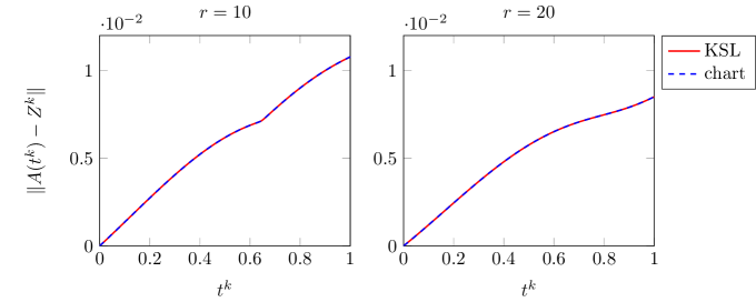
Figure 3: Matrix approximation with $F(Z_{i},t^{k-1})=\dot{A}(t^{k-1})$: evolution of $e^{k}$ for $\Delta t=5~{}\^{A}~10^{-3}$, $r\in\{10,20\}$.

Again, both methods give similar results for $r\in\{10,20\}$, as shown on Figure 3 where the error plots coincide either in case of overapproximation. However, for this choice of $F(Z_{i},t^{k-1})$, both method are no longer exact. Here, the error increases with time up to approximatively $10^{-2}$ with $r=10$ and $10^{-3}$ for $r=20$. To quantify this error, we perform some convergence study with respect to $\Delta t$ and $r$. On Figure 4, we show the behaviour of the final approximation error $e^{K}=\|A(1)-Z^{K}\|$ for various rank $r\in\{4,6,8,16,32\}$ and time step $\Delta t\in\{10^{-5},...,10^{-1}\}$.

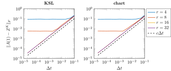
Figure 4: Matrix approximation with $F(Z_{i},t^{k-1})=\dot{A}(t^{k-1})$ : final error $e^{K}$ for both algorithms for different $(r,\Delta t)$.

Figure 4 illustrates that the two methods are first order in time as expected. Indeed we observe a linear decreasing of the error up to some stagnation value for $r\leq 8$. This stagnation is related to the low-rank approximation error as it decreases when $r$ increases.

4.2 Parameter dependent problem

In the lines of [3], we consider the approximation of the parameter-dependent Burger’s viscous equation in one dimension. To that goal, let $\Omega\times I=(0,1)\times[0,1]$ be a space time domain. We seek $u(\cdot;\xi)$ the solution of

$$\partial_{t}u(x,t;\xi)-\mu(\xi)\partial_{xx}^{2}u(x,t;\xi)+{u(t,x;\xi)\partial_{x}u(x,t;\xi)} = f(x,t;\xi),\quad\text{ on }\Omega\times I,$$ (25)

with the initial data $u^{0}(\cdot,\xi):\Omega\to\mathbb{R}$ and supplemented with homogeneous Dirichlet boundary conditions. The solution $u(\cdot;\xi)$ depends on the parameter $\xi\in\mathbb{R}^{3}$ through the viscosity $\mu(\xi)=\xi_{1}$, the initial condition and the source term defined by means of the function $f(\cdot,\cdot;\xi):\Omega\times I\to\mathbb{R}$ given by

$$f(x,t;\xi)=\xi_{2}\exp(-(x-0.2)^{2}/0.03^{2})\sin(\xi_{2}\pi t)\boldsymbol{1}_{[0.1,0.3]}(x).$$

The problem (25) is semi-discretized in space by means of finite difference (FD) schemes with $n$ nodes and $m$ instances of the parameter $\xi$ such that we get the following dynamical system

$$\dot{X}(t)=LX(t)+{h(X,t)},\qquad X(0)=0,$$ (26)

where the solution $X(t)$ is a matrix in $\mathbb{R}^{n\times m}$. The tensorized operator ${L=D_{x}\otimes M_{\xi}}$ is defined by means of $D_{x}\in\mathbb{R}^{n\times n}$ the discrete Laplacian obtained by second order centered FD scheme and $M_{\xi}\in\mathbb{R}^{m\times m}$ a diagonal matrix whose non-zero coefficients are the $m$ instances of $\xi_{1}$. Moreover, we define the matrix valued function $h$ with entries $[h(Z,t)]_{ij}=Z_{ij}[C_{x}Z]_{ij}+f(x_{j},t;\xi_{i})$ where $C_{x}\in\mathbb{R}^{n\times n}$ is the discrete version of the first derivative obtained by 1st order centered FD scheme.

We first confront the KSL and chart based algorithms for solving the discrete parameter dependent Burger’s equation when one single parameter varies. Then, the multiple varying parameter problem is studied.

4.2.1 Single parameter Burger’s problem

In this section, the parameter $\xi_{1}$ takes its values in $[0.01,0.06]$ while the others are fixed to $\xi_{2}=4$ and $\xi_{3}=0$. We chose the following initial condition

$$u^{0}(x;\xi)=sin(x\xi_{1})e^{-100(x-10\xi_{1})^{2}}.$$

and set $n=100$ and $m=60$. For solving the matrix ODE given by Equation (26), we first confront the chart based and KSL algorithms for various ranks, fixing $\Delta t=10^{-4}$. The approximations obtained are compared to a reference solution noted $\{X_{ref}^{k}\}_{k=0}^{K}$ computed with an explicit Euler scheme with $\Delta t=5.10^{-6}$. The time step $\Delta t$ is setting small enough to ensure numerical stability since an explicit integration scheme is applied.

Figure 5 illustrates the behaviour of the numerical solution obtained with the chart based algorithm at final time $t=1$, and $r=20$ for two different instances of the parameter $\xi$.

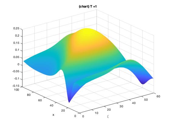
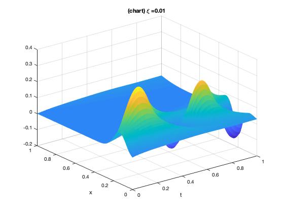
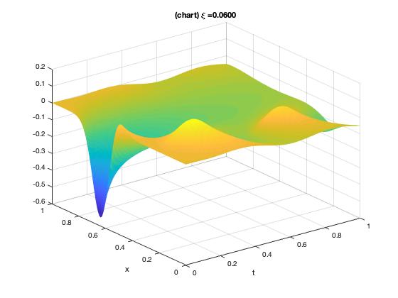
$t=1$	$\xi_{1}=0.01$	$\xi_{1}=0.06$

Figure 5: Burgers’s equation: approximation for the chart method with $r=20$ and $\Delta t=10^{-4}$, at final time $t=1$ (left), for $\xi_{1}=0.01$ (center) and $\xi_{1}=0.06$ (right).

As we can observe on Figure (6), the approximations computed with the two methods are in good agreement with the reference solution.

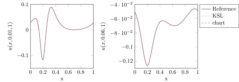
Figure 6: Burgers’s equation: approximation for the chart based and KSL method compared to the reference solution at final time for $r=20$ and $\Delta t=10^{-4}$ .

Now, we compare the approximation error to the reference noted $e^{k}=\|X_{ref}^{k}-Z^{k}\|$ for the two splitting algorithms. On Figure 7, the evolution of $e^{k}$ for both algorithms is studied for different ranks. As we can observe, both methods seem to provide an approximation with similar accuracy, except for ranks $15$ and $20$ where the chart based algorithm provides a slightly more accurate approximation than the KSL algorithm. Note that the error does not necessary increase with respect to time as classically observed for DLR approximation methods which is related to the particular problem considered here.

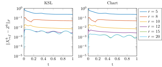
Figure 7: Burgers’s equation: evolution of $e^{k}$ for both algorithms for $r\in\{5,8,10,12,15,20\}$.

This observation is confirmed by Figure 8 where we analyze the convergence with respect to rank and time step. As we can see, the error $e^{K}=\|X_{ref}^{K}-Z^{K}\|$ decreases with respect to the rank and time step, and is the smallest (by up to one order of magnitude) for the chart based algorithm for larger rank.

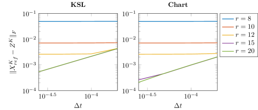
Figure 8: Burgers’s equation: error $e^{K}$ at final time for different $(r,\Delta t)$.

4.2.2 Multiple varying parameters Burger’s problem

To conclude this section, we illustrate the behavior of the two methods for the case where $\xi$ is a vector of independent random parameters uniformly distributed on $[0.01,0.06]\times[2,4]\times[0.01,0.1]$.Here, the initial condition is

$$u^{0}(x;\xi)=\xi_{3}e^{-100(x-10\xi_{2})^{2}}.$$

The numerical simulations are performed for $m=60$ and $n=100$. Here, the two KSL and Chart methods are run with $\Delta t=10^{-4}$ and compared to true numerical reference solution $\{X_{ref}^{k}\}_{k=0}^{K}$ obtained with the explicit Euler scheme with the same time step. The approximation of numerical solution for the Burger’s problem computed with the Chart method with $r=20$ is plotted for two distinct realizations of the parameter $\xi$ showing different features with respect to parameter.

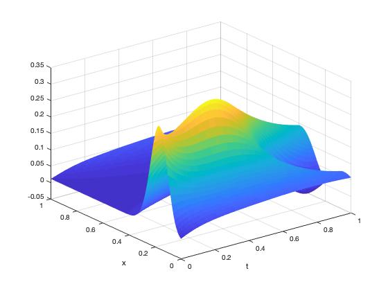
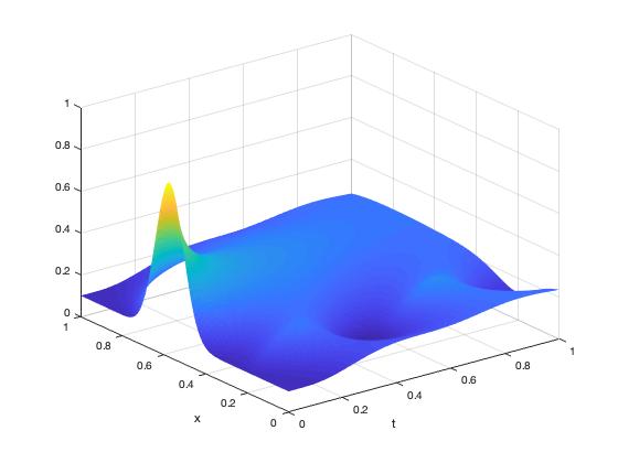
Figure 9: Burgers’s equation: approximation for the chart method with $r=20$ and $\Delta t=10^{-4}$ for two instances of $\xi$.

We represent on Figure 10 the approximation error at final time for the three approaches with respect to $r\in\{5,10,12,15,20,25,30\}$. We clearly observe that the chart method provides a better approximation than KSL for which the error seems to stagnate after $r\geq 12$.

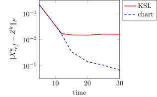
Figure 10: Burgers’s equation (multiple parameter case): error $e^{K}$ at final time for different $r$.

5 Conclusion

In this paper, we have introduced and compared some geometry based algorithms for dynamical low-rank approximation. Using a different geometry description of the set of fixed rank matrices relying on charts, we generalized the description of [14]. Then, from this description we derive a new splitting algorithm motivated by fibre bundle structure of the manifold of fixed rank matrices. The resulting algorithm is proved to coincide with the KSL algorithm [15] in the particular case of matrix approximation. Nevertheless, for more general problems arising from the semi-discretization of parameter-dependent non-linear PDEs, the chart based algorithm seems to outperform the KSL algorithm in some situation. Further work should be conducted for derivation of rigorous error bounds in more general cases as well as high order extension using e.g. Strang splitting variant. Moreover, the proposed splitting scheme is a first step towards designing new algorithms integrating the geometric structure of the manifold of fixed rank matrices, by working in neighborhoods. Especially, deriving a numerical scheme working alternatively in the horizontal and vertical tangent spaces (as pointed out in Remark 2.3) is the object of future research.

Appendix A Chart based splitting integrator

Following the same lines as in [15], we justify how the chart based method introduced in Section 3.1.2 can be interpreted as a splitting scheme relying on the projection decomposition (17) as the sum of three contributions $P_{T_{Z}(t)}=P_{1}+P_{2}+P_{3}$. One integration step of the splitting method starting from $t_{0}$ to $t_{1}$ with initial guess $Z(t_{0})=U(t_{0})G(t_{0})V(t_{0})^{T}$ proceeds as follows.

1. Find $Z\in{\cal U}_{Z(t_{0})}$ on $[t_{0},t_{1}]$ such that $\dot{Z}=P_{U}F(Z)P_{V}^{T}$ with initial condition $Z(t_{0})$.

2. Find $Z\in{\cal U}_{Z(t_{0})}$ on $[t_{0},t_{1}]$ such that $\dot{Z}=P_{U}^{\perp}F(Z)P_{V}^{T}$ with initial condition given by final condition of step (S1).

3. Find $Z\in{\cal U}_{Z(t_{0})}$ on $[t_{0},t_{1}]$ such that $\dot{Z}=P_{U}F(Z)(P^{\perp}_{V})^{T}$ with initial condition given by final condition of step (S2).

At each step (S$i$) of the splitting, $Z$ belongs to the neighborhood of $Z(t_{0})$. Thus it is given by $Z(t)=U(t)H(t)V(t)^{T}$ with $U(t)=U(t_{0})+U(t_{0})_{\perp}X(t)$, $Y(t)=V(t_{0})+V(t_{0})_{\perp}Y(t)$ provided by the ODE solved at Step $i$ of the chart based splitting, as stated in the following proposition.

Proposition A.1.

The solution of (S1) is given by $Z$ with

$$\dot{H}=U^{+}F(Z)V^{T},\quad\dot{X}=0,\quad\dot{Y}=0.$$ (27)

with $H(t_{0})=G(t_{0})$, $X(t_{0})=0$ and $Y(t_{0})=0$. Set

Letting $H_{1}$ be the final condition of $H$ from (S1), the solution of (S2) is given by $Z$ with

$$\dot{X}H={U}_{\perp}^{+}F(Z)(V^{+})^{T},\quad\dot{Y}=0,\quad\dot{H}=0,$$ (28)

with $H(t_{0})=H_{1}$, $X(t_{0})=0$ and $Y(t_{0})=0$. Set $X_{1}=X(t_{1})$.

Letting $X_{1}$ be the final condition of $X$ from (S2), the solution of (S3) is given by $Z$ with

$$\dot{Y}H^{T}={V}_{\perp}^{+}F(Z)(U^{+})^{T},\quad\dot{X}=0,\quad\dot{H}=0,$$ (29)

with $H(t_{0})=H_{1}$, $X(t_{0})=X_{1}$ and $Y(t_{0})=0$.

Proof.

For each step (S$i$), $Z$ admits the decomposition

$$Z=(U(t_{0})+U(t_{0})_{\perp}X)H(V(t_{0})+V(t_{0})_{\perp}Y)^{T}$$

with derivative

$$\dot{Z}=U(t_{0})_{\perp}\dot{X}H(V(t_{0})+V(t_{0})_{\perp}Y)^{T}+(U(t_{0})+U(t_{0})_{\perp}X)\dot{H}(V(t_{0})+V(t_{0})_{\perp}Y)^{T}$$

$$+(U(t_{0})+U(t_{0})_{\perp}X)H(V(t_{0})_{\perp}\dot{Y})^{T}.$$

For (S1), the derivative satisfies $\dot{Z}=P_{U}F(Z)P_{V}^{T}$. Then, multiplying on the left by $U(t_{0})^{+}$ and on the right by $(V(t_{0})^{+})^{T}$ the matrix $\dot{Z}$ in both expressions leads to $\dot{H}=U^{+}F(Z)(V^{+})^{T}$ and $\dot{X}=0,\dot{Y}=0.$
Now let us turn to (S2). The derivative satisfies $\dot{Z}=P_{U}^{\perp}F(Z)P_{V}^{T}$. By multiplying on the right by $(V(t_{0})^{+})^{T}$, the equality is satisfied if $\dot{X}H=U_{\perp}^{+}F(Z)(V^{+})^{T}$ and $\dot{Y}=0,\dot{H}=0.$ The third point of the lemma is obtained from (S3) in the same manner, by multiplying the equation $\dot{Z}=P_{U}F(Z)(P_{V}^{\perp})^{T}$ on the left by $(U(t_{0})+U(t_{0})_{\perp}X_{1})^{+}$ and setting $\dot{X}=0$, $\dot{H}=0$. ∎

References

- [1] Bachmayr M., Eisenmann H., Kieri E., Uschmajew A.: Existence of dynamical low-rank approximations to parabolic problems. Mathematics of Computation, AMS Early View articles, preprint (2021)
- [2] Billaud-Friess M., A. Nouy.: Dynamical model reduction method for solving parameter-dependent dynamical systems. SIAM Journal on Scientific Computing, 39(4), A1766-A1792 (2017)
- [3] Billaud-Friess M. , Falcó A. , Nouy A.: Principal bundle structure of matrix manifolds. arXiv preprint, arXiv:1705.04093 (2017)
- [4] Ceruti G., Lubich C.: Time integration of symmetric and anti-symmetric low-rank matrices and Tucker tensors. arXiv preprint, arXiv:1906.01369 (2019)
- [5] Ceruti G., Lubich C.: An unconventional robust integrator for dynamical low-rank approximation arXiv preprint, arXiv:2010.02022 (2020)
- [6] Cheng M., Hou T.Y., Zhang Z., Sorensen D.-C.:, A dynamically bi-orthogonal method for time-dependent stochastic partial differential equations I: Derivation and algorithms. Journal of Computational Physics, 242(0):843-868 (2013)
- [7] Falcó A., Sánchez F.: Model order reduction for dynamical systems: A geometric approach. Comptes Rendus Mécanique, 346(7), 515-523 (2018)
- [8] Feppon, F., Lermusiaux P.F.J.: A Geometric Approach to Dynamical Model-Order Reduction. SIAM Journal on Matrix Analysis and Applications, 39(1), 510-538 (2018)
- [9] Feppon, F., Lermusiaux P.F.J.: Dynamically Orthogonal Numerical Schemes for Efficient Stochastic Advection and Lagrangian Transport. SIAM Review, 60(3), 595-625, (2018)
- [10] Feppon, F., Lermusiaux P.F.J.: The Extrinsic Geometry of Dynamical Systems Tracking Nonlinear Matrix Projections. SIAM Journal on Matrix Analysis and Applications, 40(2), 814-844 (2019)
- [11] Kieri E., Lubich C., Walach H.: Discretized dynamical low-rank approximation in the presence of small singular values. SIAM Journal on Numerical Analysis, 54(2), 1020-1038 (2016)
- [12] Kieri E., Vandereycken B.:. Projection methods for dynamical low-rank approximation of high-dimensional problems. Computational Methods in Applied Mathematics, 19(1), 73-92 (2019)
- [13] Khoromskij B. N., Oseledets I., Schneider R.: Efficient time-stepping scheme for dynamics on TT-manifolds. preprint (2012).
- [14] Koch O., Lubich C.:. Dynamical low-rank approximation. SIAM Journal on Matrix Analysis and Applications, 29(2), 434-454 (2007)
- [15] Lubich C., Oseledets I. V.: A projection-splitting integrator for dynamical low-rank approximation. BIT Numerical Mathematics, 54(1), 171-188 (2014)
- [16] Musharbash E., Nobile F. Zhou T.: On the dynamically orthogonal approximation of time-dependent random PDEs, SIAM Journal on Scientific Computing, 2015, 37(2):A776-A810 (2015)
- [17] Sapsis T.P., Lermusiaux P.F.J.: Dynamically orthogonal field equations for continuous stochastic dynamical systems. Physica D: Nonlinear Phenomena, 238(23-24):2347–2360 (2009)
- [18] Nonnenmacher A. and C.Lubich C.: Dynamical low-rank approximation: applications and numerical experiments. Mathematics and Computers in Simulation, 79(4), 1346-1357 (2008)