1. Introduction

The definition of a SIC arises naturally in quantum state tomography and in some corners of classical signal processing [1, 2, 3]. It asks for a collection of $d^{2}$ unit vectors forming a resolution of the identity in a complex vector space of dimension $d$, and such that all the absolute values of their mutual scalar products agree. The acronym spells out as “Symmetric Informationally Complete”. All of this sounds simple and harmless, and at first sight it looks as if it should be easy to settle whether SICs exist or not. Numerical investigations strongly suggest that they do, in all dimensions [4, 5].

Since 2016 it is expected that there are infinite sequences of dimensions in which the SICs share number theoretical properties [6]. Moreover there are ample reasons to believe that exact solutions for SICs would look very simple if presented in the right way. But the right way is expected to rely on an unwritten chapter of algebraic number theory, and is not yet known. This makes the SIC existence problem very interesting! Here we will present eight exact solutions in a sequence of dimensions of the form $d=n^{2}+3$. All of them are previously known (see Table 1), but in some cases they have been available only in the form of large txt files. This paper is written for those who like their formulas to be confined to a single page.

To see what property these dimensions share requires a look at the background. Zauner’s conjectures [1], as later refined by Appleby [7] and others, were that in every dimension $d$ SICs exist as orbits under the discrete Weyl–Heisenberg group, and that every such SIC is invariant under a symmetry of order 3. The explicit form of the symmetry is conjectured too. It is one of two types, $F_{z}$ which is realized in all dimensions, and $F_{a}$ which is realized for special SICs in dimensions of the form $d=3\cdot(3k+1)$ [8]. Scott and Grassl [4, 5] conjectured that a SIC invariant under an extra anti-unitary symmetry of order 2 exists in all dimensions of the form $d=n^{2}+3$, $n=1,2,\dots\$. They also conjectured an explicit form of the symmetry.

These conjectures have held up well as new numerical solutions have become available [5], and do suggest that the problem has considerable depth. It turns out that one of our themes, that of algebraic units, is central to the story in more ways than one. Section 2 is intended to explain algebraic units and to sketch the ray class conjecture [6] for SICs. Section 3 explains why SIC symmetries are especially transparent in certain dimensions including the ones we are concerned with. These preparations made we give our exact fiducial vectors in Section 4. They are all located in subfields of the number field needed to construct the full SIC. However, writing down a vector with (say) 52 components necessarily puts a strain on typography, and for this reason five of the solutions are relegated to a five page Appendix. Our conclusions are in Section 5.

Here we want to draw attention to the fact that the vector components can be largely (but not entirely) written in terms of algebraic units. Moreover it seems that these units do have a distinguished status within their respective unit groups. It is already known that units appear as SIC overlap phases [6], and our results point in the same direction even though they are less conclusive. There are good reasons to believe that this may be quite important [9].

2. Algebraic units

Our starting point is the empirical observation [10] that the number fields needed to write down SICs in dimension $d>3$ are abelian extensions of the real quadratic number field ${\mathbb{Q}}(\sqrt{D})={\mathbb{Q}}(\sqrt{D_{0}})$, where

$$D=m^{2}D_{0}=(d+1)(d-3)\ .$$ (1)

Here $m$ is an integer chosen such that $D_{0}$ contains no square factors. Recall that a quadratic number field consists of all expressions of the form $x+y\sqrt{D_{0}}$, where $x,y$ are rational numbers. Making abelian extensions of such number fields raises a non-trivial problem [11], but many insights can be obtained using eq. (1) only. The first question to be addressed is: Given $D_{0}>0$, what are the possible values of $d$?

The first step is to introduce the number $u$ through

$$u=\frac{d-1+\sqrt{D}}{2}\hskip 14.22636pt\Leftrightarrow\hskip 14.22636ptd=1+u+\bar{u}\ .$$ (2)

The Galois conjugate $\bar{x}$ of a number $x\in{\mathbb{Q}}(\sqrt{D})$ is obtained by means of the substitution $\sqrt{D}\rightarrow-\sqrt{D}$, and the norm of $x$ equals $\bar{x}x$. Recall that a number is an algebraic integer if it is a root of a polynomial with integer coefficients and leading coefficient equal to $1$. An algebraic integer is a unit if its inverse is an algebraic integer too. It is easily checked that $u$ is a root of

$$p(t)=(t-u)(t-\bar{u})=t^{2}-(d-1)t+1\ .$$ (3)

Hence it is a unit of norm $\bar{u}u=+1$. A key fact about units is that they form a multiplicative group which is a direct product of a finite cyclic torsion group and a number of infinite cyclic groups. This number is the rank of the unit group. For real quadratic fields the rank of the unit group equals one, and its torsion group consists of $\pm 1$ [12].

It is known that the general solution of eq. (1), regarded as a Diophantine equation for $d$ given $D_{0}$ with $m$ free, is the infinite sequence

$$d_{k}=1+u_{0}^{k}+\bar{u}_{0}^{k}\ ,$$ (4)

where $u_{0}$ is known as the fundamental unit of positive norm [6]. By definition it is the smallest unit larger than 1 and having norm $+1$. This gives rise to a number theoretical connection between SICs in different dimensions. On closer investigation one finds that there are close geometrical ties between the SICs in such sequences, and they illuminate the observations about SIC symmetries that were made by Scott and Grassl [4, 5]. In the absence of a proof of SIC existence for all $d$ the connection remains conjectural, but there are more than one hundred exact solutions all obeying this rule.

The question now arises whether $u_{0}$ is a generator of the unit group. Denote the generator by $\eta_{0}$. There are two possibilities, either $u_{0}=\eta_{0}$ or $u_{0}=\eta_{0}^{2}$. In the latter case the generator has negative norm $\bar{\eta}_{0}\eta_{0}=-1$. A unit $\eta$ of negative norm obeys the minimal polynomial

$$(x-\eta)(x-\bar{\eta})=x^{2}-nx-1=0\ ,$$ (5)

where $n$ is some integer. Solving this equation for $\eta$ and squaring the result we find that

$$\eta=\frac{n+\sqrt{n^{2}+4}}{2}\hskip 14.22636pt\Rightarrow\hskip 14.22636pt\eta^{2}=\frac{n^{2}+2+n\sqrt{n^{2}+4}}{2}\ .$$ (6)

Comparing this with our expression for $u$ in eq. (2) we find that a fundamental unit of negative norm exists if

$$d=n^{2}+3$$ (7)

for some integer $n$. This sequence in a sense ‘connects’ several but not all of the sequences discussed previously. See Figure 1 and Table 1.

Remarkably, based on a fair amount of evidence, Scott and Grassl conjectured that in all these dimensions there exists a SIC with an anti-unitary symmetry of a specified form [4, 5]. Exactly how a number theoretical property—the existence of a fundamental unit with negative norm—implies a geometric property—a symmetry of a SIC—is at the moment enigmatic.

Figure 1. The beginnings of three infinite sequences of related dimensions. Dimensions with more than five digits are not written out. The sequence $d=n^{2}+3$ includes every other dimension in certain special sequences.

The real quadratic field is just the beginning. A much more detailed conjecture [6] concerns the full number field needed to write down SIC vectors in a basis preferred by the Weyl–Heisenberg group. In particular, it is believed that in every dimension $d$ there is a SIC that can be constructed using a ray class field with conductor equal to $d$ if $d$ is odd, and equal to $2d$ if $d$ is even. We will be concerned exclusively with such SICs here. These fields are abelian extensions of the real quadratic field. They have been the subject of much research since Hilbert formulated his 12th problem in the year 1900 [11]. As a result these ray class fields have been completely classified, and there are algorithms (implemented on the computer algebra package Magma) that will provide us with generators for them. However, in most cases we have to do a significant amount of work in order to bring the resulting set of generators into a useful form.

Actually there are four relevant ray class fields, depending on whether they are ramified at any of the two infinite places. Whenever eq. (1) relates the base field and the conductor the degree goes up with a factor of two for each of the two possible ramifications [6]. Number theorists refer to the largest ray class fields as the full ray class fields. We will simply refer to them as “the ray class fields”.

In our small catalogue we have aimed to bring the ray class fields into a form that manifests the symmetry under the Galois transformation $a\leftrightarrow-a$, where $a=\sqrt{D_{0}}$. One reason for doing so is the concrete bridge between the SIC existence problem and the number theoretical Stark conjectures found by Kopp [9]. This bridge rests on exactly this Galois transformation applied to the squared SIC overlaps, although admittedly so far only in the case that $d$ is a prime equal to 2 modulo 3 (as illuminated in a very recent paper [17]).

We will find that algebraic units taken from the ray class fields appear in our exact solutions for SIC vectors. The question then arises how these units are placed within the unit groups of their respective fields (which will now have ranks considerably exceeding one). Unfortunately the available algorithms for calculating the generators of unit groups are very time consuming, and we will be able to offer only scattered comments on this question.

Table 1. The beginning of the sequence of dimensions considered here. The quoted degrees are for ray class fields ramified at both places. The Hilbert class number $h$ is given if it exceeds 1.

$d$	$D_{0}$	Degree of ray class field	Remark	Reference
$4$	5	$16=2^{4}$		[1]
$7$	2	$24=2^{3}\cdot 3$		[7]
$12=4\cdot 3$	13	$64=2^{6}$	$F_{a}$	[8]
$19$	5	$72=2^{3}\cdot 3^{2}$		[7]
$28=4\cdot 7$	29	$576=2^{6}\cdot 3^{2}$		[13]
$39=3\cdot 13$	10	$768=2^{8}\cdot 3$	$F_{a}\ ,\ h=2$	[14]
$52=4\cdot 13$	53	$2304=2^{8}\cdot 3^{2}$		[16]
$67$	17	$2904=2^{3}\cdot 3\cdot 11^{2}$		[16]
$84=4\cdot 3\cdot 7$	85	$4608=2^{9}\cdot 3^{2}$	$F_{a}\ ,\ h=2$	[16]
$103$	26	$13872=2^{4}\cdot 3\cdot 17^{2}$	$h=2$	[16]
$124=4\cdot 31$	5	$2880=2^{6}\cdot 3^{2}\cdot 5$		[15]
$147=3\cdot 7^{2}$	37	$4704=2^{5}\cdot 3\cdot 7^{2}$	$F_{a}$	[16]
$172=4\cdot 43$	173	$28224=2^{6}\cdot 3^{2}\cdot 7^{2}$		[16]
$199$	2	$8712=2^{3}\cdot 3^{2}\cdot 11^{2}$		[16]
$228=4\cdot 3\cdot 19$	229	$62208=2^{8}\cdot 3^{5}$	$F_{a}\ ,\ h=3$	[16]
$259=7\cdot 37$	65	$62208=2^{8}\cdot 3^{5}$	$h=2$	[16]
$292=4\cdot 73$	293	$82944=2^{10}\cdot 3^{4}$		[16]
$327=3\cdot 109$	82	$124416=2^{9}\cdot 3^{5}$	$F_{a}\ ,\ h=4$	[16]
$364=4\cdot 7\cdot 13$	365	$165888=2^{11}\cdot 3^{4}$	$h=2$
$403=13\cdot 31$	101	$86400=2^{7}\cdot 3^{3}\cdot 5^{2}$
$444=4\cdot 3\cdot 37$	445	$331776=2^{12}\cdot 3^{4}$	$F_{a}\ ,\ h=4$

3. Symmetries and dimensions

According to Zauner’s conjecture SICs are generated by a finite Weyl–Heisenberg group acting on some fiducial vector [1]. Unitary or anti-unitary symmetries of SIC vectors come from the Clifford group, which is the group of unitary and anti-unitary operators that permute the elements of the Weyl–Heisenberg group. It is also conjectured that every SIC vector has at least a symmetry of order 3, and the empirical evidence that this is so is by now quite overwhelming [4, 5]. All the group theory that is relevant here is explained in a paper by Appleby [7], except that we will also rely on the Chinese remaindering isomorphism that turns the Clifford group in dimension $d=n_{1}n_{2}$ into a direct product whenever $n_{1}$ and $n_{2}$ are relatively prime [18]. From the number theoretical point of view the single most important point is that the Clifford group can be represented, projectively or faithfully, by matrices whose matrix elements belong to the cyclotomic field ${\mathbb{Q}}(\tau_{d})$, where

$$\tau_{d}=-e^{\frac{\pi i}{d}}\ .$$ (8)

The cyclotomic unit $\tau_{d}$ is always present in the ray class field containing the SIC [6], but it need not be present in every fiducial vector.

A point of considerable importance for us, given our aim to simplify the fiducial vectors as far as we can, is that whenever $d$ is a prime such that $d=3$ or $d=1$ modulo 3 the symmetry of the SIC fiducial can be implemented by monomial matrices. In particular the order 3 Zauner symmetry is then effected by a permutation matrix. This feature was exploited by Appleby when he gave exact solutions in dimensions 7 and 19, and his paper contains a full discussion of this point [7]. It was found later that if the dimension is a square then the entire Clifford group can be represented by monomial matrices, so that the exact solution in dimension 4 can be similarly simplified [18]. We will find both these facts useful, because they cover all the dimensions that we will encounter in our sequence.

Anti-unitary operators involve complex conjugation. When coupled with the preceding remarks this implies that in dimensions that are equal to a prime equal to 1 modulo 3, and for SICs that have an anti-unitary symmetry of order 6, a fiducial vector can be chosen in such a way that is is real [5]. In dimension 4 special measures must be taken to achieve this [18]. Here we have avoided these special measures in order to keep the action of the anti-unitary as transparent as possible.

What kind of dimensions appear in our sequence? We assume that $d=n^{2}+3$. If $n$ is odd $d=4\cdot m$ where $m$ is odd. If $n$ is even $d=m$ is odd. In both cases it holds either that $m=3\cdot k$ or that $m=k$ where $k$ is an odd integer equal to 1 modulo 3. Furthermore the prime decomposition of $k$ can contain only primes equal to 1 modulo 3. To see this, note that we can regard the dimension as the norm of an Eisenstein integer [12]. Recall that $\rho=-1/2+i\sqrt{3}/2$ is a unit in ${\mathbb{Q}}(\sqrt{-3})$. Thus we can write

$$d=n^{2}+3=\left\{\begin{array}[]{lll}(n+i\sqrt{3})\cdot(n-i\sqrt{3})&&\mbox{if $n$ is even}\\ \\ 2^{2}\cdot\left(\frac{n}{2}+\frac{i\sqrt{3}}{2}\right)\cdot\left(\frac{n}{2}-\frac{i\sqrt{3}}{2}\right)&&\mbox{if $n$ is odd}\ .\end{array}\right.$$ (9)

It is known that a rational prime $p=2$ modulo 3 remains prime considered as an Eisenstein integer. The class number of ${\mathbb{Q}}(\sqrt{-3})$ is 1. This means that prime factorisation is unique in this ring of integers. In particular it means that if an Eisenstein prime $p$ divides $d$ it must divide one of the factors in the decomposition we arrived at. But for a prime $p$ equal to 2 modulo 3 this is impossible unless $p=2$. The conclusion is that we can decompose

$$d=n^{2}+3=2^{a_{2}}\cdot 3^{a_{1}}\cdot p_{1}^{r_{1}}\cdot\dots\ \cdot p_{n}^{r_{s}}\ ,$$ (10)

where $a_{2}\in\{0,2\}$, $a_{1}\in\{0,1\}$, and all the remaining primes equal 1 modulo 3. As long as the multiplicities $r_{i}$ equal 1 this means that the dimensions we have to deal with are of the form where we can use a monomial representation of the symmetry group. The ideas of ref. [13] may be useful in the general case, but we will not have occasion to use them here.

Our procedure for finding exact solutions can now be summarized as follows: We start with a Scott–Grassl numerical fiducial [4] and increase the precision to 1200 digits. A technical point is that in the cases that the dimension is divisible by 3 we also make sure that the fiducial is strongly centred [14]. We then apply the Chinese remaindering isomorphism and transform to the monomial basis in any dimension 4 factor. In the odd dimensional factors we transform the fiducial so that it becomes invariant under a monomial Zauner unitary. Another technical point concerns SICs whose symmetry is of type $F_{a}$. For those we make sure that one of the anti-unitary symmetries is represented by pure complex conjugation. Once these simplifications are in place the minimal polynomials of the relative components of the resulting fiducial are obtained by an unsophisticated version of the method introduced by Appleby et al. [14]. The polynomials can be factored over a subfield of the ray class field. In fact, in the odd dimensional cases the cyclotomic subfield ‘decouples’ completely from the fiducial vector, and enters only through the Weyl–Heisenberg group when the SIC is created from the fiducial. It has been noticed before that such a lowering of the degree can happen [15, 16]. In the cases when the dimension is divisible by 4 we admit the cyclotomic phase factor $e^{i\pi/4}$ in the fiducial rather than hiding it in the monomial basis [18]. The final check that we have a SIC is a straightforward Magma calculation.

The solutions, with some comments, are given on the following pages. In each case we obtain the $d^{2}$ vectors in a SIC by acting on these vectors with the Weyl–Heisenberg group $H(d)$ in the product form

$$H(p)\otimes H(3)\otimes H(4)\ ,$$ (11)

where of course the three and four dimensional factors occur only if $d$ is divisible by 3 or 4. The representation is the standard one except in the four dimensional factor (if any). Thus, up to phase factors, there are $d^{2}$ group elements $X^{i}Z^{j}$. In dimension 3 the group generators $Z$ and $X$ are represented by the order 3 unitary matrices

$$Z=\left(\begin{array}[]{ccc}1&0&0\\ 0&\omega_{3}&0\\ 0&0&\omega_{3}^{2}\end{array}\right)\hskip 34.1433ptX=\left(\begin{array}[]{rrr}0&0&1\\ 1&0&0\\ 0&1&0\end{array}\right)$$ (12)

where $\omega_{3}=e^{\frac{2\pi i}{3}}$. In the prime dimension $p$ we use the $p$-dimensional version of this. In dimension 4 we use the representation

$$Z=\left(\begin{array}[]{cccc}0&0&1&0\\ 0&0&0&i\\ 1&0&0&0\\ 0&i&0&0\end{array}\right)\hskip 25.60747ptX=\left(\begin{array}[]{rrrr}0&1&0&0\\ 1&0&0&0\\ 0&0&0&-1\\ 0&0&1&0\end{array}\right).$$ (13)

The latter is obtained from the standard representation by conjugation with a real unitary matrix [18], which is a convenient feature when anti-unitary transformations are of interest. Thus, although we do not use the standard basis in which the numerical fiducials are presented [4], in all cases the basis we do use is connected to it by means of a real unitary matrix whose matrix elements equal $\pm 1$ up to a harmless overall factor.

4. Solutions

In this small catalogue of exact ray class SICs we arrange things so that the symmetry group of the fiducial is represented by monomial matrices. We use Chinese remaindering and the monomial basis in any dimension 4 factor. In order to make the effect of the Galois transformation $a\rightarrow-a$ manifest we have also tried to present the ray class field using generators that are either invariant or connected pairwise under this transformation, and such that the SIC fiducial can be expressed in terms of only one member of each pair. However, we failed to reach this desired form in dimension 39. Generators that appear only when the field is ramified are denoted $m_{1}$ and $m_{2}$. All generators are real except for $m_{1}$. Algebraic units are denoted by the kernel letter $\eta$. (Please take note of this convention because we want to keep track of the units when they appear.) When we calculate unit groups we do so in selected subfields only.

In dimension 4 the ray class field is of degree 16, and it is generated by

$$a=\sqrt{5}\hskip 25.60747ptr_{1}=\sqrt{2}\hskip 25.60747ptm_{1}=\sqrt{\frac{-a-1}{2}}\hskip 25.60747ptm_{2}=\sqrt{\frac{a-1}{2}}\ .$$ (14)

We remark that $m_{1}m_{2}=\sqrt{-1}=i$. A fiducial vector is

$$\psi_{4a}=N\left(\begin{array}[]{c}1\\ \sigma^{7}\\ \sigma\\ x\end{array}\right)\hskip 28.45274pt\begin{array}[]{c}x=\frac{1}{2}(3+a)m_{2}\\ \\ a=\sqrt{5}\hskip 28.45274ptm_{2}=\sqrt{\frac{a-1}{2}}\\ \\ \hskip 8.53581pt\sigma=\frac{1+i}{\sqrt{2}}=e^{\frac{i\pi}{4}}\hskip 28.45274ptN=\frac{1}{2}\sqrt{\frac{5-a}{5}}\end{array}$$ (15)

In this case the entire ray class field is used for the fiducial. For the Weyl–Heisenberg group we use only $\tau\in{\mathbb{Q}}(r_{1},i)$. In fact $\tau=-\sigma$ in this case. The phase factor $\sigma$ will reappear whenever the dimension is divisible by 4.

In dimension 7 the ray class field is of degree 24, and it is generated by

$$\begin{array}[]{lll}a=\sqrt{2}&&\ c_{1}^{3}-c_{1}^{2}-2c_{1}+1=0\\ \\ m_{1}=\sqrt{-2a-1}&&m_{2}=\sqrt{2a-1}\ .\end{array}$$ (16)

When a polynomial is listed as a generator we mean that one of its roots must be adjoined to the field. We remark that $m_{1}m_{2}=\sqrt{-7}$ and $c_{1}=2\cos{\frac{\pi}{7}}$. A fiducial vector is

$$\psi_{7b}=N\left(\begin{array}[]{c}1\\ -\eta^{-1}\\ -\eta^{-1}\\ -\eta\\ -\eta^{-1}\\ -\eta\\ -\eta\end{array}\right)\hskip 28.45274pt\begin{array}[]{c}\eta=\frac{1}{2}(1+a+m_{2})\\ \\ \eta^{-1}=\frac{1}{2}(1+a-m_{2})\\ \\ a=\sqrt{2}\hskip 34.1433ptm_{2}=\sqrt{2a-1}\\ \\ N=\sqrt{\frac{3a-2}{28}}\end{array}$$ (17)

Up to a normalizing factor (that we ignore) it holds that $\psi_{7b}\in{\mathbb{Q}}(a,m_{2})$ and $\tau\in{\mathbb{Q}}(c_{1},m_{1}m_{2})$. The minimal polynomial of the unit $\eta$ is

$$p(t)=1-2t+t^{2}-2t^{3}+t^{4}\ .$$ (18)

It splits completely over ${\mathbb{Q}}(a,m_{1},m_{2})$, and defines a field whose unit group has rank 2. The latter is generated by $\pm 1$ together with

$$\eta_{0}=1+a\ ,\hskip 28.45274pt\eta_{1}=\frac{1}{2}(1-a-m_{2})\ .$$ (19)

One of these generators is the fundamental unit in the base field. We see that

$$\eta=\eta_{0}\eta_{1}^{2}\ .$$ (20)

The unit in the fiducial can be used as a generator instead of $\eta_{0}$.

This solution, as well as the solution for dimension 19 below, was first derived in essentially this form by solving the defining equations by hand [7]. The appearance of algebraic units among the components was not noticed at the time.

In dimension 12 the ray class field is of degree 64, and it is generated by

$$\begin{array}[]{l}a=\sqrt{13}\hskip 71.13188ptr_{0}=\sqrt{2}\\ \\ r_{1}=\sqrt{\frac{5-a}{2}}\hskip 59.75078ptr_{2}=\sqrt{\frac{5+a}{2}}\\ \\ m_{1}=\sqrt{\frac{-a-1}{2}}\hskip 48.36967ptm_{2}=\sqrt{\frac{a-1}{2}}\end{array}$$ (21)

We remark that $r_{1}r_{2}=\sqrt{3}$, $m_{1}m_{2}=\sqrt{-3}$, and $\tau\in{\mathbb{Q}}(r_{0},r_{1}r_{2},m_{1}m_{2})$. A fiducial vector is

$$\psi_{12b}=N\left(\begin{array}[]{c}-1\\ \sigma^{3}\\ \sigma^{5}\\ r_{2}m_{2}\\ \hline\cr e^{i\nu_{1}}\\ \sigma^{7}e^{i\nu_{1}}\\ \sigma e^{i\nu_{1}}\\ e^{i\nu_{2}}\\ \hline\cr e^{-i\nu_{1}}\\ \sigma^{7}e^{-i\nu_{1}}\\ \sigma e^{-i\nu_{1}}\\ e^{-i\nu_{2}}\end{array}\right)\hskip 14.22636pt\begin{array}[]{c}e^{i\nu_{1}}=\frac{1}{8}(2m_{1}+(a+1)m_{2}\\ \\ \ \ \ +(a-1)(1-m_{1}m_{2}))\\ \\ \\ e^{i\nu_{2}}=\frac{r_{2}}{24}(3(a-3)m_{1}+(a-5)m_{2}\\ \\ \ +(a-2)(6+2m_{1}m_{2}))\\ \\ \\ \sigma=\frac{1+i}{\sqrt{2}}\hskip 28.45274ptN=\sqrt{\frac{13-a}{156}}\\ \end{array}$$ (22)

The phase factors $e^{i\nu_{1}}$ and $e^{i\nu_{2}}$ are units. The minimal polynomial of $e^{i\nu_{2}}$ is of degree 16. It defines a field whose unit group has rank 7. Its torsion group is generated by $\omega=e^{2\pi i/6}$. Letting $\eta_{1}$ denote one out of its seven infinite generators we find

$$e^{i\nu_{1}}=\omega\eta_{1}^{-2}\hskip 22.76219pte^{i\nu_{2}}=\omega^{2}\eta_{1}^{3}\ .$$ (23)

Note that $e^{i\nu_{1}}e^{i\nu_{2}}$ can be used as one of the generators of this unit group.

In dimension 19 the ray class field is of degree 72, and it is generated by

$$a=\sqrt{5}\hskip 22.76219ptc_{1}=2\cos{\frac{\pi}{19}}\hskip 22.76219ptm_{1}=\sqrt{-2a-1}\hskip 22.76219ptm_{2}=\sqrt{2a-1}\ .$$ (24)

We remark that $m_{1}m_{2}=\sqrt{-19}$, and that one of the generators has degree nine. As seen in Figure 1 this dimension is the third entry in the sequence of dimensions starting at $d=4$, and the ray class SIC has a symmetry of order 18. Still, since the fiducial vector has 19 components we feel forced to give it in the Appendix. We remark that (up to a normalizing factor that we can ignore) $\psi_{19e}\in{\mathbb{Q}}(a,m_{2})$ and $\tau\in{\mathbb{Q}}(c_{1},m_{1}m_{2})$. The vector is built from two numbers $x_{1}$ and $x_{2}$ that are not themselves units, but the quotient $x_{1}/x_{2}$ is a unit. Its minimal polynomial is of degree 4, and the corresponding unit group has rank 2. It is in fact generated by

$$\eta_{0}=\frac{1+a}{2}\ ,\hskip 28.45274pt\eta_{1}=\frac{a+5-m_{2}(a+1)}{4}=\frac{x_{1}}{x_{2}}\ ,$$ (25)

where $\eta_{0}$ is the fundamental unit of the base field and $x_{1},x_{2}$ are the numbers appearing in the fiducial.

In dimension 28 the ray class field is of degree $576=2^{6}\cdot 3^{2}$, and it is generated by

$$\begin{array}[]{lll}a=\sqrt{29}&&r_{1}=\sqrt{2}\\ \\ b_{1}=\sqrt{6-a}&&b_{2}=\sqrt{6+a}\\ \\ 7c_{1}^{3}-42c_{1}-a-27=0&&7c_{2}^{3}-42c_{2}+a-27=0\\ \\ m_{1}=\sqrt{\frac{-a-1}{2}}&&m_{2}=\sqrt{\frac{a-1}{2}}\end{array}$$ (26)

We remark that $m_{1}m_{2}=\sqrt{-7}$. A fiducial is given in the Appendix. We remark that $\psi_{28c}\in{\mathbb{Q}}(a,b_{2},c_{2},m_{2},\sigma)$, where the cyclotomic phase factor $\sigma$ enters from the dimension 4 factor only. The numbers $x_{1},x_{2}$ are of degree 4, the numbers $x_{3},x_{4},x_{5},x_{6},x_{7},x_{8}$ are of degree 24. To express the fiducial succinctly we have used the fact that they can be grouped into doublets and triplets of lower degree. The ratios of the latter six numbers are algebraic units, and are roots of the polynomial

$$p(t)=1-6t-4t^{2}+20t^{3}+59t^{4}-28t^{5}+36t^{6}-29t^{8}+18t^{9}-4t^{11}+t^{12}\ .$$ (27)

To split this polynomial completely we need also the generators $c_{1}$ and $m_{1}$. The unit group of the subfield defined by it is of rank 8. Using four out of eight infinite generators $\eta_{i}$ there holds that

$$\frac{x_{3}}{x_{4}}=\eta_{1}\eta_{2}\eta_{3}\hskip 22.76219pt\frac{x_{3}}{x_{5}}=\eta_{1}^{2}\eta_{2}\eta_{3}\eta_{4}^{-1}\hskip 42.67912pt$$

(28)

$$\frac{x_{3}}{x_{6}}=-\eta_{1}\eta_{3}\hskip 22.76219pt\frac{x_{3}}{x_{7}}=\eta_{1}\eta_{2}\eta_{3}\eta_{4}^{-1}\hskip 22.76219pt\frac{x_{3}}{x_{8}}=-\eta_{1}\eta_{2}\ .$$

We remark that $\tau_{7}\in{\mathbb{Q}}(a,c_{1},c_{2},m_{1}m_{2})$. The prize for adapting the description of the field to the fiducial vector is that the expression for the cyclotomic units becomes somewhat involved.

In dimension 39 the ray class field is of degree $768=2^{8}\cdot 3$, and the fiducial vector in the Appendix belongs to a real subfield of degree $32=2^{5}$. There are two ray class SICs, and one can go from one to the other by multiplying the components with suitable units, or by a Galois transformation. It seems that SICs related by Galois transformations always appear when the Hilbert class number of the base field exceeds 1. We were not able to bring the ray class field into the desired form in this case (which may be due to the limitations of the author). Instead we resorted to using one of the relative components as one of the quadratic generators, which obscures the relation between the two SICs somewhat. The Appendix gives only one of the two fiducial vectors, and we had to resort to fine print to fit it into one page. Up to an overall factor, 36 of the components are algebraic units.

The full ray class field can be generated by $a,r_{1},b_{3},b_{4},m_{2}$ as given in the Appendix, together with

$$r_{2}=\sqrt{13}\hskip 48.36967ptb_{1}=\sqrt{78+18r_{2}}$$

(29)

$$c^{3}-507c+169=0\hskip 22.76219ptm_{1}=\sqrt{-2a-1}$$

We remark that $\psi_{39i}\in{\mathbb{Q}}(a,r_{1},b_{3},b_{4},m_{2})$, $\tau_{3}\in{\mathbb{Q}}(r_{2}m_{1}m_{2})$, and $\tau_{13}\in{\mathbb{Q}}(r_{2},b_{1},c,m_{1}m_{2})$. Note that ramification at one infinite place is needed to define the real degree four generator $b_{4}$. The fiducial is built from fourteen numbers $x_{1},\dots,x_{14}$, and one finds that the twelve ratios $x_{3}/x_{1},\dots,x_{12}/x_{1}$ are units.

In dimension 52 the ray class field is of degree $2304=2^{8}\cdot 3^{2}$, and it is generated by

$$\begin{array}[]{l}a=\sqrt{53}\hskip 82.51299ptr_{1}=\sqrt{2}\\ \\ b_{1}=\sqrt{15+2a}\hskip 51.21495ptb_{3}=\sqrt{\frac{13+(a-8)b_{1}}{2}}\\ \\ b_{2}=\sqrt{15-2a}\hskip 51.21495ptb_{4}=\sqrt{\frac{13-(a+8)b_{2}}{2}}\\ \\ 2c_{1}^{3}+(3-a)c_{1}^{2}-(7+a)c_{1}+4a-6=0\\ \\ 2c_{2}^{3}+(3+a)c_{2}^{2}-(7-a)c_{2}-4a-6=0\\ \\ m_{1}=\frac{1}{13}\sqrt{34-5a}\hskip 36.98857ptm_{2}=\frac{1}{13}\sqrt{34+5a}\end{array}$$ (30)

We remark that $m_{1}m_{2}=i$. A fiducial vector is given in the Appendix, and we have to admit to the use of some fine print there. We remark that $\psi_{52d}\in{\mathbb{Q}}(a,b_{2},b_{4},c_{2},m_{2},\sigma)$. Except for $m_{2},x_{1},x_{2},x_{3},x_{4}$ all the numbers appearing in the fiducial are units. We did not investigate the unit group. Finally $\tau_{13}\in{\mathbb{Q}}(a,c_{1},c_{2},,b_{1}b_{2},b_{3}b_{4},m_{1}m_{2})$. So again our choices have complicated the description of the Weyl–Heisenberg group.

Dimension 67 exhibits the curious feature that there are two inequivalent orbits (67a and 67b in Scott’s notation [5]) that have anti-unitary symmetry, and yet the class number of the base field equals 1 so only one ray class SIC is expected. However, the degree of the ray class field field includes a factor of $11^{2}$, and considerable skill is needed to analyze this dimension [16].

We jump to an irresistible example in a higher dimension. In dimension 124 we encounter the fifth entry in the dimension sequence that starts at $d=4$, and the ray class SIC has a symmetry of order 30. Because 4 divides 124 the ray class field contains the $d=4$ ray class field as a subfield [6]. We give a fiducial in the Appendix, without using fine print. Except for the number 2, and the normalizing factor, all the numbers that enter are units. The full ray class field can be generated by $a,b_{2},c_{2},m_{2}$ as given in the Appendix, together with

$$r_{1}=\sqrt{2}\hskip 28.45274ptb_{1}=\sqrt{6-a}\hskip 28.45274ptm_{1}=\sqrt{\frac{-a-1}{2}}\hskip 19.91692pt$$

$$2c_{1}^{3}-(13+7a)c_{1}^{2}+(51+23a)c_{1}-18-8a=0\hskip 19.91692pt$$ (31)

$$y^{5}-4805y^{3}+4617605y+\frac{1}{2}(3723875a-21419729)=0$$

To build the components of $\psi_{124a}$ we need a subfield of the modest degree 24, supplemented by the eigth root of unity $\sigma$ coming from the way we handle the dimension four factor. The quintic polynomial can be brought into a form more in conformity with our wishes at the expense of some further work. It must be admitted that the cyclotomic phase factor $\tau_{31}\in{\mathbb{Q}}(a,b_{1}b_{2}m_{1}m_{2},c_{1}c_{2})$ now looks quite atrocious, and the final check of the SIC condition is time consuming.

5. Conclusions

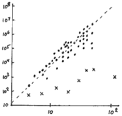
Figure 2. The number of characters needed to describe the fiducial vectors given in refs. [4] and [14] (dots), and the solutions given here (crosses). The dimension is given on the abscissa and the number of characters on the ordinate, in logarithmic scales. The dashed line is a ‘prediction’ by Magsino and Mixon [19], who plotted the dots.

The apparent complexity of the exact solutions for SICs has been noticeable from the start. Magsino and Mixon had the amusing idea to illustrate this by plotting the number of characters used to describe the coordinates of the fiducial vectors against the dimension [19]. By adding our solutions to their plot we see clearly that the description used here is very economical at least in this naive sense, see Figure 2. This is achieved by locating the fiducial vector in a subfield that is ‘complementary’ to the cyclotomic subfield of the ray class field. While our simplified solutions do not have the elegance achieved for the dimension ladder $d=5,15,195$ [20], the fact that we were able to manifest the behaviour under the Galois transformation $a\rightarrow-a$ (in all but one case) is some compensation.

The most striking feature seems to be the appearance of algebraic units among the components of the vectors (in all cases). Moreover our admittedly superficial analysis suggests that they are quite distinguished units. This observation may serve as a point of departure for further studies.

Acknowledgements: I thank Gary McConnell for help with (and patient explanations of) the number theory, Marcus Appleby for (indispensable) help with the calculations, and Markus Grassl for comments on the manuscript and for insights into dimension 67. I also thank the Mathematics Department at Stockholm University for allowing me to use their computer.

Appendix A Exact solutions

Here we give exact fiducial vectors for the SIC orbits 19e, 28c, 39i, 52d, and 124a. Exact fiducials for 4a, 7b, and 12b are given in the main text, see eqs. (15), (17), and (22). All our examples are available in exact form elsewhere, see Table 1 for references. Numbers denoted with the kernel letter $\eta$ are algebraic units. There are detailed comments on the solutions in the main text.

$$\psi_{19e}=N\left(\begin{array}[]{r}1\\ -x_{1}\\ x_{2}\\ x_{2}\\ -x_{1}\\ -x_{1}\\ -x_{1}\\ -x_{1}\\ x_{2}\\ -x_{1}\\ x_{2}\\ -x_{1}\\ x_{2}\\ x_{2}\\ x_{2}\\ x_{2}\\ -x_{1}\\ -x_{1}\\ x_{2}\end{array}\right)\hskip 28.45274pt\begin{array}[]{c}x_{1}=\frac{1}{10}a(m_{2}-1)\\ \\ x_{2}=\frac{1}{10}a(m_{2}+1)\\ \\ \\ \eta_{1}=\frac{x_{1}}{x_{2}}=\frac{1}{4}(a+5-m_{2}(a+1))\\ \\ \\ a=\sqrt{5}\\ \\ m_{2}=\sqrt{2a-1}\\ \\ \\ N=\sqrt{\frac{9a-5}{76}}\end{array}$$ (32)

$$\psi_{28c}=N\left(\begin{array}[]{c}0\\ 0\\ 0\\ 2\\ \hline\cr x_{3}\sigma^{6}\\ x_{4}\sigma\\ x_{5}\sigma^{7}\\ x_{1}\sigma^{4}\\ \hline\cr x_{5}\sigma^{6}\\ x_{3}\sigma^{5}\\ x_{4}\sigma^{3}\\ x_{1}\sigma^{4}\\ \hline\cr x_{6}\sigma^{2}\\ x_{7}\sigma^{5}\\ x_{8}\sigma^{3}\\ x_{2}\sigma^{4}\\ \hline\cr x_{4}\sigma^{2}\\ x_{5}\sigma^{5}\\ x_{3}\sigma^{7}\\ x_{1}\sigma^{4}\\ \hline\cr x_{7}\sigma^{6}\\ x_{8}\sigma\\ x_{6}\sigma^{3}\\ x_{2}\sigma^{4}\\ \hline\cr x_{8}\sigma^{2}\\ x_{6}\sigma\\ x_{7}\sigma^{7}\\ x_{2}\sigma^{4}\end{array}\right)\hskip 28.45274pt\begin{array}[]{c}x_{1}=\frac{1}{4}(a+5-2m_{2})\\ \\ x_{2}=\frac{1}{4}(a+5+2m_{2})\\ \\ x_{3}=\frac{b_{2}}{36}((-4c_{2}^{2}-(a-9)c_{2}+10b_{2})m_{2}\\ \hskip 8.53581pt+6c_{2}+3a-9)\\ \\ x_{3}x_{4}=\frac{1}{36}(((a+13)c_{2}^{2}+(a-1)c_{2}-a-37)m_{2}\\ +(a-1)c_{2}^{2}-2(2a+5)c_{2}-a+1)\\ \\ x_{3}x_{8}=\frac{1}{18}(-(a-1)c_{2}^{2}+2(2a+5)c_{2}+a-1)\\ \\ x_{4}x_{6}=\frac{1}{18}((a+13)c_{2}^{2}+(a-1)c_{2}-a-55)\\ \\ x_{3}x_{4}x_{5}=x_{6}x_{7}x_{8}=b_{2}\\ \\ \\ \eta_{1}=\frac{x_{7}}{x_{5}}\hskip 17.07164pt\eta_{2}=-\frac{x_{6}}{x_{4}}\hskip 17.07164pt\eta_{3}=-\frac{x_{8}}{x_{4}}\hskip 17.07164pt\eta_{4}=\frac{x_{7}}{x_{4}}\\ \\ \\ \sigma=e^{\frac{i\pi}{4}}\hskip 22.76219ptN=\sqrt{\frac{12a-58}{812}}\\ \\ \\ a=\sqrt{29}\hskip 28.45274ptb_{2}=\sqrt{a+6}\\ \\ 7c_{2}^{3}-42c_{2}+a-27=0\\ \\ m_{2}=\sqrt{\frac{a-1}{2}}\end{array}$$ (89)

$$\begin{array}[]{l}\psi_{39i}=N\left(\begin{array}[]{r}1\\ -x_{1}\\ x_{2}\\ \hline\cr-x_{3}\\ x_{7}\\ -x_{8}\\ \hline\cr x_{5}\\ -x_{9}\\ x_{10}\\ \hline\cr-x_{3}\\ x_{7}\\ -x_{8}\\ \hline\cr x_{4}\\ x_{11}\\ x_{12}\\ \hline\cr x_{5}\\ -x_{9}\\ x_{10}\\ \hline\cr x_{5}\\ -x_{9}\\ x_{10}\\ \hline\cr x_{6}\\ x_{13}\\ x_{14}\\ \hline\cr x_{6}\\ x_{13}\\ x_{14}\\ \hline\cr-x_{3}\\ x_{7}\\ -x_{8}\\ \hline\cr x_{4}\\ x_{11}\\ x_{12}\\ \hline\cr x_{6}\\ x_{13}\\ x_{14}\\ \hline\cr x_{4}\\ x_{11}\\ x_{12}\end{array}\right)\\ \\ \\ \\ \\ N=\sqrt{\frac{6(51a-150)-(23a-86)r_{1}}{780}}\\ \\ \\ \\ \\ \eta_{1}=\frac{x_{3}}{x_{1}}\\ \ \ \ \ \ \vdots\\ \\ \eta_{12}=\frac{x_{14}}{x_{1}}\end{array}\hskip 2.84526pt\begin{array}[]{c}x_{1}=-\frac{1}{520}(r1-10)b_{3}m_{2}-\frac{1}{120}(7a+25)r_{1}+\frac{1}{4}(a+3)\\ \\ x_{1}x_{2}=\frac{1}{60}(13a+40)r_{1}-\frac{1}{18}(11a+38)\\ \\ x_{3}=b_{4}\\ \\ x_{5}=\frac{1}{1520}(1430+650a+(-195-117a)r_{1}+b_{3}(-250-46a+(53+11a)r_{1})\\ +b_{4}(390-390a+(195+117a)r_{1}+b_{3}(210-30a+(-63+9a)r_{1})))\\ \\ x_{3}x_{4}=\frac{1}{2340}(((-22a-67)r_{1}+6(17a+50))b_{3}+130(a+1))\\ \\ x_{5}x_{6}=\frac{1}{2340}(((-22a-67)r_{1}+6(17a+50))b_{3}-130(a+1))\\ \\ x_{7}=\frac{1}{3120}(-2340-1170a+(650+299a)r_{1}+b_{3}(400+58a-(92+11a)r_{1})\\ +b_{4}(-390+390a+(195-273a)r_{1}+b_{3}(-390+78a+(63-9a)r_{1}))\\ +m_{2}(1560+390a+(-260-65a)r_{1}+b_{3}(-100-34a+(22+7a)r_{1})\\ +b_{4}(-390+(195+78a)r_{1}+b_{3}(-30+24a+(3-6a)r_{1}))))\\ \\ x_{9}=\frac{1}{3120}(-650-260a+b_{3}(150+12a-39r_{1})-195r_{1}\\ +b_{4}(-1170+390a-(195+39a)r_{1}+b_{3}(-330+114a+(69-21a)r_{1}))\\ +m_{2}(910+130a-(195+39a)r_{1}+b_{3}(-50-38a+(9+9a)r_{1})\\ +b_{4}(-390+195r_{1}+b_{3}(-30+36a+(3-6a)r_{1}))))\\ \\ x_{11}=\frac{1}{3120}(2080+910a+(-260-143a)r_{1}+b_{3}(-280+14a+(60-3a)r_{1})\\ +b_{4}(390-390a+(-195+273a)r_{1}+b_{3}(390-78a+(-63+9a)r_{1}))\\ +m_{2}(-1820-650a+(390+117a)r_{1}+b_{3}(60+30a-(10+7a)r_{1})\\ +b_{4}(390-(195+78a)r_{1}+b_{3}(30-24a+(-3+6a)r_{1}))))\\ \\ x_{13}=\frac{1}{3120}(-910-520a+(195+156a)r_{1}+b_{3}(30-60a+(-7+14a)r_{1})\\ +b_{4}(-1170+390a+(-195-39a)r_{1}+b_{3}(-330+114a+(69-21a)r_{1}))\\ +m_{2}(1170+390a+(-325-91a)r_{1}+b_{3}(-90-42a+(21+9a)r_{1})\\ +b_{4}(-390+195r_{1}+b_{3}(-30+36a+(3-6a)r_{1}))))\\ \\ x_{7}x_{8}=\frac{1}{4680}(-23790-7410a+(5395+1651a)r_{1}\\ +b_{3}(1850+590a-(421+133a)r_{1})\\ +b_{4}(10140+3120a+(-1950-546a)r_{1}\\ +b_{3}(-360-216a+(96+42a)r_{1})))\\ \\ x_{9}x_{10}=\frac{1}{4680}(-10010-2990a+(2015+611a)r_{1}\\ +b_{3}(690+258a-(147+57a)r_{1})\\ +b_{4}(1950+780a+(-975-156a)r_{1}\\ +b_{3}(-390-156a+(99+36a)r_{1})))\\ \\ x_{7}x_{8}x_{11}x_{12}=\frac{1}{21060}(226200+71760a-(50635+16003a)r_{1}\\ +b_{3}(-13090-4162a+(2928+930a)r_{1}))\\ \\ x_{9}x_{10}x_{13}x_{14}=\frac{1}{1/21060}(226200+71760a-(50635+16003a)r_{1}\\ +b_{3}(13090+4162a+(-2928-930a)r_{1}))\\ \\ \\ a=\sqrt{10}\hskip 14.22636ptr_{1}=\sqrt{20}\hskip 14.22636ptb_{3}=\sqrt{13(4a+15)(r_{1}+5)}\hskip 14.22636ptm_{2}=\sqrt{2a-1}\\ \\ b_{4}^{2}-\frac{1}{1560}(((6a-3)r_{1}-20a+10)b_{3}-13((8a+35)r_{1}-40a-130))b_{4}\\ +\frac{1}{2340}((22a+67)r_{1}-6(17a+50))b_{3}-\frac{1}{18}(a+1)=0\end{array}$$ (197)

$$\begin{array}[]{c}\psi_{52d}=N\left(\begin{array}[]{c}\sigma^{2}\\ \sigma\\ \sigma^{3}\\ m_{2}^{-1}\\ \hline\cr\eta_{1}\sigma^{2}\\ \eta_{2}\sigma\\ \eta_{3}\sigma^{7}\\ x_{1}\sigma^{4}\\ \hline\cr\eta_{4}\sigma^{2}\\ \eta_{5}\sigma^{5}\\ \eta_{6}\sigma^{3}\\ x_{2}\\ \hline\cr\eta_{2}\sigma^{2}\\ \eta_{3}\sigma^{5}\\ \eta_{1}\sigma^{3}\\ x_{1}\sigma^{4}\\ \hline\cr\eta_{7}\sigma^{6}\\ \eta_{8}\sigma\\ \eta_{9}\sigma^{7}\\ x_{3}\\ \hline\cr\eta_{6}\sigma^{2}\\ \eta_{4}\sigma^{1}\\ \eta_{5}\sigma^{7}\\ x_{2}\\ \hline\cr\eta_{5}\sigma^{6}\\ \eta_{6}\sigma\\ \eta_{4}\sigma^{3}\\ x_{2}\\ \hline\cr\eta_{10}\sigma^{2}\\ \eta_{11}\sigma\\ \eta_{12}\sigma^{3}\\ x_{4}\\ \hline\cr\eta_{11}\sigma^{2}\\ \eta_{12}\sigma\\ \eta_{10}\sigma^{3}\\ x_{4}\\ \hline\cr\eta_{3}\sigma^{6}\\ \eta_{1}\sigma\\ \eta_{2}\sigma^{3}\\ x_{1}\sigma^{4}\\ \hline\cr\eta_{9}\sigma^{6}\\ \eta_{7}\sigma^{5}\\ \eta_{8}\sigma^{3}\\ x_{3}\\ \hline\cr\eta_{12}\sigma^{2}\\ \eta_{10}\sigma\\ \eta_{11}\sigma^{3}\\ x_{4}\\ \hline\cr\eta_{8}\sigma^{2}\\ \eta_{9}\sigma^{5}\\ \eta_{7}\sigma^{7}\\ x_{3}\end{array}\right)\end{array}\hskip 5.69054pt\begin{array}[]{c}x_{1}=\frac{m_{2}}{8}((a+1)b_{2}-a-1)+\frac{1}{28}((a+2)b_{2}+2a-3)b_{4}\\ \\ x_{2}=\frac{m_{2}}{8}((a+1)b_{2}+a+1)-\frac{1}{28}((a+9)b_{2}+2a-10)b_{4}\\ \\ x_{1}x_{3}=\frac{1}{2}(7-a)+b_{2}\hskip 34.1433ptx_{2}x_{4}=\frac{1}{2}(a-7)+b_{2}\\ \\ \\ \eta_{1}=\frac{m_{2}b_{4}}{1820}(((22a-82)b_{2}-26(a-12))c_{2}^{2}-((46a-279)b_{2}+13(20a-149))c_{2}\\ +\frac{91}{2}((a+1)b_{2}+5a-47))-\frac{1}{520}(((6a+32)b_{2}-26a+104)c_{2}^{2}\\ +((8a+34)b_{2}-26a)c_{2}-(19a+97)b_{2}+13(11a-55))\\ \\ \eta_{2}=\frac{m_{2}b_{4}}{3640}((-(41a-583)b_{2}-13(23a-185))c_{2}^{2}+((87a+321)b_{2}+13(43a-243))c_{2}\\ +2(327a-1649)b_{2}+26(53a-363))-\frac{1}{520}(((2a+2)b_{2}+52)c_{2}^{2}\\ +((7a+85)b_{2}+13(3a-19))c_{2}+4(6a+45)b_{2}-52a-104)\\ \\ \eta_{1}\eta_{2}\eta_{3}=\frac{m_{2}b_{4}}{28}((19a-137)b_{2}+2(19a-137))+\frac{1}{8}((a-7)b_{2}-3a+21)\\ \\ \\ \eta_{4}=\frac{m_{2}b_{4}}{3640}((5(11a-41)b_{2}-13(19a-137))c_{2}^{2}-(10(2a-115)b_{2}+26(a-12))c_{2}\\ -10(11a-41)b_{2}+26(103a-781))+\frac{1}{520}(((2a+2)b_{2}-52)c_{2}^{2}\\ +((7a+85)b_{2}-13(3a-19))c_{2}+4(6a+45)b_{2}+52a+104)\\ \\ \eta_{5}=\frac{m_{2}b_{4}}{3640}(((2(53a-90)b_{2}-26(a-12))c_{2}^{2}+((79a+781)b_{2}-13(25a-209))c_{2}\\ -2(341a-1271)b_{2}-26(25a-209))+\frac{1}{520}(((8a+34)b_{2}+26(a-6))c_{2}^{2}\\ +((15a+119)b_{2}-13(a-19))c_{2}-(60a+242)b_{2}-26(6a-39))\\ \\ \eta_{4}\eta_{5}\eta_{6}=\frac{m_{2}b_{4}}{28}((-a+12)b_{2}+96a-697)-\frac{1}{8}((a-7)b_{2}+3a-21)\\ \\ \\ \eta_{8}\eta_{1}=-\frac{1}{260}(((a+79)b_{2}+13(3a-23))c_{2}^{2}\\ +((-3a+127)b_{2}+13(a-9))c_{2}-(a+391)b_{2}-13(3a-27))\\ \\ \eta_{9}\eta_{2}=\frac{1}{260}((-4a+48)b_{2}c_{2}^{2}\\ +((25a-27)b_{2}+65(-a+7))c_{2}+(30a+56)b_{2}+130(2a-15))\\ \\ \eta_{1}\eta_{2}\eta_{3}\eta_{7}\eta_{8}\eta_{9}=25a-182\\ \\ \\ \eta_{1}\eta_{8}\eta_{6}\eta_{11}=\frac{1}{10}((-17a+121)c_{2}^{2}-(11a-77)c_{2}+43a-301)\\ \\ \eta_{3}\eta_{7}\eta_{5}\eta_{10}=\frac{1}{10}((-20a+142)c_{2}^{2}+(19a-147)c_{2}+183a-1309)\\ \\ \eta_{4}\eta_{5}\eta_{6}\eta_{10}\eta_{11}\eta_{12}=25a-182\\ \\ \\ \sigma=e^{\frac{i\pi}{4}}\hskip 22.76219ptN=\frac{1}{2}\sqrt{\frac{53+a}{689}}\\ \\ \\ a=\sqrt{53}\hskip 22.76219ptb_{2}=\sqrt{15-2a}\hskip 22.76219ptb_{4}=\sqrt{\frac{13-(a+8)b_{2}}{2}}\\ \\ 2c_{2}^{3}+(3+a)c_{2}^{2}-(7-a)c_{2}-4a-6=0\\ \\ m_{2}=\frac{1}{13}\sqrt{34+5a}\end{array}$$ (304)

$$\psi_{124a}=N\left(\begin{array}[]{c}{\bf w}_{0}\\ {\bf u}_{1}\\ {\bf u}_{1}\\ {\bf v}_{1}\\ {\bf u}_{1}\\ {\bf u}_{2}\\ {\bf v}_{1}\\ {\bf u}_{3}\\ {\bf u}_{1}\\ {\bf u}_{2}\\ {\bf u}_{2}\\ {\bf v}_{2}\\ {\bf v}_{1}\\ {\bf v}_{2}\\ {\bf u}_{3}\\ {\bf v}_{3}\\ {\bf u}_{1}\\ {\bf v}_{1}\\ {\bf u}_{2}\\ {\bf u}_{3}\\ {\bf u}_{2}\\ {\bf v}_{2}\\ {\bf v}_{2}\\ {\bf v}_{3}\\ {\bf v}_{1}\\ {\bf u}_{3}\\ {\bf v}_{2}\\ {\bf v}_{3}\\ {\bf u}_{3}\\ {\bf v}_{3}\\ {\bf v}_{3}\\ \end{array}\right)\hskip 2.84526pt\begin{array}[]{c}\eta_{1}=\frac{1}{2}(3-a)m_{2}\\ \\ \eta_{2}=\frac{1}{4}((a-1)b_{2}-(a+1)m_{2})\hskip 22.76219pt2\eta_{2}\eta_{3}=3-a\\ \\ \eta_{4}=\frac{1}{124}((-(11a+27)c_{2}^{2}-(5a+1)c_{2}+10a+2)b_{2}m_{2}\\ +31(a+3)c_{2}^{2}+31(3a+1)c_{2})\\ \\ \eta_{5}=\frac{1}{124}(((38a+82)c_{2}^{2}+(37a+119)c_{2}+19a-83)b_{2}m_{2}\\ -62c_{2}-62(a-2))\\ \\ \eta_{7}=\frac{1}{124}(((38a+82)c_{2}^{2}+(37a+119)c_{2}+19a-83)b_{2}m_{2}\\ +62c_{2}+62(a-2))\\ \\ \eta_{9}=\frac{1}{124}(((11a+27)c_{2}^{2}+(5a+1)c_{2}-10a-2)b_{2}m_{2}\\ +31(a+3)c_{2}^{2}+31(3a+1)c_{2})\\ \\ \eta_{4}\eta_{5}\eta_{6}=\eta_{7}\eta_{8}\eta_{9}=a-2\\ \\ \\ \sigma=e^{\frac{i\pi}{4}}\hskip 28.45274ptN=\frac{1}{10}\sqrt{\frac{25+a}{31}}\\ \\ \\ a=\sqrt{5}\hskip 22.76219ptb_{2}=\sqrt{a+6}\hskip 22.76219ptm_{2}=\sqrt{\frac{a-1}{2}}\\ \\ 2c_{2}^{3}-(13-7a)c_{2}^{2}+(51-23a)c_{2}-18+8a=0\end{array}$$ (361)

$${\bf w}_{0}=\left[\begin{array}[]{l}2\\ 2\sigma^{7}\\ 2\sigma\\ 2\eta_{1}\end{array}\right]\hskip 11.38109pt{\bf u}_{1}=\left[\begin{array}[]{l}\eta_{4}\\ \eta_{5}\sigma^{7}\\ \eta_{6}\sigma^{5}\\ \eta_{2}\end{array}\right]\hskip 11.38109pt{\bf u}_{2}=\left[\begin{array}[]{l}\eta_{6}\sigma^{4}\\ \eta_{4}\sigma^{7}\\ \eta_{5}\sigma\\ \eta_{2}\end{array}\right]\hskip 11.38109pt{\bf u}_{3}=\left[\begin{array}[]{l}\eta_{5}\\ \eta_{6}\sigma^{3}\\ \eta_{4}\sigma\\ \eta_{2}\end{array}\right]$$ (378)

$${\bf v}_{1}=\left[\begin{array}[]{l}\eta_{7}\sigma^{4}\\ \eta_{8}\sigma^{7}\\ \eta_{9}\sigma\\ \eta_{3}\sigma^{4}\end{array}\right]\hskip 25.60747pt{\bf v}_{2}=\left[\begin{array}[]{l}\eta_{8}\\ \eta_{9}\sigma^{7}\\ \eta_{7}\sigma^{5}\\ \eta_{3}\sigma^{4}\end{array}\right]\hskip 25.60747pt{\bf v}_{3}=\left[\begin{array}[]{l}\eta_{9}\\ \eta_{7}\sigma^{3}\\ \eta_{8}\sigma\\ \eta_{3}\sigma^{4}\end{array}\right]\hskip 22.76219pt$$ (391)

References

• [1] G. Zauner: Quantendesigns. Grundzรผge einer nichtkommutativen Designtheorie, PhD thesis, Universitรคt Wien, 1999; also published as Quantum designs: Foundations of a noncommutative design theory, Int. J. Quant. Inf. 9 (2011) 445.
• [2] J. M. Renes, R. Blume-Kohout, A. J. Scott, and C. M. Caves, Symmetric informationally complete quantum measurements, J. Math. Phys. 45 (2004) 2171.
• [3] C. A. Fuchs, M. C. Hoan, and B. C. Stacey, The SIC question: History and state of play, Axioms 6 (2017) 21.
• [4] A. J. Scott and M. Grassl, SIC-POVMs: A new computer study, J. Math. Phys. 51 (2010) 042203.
• [5] A. J. Scott, SICs: Extending the list of solutions, arXiv:1703.03993.
• [6] M. Appleby, S. Flammia, G. McConnell, and J. Yard, Generating ray class fields of real quadratic fields via complex equiangular lines, arXiv:1604.06098, to appear in Acta Arithmetica.
• [7] D. M. Appleby, SIC-POVMs and the extended Clifford group, J. Math. Phys. 46 (2005) 052107.
• [8] M. Grassl, Computing equiangular lines in complex space, Lecture Notes in Computer Science 5393 (2008) 89.
• [9] G. S. Kopp, SIC-POVMs and the Stark conjectures, Int. Math. Res. Not. IMRN., published online doi.org/10.1093/imrn/rnz153 (2019).
• [10] D. M. Appleby, H. Yadsan-Appleby, and G. Zauner, Galois automorphisms of symmetric measurements, Quantum Inf. Comp. 13 (2013) 672.
• [11] D. Hilbert, Mathematical problems, Bull. AMS 8 (1902) 437.
• [12] G. H. Hardy and E. M. Wright: An Introduction to the Theory of Numbers, 4th ed., Oxford U. P. 1960.
• [13] D. M. Appleby, I. Bengtsson, S. Brierley, ร…. Ericsson, M. Grassl, and J.-ร…. Larsson, Systems of imprimitivity for the Clifford group, Quantum Inf. Comp. 14 (2014) 0339; also available with six additional pages as arXiv:1210.1055.
• [14] M. Appleby, T.-Y. Chien, S. Flammia, and S. Waldron, Constructing exact symmetric informationally complete measurements from numerical solutions, J. Phys. A51 (2018) 165302.
• [15] M. Grassl and A. J. Scott, Fibonacciโ€“Lucas SIC-POVMs, J. Math. Phys. 58 (2017) 122201.
• [16] Markus Grassl, unpublished.
• [17] K. Dixon and S. Salamon, Moment maps and Galois orbits for SIC-POVMs, arXiv:1912.03209.
• [18] D.ย M.ย Appleby, I.ย Bengtsson, S.ย Brierley, M.ย Grassl, D.ย Gross, and J.-ร….ย Larsson, The monomial representations of the Clifford group, Quantum Inf.ย Comp. 12 (2012) 0404.
• [19] M. Magsino and D. G. Mixon, Biangular Gabor frames and Zaunerโ€™s conjecture, arXiv:1908.02801.
• [20] M. Appleby and I. Bengtsson, Simplified exact SICs, J. Math. Phys. 60 (2019) 062203.