Internet congestion control: from stochastic to dynamical models

Abstract

Since its inception, control of data congestion on the Internet has been based on stochastic models. One of the first such models was Random Early Detection. Later, this model was reformulated as a dynamical system, with the average queue sizes at a router’s buffer being the states. Recently, the dynamical model has been generalized to improve global stability. In this paper we review the original stochastic model and both nonlinear models of Random Early Detection with a two-fold objective: (i) illustrate how a random model can be “smoothed out” to a deterministic one through data aggregation, and (ii) how this translation can shed light into complex processes such as the Internet data traffic. Furthermore, this paper contains new materials concerning the occurrence of chaos, bifurcation diagrams, Lyapunov exponents and global stability robustness with respect to control parameters. The results reviewed and reported here are expected to help design an active queue management algorithm in real conditions, that is, when system parameters such as the number of users and the round-trip time of the data packets change over time. The topic also illustrates the much-needed synergy of a theoretical approach, practical intuition and numerical simulations in engineering.

This paper is dedicated to Manfred Denker on the occasion of his 75th birthday

Keywords Internet congestion control  $\cdot$ Adaptive queue management  $\cdot$ Random early detection  $\cdot$ Discrete-time dynamical systems  $\cdot$ Global stability  $\cdot$ Robust setting of control parameters

AMS Subject Classification: 37E05, 39A50, 37G35, 37N35

1 Introduction

Internet Protocols (IP) networks include memory buffers to manage the network traffic by implementing a queue algorithm into buffers. Obviously, the length of this queue is upper bounded by the size of the buffer, and they are not effective in their purpose of managing bursts of packets if they run at full capacity. Therefore, in a scenario of congestion some actions have to be taken to avoid overflow or a system collapse. An Active Queue Management (AQM) is an algorithm acting on the queue to control its length and, thus, achieve an efficient control of the system congestion. Such management also enables the transmission control protocols (TCPs) to share links properly.

The Random Early Detection (RED) algorithm [12] was the first formal and complete AQM system implemented in TCP/IP networks [2]. One of the purposes of designing the RED queue management algorithm was to detect the beginning of traffic congestion well in advance. This would allow the system to act in two ways: starting to gradually discard packets and reducing the transmission rate to that node, both actions aimed at avoiding scenarios of massive packet discarding, system collapse or overflow.

The congestion detection indicator used by the RED queue management is an Exponentially Weighted Moving Average (EWMA) of the queue length. EWMA actually acts as a low-pass filter that smooths the instantaneous queue length bursts. The degree of smoothing is determined by a weight $w$. The algorithm uses a decision mechanism based on a linear probability distribution to determine when packets are rejected. When a packet reaches the queue, the algorithm proceeds as follows. If the weighted average of the queue length is less than a minimum threshold $q_{\min}$, no action is taken and the packet simply remains in the queue. An average queue length between $q_{\min}$ and another higher threshold $q_{\max}$ is interpreted as congestion, in which case an early drop command is executed. More specifically, the RED algorithm drops an incoming packet with a probability that depends on the EWMA. This means that adequate $q_{\min}$ and $q_{\max}$ values are a requirement for good performance. Finally, if the average queue length is greater than the maximum threshold $q_{\max}$, then it is understood that the congestion is persistent, and packets are dropped to avoid a lasting full queue. In this case, the packets are dropped with probability 1.

RED has been the most studied AQM to date, and has been the basis for the development of new AQM systems. This is so not only because it was the first one developed in the Internet community, but also because of several drawbacks that this algorithm entails, some of which have not yet been successfully resolved. In particular, it is difficult to adjust the RED parameters for adequate performance due to their high sensitivity. Moreover, even if the RED parameters are adjusted properly, they are also very sensitive to the network conditions. Thus, a set of parameters can work perfectly for a given load of data traffic but not be suitable if the load varies slightly. Obviously, this is not a desirable feature since Internet traffic conditions change rapidly. This is, by far, what has most affected a widespread implementation of RED. There are many proposals in the literature to overcome these difficulties via modifications of the RED algorithm, e.g., [4, 5, 6, 13, 8, 7].

Numerical experiments and simulations have usually been the main tool for setting parameters, also in the papers cited above. As a result, many of the conclusions published in the literature are based only on numerical results, thus lacking the necessary mathematical rigor to support them. The first theoretical study of RED we are aware of was done by Ranjan et al. [19]. This was possible because these authors reformulated the original, stochastic RED model as a discrete-time dynamical model, thus allowing them to apply the powerful methods of nonlinear dynamics. In particular, the authors showed that their dynamical RED model was chaotic. This first dynamical model was generalized in [9, 10, 3] with the objective of enhancing the controllability of the model. To this end, two new control parameters where introduced via the probability law for dropping incoming packets. Moreover, the analysis of the generalized model in [3] focused on global stability rather than local stability like in [19]. Numerical results (e.g., bifurcation diagrams and parametric domains of robustness) suggest that, as expected, the generalized model is more stable than the original one. This is a welcome feature for the prospective design of an AQM in real conditions, that is, when system parameters such as the number of users and the round-trip time change over time.

In this paper we review the original RED dynamical model [19] and the main results of the generalized dynamical model [3] with a two-fold objective: (i) illustrate how a random model can be “smoothed out” to a deterministic one through data aggregation (sometimes with much ingenuity), and (ii) how this translation can provide useful insights into complex processes such as data traffic on the Internet. Furthermore, this paper contains new materials concerning the occurrence of chaos, bifurcation diagrams, Lyapunov exponents and global stability robustness with respect to control parameters, as we detail in short. The topic (Internet congestion control) illustrates also the much-needed synergy of a theoretical approach, practical intuition and numerical simulations in engineering.

The rest of this paper is organized as follows. In Section 2 we present the probabilistic RED algorithm and how to derive a nonlinear model by trading off detailed information (queue size) for coarse-grained information (average queue length). Our presentation is based on [19]. In Section 3, we follow [3] to generalize the said nonlinear model with the purpose of increasing the number of control parameters and thus the control leverage. We have also added in Section 3 the proof that the generalized RED dynamics can be chaotic (depending on the parameters) in the sense of Li-Yorke. The main results in [3] concerning the global stability of the unique fixed point of the RED dynamic are summarized in Section 4, while Section 5 recaps a few more particular results with a potential to be implemented in real congestion control. The graphics and numerical simulations presented in Section 6, all of them new, deal principally with bifurcation diagrams and Lyapunov exponents (Section 6.1), as well as with the robustness of the fixed point with respect to the new control parameters (Section 6.2). Section 7 contains the concluding remarks and an outlook.

2 Random Early Detection

We follow [19] for the description of RED and the derivation of its discrete-time dynamical model. Our main concern is the mathematical content of the model, hence technical details will be kept to a minimum.

Consider the following communication network throughout. $N$ users (i.e., $N$ uniform TCP connections) are connected to a Router 1 which shares an Internet link (bottleneck link) with Router 2. The capacity of this channel (i.e., the maximum amount of error-free information that can be transmitted over the channel per unit time) is $C$. Further parameters of the system are the packet size $M$, the round-trip time (propagation delay with no queuing delay) $d$ of the packets, and the buffer size $B$ of Router 1. So, $B$ is the maximum number of packets that the buffer of Router 1 can store. The queue length or size $q$ at the buffer at a given time is the number of packets in the buffer at that time, so $q=0,1,...,B$.

In the RED model, the probability $p$ of dropping an incoming packet at a router depends on the ‘average’ queue length $q^{\mathtt{ave}}$ (to be defined below) as follows:

$$p(q^{\mathtt{ave}})=\left\{\begin{array}[]{cl}0&\text{if }q^{\mathtt{ave}}<q_{\min},\\ 1&\text{if }q^{\mathtt{ave}}>q_{\max},\\ \frac{q^{\mathtt{ave}}-q_{\min}}{q_{\max}-q_{\min}}p_{\max}&\text{otherwise.}\end{array}\right.$$ (1)

Thus, $q_{\min}$ and $q_{\max}$ are the lower and upper thresholds of $q^{\mathtt{ave}}$ for accepting and dropping an incoming packet, respectively, and $p_{\max}$ is the selected drop probability when $q^{\mathtt{ave}}=q_{\max}$, i.e., the maximum packet drop probability. The average queue length is updated at the time of a packet arrival according to the averaging

$$q_{\mathtt{new}}^{\mathtt{ave}}=(1-w)q_{\mathtt{old}}^{\mathtt{ave}}+wq^{\mathtt{cur}}$$ (2)

between the previous average queue length $q_{\mathtt{old}}^{\mathtt{ave}}$ and the current queue length $q^{\mathtt{cur}}$, where $0<w<1$ is the averaging weight. The initial average queue length is set in an unspecified way; from then on, the average queue length is defined by the rule (2). The higher $w$, the faster the RED mechanism reacts to the actual buffer occupancy. In practice $w$ is taken rather small, typically $\lesssim 0.2$ [21].

On the way to a discrete-time nonlinear dynamical model, let $q_{n}^{\mathtt{ave}}$ be the average queue length at time $n=1,2,...$ Then, the packet drop probability at time $n$, $p_{n}$, determines the queue length at time $n+1$, $q_{n+1}$. In turn, $q_{n+1}$ is used to compute $q_{n+1}^{\mathtt{ave}}$ according to the averaging rule (2). Finally, $q_{n+1}^{\mathtt{ave}}$ determines the drop probability at time $n+1$, $p_{n+1}$, via Equation (1). In sum, the update of $p_{n}$ has this formal structure:

$$\left\{\begin{array}[]{l}q_{n+1}=G(p_{n})\\ q_{n+1}^{\mathtt{ave}}=(1-w)q_{n}^{\mathtt{ave}}+wq_{n+1}\\ p_{n+1}=H(q_{n+1}^{\mathtt{ave}})\end{array}\right.$$ (3)

where $H(q_{n+1}^{\mathtt{ave}})=p(q_{n+1}^{\mathtt{ave}})$ is given in (1). From (3) it follows

$$q_{n+1}^{\mathtt{ave}}=(1-w)q_{n}^{\mathtt{ave}}+wG(H(q_{n}^{\mathtt{ave}})).$$ (4)

So this equation will define a dynamic model for the average queue length once the function $G$ is determined.

It was shown in [14, 16, 17, 18] that, if the packet size $M$, the time delay $d$ and the packet loss probability $p$ are known, the stationary throughput of a typical TCP connection can be approximated by

$$T(p,d)=\frac{MK}{\sqrt{p}d}+o\left(\frac{1}{\sqrt{p}}\right),$$ (5)

where $K$ is a constant usually set equal to $\sqrt{3/2}$. Therefore, the steady-state packet drop probability $p_{r}$ such that the aggregate throughput of connections equals the link capacity, is given by

$$N\frac{MK}{\sqrt{p_{r}}d}=C.$$ (6)

This is the smallest drop probability such that $p_{n}\geq p_{r}$ entails $q_{n+1}=0$. By (6),

$$p_{r}=\left(\frac{NMK}{Cd}\right)^{2}.$$ (7)

The corresponding average queue length $q_{r}^{\mathtt{ave}}$ such that $q_{n}^{\mathtt{ave}}>q_{r}^{\mathtt{ave}}$ implies $q_{n+1}=0$, follows from (1):

$$q_{r}^{\mathtt{ave}}=\left\{\begin{array}[]{ll}\frac{q_{\max}-q_{\min}}{p_{\max}}p_{r}+q_{\min}&\text{if }p_{r}\leq p_{\max},\\ q_{\max}&\text{otherwise.}\end{array}\right.$$ (8)

Note that

$$q_{r}^{\mathtt{ave}}\leq q_{\max}\text{.}$$ (9)

Otherwise, if $p_{n}<p_{r}$ (i.e., $q_{n+1}>0$) and $q_{n+1}\leq B$, the Internet link capacity between Routers 1 and 2 is fully utilized and the round-trip time of a packet arriving at time $n+1$ is augmented from $d$ (no queuing delay) to $d+Mq_{n+1}/C$. From (see (6))

$$N\frac{MK}{\sqrt{p_{n}}(d+\frac{Mq_{n+1}}{C})}=C,$$ (10)

we obtain

$$q_{n+1}=\frac{C}{M}\left(\frac{NKM}{\sqrt{p_{n}}C}-d\right).$$ (11)

Since $q_{n+1}$ is a strictly decreasing function of $p_{n}$, there exists $\min\{p_{n},\,n\geq 1:q_{n+1}=B\}=:p_{l}$, where

$$p_{l}=\left(\frac{NMK}{BM+Cd}\right)^{2}$$ (12)

by (11). The corresponding average queue length is

$$q_{l}^{\mathtt{ave}}=\frac{q_{\max}-q_{\min}}{p_{\max}}p_{l}+q_{\min}=\frac{q_{\max}-q_{\min}}{p_{\max}}\left(\frac{NMK}{BM+Cd}\right)^{2}+q_{\min}.$$ (13)

Therefore, $q_{n+1}=B$ for $p_{n}\leq p_{l}$, i.e., $q_{n}^{\mathtt{ave}}\leq q_{l}^{\mathtt{ave}}$. Note that

$$q_{l}^{\mathtt{ave}}>q_{\min}\text{.}$$ (14)

Comparison of (13) with (8) shows that

$$q_{l}^{\mathtt{ave}}<q_{r}^{\mathtt{ave}}$$ (15)

if $p_{r}<p_{\max}$. For $q_{l}^{\mathtt{ave}}<q_{r}^{\mathtt{ave}}$ to hold also when $p_{r}\geq p_{\max}$ (i.e., $q_{r}^{\mathtt{ave}}=q_{\max}$), it is necessary that

$$\left(\frac{NMK}{BM+Cd}\right)^{2}<p_{\max}.$$ (16)

From Equations (11) and the definition of $p_{r}$, Equation (7), and $p_{l}$, Equation (13), it follows that the function $G$ in (3) is defined as

$$q_{n+1}=G(p_{n})=\begin{cases}B&\text{if }p_{n}\leq p_{l},\\ \frac{NK}{\sqrt{p_{n}}}-\frac{Cd}{M}&\text{if }p_{l}<p_{n}<p_{r},\\ 0&\text{if }p_{n}\geq p_{r}.\end{cases}$$ (17)

Finally, plugging (17) into (4) we conclude that the time evolution of the average queue length is given by the nonlinear dynamic

$$q_{n+1}^{\mathtt{ave}}=\begin{cases}(1-w)q_{n}^{\mathtt{ave}}+wB&\text{if }q_{n}^{\mathtt{ave}}\leq q_{l}^{\mathtt{ave}},\\ (1-w)q_{n}^{\mathtt{ave}}+w\left(\frac{NK}{\sqrt{p_{n}}}-\frac{Cd}{M}\right)&\text{if }q_{l}^{\mathtt{ave}}<q_{n}^{\mathtt{ave}}<q_{r}^{\mathtt{ave}},\\ (1-w)q_{n}^{\mathtt{ave}}&\text{if }q_{n}^{\mathtt{ave}}\geq q_{r}^{\mathtt{ave}},\end{cases}$$ (18)

where, see (1),

$$p_{n}=p(q_{n}^{\mathtt{ave}})=\frac{q_{n}^{\mathtt{ave}}-q_{\min}}{q_{\max}-q_{\min}}p_{\max}$$ (19)

since $q_{l}^{\mathtt{ave}}>q_{\min}$ by (14) and $q_{r}^{\mathtt{ave}}\leq q_{\max}$ by (9).

The mapping $q_{n}^{\mathtt{ave}}\mapsto q_{n+1}^{\mathtt{ave}}$ of the interval $[0,B]$, Equation (18), is affine on $[0,q_{l}^{\mathtt{ave}}]$, $\cup$-convex on $[q_{l}^{\mathtt{ave}},q_{r}^{\mathtt{ave}}]$ and linear on $[q_{r}^{\mathtt{ave}},B]$, where $[q_{l}^{\mathtt{ave}},q_{r}^{\mathtt{ave}}]$ can be shown to be a trapping interval of the ensuing dynamic. It is, therefore, not surprising that this dynamic may be chaotic, depending on the parameter settings [19]. This is bad news for the sake of a stable control of the Internet data traffic, which is our main concern. The RED dynamical model (18) has 5 system parameters ($N,C,d,M,B$) and 4 user parameters ($p_{\max},q_{\min},q_{\max},w$). The former are constrained by condition (16). The latter are also called control parameters because they can be tuned at will to stabilize the dynamic if necessary. Among the system parameters, the most critical ones are $N$ and $d$ because they may change in real time. When it comes to the implementation of adaptive control, the averaging weight $w$ is the most practical choice. In the next section we will add to $w$ two more control parameters to improve the stability properties of the RED dynamical model (18).

3 A generalized RED dynamical model

For a more compact notation, we introduce normalized state variables and thresholds,

$$x_{n}=\frac{q_{n}^{\mathtt{ave}}}{B},\;x_{\min}=\frac{q_{\min}}{B},\;x_{\max}=\frac{q_{\max}}{B},$$ (20)

as well as the dimensionless constants

$$A_{1}=\frac{NK}{\sqrt{p_{\max}}B},\;\;A_{2}=\frac{Cd}{MB}.$$ (21)

Actually, out of the parameters in (21) only $C$, $d$ and $M$ are dimensional (given, say, in kilobytes per second, seconds and kilobytes, respectively); the other parameters are pure numbers. The constant $K$ will be set equal to $\sqrt{3/2}$ for definiteness, see (5). According to Equation (16), $A_{1}$ and $A_{1}$ are related as follows.

Proposition 1

The constants $A_{1}$ and $A_{2}$ of the RED model (18) are subject to the constraint

$$A_{1}<A_{2}+1.$$ (22)

Inequality (22) is assumed throughout this paper. Since $p_{\max}$ appears in the denominator of $A_{1}$, the larger $p_{\max}$, the better for the constraint (22) to be fulfilled.

On the grounds explained in Sections 1 and 2, the RED dynamical model (18) was generalized in [3] by replacing the probability law (19) by

$$p(x_{n})=I_{\alpha,\beta}(z(x_{n}))\cdot p_{\max},$$ (23)

where $I_{\alpha,\beta}(z)$, $0\leq z\leq 1$, is the beta distribution function (or normalized incomplete beta function),

$$I_{\alpha,\beta}(z)=\frac{\mathfrak{B}(z;\alpha,\beta)}{\mathfrak{B}(1;\alpha,\beta)},\;\;\;\;\mathfrak{B}(z;\alpha,\beta)=\int_{0}^{z}t^{\alpha-1}(1-t)^{\beta-1}dt,$$ (24)

with $\alpha,\beta>0$, and

$$z(x_{n})=\frac{x_{n}-x_{\min}}{x_{\max}-x_{\min}},\;\;x_{\min}\leq x_{n}\leq x_{\max}.$$ (25)

Since $I_{1,1}(z)=z$, we recover the conventional RED model (18) for $\alpha=\beta=1$. The beta distribution is related to the chi-square distribution [1]. By definition, $I_{\alpha,\beta}(z)$ is strictly increasing, hence invertible. Its inverse, $I_{\alpha,\beta}^{-1}(z)$, is also strictly increasing.

The packet dropping probability $p(x_{n})$ is plotted in Figure 1 for different values of the control parameters $\alpha$, $\beta$ and $p_{\max}$. The left panel ($\alpha=\beta=1$) corresponds to (19) with $p_{\max}=0.5$.

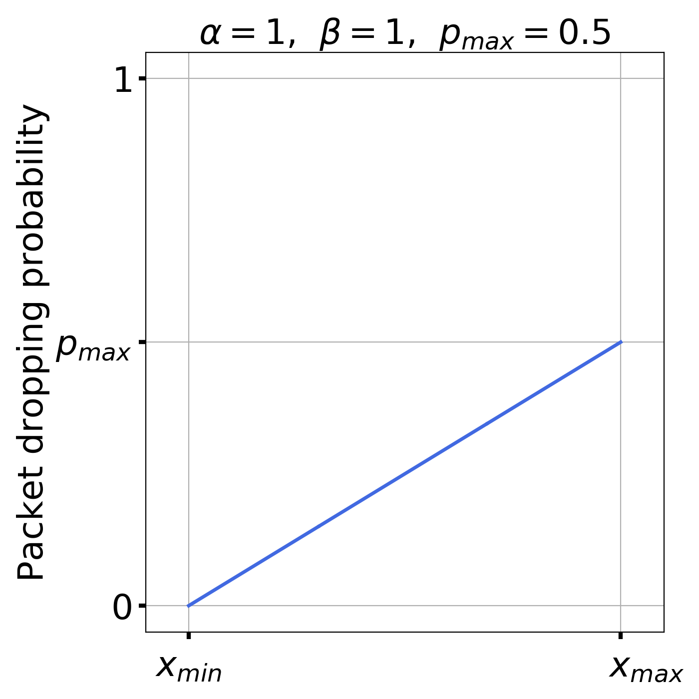
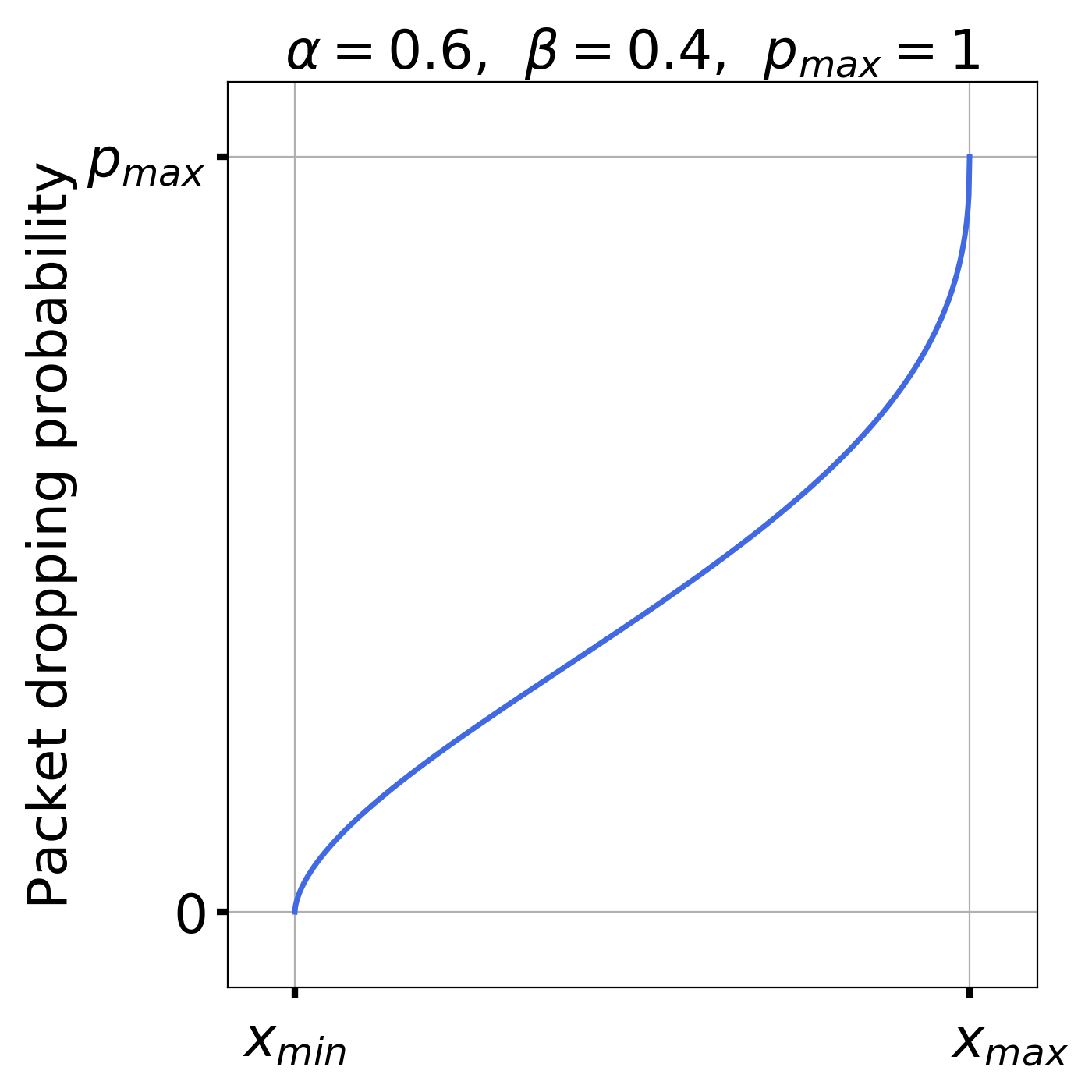
Figure 1: Packet dropping probability, Equations (23)-(25), for the settings of the control parameters $\alpha,\beta$ and $p_{\max}$ displayed at the top of the panels.

Thus, we consider hereafter a dynamical system,

$$x_{n+1}=f(x_{n}),$$ (26)

where the mapping $f:[0,1]\rightarrow[0,1]$ is defined as

$$f(x)=\left\{\begin{array}[]{ll}(1-w)x+w&\text{if }0\leq x\leq\theta_{l},\\ (1-w)x+w\left(\frac{A_{1}}{\sqrt{I_{\alpha,\beta}(z(x))}}-A_{2}\right)&\text{if }\theta_{l}<x<\theta_{r},\\ (1-w)x&\text{if }\theta_{r}\leq x\leq 1,\end{array}\right.$$ (27)

and the thresholds $\theta_{l}$, $\theta_{r}$ are given by

$$\theta_{l}=(x_{\max}-x_{\min})I_{\alpha,\beta}^{-1}\left(z_{1}\right)+x_{\min},\text{\ \ }\;z_{1}=\left(\frac{A_{1}}{A_{2}+1}\right)^{2},$$ (28)

($z_{1}<1$ by (16)) and

$$\theta_{r}=\left\{\begin{array}[]{ll}(x_{\max}-x_{\min})I_{\alpha,\beta}^{-1}(z_{2})+x_{\min}&\text{if }z_{2}=\left(\frac{A_{1}}{A_{2}}\right)^{2}\leq 1,\\ x_{\max}&\text{otherwise.}\end{array}\right.$$ (29)

Hence, $\theta_{l}>x_{\min}$,

$$\left\{\begin{array}[]{ll}\theta_{r}<x_{\max}&\text{if }0<A_{1}<A_{2},\\ \theta_{r}=x_{\max}&\text{if }A_{2}\leq A_{1}<A_{2}+1,\end{array}\right.$$ (30)

and $\theta_{l}<\theta_{r}$ by (22).

The thresholds $\theta_{l}$ and $\theta_{r}$ are set so that $f$ is continuous on $[0,1]$, except when $A_{1}>A_{2}$, in which case $f$ is lower semicontinuous at $\theta_{r}$. Indeed, if $A_{1}>A_{2}$,

$$f(\theta_{r}-) = f(x_{\max}-)=\lim_{x\rightarrow x_{\max}-}f(x)=(1-w)x_{\max}+w(A_{1}-A_{2})$$ (31)

$$= f(x_{\max})+w(A_{1}-A_{2})>f(x_{\max})=f(\theta_{r}),$$

where we used $I_{\alpha,\beta}(z(x_{\max}))=I_{\alpha,\beta}(1)=1$, on the second line.

We will numerically show in Section 6 that the additional control parameters $\alpha$ and $\beta$ of the generalized RED nonlinear model (27) do improve the stability of the dynamic. This is important to enable controllability also in a real environment, where the system parameters may change over time. It is worth noting that $p_{\max}$ and all 5 system parameters go into the dynamic through the constants $A_{1}$ and $A_{2}$, which amounts to a high degeneracy of the dynamic with respect to the system parameters. Note also that $A_{1}$, $A_{2}$ and the control parameters except $w$ go into the thresholds $\theta_{l}$ and $\theta_{r}$ as well.

We show next that the dynamical system defined by (27) can be chaotic, depending of the parameter setting. To be more specific, we are going to prove analytically that the dynamic $x_{n+1}=f(x_{n})$ may exhibit chaos in the sense of Li-Yorke [15]. Numerical evidence in the form of bifurcation diagrams and Lyapunov exponents will be presented in Section 6.

We recall the main result of [15] first.

Theorem 2

Let $J$ be a closed interval and $F:J\rightarrow J$ a continuous mapping. Suppose that there is $x_{0}\in J$ such that

$$F^{3}(x_{0})\leq x_{0}<F(x_{0})<F^{2}(x_{0})$$ (32)

or

$$F^{3}(x_{0})\geq x_{0}>F(x_{0})>F^{2}(x_{0}).$$ (33)

Then

(1)

for every $k\in N$ there is a periodic point in $J$ with period $k$;

(2)

there is an uncountable set $S\subset J$ containing no periodic points, which satisfies the following conditions:

(i)

For every $x,y\in S$, $x\neq y$,

$$\underset{n\rightarrow\infty}{\lim\sup}\left|F^{n}(x)-F^{n}(y)\right|>0$$

and

$$\underset{n\rightarrow\infty}{\lim\inf}\left|F^{n}(x)-F^{n}(y)\right|=0.$$

(ii)

For every $x\in S$ and periodic point $p\in J,$

$$\underset{n\rightarrow\infty}{\lim\sup}\left|F^{n}(x)-F^{n}(p)\right|=0.$$

In our case, $J=[0,1]$ and $F=f$, Equation (27). For $f$ to be continuous, we assume $A_{1}\leq A_{2}$ for the time being. Following [19], we choose $x_{0}=\theta_{r}/(1-w)$ with $w<1-\theta_{r}$ (so that $\theta_{r}<x_{0}<1$). Therefore,

$$f(x_{0})=f\left(\frac{\theta_{r}}{1-w}\right)=\theta_{r},$$

and

$$f^{2}(x_{0})=f\left(\theta_{r}\right)=(1-w)\theta_{r},$$

hence

$$x_{0}>f(x_{0})>f^{2}(x_{0}).$$

By (33) we only need that $f^{3}(x_{0})\geq x_{0}$ to conclude the presence of chaos in the form stated in the points (1) and (2) of Theorem 2. There are two cases: $f^{2}(x_{0})>\theta_{l}$, i.e., $w<(\theta_{r}-\theta_{l})/\theta_{r}$ (Case I) and $f^{2}(x_{0})\leq\theta_{l}$, i.e., $w\geq(\theta_{r}-\theta_{l})/\theta_{r}$ (Case II).

In Case I, $\theta_{l}<f^{2}(x_{0})<\theta_{r}$, hence $f^{3}(x_{0})=f(f^{2}(x_{0}))\geq x_{0}$ if and only if

$$f\left((1-w)\theta_{r}\right)=(1-w)^{2}\theta_{r}+w\left(\frac{A_{1}}{\sqrt{I_{\alpha,\beta}(z((1-w)\theta_{r})}}-A_{2}\right)\geq\frac{\theta_{r}}{1-w},$$ (34)

where $z((1-w)\theta_{r})=((1-w)\theta_{r}-x_{\min})/(x_{\max}-x_{\min})$. To verify that inequality (34) can be satisfied, use the following lower bound of the lhs of (34):

$$f\left((1-w)\theta_{r}\right) \geq (1-w)^{2}\theta_{r}+\frac{wA_{1}}{\sqrt{I_{\alpha,\beta}(z((1-w)\theta_{r})}}$$ (35)

$$\geq (1-w)^{2}\theta_{r}+\frac{wA_{1}}{\sqrt{I_{\alpha,\beta}(z(\theta_{r})}},$$

since $I_{\alpha,\beta}(z)^{-1/2}$ is a monotone decreasing function. Set now $w=\epsilon\ll 1$. Then, a sufficient condition for (34) to hold is that the lower bound (35) is greater than $\frac{\theta_{r}}{1-\epsilon}$, that is,

$$(1-2\epsilon)\theta_{r}+\frac{\epsilon A_{1}}{\sqrt{I_{\alpha,\beta}(z(\theta_{r})}}\geq(1+\epsilon)\theta_{r}$$

to first order in $\epsilon$. It follows that

$$\theta_{r}\sqrt{I_{\alpha,\beta}(z(\theta_{r})}\leq\frac{A_{1}}{3}$$ (36)

suffices for $f^{3}(x_{0})\geq x_{0}$ to hold, provided $w$ is sufficiently small.

In Case II, $f^{2}(x_{0})\leq\theta_{l}$, hence $f^{3}(x_{0})=f(f^{2}(x_{0}))\geq x_{0}$ if and only if

$$f\left((1-w)\theta_{r}\right)=(1-w)^{2}\theta_{r}+w\geq\frac{\theta_{r}}{1-w},$$

hence

$$\theta_{r}\leq\frac{1-w}{3-w+w^{2}}<\frac{1}{3}.$$ (37)

In sum, compliance with (34) if $w<(\theta_{r}-\theta_{l})/\theta_{r}$, or with (37) otherwise, implies chaos in the sense of Theorem 2. Unlike condition (34), which involves all the parameters of the model, condition (37) only involves the control parameter $w$. Actually, we expect the condition (36) to be the general criterion because, as mentioned in Section 2, typically $w\lesssim 0.2$. Needless to say, the possibility of a chaotic behavior poses a challenge to the control design.

4 Global stability of the generalized RED model: main results

In this paper we are interested in a stable and robust congestion control of the Internet data traffic based on the generalized RED model. This means that the system remains on, or evolves within the basin of attraction of, a fixed point for suitably chosen control parameters, also when the system parameters (grouped in the constants $A_{1}$ and $A_{2}$) and the control parameters (mainly $w$, $\alpha$ and $\beta$) change slightly. This way one can expect to keep the system in a neighborhood of the fixed point when both system parameters and (consequently) control parameters change in real time. Recall that $A_{1}<A_{2}+1$ (Proposition 1).

To this end, this section summarizes the most important results on global stability of the dynamical system (27). Proofs and additional detail can be found in [3]. The study of robustness with respect to the control parameters $\alpha$, $\beta$ and $w$ is deferred to Section 6.2.

Theorem 3

The mapping $f$ has a unique fixed point $x^{\ast}\in(\theta_{l},\theta_{r})$ if and only if $A_{1}<A_{2}+x_{\max}$; otherwise, it has none. Furthermore, $x^{\ast}$ does not depend on $w$.

To compute the fixed point $x^{\ast}$ one has in general to solve numerically the equation $f(x)=x$ (with $\theta_{l}<x<\theta_{r}$ and $A_{1}<A_{2}+x_{\max}$), which leads to

$$\frac{A_{1}}{\sqrt{I_{\alpha,\beta}(z(x))}}=x+A_{2},$$ (38)

where the lhs is a strictly decreasing function of $x$ and the rhs is a strictly increasing function. It follows that $x^{\ast}$ is an increasing function of $A_{1}$ (in particular, of $N$) by fixed $A_{2}$, whereas it is a decreasing function of $A_{2}$ (in particular, of $d$) by fixed $A_{1}$. In some case (e.g., $\alpha=\beta=1$ and $\alpha=2$, $\beta=1)$, Equation (38) can be solved analytically.

Uniqueness of the fixed point $x^{\ast}$ is good news for the control stability. But for the sake of controllability we need much more: global attractiveness of $x^{\ast}$.

Let $\mathcal{B}(S,f)$ denote the basin of attraction of a set $S\subset[0,1]$, that is, $\mathcal{B}(S,f)$ consists of all points of $[0,1]$ that asymptotically end up in $S$.

Theorem 4

If $(\theta_{l},\theta_{r})$ is invariant (i.e., $f((\theta_{l},\theta_{r}))\subset(\theta_{l},\theta_{r})$), then $\mathcal{B}((\theta_{l},\theta_{r}),f)=[0,1]$.

Theorem 4 shows that the interval $[\theta_{l},\theta_{r}]$ contains the non-wandering set for $f$ when $(\theta_{l},\theta_{r})$ is invariant, i.e., it is the dynamical core of the RED dynamic. Actually, the only way to prevent the orbit of $x_{0}\in[0,\theta_{l}]\cup[\theta_{r},1]$ from getting trapped within $(\theta_{l},\theta_{r})$ is that it is a preimage of an hypothetical periodic cycle $f(\theta_{l})=\theta_{r}$ and $f(\theta_{r})=\theta_{l}$. It is easy to show that $\theta_{l}+\theta_{r}\neq 1$ excludes that possibility.

If $\mathcal{B}(x^{\ast},f)=[0,1]$ we say that the fixed point $x^{\ast}$ is a global attractor of $f$, what amounts to $x^{\ast}$ being globally stable. Equivalently, we say also that $f$ is globally stable. Let $\left.f\right|_{(\theta_{l},\theta_{r})}$ denote as usual the restriction of the mapping $f$ to the interval $(\theta_{l},\theta_{r})$,

$$\left.f\right|_{(\theta_{l},\theta_{r})}(x)=(1-w)x+w\left(\frac{A_{1}}{\sqrt{I_{\alpha,\beta}(z(x))}}-A_{2}\right).$$ (39)

For further reference, note that $\left.f\right|_{(\theta_{l},\theta_{r})}$ is a smooth function because $z(x)>0$ for all $x\in(\theta_{l},\theta_{r})$ (since $x\geq\theta_{l}>x_{\min}$); in particular,

$$\left.f^{\prime}\right|_{(\theta_{l},\theta_{r})}(x) = 1-w\left(1+\frac{A_{1}}{2(x_{\max}-x_{\min})}\frac{I_{\alpha,\beta}^{\prime}(z(x))}{I_{\alpha,\beta}(z(x))^{3/2}}\right)$$ (40)

$$< 1-w,$$

$0<w<1$, for all system and control parameters. If $A_{1}>A_{2}$ ($f$ discontinuous at $\theta_{r}$) and $\beta<1$, then $f^{\prime}(\theta_{r}-)=f^{\prime}(x_{\max}-)=-\infty$, so $\left.f^{\prime}\right|_{(\theta_{l},\theta_{r})}$ is upper bounded but not necessarily lower bounded.

Theorem 5

Suppose $A_{1}<A_{2}+x_{\max}$ and let $x^{\ast}\in(\theta_{l},\theta_{r})$ be the unique fixed point of $f$. If

(i)

$(\theta_{l},\theta_{r})$ is invariant (so that $\left.f\right|_{(\theta_{l},\theta_{r})}$ defines a dynamical system on $(\theta_{l},\theta_{r})$),

(ii)

$\theta_{l}+\theta_{r}\neq 1$ (so that $\{\theta_{l},\theta_{r}\}$ is not a periodic orbit), and

(iii)

$\mathcal{B}(x^{\ast},\left.f\right|_{(\theta_{l},\theta_{r})})=(\theta_{l},\theta_{r})$ (i.e., $x^{\ast}$ is a global attractor of $\left.f\right|_{(\theta_{l},\theta_{r})}$),

then $x^{\ast}$ is a global attractor of $f$.

Therefore, to study the global stability of the RED dynamics it suffices to concentrate on $\left.f\right|_{(\theta_{l},\theta_{r})}$, provided conditions (i) and (ii) of Theorem 5 are satisfied. Practical considerations advice to limit the stability analysis to monotone and unimodal mappings over $(\theta_{l},\theta_{r})$. A bimodal $\left.f\right|_{(\theta_{l},\theta_{r})}$ can be seen in [3].

That a monotone $\left.f\right|_{(\theta_{l},\theta_{r})}$ is strictly increasing or strictly decreasing depends on whether $f(\theta_{l})<f(\theta_{r}-)$ or $f(\theta_{l})>f(\theta_{r}-)$, respectively. This translates into the following condition on the averaging weight [3, Proposition 3]:

$$f(\theta_{l})\gtrless f(\theta_{r}-)\;\;\Leftrightarrow\;\;w\gtrless\frac{\theta_{r}-\theta_{l}}{\theta_{r}-\theta_{l}+1-(A_{1}-A_{2})^{+}}.$$ (41)

As usual, the notation $(A_{1}-A_{2})^{+}$ stands for the positive part of $A_{1}-A_{2}$ ($=\max\{A_{1}-A_{2},0\}$), and similarly for other arguments.

Theorem 6

If $\left.f\right|_{(\theta_{l},\theta_{r})}$ is

(a)

strictly increasing and $A_{1}<A_{2}+x_{\max}$, or

(b)

strictly decreasing with $\left.f^{\prime}\right|_{(\theta_{l},\theta_{r})}(x)>-1$ and

$$w\leq\min\left\{\frac{\theta_{r}-\theta_{l}}{1-\theta_{l}},\frac{\theta_{r}-\theta_{l}}{\theta_{r}-(A_{1}-A_{2})^{+}}\right\}$$ (42)

(where $\theta_{r}=x_{\max}$ if $(A_{1}-A_{2})^{+}>0$, Equation (30)),

then $\mathcal{B}(q^{\ast},\left.f\right|_{(\theta_{l},\theta_{r})})=(\theta_{l},\theta_{r})$.

The restriction $\left.f^{\prime}\right|_{(\theta_{l},\theta_{r})}(x)>-1$ in (b) can be replaced by the absence of 2-cycles, also at the endpoints $\{\theta_{l},\theta_{r}\}$, should $x^{\ast}$ be a global attractor. The latter can be done, as in Theorem 5, with the proviso $\theta_{l}+\theta_{r}\neq 1$. By Sharkovsky’s theorem [20] applied to the continuous case ($A_{1}\leq A_{2}$), if there are no periodic orbits of period 2, then there are no periodic orbits of any period.

Consider next the unimodal case. Specifically we suppose that $\left.f\right|_{(\theta_{l},\theta_{r})}$ has a local extremum at $x_{c}\in(\theta_{l},\theta_{r})$.

Theorem 7

Suppose that (i) $w\leq\frac{\theta_{r}-\theta_{l}}{1-\theta_{l}}$, (ii) $\left.f\right|_{(\theta_{l},\theta_{r})}$ has a local minimum at $x_{c}\leq x^{\ast}$ (so $f^{\prime}(x^{\ast})\geq 0$), and (iii) $A_{1}\leq A_{2}+x_{\max}$. Then $(\theta_{l},\theta_{r})$ is invariant and $\mathcal{B}(x^{\ast},\left.f\right|_{(\theta_{l},\theta_{r})})=(\theta_{l},\theta_{r})$.

The case $x_{c}>x^{\ast}$ is more involved.

Theorem 8

The following holds.

(a)

Suppose that (i) $x^{\ast}>(A_{1}-A_{2})^{+}$, (ii) $\left.f\right|_{(\theta_{l},\theta_{r})}$ has a minimum at $x_{c}>x^{\ast}$ (so $f^{\prime}(x^{\ast})<0$), and (iii)

$$w\leq\min\left\{\frac{\theta_{r}-\theta_{l}}{1-\theta_{l}},\,\frac{x^{\ast}-\theta_{l}}{x^{\ast}-(A_{1}-A_{2})^{+}}\right\}.$$ (43)

If $f^{\prime}(x)>-1$ for $\theta_{l}<x<x_{c}$, then $(\theta_{l},\theta_{r})$ is invariant and $\mathcal{B}(x^{\ast},\left.f\right|_{(\theta_{l},\theta_{r})})=(\theta_{l},\theta_{r})$.

(b)

Part (a) holds also if (i) is replaced by $x^{\ast}\leq$ $(A_{1}-A_{2})^{+}<x_{\max}$, and (iii) is replaced by

$$w\leq\frac{\theta_{r}-\theta_{l}}{1-\theta_{l}}.$$ (44)

Similar results can be obtained when $\left.f\right|_{(\theta_{l},\theta_{r})}$ has a local maximum. However, the assumptions in this case are more restrictive due to (40). Therefore, we will not consider this option hereafter. The same happens regarding the Schwarzian derivative

$$Sf(x)=\frac{f^{\prime\prime\prime}(x)}{f^{\prime}(x)}-\frac{3}{2}\left(\frac{f^{\prime\prime}(x)}{f^{\prime}(x)}\right)^{2}.$$ (45)

The condition $\left.\left.Sf\right.\right|_{[\theta_{l},\theta_{r}]}(x)<0$ for all $x\neq x_{c}$, along with (i) $A_{1}\leq A_{2}$ (so that $f$ is continuous at $\theta_{r})$, (ii) an invariant $[\theta_{l},\theta_{r}]$, and (iii) $\left|f^{\prime}(q^{\ast})\right|\leq 1$, implies $\mathcal{B}(x^{\ast},\left.f\right|_{[\theta_{l},\theta_{r}]})=[\theta_{l},\theta_{r}]$ [11, Proposition 1], but its implementation is quite involved and restrictive in parametric space.

5 Global stability of the generalized RED model: particular results

When it comes to putting in place a control mechanism of the dynamics (27) that can be upgraded to an adaptive mechanism in real time, simplicity and computational speed is a must. This has been our guideline when selecting Theorems 6 to 8, from which one derives the sought global stability of $x^{\ast}$, i.e., $\mathcal{B}(x^{\ast},f)=[0,1]$, under the following three assumptions:

(i) $(\theta_{l},\theta_{r})$ is invariant,

(ii) $\{\theta_{l},\theta_{r}\}$ is not a periodic orbit, and

(iii) $\left.f\right|_{(\theta_{l},\theta_{r})}$ has at most one minimum.

It turns out that a good compromise satisfying (i)-(iii) is to choose $\left.f\right|_{(\theta_{l},\theta_{r})}$ $\cup$-convex. In particular, the convexity of $f$ in the dynamical core $(\theta_{l},\theta_{r})$ simplifies Theorems 6(b) and 8(a) as follows.

Theorem 9

If $\left.f\right|_{(\theta_{l},\theta_{r})}$ is $\cup$-convex, then the hypothesis $\left.f^{\prime}\right|_{(\theta_{l},\theta_{r})}(x)>-1$ in Theorem 3(b) may be replaced by $f^{\prime}(\theta_{l}+)\geq-1$.

Theorem 10

If $\left.f\right|_{(\theta_{l},\theta_{r})}$ is $\cup$-convex, along with $(A_{1}-A_{2})^{+}<x^{\ast}$ and $x_{c}>x^{\ast}$ (so $f^{\prime}(x^{\ast})<0$), then the assumptions $\left.f^{\prime}\right|_{(\theta_{l},q_{c})}(x)>-1$ and (43) in Theorem 8(a) may be replaced by $f^{\prime}(\theta_{l}+)\geq-1$ and

$$w\leq\min\left\{\frac{\theta_{r}-\theta_{l}}{1-\theta_{l}},\frac{x^{\ast}-\theta_{l}+\frac{1}{m}(\theta_{l}-(A_{1}-A_{2})^{+})^{+}}{x^{\ast}-(A_{1}-A_{2})^{+}}\right\},$$ (46)

respectively, where $m=(1-f^{\prime}(x^{\ast})/w>1$.

Since $\frac{1}{m}(\theta_{l}-(A_{1}-A_{2})^{+})^{+}\geq 0$, the bound (46) is indeed less restrictive than the bound (43). When $m\rightarrow\infty$ in (46) we recover (43), as it should.

General conditions for $\left.f\right|_{(\theta_{l},\theta_{r})}$ to be $\cup$-convex (with one or no critical point) follow readily from the expression

$$\left.f^{\prime\prime}\right|_{(\theta_{l},\theta_{r})}(x)=\frac{wA_{1}}{4(x_{\max}-x_{\min})}\frac{I_{\alpha,\beta}^{\prime}(z(x))}{I_{\alpha,\beta}(z(x))^{3/2}}\left[3J_{\alpha,\beta}(z(x))-2h_{\alpha,\beta}(z(x))\right],$$ (47)

where $z(x)=(x-x_{\min})/(x_{\max}-x_{\min})$, and

$$J_{\alpha,\beta}(z):=\frac{I_{\alpha,\beta}^{\prime}(z)}{I_{\alpha,\beta}(z)}>0,\;\;h_{\alpha,\beta}(z):=\frac{\alpha-1}{z}-\frac{\beta-1}{1-z},$$ (48)

for all $z(\theta_{l})<z<z(\theta_{r})$.

Proposition 11

Suppose that $3J_{\alpha,\beta}(z(x))-2h_{\alpha,\beta}(z(x))>0$ for $\theta_{l}<x<\theta_{r}$. It holds:

(a)

$f_{(\theta_{l},\theta_{r})}$ is $\cup$-convex.

(b)

If $f^{\prime}(\theta_{l}+)\cdot f^{\prime}(\theta_{r}-)>0$, then $\left.f\right|_{(\theta_{l},\theta_{r})}$ has no critical point; if $f^{\prime}(\theta_{l}+)\cdot f^{\prime}(\theta_{r}-)<0$, then $\left.f\right|_{(\theta_{l},\theta_{r})}$ has one critical point.

There are a number of settings for the control parameters $\alpha$ and $\beta$ that guarantee the sufficient condition $3J_{\alpha,\beta}(z(x))-2h_{\alpha,\beta}(z(x))>0$ for $f_{(\theta_{l},\theta_{r})}$ to be $\cup$-convex. The perhaps most useful ones are the following.

Proposition 12

$\left.f\right|_{(\theta_{l},\theta_{r})}$ is $\cup$-convex at $x$ in the following cases:

(a)

$\alpha\leq\beta$ and $0<z(x)<\frac{\alpha}{\alpha+\beta}$.

(b)

$\alpha>\beta$ and $0<z(x)<\frac{\alpha+2}{\alpha+\beta+4}$.

Therefore, the mapping $\left.f\right|_{(\theta_{l},\theta_{r})}$ is $\cup$-convex whenever

$$z(\theta_{r})=\frac{\theta_{r}-x_{\min}}{x_{\max}-x_{\min}}\leq\left\{\begin{array}[]{cl}\frac{\alpha}{\alpha+\beta}&\text{if }\alpha\leq\beta,\\ \frac{\alpha+2}{\alpha+\beta+4}&\text{if }\alpha>\beta.\end{array}\right.$$

6 Numerical simulations

The system parameters used as reference values in this section are

$$N=1850,\;C=321,000\text{ kBps},\;d=0.012\text{ s},\;M=1\text{ kB},\;B=2000\text{ packets},$$ (49)

along with $K=\sqrt{3/2}\simeq 1.225$. Data (49) correspond to the Miguel Hernández University network and are the same as in [3]. The parameters $A_{1}$ and $A_{2}$ result then in

$$A_{1}\simeq\frac{1.13}{\sqrt{p_{\max}}}\text{\ and\ \ }A_{2}\simeq 1.93,$$

see (21), so the constraint $A_{1}<A_{2}+1$, Proposition 1, holds for $p_{\max}\gtrsim 0.15$.

As for the control parameters: $\alpha$, $\beta$ and $p_{\max}$ will be specified in each figure, while the reference values for the remaining control parameters are

$$w=0.15,\;\;x_{\min}=0.2,\;\;x_{\max}=0.6$$ (50)

when kept fixed.

Next we present bifurcation diagrams of the RED dynamics and the corresponding Lyapunov exponents (Section 6.1), as well as a brief discussion of the robustness of the fixed point $x^{\ast}$ with respect to the control parameters $\alpha$, $\beta$ (Section 6.2). The primary objective of Section 6.1 is to illustrate the effect of the control parameters $\alpha,\beta$ on two particular bifurcation diagrams. As for Section 6.2, robustness of the RED dynamics with respect to the control parameters in general, and with respect to $\alpha$ and $\beta$ in particular, is essential to enable controllability under real conditions.

6.1 Bifurcation diagrams and Lyapunov exponents

The choice of appropriate parameters to ensure the stability of the dynamic (meaning that the fixed point $x^{\ast}$ is a global attractor) is perhaps the biggest drawback of the RED algorithm. Therefore, it is of great interest to analyze the bifurcation diagram and the Lyapunov exponent for different parameters. Some of them were studied in [3], but the analysis of the two very important parameters $x_{\min}$ and $x_{\max}$ were omitted there for brevity. The mappings we use here are plotted in Figure 2.

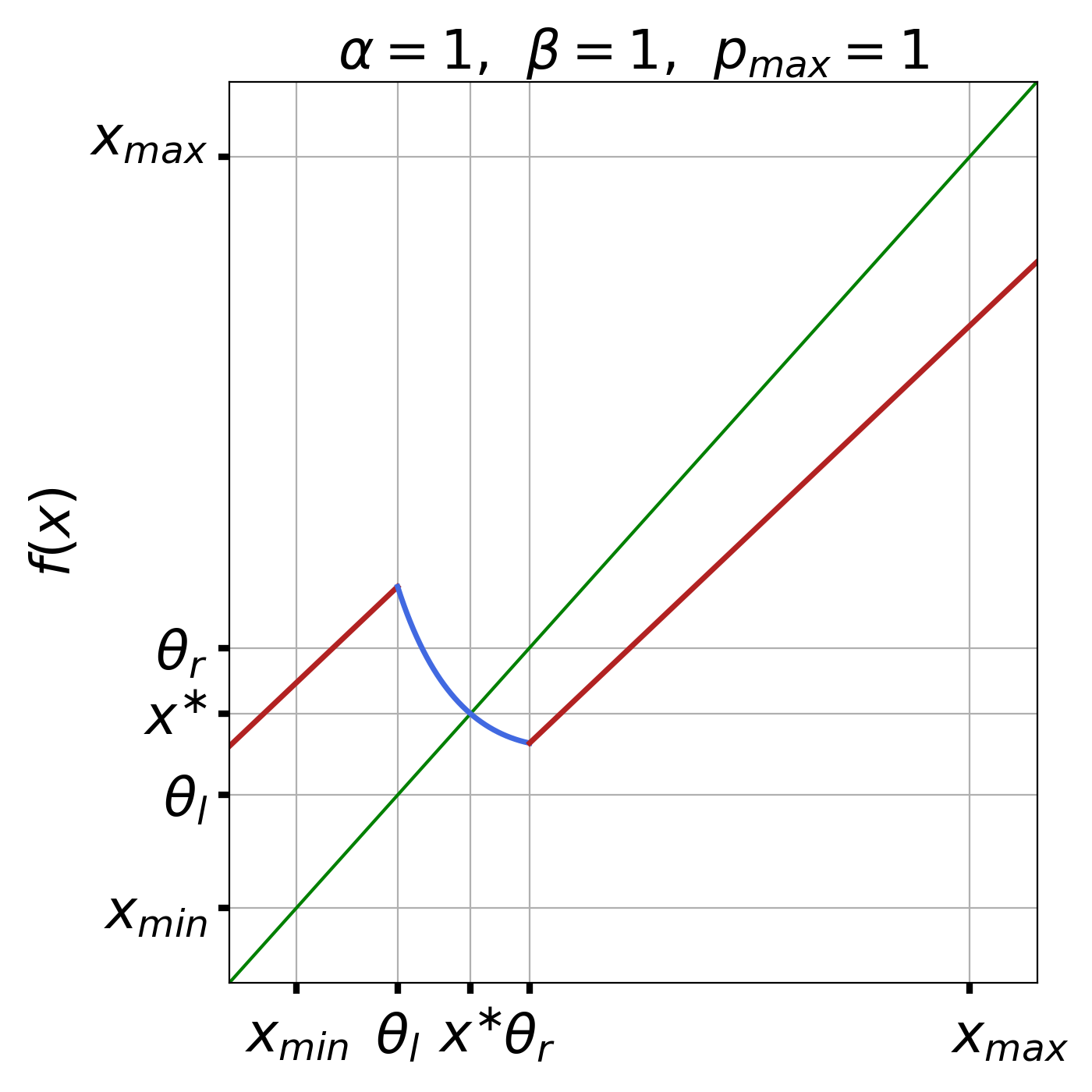
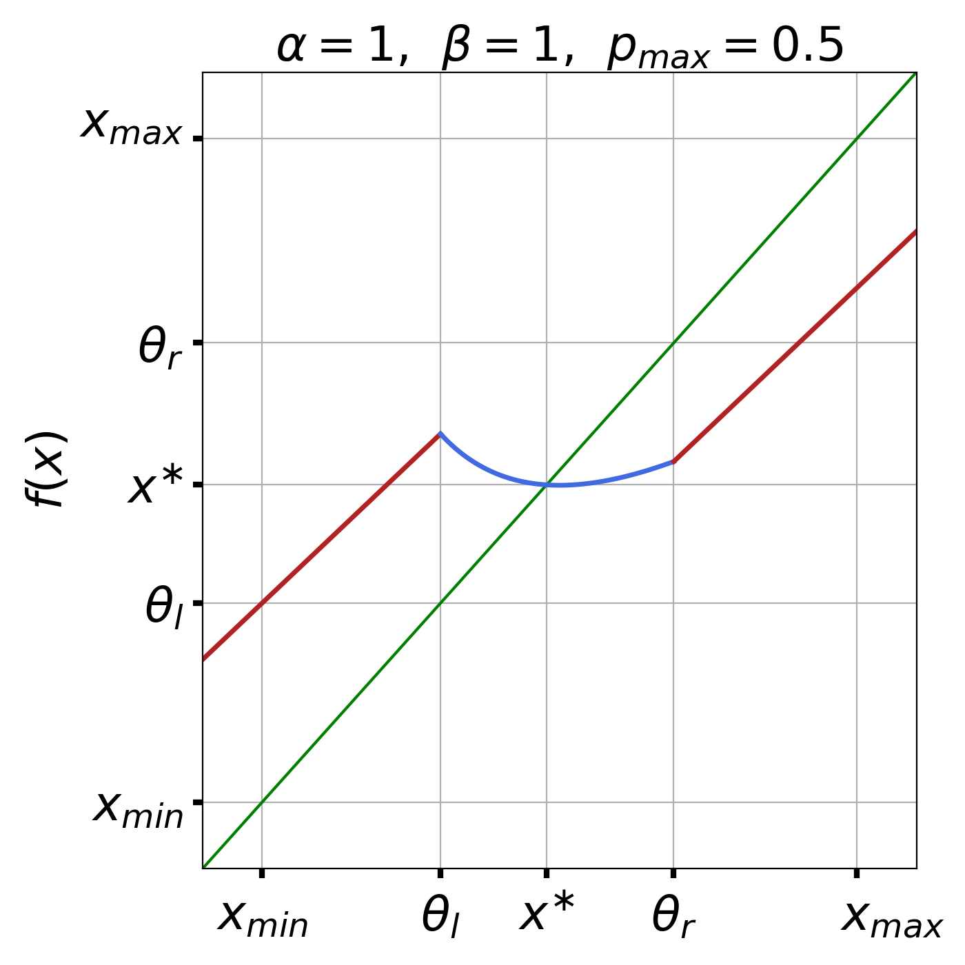
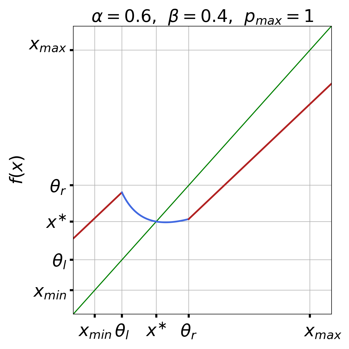
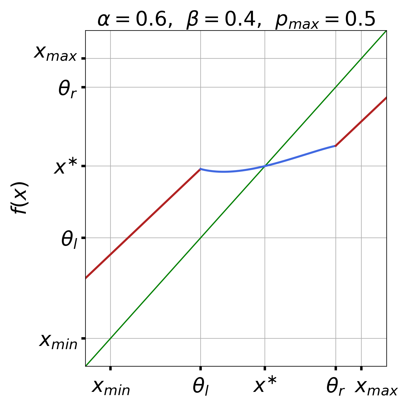
Figure 2: Graphs of the mapping $f$, Equation (27), for the values of $\alpha$, $\beta$ and $p_{\max}$ displayed at the top of the panels. Remaining parameters are given in (49) and (50). The restriction $\left.f\right|_{(\theta_{l},\theta_{r})}$ is monotonically decreasing in the upper left panel, while it is $\cup$-convex in the other panels.

Figures 3 and 4 show the bifurcation diagram and the Lyapunov exponent with respect to $x_{\min}$ and $x_{\max}$, respectively, obtained with the values $\alpha=\beta=1$ (upper row) and $\alpha=0.6$, $\beta=0.4$ (lower row) for the values $p_{\max}=1$ (left column) and $p_{\max}=0.5$ (right column). The settings of the other control parameters are given in the captions of the figures. For clarity, we also depict the endpoints $\theta_{l},\theta_{r}$ of the dynamical core, that encloses the fixed point $x^{\ast}$. The parametric grid used for the bifurcation diagrams has $2000$ points; the orbits were $550$ iterates long, the first $500$ (the transient) having been discarded.

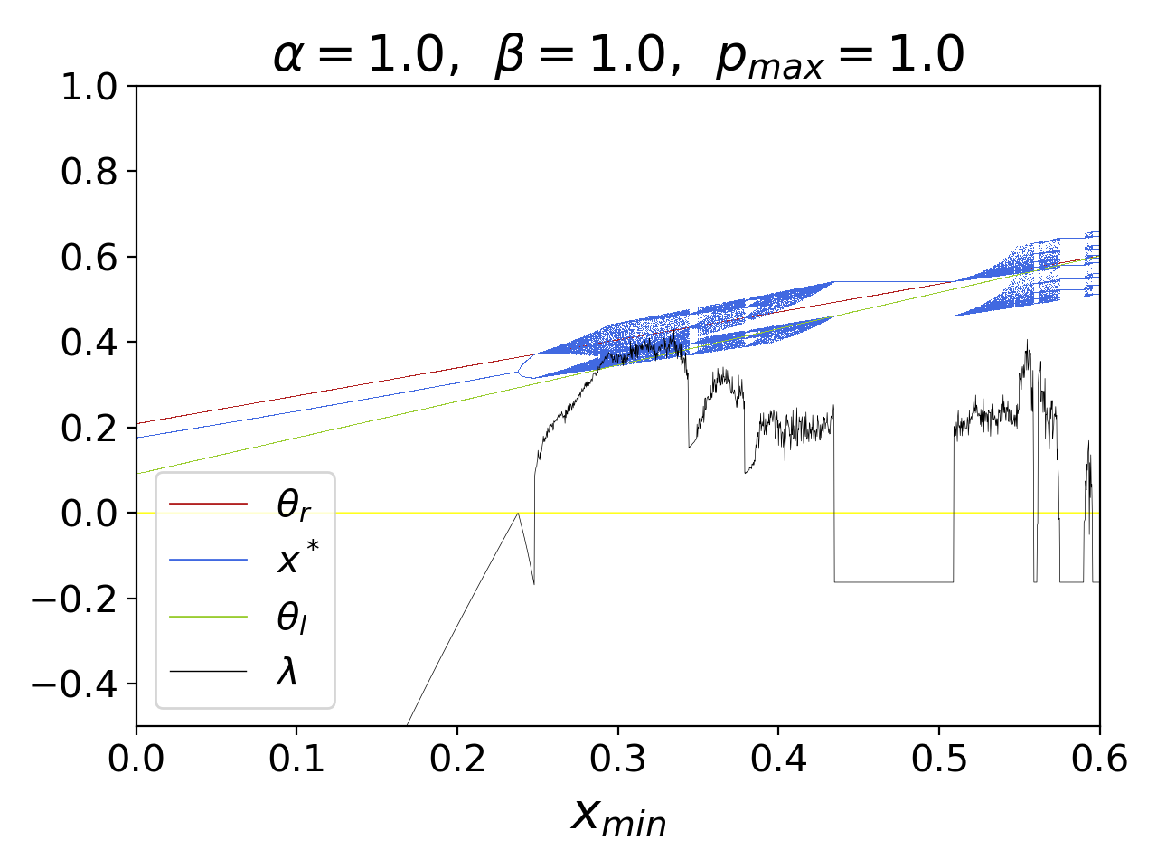
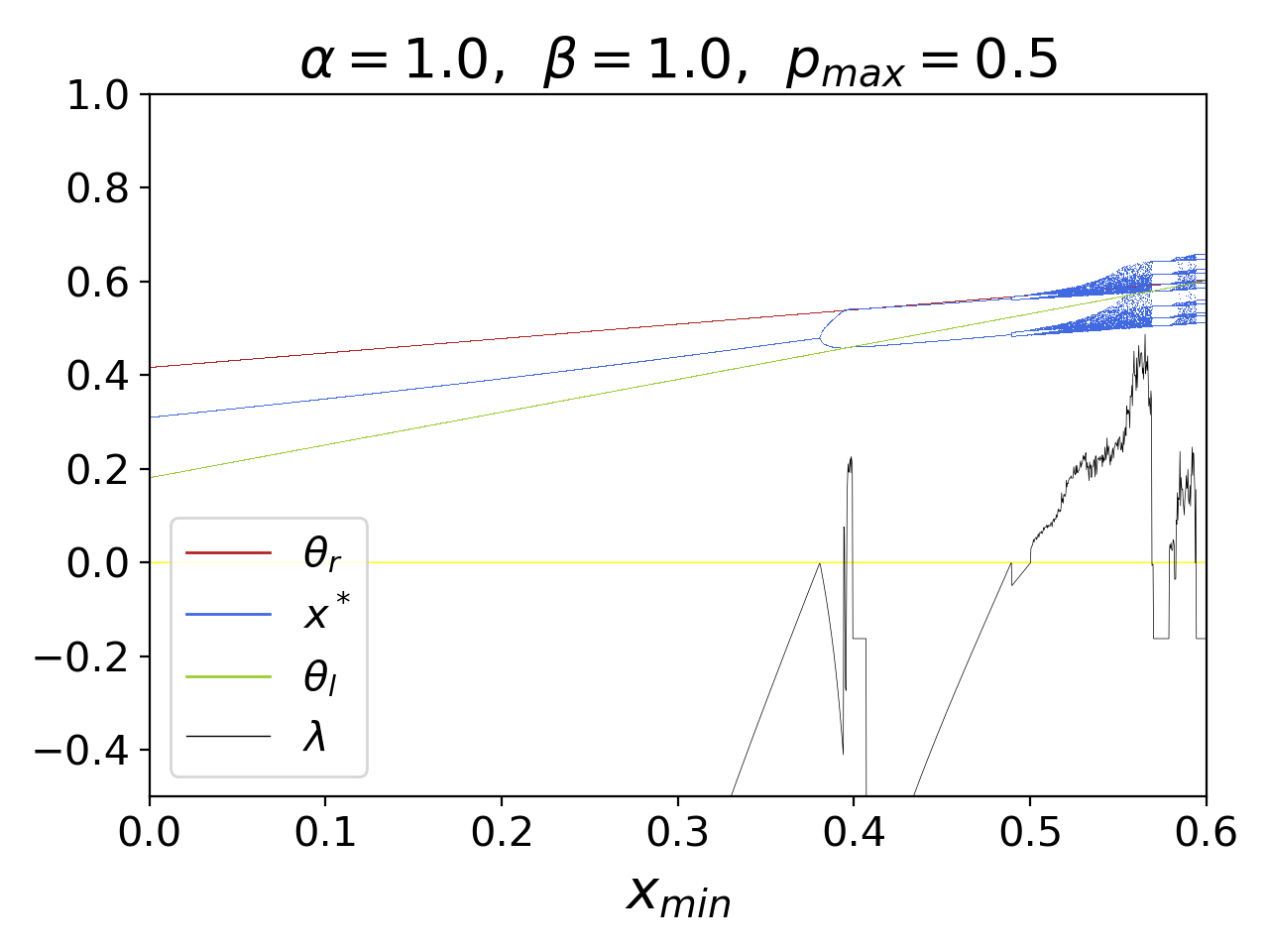
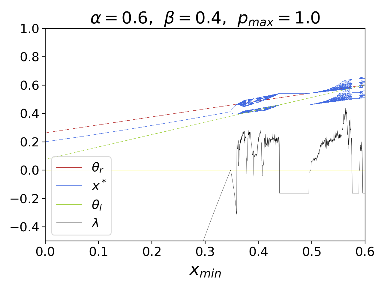
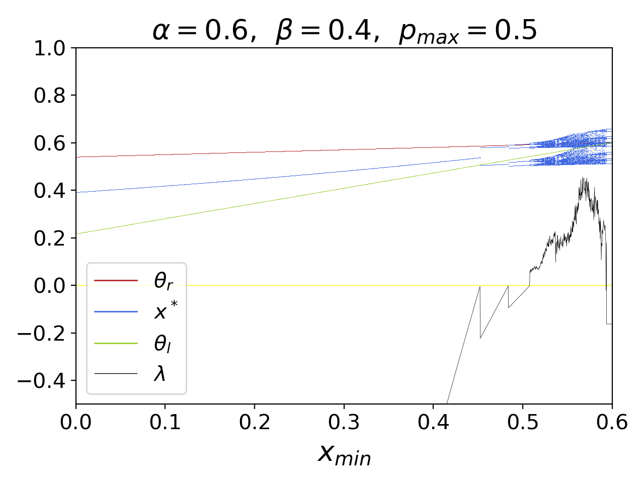
Figure 3: Bifurcation diagram and Lyapunov exponents of the normalized average queue length $x$ with respect to the parameter $x_{\min}$ for the values of $\alpha$, $\beta$ and $p_{\max}$ displayed at the top of the panels. The parameter $x_{\min}$ ranges in the interval $[0.2,0.6)$. System parameters are given in (49). Other control parameters: $x_{\max}=0.6$ and $w=0.15$.

The most salient aspects of these figures can be summarized as follows.

(1) The bifurcations are direct for $x_{\min}$ (i.e., for growing values), whereas they are reverse for $x_{\max}$ (i.e., for decreasing values).

(2) The bands of chaos start after the collision of an initial period-2 orbit with one of the endpoints of the dynamical core $(\theta_{l},\theta_{r})$. One speaks in this case of a boundary collision bifurcation.

(3) The bifurcation points with respect to $x_{\min}$ occur before for $p_{\max}=1$ than for $p_{\max}=0.5$. The opposite happens with respect to $x_{\max}$. In either case we conclude that the setting $p_{\max}=0.5$ is more robust than $p_{\max}=1.$

(4) Last but not least, the bifurcation point with respect to $x_{\min}$ (resp. $x_{\max}$) for $\alpha=0.6$, $\beta=0.4$ is greater (resp. smaller) than for $\alpha=\beta=1$. So the model with $\alpha=0.6$, $\beta=0.4$ is more stable with respect to both $x_{\min}$ and $x_{\max}$ than the original model (18).

Similar conclusions regarding the stability of $x^{\ast}$ were obtained in [3] with respect to $A_{1}$, $A_{2}$ and $w$.

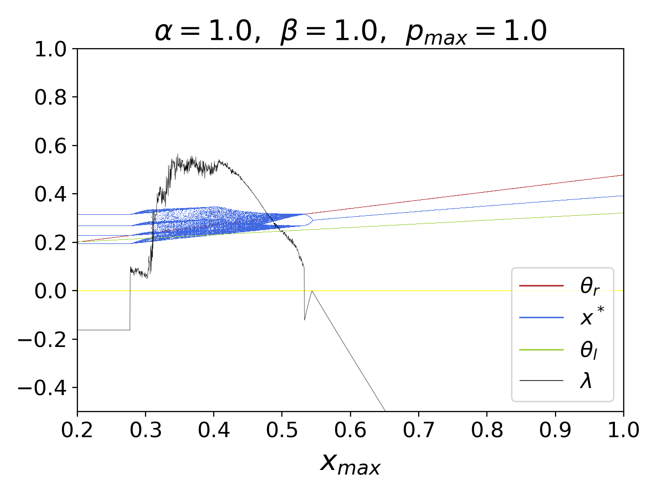
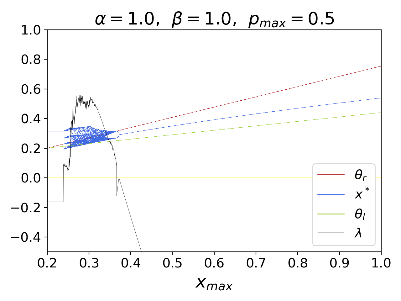
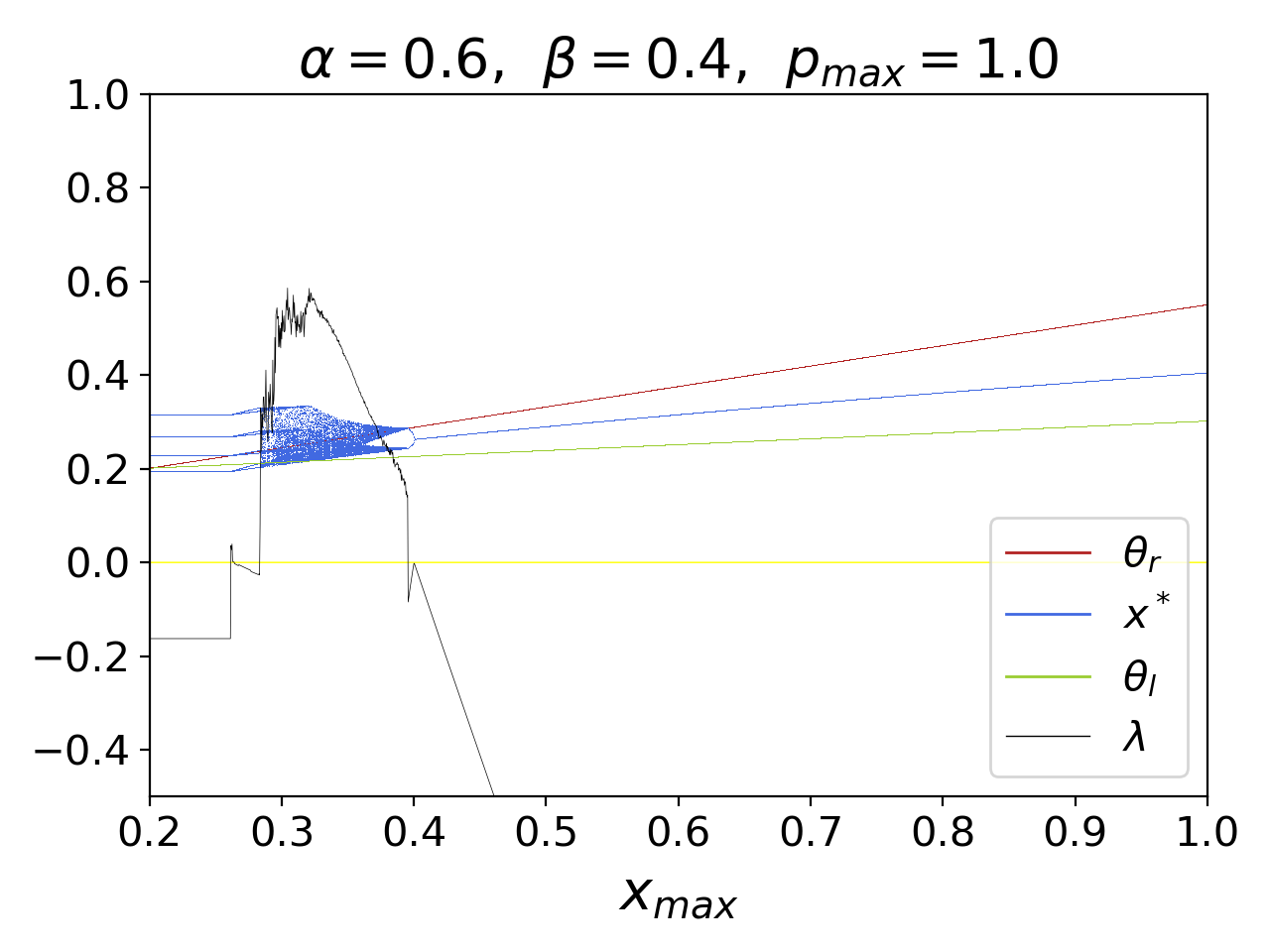
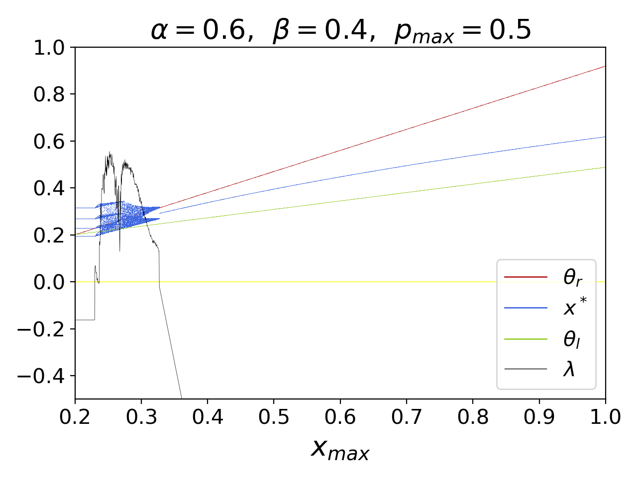
Figure 4: Bifurcation diagram and Lyapunov exponents of the normalized average queue length $x$ with respect to the parameter $x_{\max}$ for the values of $\alpha,\beta$ and $p_{\max}$ displayed at the top of the pannels. The parameter $x_{\max}$ ranges in the interval $(0.2,1]$. System parameters are given in (49). Other control parameters: $x_{\min}=0.2$ and $w=0.15$.

6.2 Robustness domains

Bifurcation diagrams are instrumental to find ranges of the control parameters that guarantee a stable dynamics. But this is not sufficient for our purposes. In this regard, an important feature in the design of AQM mechanisms is that small changes in the selected control parameters should not affect the stability of the system. In other words, the selected values of the control parameters (especially, $\alpha$ and $\beta$) should be also robust. As a result, robustness in the sense meant here, enables a stable operation under both changing system parameters and perturbations due to physical and numerical noise.

If bifurcations diagrams allow to find the stability ranges of different parameters, robustness domains allow to fine-tune the selection of control parameters for stability control under changing system parameters. In Figure 5 we have scanned the interval $[0.002,1.5]\times[0.002,1.5]$ of the $(\alpha,\beta)$-plane with precision $\Delta\alpha=\Delta\beta=3.745\times 10^{-3}$ (corresponding to a grid of $400\times 400$ points). For each point $(\alpha,\beta)$ we have calculated the bifurcation point of the averaging weight $w_{\mathrm{bif}}$ in two different scenarios according to the number of connections: $N=1350$ on the left panel and and $N=1850$ on the right panel.

Regarding the robustness domains shown in the left panel of Figure 5, we see that the second greatest domain corresponds to $0.15\leq w_{\mathrm{bif}}\leq 0.30$, and the third greatest to $0.30\leq w_{\mathrm{bif}}\leq 0.45$. Although the latter is smaller, settings of $\alpha,\beta$ in that domain (with a typical selection $\alpha=0.5$, $\beta=0.1$) leave an ample range $0<w<0.30$ for stable operation. Points $(\alpha,\beta)$ close to the boundaries of the robustness (same-color) domains should be avoided. Furthermore, comparison of the left panel with the right one shows that, as $N$ increases, corresponding domains overlap, so one can find suitable selections of $\alpha$ and $\beta$ for $N$ ranging from $1350$ to the reference number $1850$. The observation that the robustness domains with $w_{\mathrm{bif}}\geq 0.15$ shrinks as $N$ decreases agrees with the fact that a small number of connections (users) tends to disrupt the dynamics [19].

Of course, a thorough analysis is necessary for the actual design of an AQM algorithm. Our point here is that the decision on how to fix the control parameters is a compromise between the size of the robustness domains and stability ranges. We believe that the robustness domains are a handy tool for that endeavour.

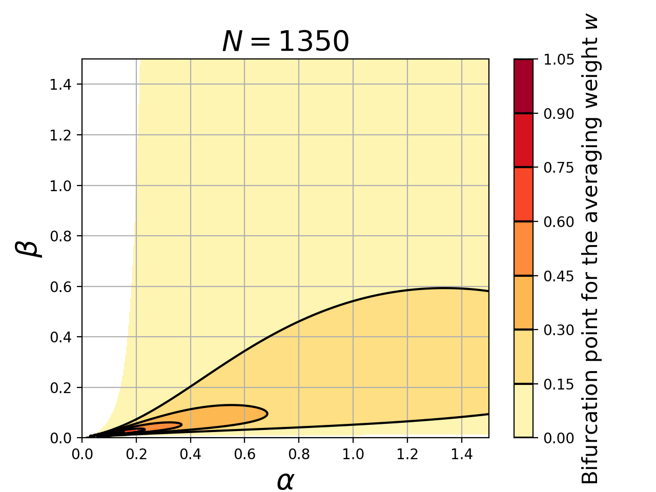
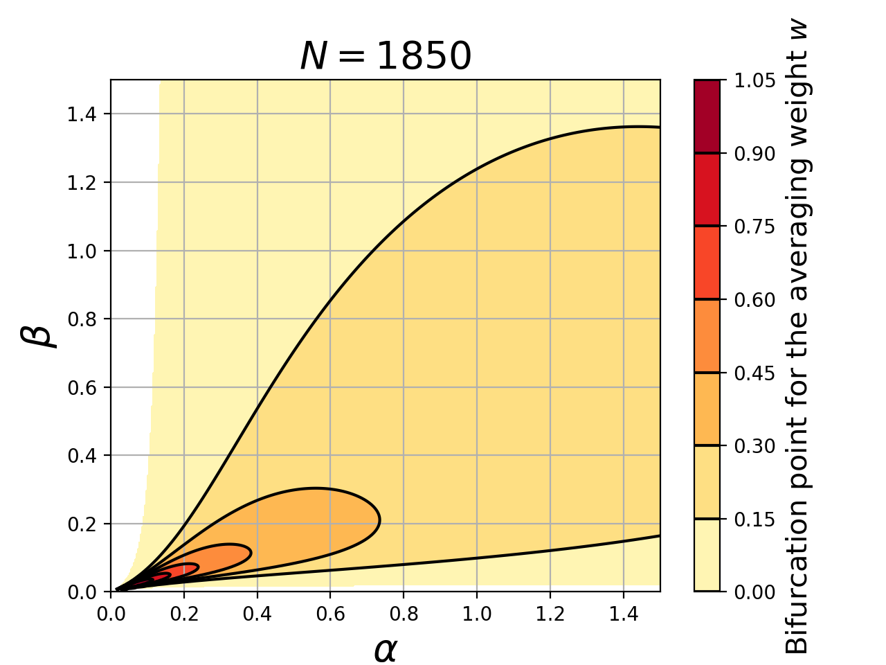
Figure 5: $(\alpha,\beta)$-parametric sweeps for the bifurcation point of the averaging weight $w$. Left panel: $N=1350$; Right panel: $N=1850$ (Source: [3]). Remaining system parameters are given in (49). Other control parameters: $x_{\min}=0.2$, $x_{\max}=0.6$.

7 Conclusion and outlook

Deterministic models (mostly involving continuous time and differential equations) are typical of the traditional sciences, in which the evolution laws can be derived from first principles. Stochastic models are usually put in place in the opposite case, i.e., when the laws governing a process are unknown, hence a data-driven description is the only option left. There are intermediate situations, though, where a deterministic description is possible but too complex to be of any practical use. A paradigmatic example is statistical mechanics, where the constituents move according to Newton’s laws and, yet, a probabilistic approach, where the observables are sample averages in phase space, is the best way to bridge the gap between the microscopic and the macroscopic scales. Other well-known example is symbolic dynamics, which is obtained by coarse-graining the state space of a discrete-time dynamical system.

In this paper we proceeded the other way around: the outset was RED, a stochastic model to manage the incoming packet queue at a router’s buffer. In this specific case, the uncertainty about the arrival times of the packets makes unfeasible a deterministic model. But if one contents oneself with aggregate information, which behaves in a more regular way, then the full power of a nonlinear model is available for prediction and control, showing that stochastic and deterministic models can complement each other advantageously. How to transit from the original RED model to a discrete-time dynamical formulation, where the states are average queue sizes at the buffer, was shown in Section 2. Since the resulting nonlinear version of RED turns out to be rather sensitive to the setting of control parameters (in particular, to the averaging weight $w$), the model was generalized in Section 3, Equation (27), by replacing the original RED probability law (1) for packet dropping by a new one, Equation (23), involving the beta distribution (24). This way, two new control parameters $\alpha$ and $\beta$ are added; for $\alpha=\beta=1$ one recovers the initial dynamical model (18). In Section 4 we gathered the main theoretical results on the global stability of $x^{\ast}$, the unique fixed point of the generalized RED model (27) if $A_{1}<A_{2}+x_{\max}$ (Theorem 3). Sufficient conditions were given in Theorem 8 for a monotone $f_{(\theta_{l},\theta_{r})}$, and in Theorems 9-10 for $f_{(\theta_{l},\theta_{r})}$ unimodal. Particular results for $f_{(\theta_{l},\theta_{r})}$ a $\cup$-convex function were derived in Section 5. The chaotic behavior of the RED dynamics, proved in Section 3, was quantified by bifurcation diagrams and Lyapunov exponents in Section 6.1, while the robustness of the fixed point under variations of the control parameters was discussed in Section 6.2.

The ultimate goal of the results reviewed and reported in this paper is the design of a congestion control algorithm for the data traffic on the Internet in a realistic environment, i.e., when some parameters of the communication network (notably, the number of users $M$ and the round-trip time $d$) may vary over time. This was the main reason for studying convex mappings in Section 5 and parametric robustness in Section 6.2. The former provide an interesting trade-off between the implementation of the analytical constraints and practical controllability; the latter is crucial if the control parameters (especially $\alpha$, $\beta$ and $w$) have to be adjusted in real time. Congestion control under real conditions is the subject of work in progress.

References

- [1] M. Abramowitz, I.A. Stegun, Handbook of Mathematical Functions, (Dover Publications, 1972).
- [2] R. Adams, Active Queue Management: A Survey, IEEE Communications Surveys and Tutorials 15 (2013) 1425–1476.
- [3] J.M. Amigó, G. Duran, A. Giménez, O. Martínez-Bonastre, J. Valero, Generalized TCP-RED dynamical model for Internet congestion control, Communications in Nonlinear Science and Numerical Simulation 82 (2020) 105075.
- [4] M. Arpaci, J.A. Copeland, An adaptive queue management method for congestion avoidance in TCP/IP networks, IEEE Global Telecommunications Conference (Globecom’00), Conference Record (Cat. No.00CH37137), 1 (2000) 309–315.
- [5] S. Athuraliya, V.H. Li, S.H. Low, Q. Yin, REM: Active queue management, Teletraffic Science and Engineering, (Elsevier, 2001).
- [6] C. Brandauer, G. Iannaccone, C. Diot, T. Ziegler, S. Fdida, M. May, Comparison of tail drop and active queue management performance for bulk-data and Web-like Internet traffic, Proceedings of the Sixth IEEE Symposium on Computers and Communications, (2001) 122–129.
- [7] K. Chin-Fu, Sao-Jie Chen, Jan-Ming Ho, Ray-I Chang, Improving end-to-end performance by active queue management, 19th International Conference on Advanced Information Networking and Applications (AINA’05) Volume 1 (AINA papers), 2 (2005) 337–340.
- [8] M. Claypool, R. Kinicki, M. Hartling, Active queue management for Web traffic, IEEE International Conference on Performance, Computing, and Communications, (2004) 531–538.
- [9] G. Duran, J. Valero, J.M. Amigó, A. Giménez, O. Martínez-Bonastre, Stabilizing Chaotic Behavior of RED, 2018 IEEE 26th International Conference on Network Protocols (ICNP), (2018) 241–242.
- [10] G. Duran, J. Valero, J.M. Amigó, A. Giménez, O. Martinez-Bonastre, Bifurcation analysis for the Internet congestion, 2019 IEEE Conference on Computer Communications Workshops (INFOCOM), (2019) 1073–1074.
- [11] H.A. El-Morshedy, E. Liz, Globally attracting fixed points in higher order discrete population models, J. Math. Biol. 53 (2006) 365–384.
- [12] S. Floyd, V. Jacobson, Random early detection gateways for congestion avoidance, IEEE/ACM Trans. Networking 1 (1993) 397–413.
- [13] S. Floyd, R. Gummadi, S. Shenker, Adaptive RED: An Algorithm for Increasing the Robustness of RED’s Active Queue Management, Online, (2001) 1–12.
- [14] J.P. Hespanha, S. Bohacek, K. Obraczka, J. Lee, Hybrid Modeling of TCP Congestion Control, Hybrid Systems: Computation and Control, (2001) 291–304.
- [15] T. Li, J.A. Yorke, Period Three Implies Chaos, Amer. Math. Monthly 82 (1975) 985–992.
- [16] M. Mathis, J. Semke, J. Mahdavi, T. Ott, The Macroscopic Behavior of the TCP Congestion Avoidance Algorithm, SIGCOMM Comput. Commun. Rev. 27 (1997) 67–82.
- [17] J. Padhye, V. Firoiu, D. Towsley, J. Kurose, Modeling TCP Reno performance: a simple model and its empirical validation, IEEE/ACM Transactions on Networking 8 (2000) 133–145.
- [18] P. Ranjan, E.H. Abed, R.J. La, Nonlinear instabilities in TCP-RED, Proc. IEEE INFOCOM, (2002) 249–258.
- [19] P. Ranjan, E.H. Abed, R.J. La, Nonlinear instabilities in TCP-RED, IEEE/ACM Transactions on Networking 12 (2004) 1079–1092.
- [20] A.N. Sharkovskiĭ, Coexistence of cycles of a continuous map of the line into itself, Ukranian Mathematical Journal 16 (1964) 61–71.
- [21] W. Wang, H. Wang, W. Tang, F. Guo, A New Approach to Estimate RED Parameters Using Function Regression, International Journal of Future Generation Communication and Networking 7 (2014) 103–118.