A Unified Optimization Framework for Low-Rank Inducing Penalties

Abstract

In this paper we study the convex envelopes of a new class of functions. Using this approach, we are able to unify two important classes of regularizers from unbiased non-convex formulations and weighted nuclear norm penalties. This opens up for possibilities of combining the best of both worlds, and to leverage each methods contribution to cases where simply enforcing one of the regularizers are insufficient.

We show that the proposed regularizers can be incorporated in standard splitting schemes such as Alternating Direction Methods of Multipliers (ADMM), and other subgradient methods. Furthermore, we provide an efficient way of computing the proximal operator.

Lastly, we show on real non-rigid structure-from-motion (NRSfM) datasets, the issues that arise from using weighted nuclear norm penalties, and how this can be remedied using our proposed method.

1 Introduction

Dimensionality reduction using Principal Component Analysis (PCA) is widely used for all types of data analysis, classification and clustering. In recent years, numerous subspace clustering methods have been proposed, to address the shortcomings of traditional PCA methods. The work on Robust PCA by Candès et al. [6] is one of the most influential papers on the subject, which sparked a large research interest from various fields including computer vision. Applications include, but are not limited to, rigid and non-rigid structure-from-motion [4, 1], photometric stereo [2] and optical flow [12].

It is well-known that the solution to

$$\min_{\operatorname{rank}(X)\leq r}\left\|X-X_{0}\right\|_{F}^{2},$$ (1)

where $\left\|\cdot\right\|_{F}$ is the Frobenius norm, can be given in closed form using the singular value decomposition (SVD) of the measurement matrix $X_{0}$. The character of the problem changes drastically, when considering objectives such as

$$\min_{\operatorname{rank}(X)\leq r}\left\|\mathcal{A}(X)-\mathbf{b}\right\|^{2},$$ (2)

where $\mathcal{A}\>:\>\mathbbm{R}^{m\times n}\rightarrow\mathbbm{R}^{p}$ is a linear operator, $\mathbf{b}\in\mathbbm{R}^{p}$, and $\left\|\cdot\right\|$ is the standard Euclidean norm. In fact, such problems are in general known to be NP hard [13]. In many cases, however, the rank is not known a priori, and a “soft rank” penalty can be used instead

$$\min_{X}\mu\operatorname{rank}(X)+\left\|\mathcal{A}(X)-\mathbf{b}\right\|^{2}.$$ (3)

Here, the regularization parameter $\mu$ controls the trade-off between enforcing the rank and minimizing the residual error, and can be tuned to problem specific applications.

In order to treat objectives of the form (2) and (3), a convex surrogate of the rank penalty is often used. One popular approach is to use the nuclear norm [26, 6]

$$\left\|X\right\|_{*}=\sum_{i=1}^{n}\sigma_{i}(X),$$ (4)

where $\sigma_{i}(X)$, $i=1,\ldots,n$, is the $i$:th singular value of $X$. One of the drawbacks of using the nuclear norm penalty is that both large and small singular values are penalized equally hard. This is referred to as shrinking bias, and to counteract such behavior, methods penalizing small singular values (assumed to be noise) harder have been proposed [25, 20, 15, 23, 24, 18, 9, 28].

1.1 Related Work

Our work is a generalization of Larsson and Olsson [18]. They considered problems on the form

$$\min_{X}g(\operatorname{rank}(X))+\left\|X-X_{0}\right\|_{F}^{2},$$ (5)

where the regularizer $g$ is non-decreasing and piecewise constant,

$$g(k)=\sum_{i=1}^{k}g_{i}.$$ (6)

Note, that for $g_{i}\equiv\mu$ we obtain (3). Furthermore, if we let $g_{i}=0$ for $i\leq r_{0}$, and $\infty$ otherwise, (2) is obtained. The objectives (5) are difficult to optimize, as they, in general, are non-convex and discontinuous. Thus, it is natural to consider a relaxation

$$\min_{X}\mathcal{R}_{g}(X)+\left\|X-X_{0}\right\|_{F}^{2},$$ (7)

where

$$\mathcal{R}(X)=\max_{Z}\left(\sum_{i=1}^{n}\min(g_{i},\sigma_{i}^{2}(Z))-\left\|X-Z\right\|_{F}^{2}\right).$$ (8)

This is the convex envelope of (5), hence share the same global minimizers.

Another type of regularizer that has been successfully used in low-level imaging applications [14, 32, 31] is the weighted nuclear norm (WNNM),

$$\left\|X\right\|_{\mathbf{w},*}=\sum_{i=1}^{k}w_{i}\sigma_{i}(X),$$ (9)

where $\mathbf{w}=(w_{1},\ldots,w_{k})$ is a weight vector. Note that the WNNM formulation does not fit the assumptions (6), hence cannot be considered in this framework.

For certain applications, it is of interest to include both regularizers, which we will show in Section 6. Typically, this is preferable when the rank constraint alone is not strong enough to yield accurate reconstructions, and further penalization is necessary to restrict the solutions. To this end, we suggest to merge these penalties. Our main contributions are:

• A novel method for combining bias reduction and non-convex low-rank inducing objectives,

• An efficient and fast algorithm to compute the proposed regularizer,

• Theoretical insight in the quality of reconstructed missing data using WNNM, and practical demonstrations on how shrinking bias is perceived in these applications,

• A new objective for Non-Rigid Structure from Motion (NRSfM), with improved performance, compared to state-of-the-art prior-free methods, capable of working in cases where the image sequences are unordered.

First, however, we will lay the ground for the theory of a common framework of low-rank inducing objectives.

2 Problem Formulation and Motivation

In this paper we propose a new class of regularization terms for low rank matrix recovery problems that controls both the rank and the size of the singular values of the recovered matrix. Our objective function has the form

$$f_{h}(X)=h(\bm{\sigma}{(}X))+\|\mathcal{A}(X)-b\|^{2},$$ (10)

where $h(\bm{\sigma}{(}X))=\sum_{i=1}^{k}h_{i}(\sigma_{i}(X))$ and

$$h_{i}(\sigma_{i}(X))=\begin{cases}2a_{i}\sigma_{i}(X)+b_{i}&\sigma_{i}(X)\neq 0,\\ 0&\text{otherwise}.\end{cases}$$ (11)

We assume that the sequences $\{a_{i}\}_{i=1}^{k}$ and $\{b_{i}\}_{i=1}^{k}$ are both non-decreasing.

Our approach unifies the formulation of [17] with weighted nuclear norm. The terms $2a_{i}\sigma_{i}(X)$ correspond to the singular value penalties of a weighted nuclear norm [14]. These can be used to control the sizes of the non-zero singular values. In contrast, the constants $b_{i}$ corresponds to a rank penalization that is independent of these sizes and, as we will see in the next section, enables bias free rank selection.

2.1 Controlled Bias and Rank Selection

To motivate the use of both sets of variables $\{a_{i}\}_{i=1}^{k}$ and $\{b_{i}\}_{i=1}^{k}$, and to understand their purpose, we first consider the simple recovery problem $\min_{X}f_{h}(X)$, where

$$f_{h}(X)\coloneqq h(\bm{\sigma}{(}X))+\|X-X_{0}\|_{F}^{2}.$$ (12)

Here $X_{0}$ is assumed to consist of a set of large singular values $\sigma_{i}(X_{0})$, $i=1,...,r$, corresponding to the matrix we wish to recover, and a set of small ones $\sigma_{i}(X_{0})$, $i=r+1,...,k$, corresponding to noise that we want to suppress.

Due to von Neumann’s trace theorem the solution can be computed in closed form by considering each singular values separately, and minimize

$$\begin{cases}2a_{i}s+b_{i}+(s-\sigma_{i}(X_{0}))^{2}&s\neq 0,\\ \sigma_{i}(X_{0})^{2}&s=0,\end{cases}$$ (13)

over $s\geq 0$. Differentiating for the case $s\neq 0$ gives a stationary point at $s=\sigma_{i}(X)-a_{i}$ if $\sigma_{i}(X)-a_{i}>0$. Since this point has objective value $2a_{i}\sigma_{i}(X_{0})-a_{k}^{2}+b_{k}$ it is clear that this point will be optimal if

$$2a_{i}\sigma_{i}(X_{0})-a_{i}^{2}+b_{i}\leq\sigma_{i}(X_{0})^{2},$$ (14)

or equivalently $\sigma_{i}(X_{0})-a_{i}\geq\sqrt{b_{i}}.$ Summarizing, we thus get the optimal singular values

$$\sigma_{i}(X)=\begin{cases}\sigma_{i}(X_{0})-a_{i}&\sigma_{i}(X_{0})-a_{i}\geq\sqrt{b_{i}},\\ 0&\text{otherwise}.\end{cases}$$ (15)

Note, that this is a valid sequence of singular values since under our assumptions $\sigma_{i}(X_{0})-a_{i}$ is decreasing and $\sqrt{b_{i}}$ increasing. The red curve of Figure 1 shows the recovered singular value as a function of the corresponding observed singular value. For comparison, we also plot the dotted blue curve which shows hard thresholding at $a_{i}+\sqrt{b}_{i}$, i.e. singular values smaller than $a_{i}+\sqrt{b}_{i}$ vanish while the rest are left unaltered.

Figure 1: The optimal recovered singular value $\sigma_{i}(X)$ as a function (red curve) of the observed $\sigma_{i}(X_{0})$.

Now, suppose that we want to recover the largest singular values unchanged. Using the weighted nuclear norm ($b_{i}=0$) it is clear that this can only be done if we know that the sought matrix has rank $r$ and let $a_{i}=0$ for $i=1,...,r$. For any other setting the regularization will subtract $a_{i}$ from the corresponding non-zero singular value. In contrast, by letting $a_{i}=0$ allows exact recovery of the large singular values by selecting $b_{i}$ appropriately even when the rank is unknown. Hence, in the presence of a weak prior on the rank of the matrix, using only the $b_{i}$ (the framework in [18]) allows exact recovery for a more general set of problems than use of the $a_{i}$ (weighted nuclear norm formulations).

The above class of problems are well posed with a strong data term $\|X-X_{0}\|_{F}^{2}$. For problems with weaker data terms, priors on the size of the singular values can still be very useful. In the context of NRSfM it has been observed [24, 11] that adding a bias can improve the distance to the ground truth reconstruction, even though it does not alter the rank. The reason is that, when the scene is not rigid, several reconstructions with the same rank may co-exist, thus resulting in similar projections. By introducing bias on the singular values, further regularization is enforced on the deformations, which may aid in the search for correct reconstructions. For example, with $a_{1}=0$ and $a_{i}>0$, $i>1$ we obtain a penalty that favors matrices that ”are close to” rank $1$. In the formulation of [11], where rank $1$ corresponds to a rigid scene this can be thought of as an ”as rigid as possible” prior, which is realistic in many cases [27, 21], but which has yet to be considered in the context of factorization methods.

2.2 The Quadratic Envelope

As discussed above the two sets of parameters $\{a_{i}\}$ and $\{b_{i}\}$ have complementary regularization effects. The main purpose of unifying them is to create more flexible priors allowing us to do accurate rank selection with a controlled bias. In the following sections, we also show that they have relaxations that can be reliably optimized. Specifically, the resulting formulation $h(\bm{\sigma}{(X)})$, which is generally non-convex and discontinuous, can be relaxed by computing the so called quadratic envelope [10]. The resulting relaxation $\mathcal{R}_{h}(\bm{\sigma}{(}X))$ is continuous and in addition $\mathcal{R}_{h}(\bm{\sigma}{(}X))+\|X-X_{0}\|_{F}^{2}$ is convex. For a more general data term there may be multiple local minimizers. However, it is known that

$$h(\bm{\sigma}{(}X))+\|\mathcal{A}(X)-b\|^{2},$$ (16)

and

$$\mathcal{R}_{h}(\bm{\sigma}{(}X))+\|\mathcal{A}(X)-b\|^{2},$$ (17)

have the same global minimizer when $\|\mathcal{A}\|<1$ [10]. In addition, potential local minima of (17) are also local minima of (16); however, the converse does not hold. We also show that the proximal operator of $\mathcal{R}_{h}(\bm{\sigma}{(}X))$ can be efficiently computed which allows simple optimization using splitting methods such as ADMM [3].

3 A New Family of Functions

Consider functions on the form (12). This is a generalization of [18]; and the derivation for our objective follows a similar structure. We outline this in detail in the supplementary material, where we show that convex envelope $f^{**}_{h}$ is given by

$$f^{**}_{h}(X)=\mathcal{R}_{h}(X)+\left\|X-X_{0}\right\|_{F}^{2},$$ (18)

where

$$\mathcal{R}_{h}(X) \coloneqq\max_{Z}\Bigg{(}\sum_{i=1}^{n}\min\left(b_{i},\left[\sigma_{i}(Z)-a_{i}\right]_{+}^{2}\right)+\left\|Z\right\|_{F}^{2}$$ (19)

$$-\left\|X-Z\right\|_{F}^{2}-\sum_{i=1}^{n}\left[\sigma_{i}(Z)-a_{i}\right]_{+}^{2}\Bigg{)}.$$

Furthermore, the optimization can be reduced to the singular values only,

$$\mathcal{R}_{h}(X) =\max_{\bm{\sigma}{(}Z)}\Bigg{(}\sum_{i=1}^{n}\min\left(b_{i},\left[\sigma_{i}(Z)-a_{i}\right]_{+}^{2}\right)+\sigma_{i}^{2}(Z)$$ (20)

$$-(\sigma_{i}(X)-\sigma_{i}(Z))^{2}-\left[\sigma_{i}(Z)-a_{i}\right]_{+}^{2}\Bigg{)}.$$

This optimization problem is concave, hence can be solved with standard convex solvers such as MOSEK or CVX; however, in the next section we show that the problem can be turned into a series of one-dimensional problems, and the resulting algorithm for computing (19) is magnitudes faster than applying a general purpose solver.

4 Finding the Maximizing Sequence

Following the approach used in [18], consider the program

$$\max_{s} f(s)$$ (21)

s.t. $$\sigma_{i+1}(Z)\leq s\leq\sigma_{i-1}(Z).$$

where $\sigma_{i}(Z)$ is the $i$:th singular value of the maximizing sequence in (20), and

$$f(s)=\min\{b_{i},[s-a_{i}]_{+}^{2}\}-(s-\sigma_{i}(X))^{2}+s^{2}-[s-a_{i}]_{+}^{2}.$$ (22)

The objective function $f$ can be seen as the pointwise minimum of two concave functions, namely, $f_{1}(s)=b_{i}+2\sigma_{i}(X)s-\sigma_{i}^{2}(X)-[s-a_{i}]_{+}^{2}$ and $f_{2}(s)=2\sigma_{i}(X)s-\sigma_{i}(X)^{2}$, i.e. $f(s)=\min\{f_{1}(s),f_{2}(s)\}$, hence $f$ is concave.

The individual unconstrained optimizers are given by $s_{i}=a_{i}+\max\{\sqrt{b_{i}},\sigma_{i}(X)\}$. In previous work [18], where $a_{i}\equiv 0$, an algorithm was devised to find the maximizing singular vector, by turning it to a optimization problem of a single variable. This method is not directly applicable, as the sequence $\{s_{i}\}_{i=1}^{k}$, in general, does not satisfy the necessary conditions. In fact, the number of local extrema in the sequence $\{s_{i}\}_{i=1}^{k}$ is only limited by its length. We show an example of a sequence in Figure 2, and the corresponding maximizing sequence. Nevertheless, it is possible to devise an algorithm that returns the maximizing singular value vector, as we will show shortly.

In order to do so, we can apply some of the thoughts behind the proof behind [18]. Consider the more general optimization problem of minimizing $g(\bm{\sigma})=\sum_{i=1}^{k}f_{i}(s_{i})$, subject to $\sigma_{1}\geq\sigma_{2}\geq\cdots\geq\sigma_{k}\geq 0$, where $f_{i}$ are concave. Then, given the unconstrained sequence of minimizers $\{s_{i}\}_{i=1}^{k}$, the elements of the constrained sequence $\{\sigma_{i}\}_{i=1}^{k}$ can be limited to three choices

$$\sigma_{i}=\left\{\begin{aligned} &s_{i}&&\text{ if }\sigma_{i+1}\leq s_{i}\leq\sigma_{i-1},\\ &\sigma_{i-1}&&\text{ if }\sigma_{i-1}<s_{i},\\ &\sigma_{i+1}&&\text{ if }s_{i}<\sigma_{i+1}.\\ \end{aligned}\right.$$ (23)

Furthermore, the regions between local extreme points (of the unconstrained singular values) are constant.

Lemma 1.

Assume $s_{p}$ and $s_{q}$ are local extrema of $\{s_{i}\}_{i=1}^{k}$ and that the subsequence $\{s_{i}\}_{i=p}^{q}$ are non-decreasing. Then the corresponding subsequence of the constrained problem $\{\sigma_{i}\}_{i=p}^{q}$ is constant.

Proof.

Consider $\sigma_{i}$ for some $p\leq i\leq q-1$. If $\sigma_{i}>s_{i}$, then by (23) we have $\sigma_{i+1}=\sigma_{i}$. If instead $\sigma_{i}\leq s_{i}$, we have $\sigma_{i+1}\leq\sigma_{i}\leq s_{i}\leq s_{i+1}$ and by (23), $\sigma_{i+1}=\sigma_{i}$. ∎

Data: Weights $\mathbf{a}$, $\mathbf{b}$, and $\bm{\sigma}{(}X)$

Result: Maximizing vector $\bm{\sigma}{(}Z^{*})=\{\sigma_{i}\}_{i}$

Initialize with the unconstrained maximizers $\sigma_{i}=a_{i}+\max\{\sqrt{b_{i}},\sigma_{i}(X)\}$;

while $\bm{\sigma}{(}Z^{*})$ is not a valid singular value vector do

       Find local extrema of $\bm{\sigma}{(}Z^{*})$ and generate subintervals $\{\iota_{k}\}_{k\in\mathcal{I}}$;

       for $k\in\mathcal{I}$ do

             Find scalar $s^{*}=\operatorname*{arg\,max}_{s}f(s)$ where $f$ is defined in (22);

             Update $\sigma_{i}=s^{*}$ for all $i\in\iota_{k}$.

       end for

      

end while

Algorithm 1 Algorithm for finding the maximizing singular value vector.

We can now devise an algorithm that returns the maximizing sequence, see Algorithm 1. Essentially, the algorithm starts at the unconstrained solution, and then adds more constraints, by utilizing Lemma 1, until all of them are fulfilled.

Theorem 1.

Algorithm 1 returns the maximizing sequence.

Proof.

See the supplementary material. ∎

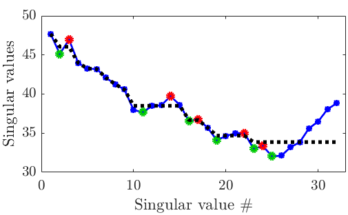
Figure 2: Example of a sequence of unconstrained maximizers (blue line), local extrema (green and red) and the maximizing sequences (dashed black) obtained by Algorithm 1.

Table 1: Distance to ground truth (normalized) mean valued over 20 problem instances for different percentages of missing data and data patterns. The standard deviation of the noise is kept constant at $\sigma=0.1$. Best results are marked in bold.

Missing
data (%)	PCP [7]	WNNM [14]	Unifying [5]	LpSq [22]	S12L12 [28]	S23L23 [28]	IRNN [9]	APGL [29]	$\left\|\cdot\right\|_{*}$ [3]	$\mathcal{R}_{\mu}$ [18]	Our
0	0.0400	0.0246	0.0406	0.0501	0.0544	0.0545	0.0551	0.0229	0.1959	0.0198	0.0199
20	0.3707	0.2990	0.3751	0.1236	0.1322	0.0972	0.0440	0.0233	0.2287	0.0257	0.0198
40	1.0000	0.6185	0.9355	0.1265	0.1222	0.1137	0.0497	0.0291	0.3183	0.2105	0.0248
60	1.0000	0.8278	1.0000	0.1354	0.1809	0.1349	0.0697	0.0826	0.5444	0.3716	0.0466
Uniform AA 80	1.0000	0.9810	1.0000	0.7775	0.6573	0.5945	0.2305	0.4648	0.8581	0.9007	0.3117
0	0.0399	0.0220	0.0399	0.0491	0.0352	0.0344	0.0491	0.0205	0.1762	0.0176	0.0177
10	0.3155	0.2769	0.1897	0.1171	0.0881	0.0874	0.0926	0.1039	0.2607	0.0829	0.0802
20	0.4681	0.4250	0.3695	0.1893	0.1346	0.1340	0.1430	0.1686	0.3425	0.2146	0.1343
30	0.5940	0.5143	0.4147	0.1681	0.2822	0.3081	0.1316	0.1594	0.3435	0.4137	0.1277
40	0.7295	0.6362	0.9331	0.2854	0.4262	0.4089	0.1731	0.2800	0.5028	0.5072	0.1705
Tracking AA 50	0.7977	0.7228	0.9162	0.4439	0.5646	0.5523	0.2847	0.4219	0.5831	0.6464	0.3128

5 ADMM and the Proximal Operator

We employ the splitting method ADMM [3], which is a standard tool for problems of this type. Thus, consider the augmented Lagrangian

$$L(X,Y,\Lambda)=f_{h}^{**}(X)+\rho\left\|X-Y+\Lambda\right\|_{F}^{2}+{\mathcal{C}}(Y)-\rho\left\|\Lambda\right\|_{F}^{2}.$$ (24)

In each iteration, we solve

$$X_{t+1} =\operatorname*{arg\,min}_{X}f_{h}^{**}(X)+\rho\left\|X-Y_{t}+\Lambda_{t}\right\|_{F}^{2},$$ (25)

$$Y_{t+1} =\operatorname*{arg\,min}_{Y}\rho\left\|X_{t+1}-Y+\Lambda_{t}\right\|_{F}^{2}+{\mathcal{C}}(Y),$$ (26)

$$\Lambda_{t+1} =X_{t+1}-Y_{t+1}+\Lambda_{t}.$$ (27)

To evaluate the proximal operator $f_{h}^{**}$ one must solve

$$\min_{X}\mathcal{R}_{h}(X)+\left\|X-X_{0}\right\|_{F}^{2}+\rho\left\|X-M\right\|_{F}^{2}.$$ (28)

Note, that due to the definition of (19), this can be seen as a convex-concave min-max problem, by restricting the minimization of $X$ over a compact set. By first solving for $X$ one obtains,

$$X=M+\frac{X_{0}-Z}{\rho}=\frac{(\rho+1)Y-Z}{\rho},$$ (29)

where $Y=\frac{X_{0}+\rho M}{1+\rho}$. Similarly, as in [18], we get a program of the type (excluding constants)

$$\max_{Z}\Bigg{(}\sum_{i=1}^{n}\min\left(b_{i},\left[\sigma_{i}(Z)-a_{i}\right]_{+}^{2}\right)-\frac{\rho+1}{\rho}\left\|Z-Y\right\|_{F}^{2}$$ (30)

$$\qquad+\left\|Z\right\|_{F}^{2}-\sum_{i=1}^{n}\left[\sigma_{i}(Z)-a_{i}\right]_{+}^{2}\Bigg{)}.$$

Again, the optimization can be reduced to the singular values only. This bears strong resemblance to (21), and we show in the supplementary material that Algorithm 1 can be modified, with minimal effort, to solve this problem as well.

6 Experiments

We demonstrate the shortcomings of using WNNM for non-rigid reconstruction estimation and structure-from-motion, and show that our proposed method performs as good or better than the current state-of-the-art. In all applications, we apply the popular approach [8, 14, 16] to choose the weights inversely proportional to the singular values,

$$w_{i}=\frac{C}{\sigma_{i}(X_{0})+\epsilon},$$ (31)

where $\epsilon>0$ is a small number (to avoid division by zero), and $X_{0}$ is an initial estimate of the matrix $X$. The trade-off parameter $C$ will be tuned to the specific application. In the experiments, we use $w_{i}=2a_{i}$, and choose $b_{i}$ depending on the specific application. This allows us to control the rank of the obtained solution without excessive penalization of the non-zero singular values.

6.1 Synthetic Missing Data

In this section we consider the missing data problem with unknown rank

$$\min_{X}\mu\operatorname{rank}(X)+\left\|W\odot(X-M)\right\|_{F}^{2},$$ (32)

where $M$ is a measurement matrix, $\odot$ denotes the Hadamard (or element-wise) product, and $W$ is a missing data mask, with $w_{ij}=1$ if the entry $(i,j)$ is known, and zero otherwise.

Ground truth matrices $M_{0}$ of size $32\times 512$ with $\operatorname{rank}(M_{0})=4$ are generated, and to simulate noise, a matrix $N$ is added to obtain the measurement matrix $M=M_{0}+N$. The entries of the noise matrix are normally distributed with zero mean and standard deviation $\sigma=0.1$.

When benchmarking image inpainting and deblurring, it is common to assume a uniformly distributed missing data pattern. This assumption, however, is not applicable in many other subfields of computer vision. In structure-from-motion the missing data pattern is typically very structured, due to tracking failures. For comparison we show the reconstruction results for several methods, on both uniformly random missing data patterns and tracking failures. The tracking failure patterns were generated as in [19]. The results are shown in Table 1. Here we use the $a_{i}=\frac{\sqrt{\mu}}{\sigma_{i}(M)+\epsilon}$, and $b_{i}=\frac{\mu}{\sigma_{i}(M)+\epsilon}$, with $\epsilon=10^{-6}$. All other parameters are set as proposed by the respective authors.

6.2 Non-Rigid Deformation with Missing Data

This experiment is constructed to highlight the downsides of using WNNM, and to illustrate how shrinking bias can manifest itself in a real-world application. Non-rigid deformations can be seen as a low-rank minimizing problem by assuming that the tracked image points are moving in a low-dimensional subspace. This allows us to model the points using a linear shape basis, where the complexity of the motion is limited by the number of basis elements. This in turn, leads to the task of accurately making trade-offs while enforcing a low (and unknown) rank, which leads to the problem formulation

$$\min_{X}\mu\operatorname{rank}(X)+\left\|W\odot(X-M)\right\|,$$ (33)

where $X=CB^{T}$, with $B$ being concatenated basis elements and $C$ the corresponding coefficient matrix. We use the experimental setup from [17], where a KLT tracker is used on a video sequence. The usage of the tracker naturally induces a structured missing data pattern, due to the inability to track the points through the entire sequence.

We consider the relaxation of (33)

$$\min_{X}\mathcal{R}_{h}(X)+\left\|W\odot(X-M)\right\|_{F}^{2},$$ (34)

and choose $a_{i}=\frac{C}{\sigma_{i}(M)+\epsilon}$ and $b_{i}=0$ for $i\leq 3$ and $b_{i}=1/(C+\epsilon)$ otherwise. This choice of $\mathbf{b}$ encourages a rank 3 solution without penalizing the large singular values, and by choosing the parameter $C$ vary the strength of the fix rang regularization versus the weighted nuclear norm penalty. The datafit vs the parameter $C$ is shown in Table 2, and the reconstructed points for four frames of the book sequence are shown in Figure 3.

Notice that, the despite the superior datafit for $C=1$ (encouraging the WNNM penalty), it is clear by visual inspection that the missing points are suboptimally recovered. In Figure 3 the white center marker is the origin, and we note a tendency for the WNNM penalty to favor solutions where the missing points are closer to the origin. This is the consequence of a shrinking bias, and is only remedied by leaving the larger singular values intact, thus excluding WNNM as a viable option for such applications.

Table 2: Datafit for different values of $C$. Note that the datafit for $C=1$ is better than for $C=10^{-2}$. This comes at the cost of incorrectly reconstructing the missing points, as is shown in Figure 3. The datafit is measured as $\left\|W\odot(X-M)\right\|_{F}$.

$C$	$10^{-2}$	1	100
Datafit	0.8354	0.4485	6.5221

Frame 1	Frame 121	Frame 380	Frame 668

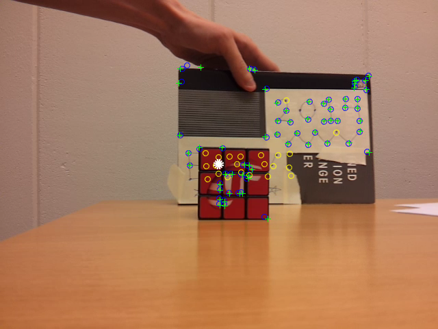
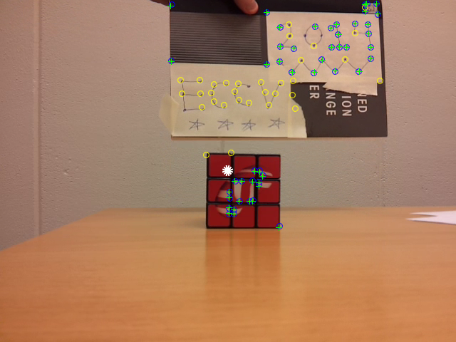
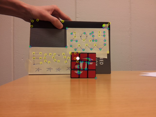
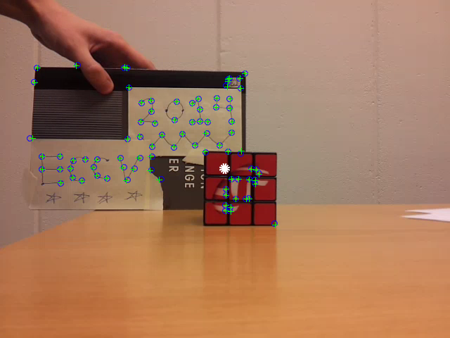
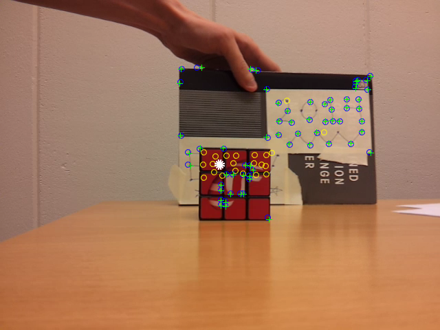
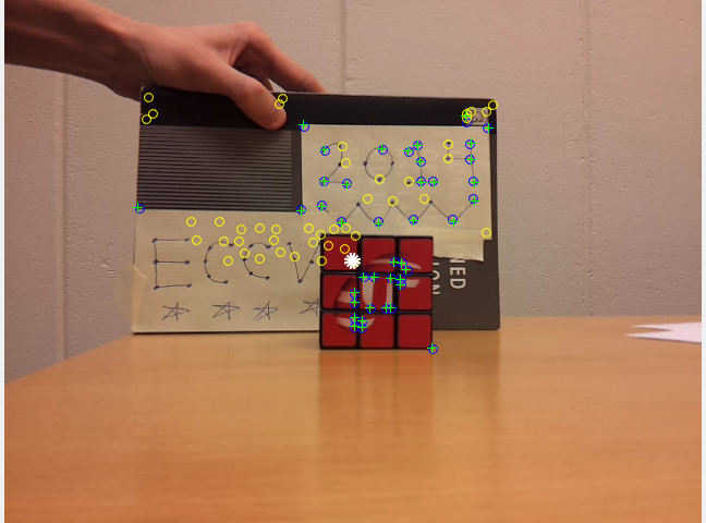
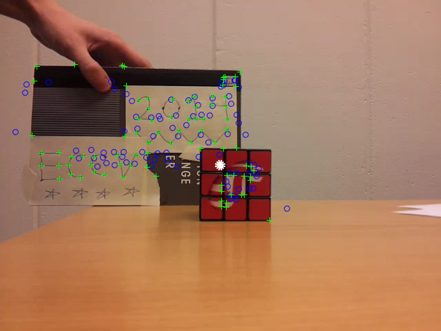
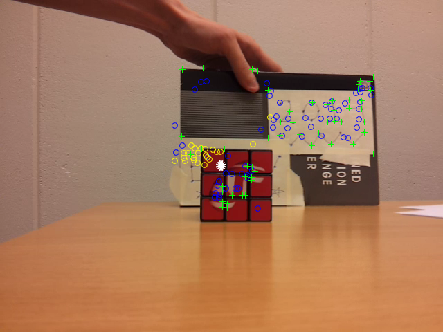
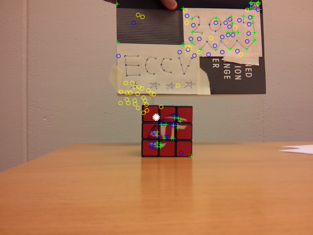
Figure 3: From top to bottom, $C=10^{-2}$, $C=1$ and $C=100$. The white center dot is the origin in the chosen coordinate system. The green crosses show the observed data, and the blue dots the reconstruction of these points. The yellow dots correspond to the recovered (and missing) data. Notice the shrinking bias which is evident due to the recovered missing data being drawn towards the center of the image as the WNNM penalty increases.

6.3 Motion Capture

The popular prior-free objective, proposed by Dai et al. [11], for NRSfM

$$\min_{X}\mu\left\|X^{\sharp}\right\|_{*}+\left\|RX-M\right\|_{F}^{2},$$ (35)

where $X^{\sharp}$ a stacked version of $X$ (see [11] for details), suffers from shrinking bias, due to the nuclear norm penalty. Essentially, the nuclear norm penalty is a way of relaxing the soft rank penalty,

$$\min_{X}\mu\operatorname{rank}(X^{\sharp})+\left\|RX-M\right\|_{F}^{2},$$ (36)

however, it was shown in [24], that simply using the convex envelope of the rank function leads to non-physical reconstructions. To tackle this situation, it was proposed to penalize the 3D trajectories using a difference operator $D$,

$$\min_{X}\mu\operatorname{rank}(X^{\sharp})+\left\|RX-M\right\|_{F}^{2}+\left\|DX^{\sharp}\right\|_{F}^{2}.$$ (37)

While such an objective leads to more physical solutions [24], it also restricts the method to ordered sequences of images. To allow for unordered sequences, we suggest to replace the difference operator with an increasing penalty for smaller singular values, modelled by an increasing sequence of weights $\{a_{i}\}$. More specifically, we consider the problem of minimizing

$$\min_{X}\mathcal{R}_{h}(X^{\sharp})+\left\|RX-M\right\|_{F}^{2},$$ (38)

where sequences $\{a_{i}\}$ and $\{b_{i}\}$ are non-decreasing. This bears resemblance to the weighted nuclear norm approach presented in [16], recently, which coincide for the special case $b_{i}\equiv 0$. Furthermore, this modified approach exhibits far superior reconstruction results compared to the original method proposed by Dai et al. [11]. In our comparison, we employ the same initialization heuristic for the weights $w_{i}$ on the singular values as in [14, 16], namely

$$w_{i}=\frac{C}{\sigma_{i}(X_{0}^{\sharp})+\epsilon},$$ (39)

where $\epsilon=10^{-6}$ and $C>0$. The matrix $X_{0}^{\sharp}=R^{+}M$, where $R^{+}$ is the pseudo-inverse of $R$, has successfully been used as an initialization scheme for NRSfM by others [11, 30, 16].

In practice, we choose $2a_{i}=w_{i}$, as in (39), with $C=2\sqrt{\mu}$ and $b_{i}=w_{i}$, with $C=\mu$. This enforces mixed a soft-rank and hard rank thresholding.

We select four sequences from the CMU MOCAP dataset, and compare to the original method proposed by Dai et al. [11], the newly proposed weighted approach by Kumar [16], the method by Larsson and Olsson [18] and our proposed objective (38), all of which are prior-free, and do not assume that the image sequences are ordered. For the nuclear norm approach by Dai et al. we use the regularization parameter $\lambda=2\sqrt{\mu}$, and for Kumar, we set $C=2\sqrt{\mu}$ (as for $\mathcal{R}_{h}$) and run the different methods for a wide range of values for $\mu$, using the same random initial solutions. We then measure the datafit, defined as $\left\|RX-M\right\|_{F}$ and the distance to ground truth $\left\|X-X_{\text{gt}}\right\|_{F}$, and show how these depend on the output rank (here defined as the number of singular values larger than $10^{-6}$). By doing so, we see the ability of the method to make accurate trade-offs between fitting the data and enforcing the rank. The results are shown in Figure 4.

Note that, the datafit for all methods decrease with increase rank, which is to be expected; however, we immediately note that the “soft rank” penalty (3), in this case, is too weak, which manifests itself by quickly fitting to data and the distance to ground truth does not correlate with the datafit for solutions with rank larger than three. For the revised method by Kumar [16], as well as ours, the correlation between the two quantities is much stronger. What is interesting to see is that our method consistently performs better than the WNNM approach for lower rank levels, suggesting that the shrinking bias is affecting the quality of these reconstruction. Note, however, that the minimum distance to ground truth, obtained using the WNNM approach is as good (or better) than the one obtained using $\mathcal{R}_{h}$. To obtain such a solution, however, requires careful tuning of the $\mu$ parameter and is unlikely to work on other datasets.

Drink
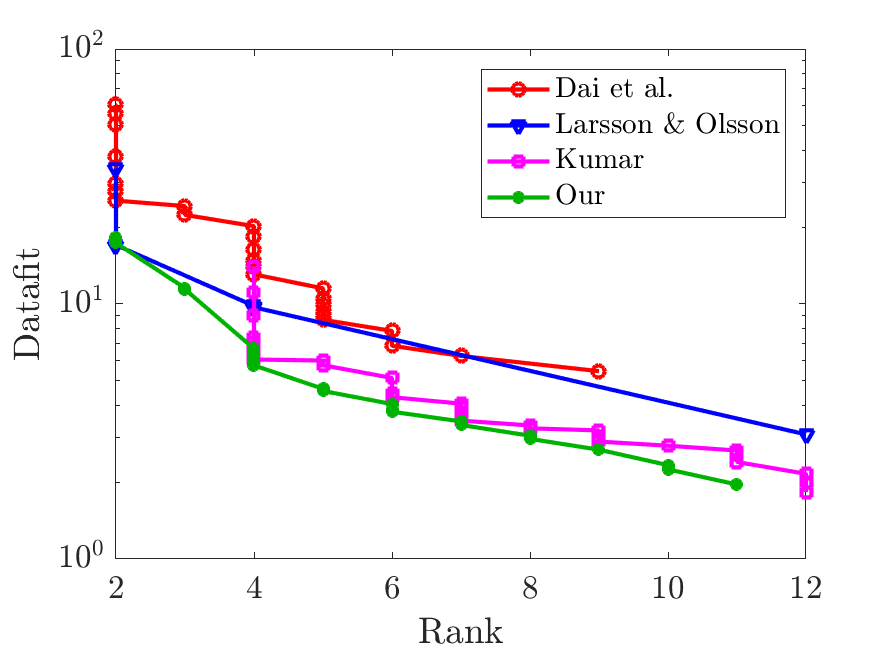
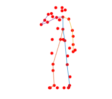
Pickup
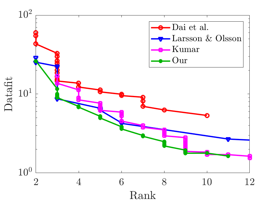
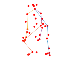
Stretch
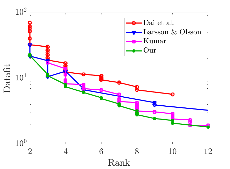
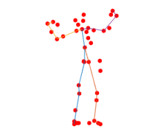
Yoga

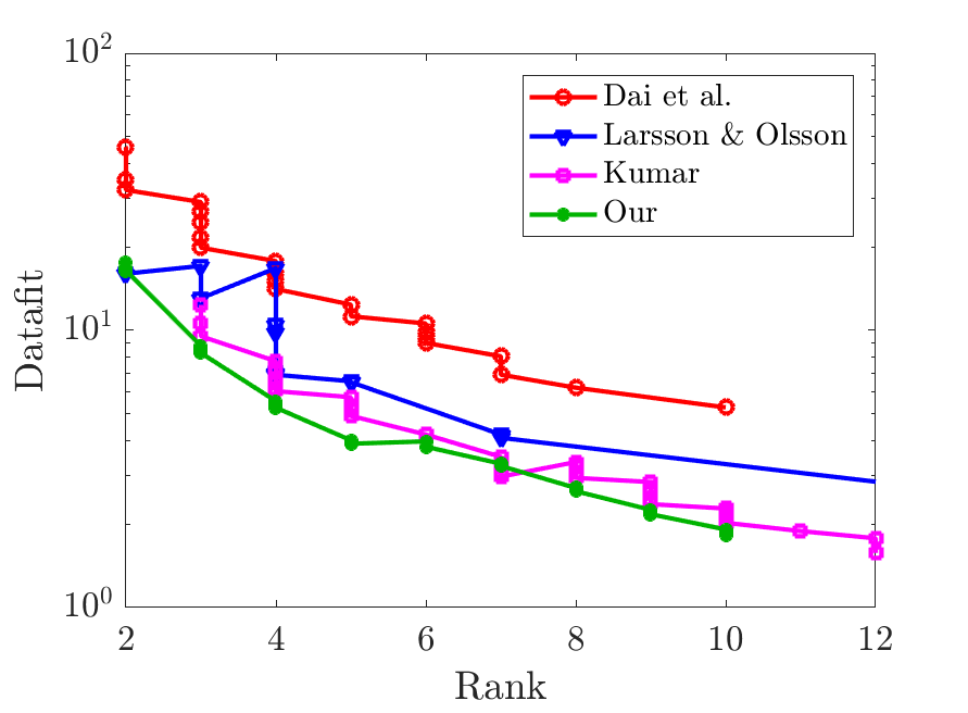
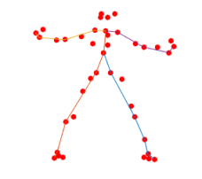
Figure 4: Results for the experiment on the CMU MOCAP dataset. First column: Example images with skeleton added for visualization. Second column: The datafit, measured as $\left\|RX-M\right\|_{F}$, as a function of the rank. Last column: Distance to ground truth, measured as $\left\|X-X_{\text{gt}}\right\|_{F}$, as a function of the rank.

7 Conclusions

Despite success in many low-level imaging applications, there are limitations of the applicability of WNNM in other applications of low-rank regularization. In this paper, we have provided theoretical insight into the issues surrounding shrinking bias, and proposed a solution where the shrinking bias can be partly or completely eliminated, while keeping the rank low. This can be done using the proposed $\mathcal{R}_{h}$ regularizer, which has the benefit of unifying weighted nuclear norm regularization with another class of low-rank inducing penalties. Furthermore, an efficient way of computing the regularizer has been proposed, as well as the related proximal operator, which makes it suitable for optimization using splitting scheme, such as ADMM.

Supplementary Material:
A Unified Optimization Framework for Low-Rank Inducing Penalties

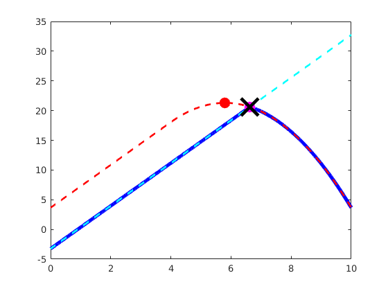
Figure 5: Two different cases for values of $a_{i}$, $b_{i}$ and $\sigma_{i}(X)$ of (21).

1 The Fenchel Conjugate

In this section, we compute the Fenchel conjugate of (12), which is necessary in order to find the convex envelope. Let $\langle X,Y\rangle=\operatorname{tr}(X^{T}Y)$, and note that we can write

$$\langle Y,X\rangle-\left\|X-X_{0}\right\|_{F}=\left\|Z\right\|_{F}^{2}-\left\|X_{0}\right\|_{F}^{2}-\left\|Z-X\right\|_{F}^{2}.\\$$ (40)

where $Z=\frac{1}{2}Y+X_{0}$. By definition, the Fenchel conjugate of (12) is given by

$$f^{*}_{h}(Y) =\sup_{X}\langle Y,X\rangle-f_{h}(X)$$ (41)

$$=\sup_{X}\left\|Z\right\|_{F}^{2}-\left\|X_{0}\right\|_{F}^{2}-\left\|X-Z\right\|_{F}^{2}-h(\bm{\sigma}{(}X)),$$

where we use (40) in the last step. Note that the function $h$, as well as the Frobenius norm, is unitarily invariant. Furthermore, $\left\|X-Z\right\|_{F}^{2}=\left\|X\right\|_{F}^{2}+\left\|Z\right\|_{F}^{2}-2\langle X,Z\rangle$, and $\langle X,Z\rangle\leq\langle\bm{\sigma}{(}X),\bm{\sigma}{(}Z)\rangle$ by von Neumann’s trace inequality, with equality if $X$ and $Z$ are simultaneously unitarily diagonalizable. This reduces the problem to optimizing over the singular values alone, which, after some manipulation, can be written as

$$f^{*}_{h}(Y) =\max_{\bm{\sigma}{(}X)}-\left\|X_{0}\right\|_{F}^{2}$$ (42)

$$\quad-\sum_{i=1}^{k}\left(\sigma_{i}^{2}(X)-2[\sigma_{i}(Z)-a_{i}]\sigma_{i}(X)+b_{i}\right),$$

where $\operatorname{rank}(X)=k$. Considering each singular value separately leads to a program on the form

$$\min_{x_{i}}x_{i}^{2}-2[\sigma_{i}(Z)-a_{i}]x_{i}+b_{i},$$ (43)

subject to $\sigma_{i+1}(X)\leq x_{i}\leq\sigma_{i-1}(X)$. The sequence of unconstrained minimizers is given by $x_{i}=\sigma_{i}(Z)-a_{i}$. If there exists $x_{i}<0$, then this is not the solution to the constrained problem. Nevertheless, the sequence is non-increasing, hence there is an index $p$, such that $x_{p}\geq 0$ and $x_{p+1}<0$.

Note that

$$\sum_{i=1}^{k}x_{i}^{2}-2s_{i}x_{i}=\left\|\mathbf{x}\right\|^{2}-2\langle\mathbf{x},\mathbf{s}\rangle,$$ (44)

hence we can consider optimizing $\left\|\mathbf{x}-\mathbf{s}\right\|^{2}=\left\|\mathbf{x}\right\|^{2}-2\langle\mathbf{x},\mathbf{s}\rangle+\left\|\mathbf{s}\right\|^{2}$ subject to $x_{1}\geq x_{2}\geq\cdots\geq x_{k}\geq 0$. Furthermore, $s_{1}\geq s_{2}\geq\cdots\geq s_{k}$.

Assume that minimum is obtained at $\mathbf{x}^{*}$ and fix $x_{p}^{*}$. Since $s_{j}<0$ for all $j>p$, we must have $x^{*}_{j}=0$ for $j>p$. It is now clear that, $x_{j}^{*}=s_{j}$ otherwise, hence $x_{j}^{*}=\max\{s_{j},0\}=[s_{j}]_{+}$. Inserting into (42) gives

$$f^{*}_{h}(Y)=\max_{k}-\left\|X_{0}\right\|_{F}^{2}-\sum_{i=1}^{k}\left(b_{i}-[\sigma_{i}(Z)-a_{i}]_{+}^{2}\right).$$ (45)

Since $[s_{i}]_{+}=[\sigma_{i}(Z)-a_{i}]_{+}$ is non-increasing, and $b_{i}$ is non-decreasing, the maximizing $k$ is obtained when

$$[\sigma_{k}(Z)-a_{k}]_{+}^{2}\geq b_{k}\text{\, and\, }b_{k+1}\geq[\sigma_{k+1}(Z)-a_{k+1}]_{+}^{2}.$$ (46)

For the maximizing $k=k^{*}$, we can write

$$-\sum_{i=1}^{k^{*}}\left(b_{i}-[\sigma_{i}(Z)-a_{i}]_{+}^{2}\right)$$ (47)

$$\quad=\sum_{i=1}^{n}[\sigma_{i}(Z)-a_{i}]_{+}^{2}-\sum_{i=1}^{n}\min\{b_{i},[\sigma_{i}(Z)-a_{i}]_{+}^{2}\}.$$

From this observation, we get

$$f^{*}_{h}(Y) =\sum_{i=1}^{n}\left[\sigma_{i}(\frac{1}{2}Y+X_{0})-a_{i}\right]_{+}^{2}-\left\|X_{0}\right\|_{F}^{2}$$ (48)

$$-\sum_{i=1}^{n}\min\left(b_{i},\left[\sigma_{i}(\frac{1}{2}Y+X_{0})-a_{i}\right]_{+}^{2}\right).$$

2 The Convex Envelope

Applying the definition of the bi-conjugate $f^{**}_{h}(X)=\sup_{Y}\langle Y,X\rangle-f^{*}_{h}(Y)$ to (48), and introduce the change of variables $Z=\frac{1}{2}Y+X_{0}$ we get

$$f^{**}_{h}(X) =\max_{Z}2\langle X,Z-X_{0}\rangle-\sum_{i=1}^{n}\left[\sigma_{i}(Z)-a_{i}\right]_{+}^{2}$$ (49)

$$+\left\|X_{0}\right\|_{F}^{2}+\sum_{i=1}^{n}\min\left(b_{i},\left[\sigma_{i}(Z)-a_{i}\right]_{+}^{2}\right).$$

By expanding squares and simplifying, $2\langle X,Z-X_{0}\rangle+\left\|X_{0}\right\|_{F}^{2}=\left\|X-X_{0}\right\|_{F}^{2}-\left\|X-Z\right\|_{F}^{2}+\left\|Z\right\|_{F}^{2}$, which yields (19).

3 Obtaining the Maximizing Sequences

In this section we give the proof for the convergence of Algorithm 1, and how to modify it to cope with the corresponding problem for the proximal operator.

3.1 Proof of Theorem 1

Proof of Theorem 1.

First, we will show that each step in the algorithm returns a solution to a constrained subproblem $P_{i}$, corresponding to a (partial) set of desired constraints $\mathcal{Z}_{i}$.

Let $P_{0}$ denote the unconstrained problem with solution $\mathcal{s}\in\mathbbm{R}_{+}^{n}$. Denote the first interval generated in Algorithm 1 by $\iota_{1}=\{m_{1},\ldots,n_{1}\}$, and consider optimizing the first subproblem $P_{1}$

$$\max_{z_{m_{1}}\geq\cdots\geq z_{n_{1}}}c(\mathbf{z}),$$ (50)

where $\mathcal{Z}_{1}=\{\mathbf{z}\in\mathcal{Z}_{0}\,|\,z_{m_{1}}\geq\cdots\geq z_{n_{1}}\}$. By Lemma 1 the solution vector is constant over the subinterval $z_{i}=s$ for $i\in\iota_{1}$, which is returned by the algorithm. The next steps generates a solution to subproblem of the form

$$\max_{\scriptsize\begin{matrix}z_{m_{1}}\geq\cdots\geq z_{n_{1}}\\ \vdots\\ {z_{m_{k}}\geq\cdots\geq z_{n_{k}}}\end{matrix}}c(\mathbf{z}),$$ (51)

corresponding to subproblem $P_{k}$. I the solution to subproblem $P_{k}$ is in $\mathcal{Z}$, then it is a solution to the problem, otherwise one must add more constraints. We solve problems on the form

$$\max_{\mathbf{z}\in\mathcal{Z}_{0}}c(\mathbf{z})\geq\max_{\mathbf{z}\in\mathcal{Z}_{1}}c(\mathbf{z})\geq\cdots\geq\max_{\mathbf{z}\in\mathcal{Z}_{\ell}}c(\mathbf{z})=\max_{\mathbf{z}\in\mathcal{Z}}c(\mathbf{z}),$$ (52)

where the last step yields a solution fulfilling the desired constraints. Furthermore $\mathcal{Z}_{0}\supset\mathcal{Z}_{1}\supset\cdots\supset\mathcal{Z}_{\ell}\supset\mathcal{Z}$, where $\mathcal{Z}=\{\mathbf{z}\>|\>z_{1}\geq\cdots\geq z_{n}\geq 0\}$. Finally, it is easy to see that the algorithm terminates, since there are only finitely many possible subintervals. ∎

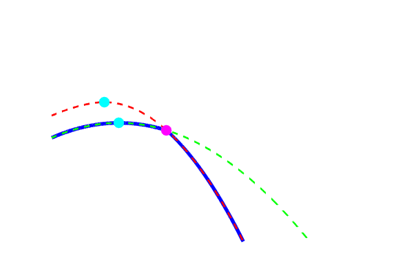
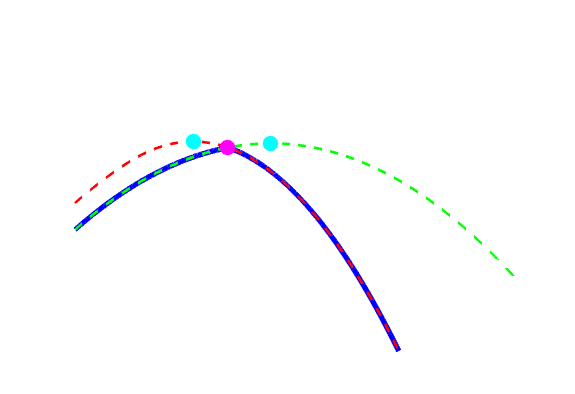
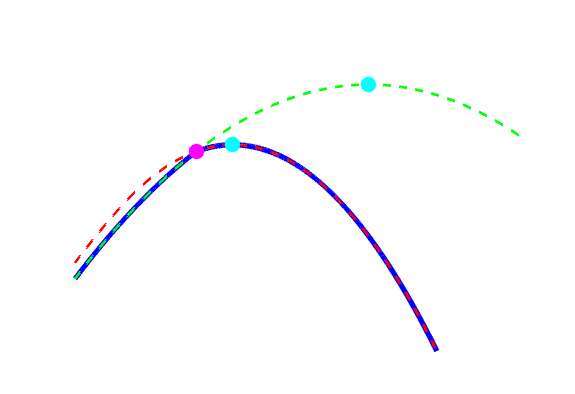
Figure 6: Illustration of the three different cases for the proximal operator.

3.2 Modifying Algorithm 1

Following the approach used in [18], consider the program

$$\max_{s} \min\{b_{i},[s-a_{i}]_{+}^{2}\}-\frac{\rho+1}{\rho}(s-\sigma_{i}(Y))^{2}$$ (53)

$$+s^{2}-[s-a_{i}]_{+}^{2},$$

s.t. $$\sigma_{i+1}(Z)\leq s\leq\sigma_{i-1}(Z).$$

Note that the objective function is the pointwise minimum of

$$f_{1}(s) =b_{i}-\frac{\rho+1}{\rho}(s-\sigma_{i}(Y))^{2}+s^{2}-[s-a_{i}]_{+}^{2},$$ (54)

$$f_{2}(s) =s^{2}-\frac{\rho+1}{\rho}(s-\sigma_{i}(Y))^{2},$$

both of which are concave, since $\frac{\rho+1}{\rho}>1$. For $f_{1}$ the maximum is obtained in $s=\frac{a_{i}\rho}{\rho+1}+\sigma_{i}(Y)$, if $s\geq a_{i}$ otherwise when $s=(\rho+1)\sigma_{i}(Y)$. The minimum of $f_{2}$ is obtained when $s=(\rho+1)\sigma_{i}(Y)$.

There are three possible cases, also shown in Figure 6.

1. The maximum occurs when $s>a_{i}+\sqrt{b_{i}}$, hence $f_{1}(s)<f_{2}(s)$, hence $s=\frac{a_{i}\rho}{\rho+1}+\sigma_{i}(Y)$.

2. The maximum occurs when $s<a_{i}+\sqrt{b_{i}}$, where $f_{1}(s)>f_{2}(s)$, hence $s=(\rho+1)\sigma_{i}(Y)$.

3. When $s=a_{i}+\sqrt{b_{i}}$, which is valid elsewhere.

in summary

$$s_{i}=\left\{\begin{aligned} &\frac{a_{i}\rho}{\rho+1}+\sigma_{i}(Y),&&\frac{a_{i}}{\rho+1}+\sqrt{b_{i}}<\sigma_{i}(Y),\\ &a_{i}+\sqrt{b_{i}},&&\frac{a_{i}+\sqrt{b_{i}}}{1+\rho}\leq\sigma_{i}(Y)\leq\frac{a_{i}}{\rho+1}+\sqrt{b_{i}},\\ &(1+\rho)\sigma_{i}(Y),&&\sigma_{i}(Y)<\frac{a_{i}+\sqrt{b_{i}}}{1+\rho},\end{aligned}\right.$$ (55)

By replacing the sequence of unconstrained minimizers $\{s_{i}\}$ defined by (55), with the corresponding sequence in Section 4 (of the main paper), and changing the objective function of Algorithm 1, to the one in (53), the maximizing singular value vector fo the proximal operator is obtained.

References

- [1] Roland Angst, Christopher Zach, and Marc Pollefeys. The generalized trace-norm and its application to structure-from-motion problems. In International Conference on Computer Vision, 2011.
- [2] Ronen Basri, David Jacobs, and Ira Kemelmacher. Photometric stereo with general, unknown lighting. International Journal of Computer Vision, 72(3):239–257, May 2007.
- [3] Stephen Boyd, Neal Parikh, Eric Chu, Borja Peleato, and Jonathan Eckstein. Distributed optimization and statistical learning via the alternating direction method of multipliers. Found. Trends Mach. Learn., 3(1):1–122, 2011.
- [4] C. Bregler, A. Hertzmann, and H. Biermann. Recovering non-rigid 3d shape from image streams. In The IEEE Conference on Computer Vision and Pattern Recognition (CVPR), 2000.
- [5] R. Cabral, F. De la Torre, J. P. Costeira, and A. Bernardino. Unifying nuclear norm and bilinear factorization approaches for low-rank matrix decomposition. In International Conference on Computer Vision (ICCV), 2013.
- [6] Emmanuel J Candès, Xiaodong Li, Yi Ma, and John Wright. Robust principal component analysis? Journal of the ACM (JACM), 58(3):11, 2011.
- [7] Emmanuel J. Candès, Xiaodong Li, Yi Ma, and John Wright. Robust principal component analysis? J. ACM, 58(3):11:1–11:37, 2011.
- [8] Emmanuel J Candes, Michael B Wakin, and Stephen P Boyd. Enhancing sparsity by reweighted minimization. Journal of Fourier analysis and applications, 14(5-6):877–905, 2008.
- [9] Lu Canyi, Jinhui Tang, Shuicheng Yan, and Zhouchen Lin. Nonconvex nonsmooth low-rank minimization via iteratively reweighted nuclear norm. IEEE Transactions on Image Processing, 25, 10 2015.
- [10] Marcus Carlsson. On convexification/optimization of functionals including an l2-misfit term. arXiv preprint arXiv:1609.09378, 2016.
- [11] Yuchao Dai, Hongdong Li, and Mingyi He. A simple prior-free method for non-rigid structure-from-motion factorization. International Journal of Computer Vision, 107(2):101–122, 2014.
- [12] Ravi Garg, Anastasios Roussos, and Lourdes Agapito. A variational approach to video registration with subspace constraints. International Journal of Computer Vision, 104(3):286–314, 2013.
- [13] N. Gillis and F. Glinuer. Low-rank matrix approximation with weights or missing data is np-hard. SIAM Journal on Matrix Analysis and Applications, 32(4), 2011.
- [14] Shuhang Gu, Qi Xie, Deyu Meng, Wangmeng Zuo, Xiangchu Feng, and Lei Zhang. Weighted nuclear norm minimization and its applications to low level vision. International Journal of Computer Vision, 121, 07 2016.
- [15] Y. Hu, D. Zhang, J. Ye, X. Li, and X. He. Fast and accurate matrix completion via truncated nuclear norm regularization. IEEE Transactions on Pattern Analysis and Machine Intelligence, 35(9):2117–2130, 2013.
- [16] Suryansh Kumar. A simple prior-free method for non-rigid structure-from-motion factorization : Revisited. CoRR, abs/1902.10274, 2019.
- [17] Viktor Larsson, Erik Bylow, Carl Olsson, and Fredrik Kahl. Rank minimization with structured data patterns. In European Conference on Computer Vision, 2014.
- [18] Viktor Larsson and Carl Olsson. Convex low rank approximation. International Journal of Computer Vision, 120(2):194–214, 2016.
- [19] Viktor Larsson and Carl Olsson. Compact matrix factorization with dependent subspaces. In The IEEE Conference on Computer Vision and Pattern Recognition (CVPR), pages 4361–4370, 07 2017.
- [20] Karthik Mohan and Maryam Fazel. Iterative reweighted least squares for matrix rank minimization. In Annual Allerton Conference on Communication, Control, and Computing, pages 653–661, 2010.
- [21] R. A. Newcombe, D. Fox, and S. M. Seitz. Dynamicfusion: Reconstruction and tracking of non-rigid scenes in real-time. In Conference on Computer Vision and Pattern Recognition (CVPR), pages 343–352, June 2015.
- [22] Feiping Nie, Hua Wang, Xiao Cai, Heng Huang, and Chris H. Q. Ding. Robust matrix completion via joint schatten p-norm and lp-norm minimization. In ICDM, pages 566–574, 2012.
- [23] T. H. Oh, Y. W. Tai, J. C. Bazin, H. Kim, and I. S. Kweon. Partial sum minimization of singular values in robust pca: Algorithm and applications. IEEE Transactions on Pattern Analysis and Machine Intelligence, 38(4):744–758, 2016.
- [24] Carl Olsson, Marcus Carlsson, Fredrik Andersson, and Viktor Larsson. Non-convex rank/sparsity regularization and local minima. Proceedings of the International Conference on Computer Vision, 2017.
- [25] S. Oymak, A. Jalali, M. Fazel, Y. C. Eldar, and B. Hassibi. Simultaneously structured models with application to sparse and low-rank matrices. IEEE Transactions on Information Theory, 61(5):2886–2908, 2015.
- [26] Benjamin Recht, Maryam Fazel, and Pablo A. Parrilo. Guaranteed minimum-rank solutions of linear matrix equations via nuclear norm minimization. SIAM Rev., 52(3):471–501, Aug. 2010.
- [27] C. Russell, R. Yu, and L. Agapito. Video-popup: Monocular 3d reconstruction of dynamic scenes. In European Conference on Computer Vision (ECCV), 2014.
- [28] F. Shang, J. Cheng, Y. Liu, Z. Luo, and Z. Lin. Bilinear factor matrix norm minimization for robust pca: Algorithms and applications. IEEE Transactions on Pattern Analysis and Machine Intelligence, 40(9):2066–2080, Sep. 2018.
- [29] Kim-Chuan Toh and Sangwoon Yun. An accelerated proximal gradient algorithm for nuclear norm regularized least squares problems. Pacific Journal of Optimization, 6, 09 2010.
- [30] J. Valmadre, S. Sridharan, S. Denman, C. Fookes, and S. Lucey. Closed-form solutions for low-rank non-rigid reconstruction. In 2015 International Conference on Digital Image Computing: Techniques and Applications (DICTA), pages 1–6, Nov 2015.
- [31] Jun Xu, Lei Zhang, David Zhang, and Xiangchu Feng. Multi-channel weighted nuclear norm minimization for real color image denoising. International Conference on Computer Vision (ICCV), 2017.
- [32] Noam Yair and Tomer Michaeli. Multi-scale weighted nuclear norm image restoration. In Conference on Computer Vision and Pattern Recognition (CVPR), 2018.