Backreacting holographic superconductors from the coupling of a scalar field to the Einstein tensor

Abstract

Abstract

We investigate the properties of the backreacting holographic superconductors from the coupling of a scalar field to the Einstein tensor in the background of a $d$-dimensional AdS black hole. Imposing the Dirichlet boundary condition of the trial function without the Neumann boundary conditions, we improve the analytical Sturm-Liouville method with an iterative procedure to explore the pure effect of the Einstein tensor on the holographic superconductors and find that the Einstein tensor hinders the condensate of the scalar field but does not affect the critical phenomena. Our analytical findings are in very good agreement with the numerical results from the “marginally stable modes” method, which implies that the Sturm-Liouville method is still powerful to study the holographic superconductors from the coupling of a scalar field to the Einstein tensor even if we consider the backreactions.

I Introduction

It is well known that the superconductivity is one of the most remarkable phenomena observed in physics in the 20th century Tinkham . However, the core mechanism of the high-temperature superconductor systems, which can not be described by the usual Bardeen-Cooper-Schrieffer (BCS) theory BCS , is still one of the unsolved mysteries in theoretical physics so far. Interestingly, it was suggested that it is logical to investigate the properties of high temperature superconductors on the boundary of spacetime by considering the classical general relativity in one higher dimension with the help of the Anti-de Sitter/conformal field theories (AdS/CFT) correspondence Maldacena ; Gubser1998 ; Witten . In the probe limit, Gubser observed that the spontaneous $U(1)$ symmetry breaking by bulk black holes can be used to construct gravitational dual of the transition from normal state to superconducting state GubserPRD78 , and Hartnoll et al. found that the properties of a ($2+1$)-dimensional superconductor can indeed be reproduced in the ($3+1$)-dimensional holographic dual model based on the framework of usual Maxwell electrodynamics HartnollPRL101 . Extending the investigation to the so-called holographic superconductor models away from the probe limit, i.e., taking the backreactions of the spacetime into account, the authors of Ref. HartnollJHEP12 showed that even the uncharged scalar field can form a condensate in the $(2+1)$-dimensional holographic superconductor model. Along this line, there has been accumulated interest in studying the effects of the backreaction on the holographic $s$-wave PanJWCh ; BarclayGregory ; Barclay2011 ; GregoryRev ; KannoCQG ; Ge2011 ; Herzog2010 ; Gubser-Nellore ; Horowitz-Way ; Aprile-Russo ; Brihaye ; Liu-Sun ; Siani ; PanWangBR ; LiuWangBTZ ; LPW2012 ; GangopadhyayPLB ; LiuGongWang ; YaoJing ; EmparanTanabe ; DeyJHEP2014 ; NakoniecznyRogatko ; MomeniPLB2015 ; Ghorai2016 ; JingCQG ; SheykhiShakerPLB ; Peng2017 ; SheykhiShakerIJMPD ; SherkatghanadIJMPD ; YaoJing2018 ; Ghotbabadi2018 ; GhoraiNPB2018 ; MohammadiSZ2018 $p$-wave CaiNieZhang2011 ; AriasLandea ; CaiPWave-1 ; CaiPWave-2 ; CSJHEP2015 ; NieCai2015 ; Wang2016 ; Nie2017 and $d$-wave GTWjhep2012 dual models. Reviews of the holographic superconductors can be found in Refs. HartnollRev ; HerzogRev ; HorowitzRev ; CaiRev .

Most of the aforementioned works on the gravitational dual models focus on the superconductors without an impurity. As a matter of fact, to study the effect of impurities is often important since their presence can drastically change the physical properties of the superconductors in condensed matter physics Balatsky . According to the AdS/CFT duality, Ishii and Sin investigated the impurity effect in a holographic superconductor by turning on a coupling between the gauge field and a new massive gauge field, and found that the mass gap in the optical conductivity disappears when the coupling is sufficiently large Ishii . Zeng and Zhang studied the single normal impurity effect in a superconductor by using the holographic approach, which showed that the critical temperature of the host superconductor decreases as the size of the impurity increases and the phase transition at the critical impurity strength (or the critical temperature) is of zeroth order ZengZhang . Fang et al. extended the study to the Fermionic phase transition induced by the effective impurity in holography and obtained a phase diagram in $(\alpha,T)$ plane separating the Fermi liquid phase and the non-Fermi liquid phase FangJHEP . More recently, Kuang and Papantonopoulos built a holographic superconductor with a scalar field coupled kinematically to the Einstein tensor and observed that, as the strength of the coupling increases, the critical temperature below which the scalar field condenses is lowering, the condensation gap decreases faster than the temperature, the width of the condensation gap is not proportional to the size of the condensate and at low temperatures the condensation gap tends to zero for the strong coupling KuangE2016 . Obviously, these effects suggest that the derivative coupling in the gravity bulk can have a dual interpretation on the boundary corresponding to impurities concentrations in a real material. Note that they concentrated on the probe limit where the backreaction of matter fields on the spacetime metric is neglected. Thus, in this work we will extend their interesting model to the case away from the probe limit and explore the effect of the Einstein tensor on the holographic superconductors with backreactions. In addition, we will compare the result in five dimensions with that in four dimensions and present an analysis of the effect the extra dimension has on the scalar condensation formation. In the calculation, we first use the Sturm-Liouville eigenvalue problem Siopsis ; SiopsisBF to analytically study the holographic superconductor phase transition, and then count on the “marginally stable modes” method GubserPRD78 ; marginally stable modes to numerically confirm the analytical findings and verify the effectiveness of the Sturm-Liouville method.

The organization of the work is as follows. In Sec. II, we will introduce the backreacting holographic superconductor models from the coupling of a scalar field to the Einstein tensor in the $d$-dimensional AdS black hole background. In Sec. III we will give an analytical investigation of the holographic superconductors by using the Sturm-Liouville method. In Sec. IV we will give a numerical investigation of the holographic superconductors by using the “marginally stable modes” method. We will summarize our results in the last section.

II Description of the holographic dual system

The general action describing a charged, complex scalar field coupled to the Einstein tensor $G^{\mu\nu}$ in the $d$-dimensional Einstein-Maxwell action with negative cosmological constant $\Lambda=-(d-1)(d-2)/(2L^{2})$ is of the form

$$S=\int d^{d}x\sqrt{-g}\left[\frac{1}{2\kappa^{2}}\left(R-2\Lambda\right)-\frac{1}{4}F_{\mu\nu}F^{\mu\nu}-(g^{\mu\nu}+\eta G^{\mu\nu})D_{\mu}\psi(D_{\nu}\psi)^{\ast}-m^{2}|\psi|^{2}\right],$$ (1)

with $D_{\mu}=\nabla_{\mu}-iqA_{\mu}$. Here $\kappa^{2}=8\pi G_{d}$ represents the gravitational constant, $F_{\mu\nu}=\nabla_{\mu}A_{\nu}-\nabla_{\nu}A_{\mu}$ is the Maxwell field strength, and $\psi$ denotes the scalar field with the charge $q$ and mass $m$. When the coupling parameter $\eta\rightarrow 0$, our model reduces to the standard holographic superconductors with backreactions investigated in HartnollJHEP12 ; PanJWCh . It should be noted that we can rescale the bulk fields $\psi$ and $A_{\mu}$ as $\psi/q$ and $A_{\mu}/q$ in order to put the factor $1/q^{2}$ as the backreaction parameter for the matter fields. So the probe limit can be obtained safely if $\kappa^{2}/q^{2}\rightarrow 0$. Without loss of generality, we can set $q=1$ and keep $\kappa^{2}$ finite when we take the backreaction into account, just as in Refs. PanJWCh ; BarclayGregory ; Barclay2011 ; GregoryRev ; KannoCQG ; CSJHEP2015 .

To go beyond the probe limit, we adopt the metric ansatz for the black hole with the curvature $k=0$ as

$$ds^{2}=-f(r)e^{-\chi(r)}dt^{2}+\frac{dr^{2}}{f(r)}+r^{2}h_{ij}dx^{i}dx^{j},$$ (2)

where $f$ and $\chi$ are functions of $r$ only, $h_{ij}dx^{i}dx^{j}$ represents the line element of a ($d-2$)-dimensional hypersurface. Obviously, the Hawking temperature of this $d$-dimensional black hole, which will be interpreted as the temperature of the CFT, can be given by

$$T_{H}=\frac{f^{\prime}(r_{+})e^{-\chi(r_{+})/2}}{4\pi},$$ (3)

where the prime denotes a derivative with respect to $r$, and the black hole horizon $r_{+}$ is determined by $f(r_{+})=0$. For the considered ansatz (2), the nonzero components of the Einstein tensor $G^{\mu\nu}$ are

$$G^{tt}=-\frac{(d-2)e^{\chi}}{2r^{2}}\left[(d-3)+\frac{rf^{\prime}}{f}\right],~{}~{}G^{rr}=\frac{(d-2)f^{2}}{2r^{2}}\left[(d-3)+\frac{rf^{\prime}}{f}-r\chi^{\prime}\right],$$

$$G^{xx}=G^{yy}=\cdot\cdot\cdot=\frac{1}{4r^{3}}\left\{f^{\prime}\left[4(d-3)-3r\chi^{\prime}\right]+2rf^{\prime\prime}+f\left[\frac{2(d-3)(d-4)}{r}-2(d-3)\chi^{\prime}+r\chi^{\prime 2}-2r\chi^{\prime\prime}\right]\right\}.$$

For the scalar field and electromagnetic field, we will take $\psi=|\psi|$, $A_{t}=\phi$ where $\psi$, $\phi$ are both real functions of $r$ only. Thus, from the action (1) we can give the equations of motion for the metric functions $f(r)$ and $\chi(r)$

$$\bigg{[}1+\eta\kappa^{2}\bigg{(}\frac{e^{\chi}\phi^{2}\psi^{2}}{f}-3f\psi^{\prime 2}\bigg{)}\bigg{]}\chi^{\prime} +$$

$$\frac{4\kappa^{2}r}{d-2}\bigg{\{}\psi^{\prime 2}+\frac{e^{\chi}\phi^{2}\psi^{2}}{f^{2}}+\frac{(d-2)\eta}{2r}\bigg{[}\frac{(d-3)f}{r}\left(\psi^{\prime 2}+\frac{e^{\chi}\phi^{2}\psi^{2}}{f^{2}}\right)+\frac{2e^{\chi}\phi\psi(\phi\psi)^{\prime}}{f}-2f\psi^{\prime}\psi^{\prime\prime}\bigg{]}\bigg{\}} = 0,$$ (5)

$$\bigg{[}1+\eta\kappa^{2}\left(\frac{e^{\chi}\phi^{2}\psi^{2}}{f}-3f\psi^{\prime 2}\right)\bigg{]}f^{\prime}-\left[\frac{(d-1)r}{L^{2}}-\frac{(d-3)f}{r}\right]+\frac{2\kappa^{2}r}{d-2}\bigg{\{}m^{2}\psi^{2}+\frac{e^{\chi}\phi^{\prime 2}}{2} +$$

$$f\bigg{(}\psi^{\prime 2}+\frac{e^{\chi}\phi^{2}\psi^{2}}{f^{2}}\bigg{)}+\frac{(d-2)\eta}{2r}\bigg{[}\frac{(d-3)e^{\chi}\phi^{2}\psi^{2}}{r}-\frac{(d-3)f^{2}\psi^{\prime 2}}{r}-4f^{2}\psi^{\prime}\psi^{\prime\prime}\bigg{]}\bigg{\}} = 0,$$ (6)

and for the matter fields $\phi(r)$ and $\psi(r)$

$$\phi^{\prime\prime}+\left(\frac{d-2}{r}+\frac{\chi^{\prime}}{2}\right)\phi^{\prime}-\frac{2\psi^{2}}{f}\left[1+\frac{(d-2)\eta f}{2r}\bigg{(}\frac{d-3}{r}+\frac{f^{\prime}}{f}\bigg{)}\right]\phi=0,$$ (7)

$$\left\{1+\frac{(d-2)\eta}{2r}\bigg{[}\frac{(d-3)f}{r}+f^{\prime}-f\chi^{\prime}\bigg{]}\right\}\psi^{\prime\prime}+\bigg{\{}\left(\frac{d-2}{r}+\frac{f^{\prime}}{f}-\frac{\chi^{\prime}}{2}\right) +$$

$$\frac{(d-2)\eta}{2r}\bigg{[}f^{\prime\prime}+\frac{3(d-3)f^{\prime}}{r}+\frac{f^{\prime 2}}{f}+\frac{f\chi^{\prime 2}}{2}-\frac{3(d-3)f\chi^{\prime}}{2r}-\frac{5f^{\prime}\chi^{\prime}}{2}-f\chi^{\prime\prime}+\frac{(d-3)(d-4)f}{r^{2}}\bigg{]}\bigg{\}}\psi^{\prime} +$$

$$\left\{\frac{e^{\chi}\phi^{2}}{f^{2}}\bigg{[}1+\frac{(d-2)(d-3)\eta f}{2r^{2}}+\frac{(d-2)\eta f^{\prime}}{2r}\bigg{]}-\frac{m^{2}}{f}\right\}\psi = 0,$$ (8)

where the prime denotes a derivative with respect to $r$.

We will count on the appropriate boundary conditions to get the solutions in the superconducting phase, $\psi(r)\neq 0$. At the horizon $r=r_{+}$ of the black hole, the regularity gives the boundary conditions

$$\phi(r_{+})=0\,,\hskip 14.22636pt\psi(r_{+})=\frac{1}{m^{2}}\left[f^{\prime}(r_{+})+\frac{(d-2)\eta f^{\prime}(r_{+})^{2}}{2r_{+}}\right]\psi^{\prime}(r_{+}),$$

$$\chi^{\prime}(r_{+})=-\frac{4\kappa^{2}r_{+}}{d-2}\bigg{[}\psi^{\prime}(r_{+})^{2}+\frac{e^{\chi(r_{+})}\phi^{\prime}(r_{+})^{2}\psi(r_{+})^{2}}{f^{\prime}(r_{+})^{2}}+\frac{(d-2)\eta e^{\chi(r_{+})}\phi^{\prime}(r_{+})^{2}\psi(r_{+})^{2}}{r_{+}f^{\prime}(r_{+})}\bigg{]},$$

$$f^{\prime}(r_{+})=\frac{(d-1)r_{+}}{L^{2}}-\frac{2\kappa^{2}r_{+}}{d-2}\left[m^{2}\psi(r_{+})^{2}+\frac{1}{2}e^{\chi(r_{+})}\phi^{\prime}(r_{+})^{2}\right].$$ (9)

At the asymptotic boundary $r\rightarrow\infty$, the solutions behave like

$$\chi\rightarrow 0\,,\hskip 14.22636ptf\sim\frac{r^{2}}{L^{2}}\,,\hskip 14.22636pt\phi\sim\mu-\frac{\rho}{r^{d-3}}\,,\hskip 14.22636pt\psi\sim\frac{\psi_{-}}{r^{\Delta_{-}}}+\frac{\psi_{+}}{r^{\Delta_{+}}}\,,$$ (10)

with the characteristic exponent

$$\Delta_{\pm}=\frac{1}{2}\left[(d-1)\pm\sqrt{(d-1)^{2}+\frac{8m^{2}L^{2}}{2+(d-1)(d-2)\eta}}~{}\right].$$ (11)

According to the AdS/CFT correspondence, $\mu$ and $\rho$ are interpreted as the chemical potential and charge density in the dual field theory, respectively. Considering the stability of the scalar field, we find that the mass should be above the Breitenlohner-Freedman (BF) bound $m^{2}_{BF}=-(d-1)^{2}[2+(d-1)(d-2)\eta]/(8L^{2})$ Breitenloher , which depends on the coupling parameter $\eta$ and dimensionality of the AdS space $d$. Note that, provided $\Delta_{-}$ is larger than the unitarity bound, both $\psi_{-}$ and $\psi_{+}$ can be normalizable and be used to define operators on the dual field theory, $\psi_{-}=\langle{\cal O}_{-}\rangle$, $\psi_{+}=\langle{\cal O}_{+}\rangle$, respectively HartnollPRL101 ; HartnollJHEP12 . In this work, we impose boundary condition $\psi_{-}=0$ since we concentrate on the condensate for the operator $\langle{\cal O}_{+}\rangle$.

In the normal phase, $\psi(r)=0$, the metric coefficient $\chi$ is a constant from Eq. (II) and the analytical solutions to Eqs. (II) and (7) lead to the Reissner-Nordström AdS black holes

$$f=\frac{r^{2}}{L^{2}}-\frac{1}{r^{d-3}}\left[\frac{r^{d-1}_{+}}{L^{2}}+\frac{(d-3)\kappa^{2}\rho^{2}}{(d-2)r^{d-3}_{+}}\right]+\frac{(d-3)\kappa^{2}\rho^{2}}{(d-2)r^{2(d-3)}}\,,\hskip 14.22636pt\phi=\mu-\frac{\rho}{r^{d-3}},$$ (12)

where the metric coefficient $f$ goes back to the case of the Schwarzschild AdS black hole when $\kappa=0$.

On the other hand, from the equations of motion (II)-(8) we can obtain the useful scaling symmetries and the transformation of the relevant quantities

$$r\rightarrow\alpha r,~{}~{}(t,x^{i})\rightarrow\frac{1}{\alpha}(t,x^{i}),$$

$$(\chi,\psi,L)\rightarrow(\chi,\psi,L),~{}~{}(\phi,\mu,T)\rightarrow\alpha(\phi,\mu,T),$$

$$\rho\rightarrow\alpha^{d-2}\rho,~{}~{}\psi_{\pm}\rightarrow\alpha^{\Delta_{\pm}}\psi_{\pm},$$ (13)

where $\alpha$ is a real positive number. For simplicity, we use the scaling symmetries to set $L=1$ when performing calculations in the following sections.

III Critical behavior from the Sturm-Liouville method

We use the variational method for the Sturm-Liouville eigenvalue problem Siopsis ; SiopsisBF to analytically investigate the properties of the backreacting holographic superconductors from the coupling of a scalar field to the Einstein tensor. We will derive the critical behavior of the system near the phase transition point and examine the effects of the Einstein tensor and backreaction on the holographic superconductors.

For convenience, we introduce a new variable $z=r_{+}/r$ and rewrite the equations of motion (II)-(8) into

$$\bigg{[}1+\eta\kappa^{2}\bigg{(}\frac{e^{\chi}\phi^{2}\psi^{2}}{f}-\frac{3z^{4}f\psi^{\prime 2}}{r_{+}^{2}}\bigg{)}\bigg{]}\chi^{\prime}-\frac{4\kappa^{2}}{d-2}\bigg{\{}z\psi^{\prime 2}+\frac{r_{+}^{2}e^{\chi}\phi^{2}\psi^{2}}{z^{3}f^{2}} +$$

$$\frac{(d-2)\eta}{2}\bigg{[}\frac{(d-3)e^{\chi}\phi^{2}\psi^{2}}{zf}-\frac{2e^{\chi}\phi\psi(\phi\psi)^{\prime}}{f}+\frac{(d+1)z^{3}f\psi^{\prime 2}}{r_{+}^{2}}+\frac{2z^{4}f\psi^{\prime}\psi^{\prime\prime}}{r_{+}^{2}}\bigg{]}\bigg{\}} = 0,$$ (14)

$$\bigg{[}1+\eta\kappa^{2}\bigg{(}\frac{\phi^{2}\psi^{2}e^{\chi}}{f}-\frac{3z^{4}f\psi^{\prime 2}}{r_{+}^{2}}\bigg{)}\bigg{]}f^{\prime}-\frac{(d-3)f}{z}+\frac{(d-1)r^{2}_{+}}{z^{3}}-\frac{2r_{+}^{2}\kappa^{2}}{(d-2)z^{3}}\bigg{\{}m^{2}\psi^{2}+\frac{e^{\chi}z^{4}\phi^{\prime 2}}{2r_{+}^{2}} +$$

$$f\bigg{(}\frac{e^{\chi}\phi^{2}\psi^{2}}{f^{2}}+\frac{z^{4}\psi^{\prime 2}}{r_{+}^{2}}\bigg{)}+\frac{(d-2)\eta}{2r_{+}^{2}}\bigg{[}(d-3)z^{2}\phi^{2}\psi^{2}e^{\chi}-\frac{(d-11)z^{6}f^{2}\psi^{\prime 2}}{r_{+}^{2}}+\frac{4z^{7}f^{2}\psi^{\prime}\psi^{\prime\prime}}{r_{+}^{2}}\bigg{]}\bigg{\}} = 0,$$ (15)

$$\phi^{\prime\prime}+\left(\frac{\chi^{\prime}}{2}-\frac{d-4}{z}\right)\phi^{\prime}-\frac{2r_{+}^{2}\psi^{2}}{z^{4}f}\bigg{[}1+\frac{(d-2)\eta z^{2}f}{2r_{+}^{2}}\bigg{(}d-3-\frac{zf^{\prime}}{f}\bigg{)}\bigg{]}\phi=0,$$ (16)

$$\bigg{[}1+\frac{(d-2)\eta z^{2}f}{2r_{+}^{2}}\bigg{(}d-3+z\chi^{\prime}-\frac{zf^{\prime}}{f}\bigg{)}\bigg{]}\psi^{\prime\prime}-\bigg{\{}\frac{\chi^{\prime}}{2}+\frac{d-4}{z}-\frac{f^{\prime}}{f}+\frac{(d-2)\eta}{2r_{+}^{2}}\bigg{[}(d-3)(d-6)zf +$$

$$\frac{z^{3}f^{\prime 2}}{f}-(3d-13)z^{2}f^{\prime}+z^{3}f^{\prime\prime}+\frac{z^{3}f\chi^{\prime 2}}{2}-\frac{5z^{3}f^{\prime}\chi^{\prime}}{2}+\frac{(3d-17)z^{2}f\chi^{\prime}}{2}-z^{3}f\chi^{\prime\prime}\bigg{]}\bigg{\}}\psi^{\prime} +$$

$$\frac{r_{+}^{2}e^{\chi}\phi^{2}}{z^{4}f^{2}}\bigg{[}1+\frac{(d-2)\eta z^{2}f}{2r_{+}^{2}}\bigg{(}d-3-\frac{zf^{\prime}}{f}\bigg{)}\bigg{]}\psi-\frac{m^{2}r_{+}^{2}}{z^{4}f}\psi = 0,$$ (17)

where the prime now denotes the derivative with respect to $z$. Note that the scalar field $\psi=0$ at the critical temperature $T_{c}$. Therefore the expectation value of the scalar operator $\langle{\cal O}_{+}\rangle$ is small near the critical point and we can select it as an expansion parameter $\epsilon\equiv\langle{\cal O}_{+}\rangle$ with $\epsilon\ll 1$. Since we are interested in solutions where $\psi$ is small, so from Eqs. (16) and (III) we can expand the scalar field $\psi(z)$ and the gauge field $\phi(z)$ as PanJWCh ; KannoCQG ; Ge2011 ; Herzog2010

$$\psi=\epsilon\psi_{1}+\epsilon^{3}\psi_{3}+\epsilon^{5}\psi_{5}+\cdot\cdot\cdot,$$

$$\phi=\phi_{0}+\epsilon^{2}\phi_{2}+\epsilon^{4}\phi_{4}+\cdot\cdot\cdot,$$ (18)

and from Eqs. (14) and (III) the metric functions $f(z)$ and $\chi(z)$ can be expanded around the Reissner-Nordström AdS spacetime as

$$f=f_{0}+\epsilon^{2}f_{2}+\epsilon^{4}f_{4}+\cdot\cdot\cdot,$$

$$\chi=\epsilon^{2}\chi_{2}+\epsilon^{4}\chi_{4}+\cdot\cdot\cdot.$$ (19)

Considering that the chemical potential $\mu$ can be corrected order by order $\mu=\mu_{0}+\epsilon^{2}\delta\mu_{2}+\cdot\cdot\cdot$ with $\delta\mu_{2}>0$ Herzog2010 , we get a result for the order parameter as a function of the chemical potential near the phase transition

$$\epsilon\equiv\langle{\cal O}_{+}\rangle\approx\left(\frac{\mu-\mu_{0}}{\delta\mu_{2}}\right)^{1/2},$$ (20)

which indicates that the holographic s-wave superconducting phase transition with backreaction from the coupling of a scalar field to the Einstein tensor is of the second order and the critical exponent of the system always takes the mean-field value 1/2. The Einstein tensor, backreaction and spacetime dimension will not influence the result. When $\mu\rightarrow\mu_{0}$, the phase transition occurs and the order parameter is zero at the critical point, which means that the critical value $\mu$ is $\mu_{c}=\mu_{0}$.

Now we are in a position to solve equations order by order. At the zeroth order, the equation of motion for the Maxwell field (16) reduces to

$$\phi_{0}^{\prime\prime}(z)-\frac{d-4}{z}\phi_{0}^{\prime}(z)=0,$$ (21)

which has a solution $\phi_{0}(z)=\mu_{0}(1-z^{d-3})$ with $\mu_{0}=\rho/r^{d-3}_{+}$. Since $\mu_{0}=\mu_{c}=\rho/r^{d-3}_{+c}$ at the critical point $\mu_{c}$, where $r_{+c}$ is the radius of the horizon at the critical point, we will have

$$\phi_{0}(z)=\lambda r_{+c}(1-z^{d-3}),$$ (22)

where we have set a dimensionless quantity $\lambda=\rho/r^{d-2}_{+c}$. Inserting this solution into Eq. (III), we can give the equation of motion for the metric function $f_{0}(z)$, i.e.,

$$f_{0}^{\prime}-\frac{(d-3)f_{0}}{z}+\frac{(d-1)r^{2}_{+}}{z^{3}}-\frac{\kappa^{2}z\phi_{0}^{\prime 2}}{d-2}=0,$$ (23)

with its solution

$$f_{0}(z)=r^{2}_{+}\xi(z)=r^{2}_{+}\left[\frac{1}{z^{2}}-z^{d-3}-\frac{(d-3)\kappa^{2}\lambda^{2}}{d-2}z^{d-3}(1-z^{d-3})\right],$$ (24)

where we have defined a new function $\xi(z)$ for simplicity.

At the first order, the equation of motion for $\psi_{1}(z)$ is

$$\bigg{[}1+\frac{(d-2)\eta z^{2}f_{0}}{2r_{+}^{2}}\bigg{(}d-3-\frac{zf_{0}^{\prime}}{f_{0}}\bigg{)}\bigg{]}\psi_{1}^{\prime\prime}-\bigg{\{}\frac{d-4}{z}-\frac{f_{0}^{\prime}}{f_{0}}+\frac{(d-2)\eta}{2r_{+}^{2}}\bigg{[}(d-3)(d-6)zf_{0}+\frac{z^{3}f_{0}^{\prime 2}}{f_{0}} -$$

$$(3d-13)z^{2}f_{0}^{\prime}+z^{3}f_{0}^{\prime\prime}\bigg{]}\bigg{\}}\psi_{1}^{\prime}+\frac{r_{+}^{2}\phi_{0}^{2}}{z^{4}f_{0}^{2}}\bigg{[}1+\frac{(d-2)\eta z^{2}f_{0}}{2r_{+}^{2}}\bigg{(}d-3-\frac{zf_{0}^{\prime}}{f_{0}}\bigg{)}\bigg{]}\psi_{1}-\frac{m^{2}r_{+}^{2}}{z^{4}f_{0}}\psi_{1} = 0,$$ (25)

which has the asymptotic AdS boundary condition $\psi_{1}\sim\frac{\psi_{-}}{r_{+}^{\Delta_{-}}}z^{\Delta_{-}}+\frac{\psi_{+}}{r_{+}^{\Delta_{+}}}z^{\Delta_{+}}$. Just as in the interesting works by Kolyvaris et al. KolyvarisKPSA ; KolyvarisKPSB , we will use Eq. (25) to discuss the stability of our solutions. We can express the effective potential of $\psi_{1}$ as

$$V_{eff,0}(z)=-\frac{f^{2}_{0}}{r_{+}^{4}}\left\{\frac{z^{4}P^{\prime\prime}(z)}{P(z)}-\frac{r_{+}^{d-2}W(z)P(z)P^{\prime}(z)}{z^{d-5}}-\frac{r_{+}^{d}P^{2}(z)}{z^{d-2}f_{0}}\left[m^{2}-\frac{z^{d-2}\phi^{2}_{0}}{r_{+}^{d-2}f_{0}P^{2}(z)}\right]\right\},$$ (26)

with the defined functions

$$P(z) = \left(\frac{z}{r_{+}}\right)^{\frac{d-2}{2}}\bigg{[}1+\frac{(d-2)\eta z^{2}f_{0}}{2r_{+}^{2}}\bigg{(}d-3-\frac{zf_{0}^{\prime}}{f_{0}}\bigg{)}\bigg{]}^{-\frac{1}{2}},$$

$$W(z) = (d-4)-\frac{zf^{\prime}_{0}}{f_{0}}+\frac{(d-2)\eta z^{2}}{2r_{+}^{2}}\bigg{[}(d-3)(d-6)f_{0}+\frac{z^{2}f_{0}^{\prime 2}}{f_{0}}-(3d-13)zf_{0}^{\prime}+z^{2}f_{0}^{\prime\prime}\bigg{]},$$ (27)

which can develop a negative gap near the black hole horizon, implying a potential instability of the black hole. In Fig. 1, we plot the curves of the effective potential $V_{eff,0}(z)$ with different values of the coupling parameter $\eta$ for the fixed mass of the scalar field $m^{2}=-3$ (top-left) and $m^{2}=0$ (top-right), backreaction parameter $\kappa=0$ and dimensionless quantity $\lambda=10$ in $d=5$ dimensions. As a matter of fact, the other choices will not qualitatively modify our results. From this figure, we can see the potential well forming in all cases, which can trap the scalar particles. For the nonzero mass of the scalar field, we observe that the potential well becomes wider and deeper as the coupling parameter $\eta$ decreases, which indicates that the increase of the coupling parameter will hinder the condensate of the scalar field. For the case of $m^{2}=0$, we find that the curves of the effective potential $V_{eff,0}(z)$ coincide, i.e., the Einstein tensor will not influence the effective potential, which implies that the critical temperature is independent of the Einstein tensor in this case. As we will show, the behaviors of the effective potential are consistent with the effects of the Einstein tensor on the condensate of the scalar field. Considering that the effective scalar mass can give a better shape in the potential as it was shown in KolyvarisKPSB , we also analyze the behaviors of the effective mass $m_{eff,0}(z)$ in our holographic system

$$m_{eff,0}(z)=m^{2}-\left[1+\frac{(d-2)\eta z^{2}f_{0}}{2r_{+}^{2}}\bigg{(}d-3-\frac{zf_{0}^{\prime}}{f_{0}}\bigg{)}\right]\frac{\phi^{2}_{0}}{f_{0}},$$ (28)

which reduces to the standard effective mass given in Ref. GubserPRD78 when $\eta\rightarrow 0$. In Fig. 1, we present the corresponding curves of the effective mass $m_{eff,0}(z)$ with different values of the coupling parameter $\eta$ for the fixed mass of the scalar field $m^{2}=-3$ (bottom-left) and $m^{2}=0$ (bottom-right), backreaction parameter $\kappa=0$ and dimensionless quantity $\lambda=10$ in $d=5$ dimensions. Unfortunately, from Fig. 1, we observe that the behaviors of the effective mass are completely different from those of the effective potential, i.e., the effective mass (28) can not give the correct behaviors of the effective potential, which means that we have to count on the effective potential in our models.

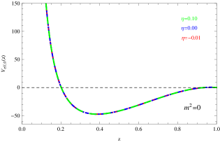
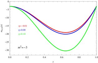
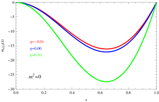
Figure 1: (Color online) The effective potential $V_{eff,0}(z)$ and effective mass $m_{eff,0}(z)$ as a function of the radial coordinate $z$ outside the horizon with the coupling parameter $\eta=-0.01$ (red), 0.00 (blue), and 0.10 (green) for the fixed mass of the scalar field $m^{2}=-3$ (left) and $m^{2}=0$ (right), backreaction parameter $\kappa=0$ and dimensionless quantity $\lambda=10$ in $d=5$ dimensions. It should be noted that the three lines of the effective potential coincide in the top-right panel.

Near the asymptotic boundary $z=0$, we assume that $\psi_{1}$ takes the form Siopsis

$$\psi_{1}(z)\sim\frac{\langle{\cal O}_{i}\rangle}{r^{\Delta_{i}}_{+}}z^{\Delta_{i}}F(z),$$ (29)

where the trial function $F(z)$ obeys the boundary condition $F(0)=1$. Substituting Eq. (29) into Eq. (III), we arrive at

$$\bigg{[}1+\frac{(d-2)\eta z^{2}\xi}{2}\bigg{(}d-3-\frac{z\xi^{\prime}}{\xi}\bigg{)}\bigg{]}F^{\prime\prime}+\bigg{\{}\frac{\xi^{\prime}}{\xi}-\frac{d-4}{z}-Q(z) +$$

$$\frac{2\Delta_{i}}{z}\bigg{[}1+\frac{(d-2)\eta z^{2}\xi}{2}\bigg{(}d-3-\frac{z\xi^{\prime}}{\xi}\bigg{)}\bigg{]}\bigg{\}}F^{\prime}+\bigg{\{}\frac{\Delta_{i}(\Delta_{i}-1)}{z^{2}}\bigg{[}1+\frac{(d-2)\eta z^{2}\xi}{2}\bigg{(}d-3-\frac{z\xi^{\prime}}{\xi}\bigg{)}\bigg{]} +$$

$$\frac{\lambda^{2}(1-z^{d-3})^{2}}{z^{4}\xi^{2}}\bigg{[}1+\frac{(d-2)\eta z^{2}\xi}{2}\bigg{(}d-3-\frac{z\xi^{\prime}}{\xi}\bigg{)}\bigg{]}+\frac{\Delta_{i}}{z}\bigg{[}\frac{\xi^{\prime}}{\xi}-\frac{d-4}{z}-Q(z)\bigg{]}-\frac{m^{2}}{z^{4}\xi}\bigg{\}}F = 0,$$ (30)

with

$$Q(z)=\frac{(d-2)\eta z}{2}\left[(d-3)(d-6)\xi-(3d-13)z\xi^{\prime}+\frac{z^{2}\xi^{\prime 2}}{\xi}+z^{2}\xi^{\prime\prime}\right].$$ (31)

In order to use the Sturm-Lioville method Siopsis , we will adopt an iteration method and express the backreaction parameter $\kappa$ as $\kappa_{n}=n\Delta\kappa$ with $n=0,1,2,\cdot\cdot\cdot$, where $\Delta\kappa=\kappa_{n+1}-\kappa_{n}$ is the step size of our iterative procedure. Setting $\kappa_{-1}=0$ and $\lambda^{2}|_{\kappa_{-1}}=0$, we find that $\kappa^{2}\lambda^{2}=\kappa_{n}^{2}\lambda^{2}=\kappa_{n}^{2}(\lambda^{2}|_{\kappa_{n-1}})+0[(\Delta\kappa)^{4}]$, where $\lambda^{2}|_{\kappa_{n-1}}$ is the value of $\lambda^{2}$ for $\kappa_{n-1}$. Hence we can express the function $\xi(z)$ as

$$\xi(z)\approx\frac{1}{z^{2}}-z^{d-3}-\frac{(d-3)\kappa_{n}^{2}(\lambda^{2}|_{\kappa_{n-1}})}{d-2}z^{d-3}(1-z^{d-3}).$$ (32)

Defining a new function

$$T(z)=z^{4-d+2\Delta_{i}}\xi\bigg{[}1+\frac{(d-2)\eta z^{2}\xi}{2}\bigg{(}d-3-\frac{z\xi^{\prime}}{\xi}\bigg{)}\bigg{]},$$ (33)

we can rewrite Eq. (III) as

$$(TF^{\prime})^{\prime}+z^{4-d+2\Delta_{i}}\xi\bigg{\{}\frac{\Delta_{i}(\Delta_{i}-1)}{z^{2}}\bigg{[}1+\frac{(d-2)\eta z^{2}\xi}{2}\bigg{(}d-3-\frac{z\xi^{\prime}}{\xi}\bigg{)}\bigg{]} +$$

$$\frac{\lambda^{2}(1-z^{d-3})^{2}}{z^{4}\xi^{2}}\bigg{[}1+\frac{(d-2)\eta z^{2}\xi}{2}\bigg{(}d-3-\frac{z\xi^{\prime}}{\xi}\bigg{)}\bigg{]}+\frac{\Delta_{i}}{z}\bigg{(}\frac{\xi^{\prime}}{\xi}-\frac{d-4}{z}-Q\bigg{)}-\frac{m^{2}}{z^{4}\xi}\bigg{\}}F = 0.$$ (34)

According to the Sturm-Liouville eigenvalue problem Gelfand-Fomin , we can deduce the eigenvalue $\lambda$ minimizes the expression

$$\lambda^{2}=\frac{\int^{1}_{0}\left(TF^{\prime 2}-UF^{2}\right)dz}{\int^{1}_{0}VF^{2}dz},$$ (35)

with

$$U(z) = z^{4-d+2\Delta_{i}}\xi\bigg{\{}\frac{\Delta_{i}(\Delta_{i}-1)}{z^{2}}\bigg{[}1+\frac{(d-2)\eta z^{2}\xi}{2}\bigg{(}d-3-\frac{z\xi^{\prime}}{\xi}\bigg{)}\bigg{]}+\frac{\Delta_{i}}{z}\bigg{(}\frac{\xi^{\prime}}{\xi}-\frac{d-4}{z}-Q\bigg{)}-\frac{m^{2}}{z^{4}\xi}\bigg{\}},$$

$$V(z) = \frac{z^{2\Delta_{i}-d}(1-z^{d-3})^{2}}{\xi}\bigg{[}1+\frac{(d-2)\eta z^{2}\xi}{2}\bigg{(}d-3-\frac{z\xi^{\prime}}{\xi}\bigg{)}\bigg{]}.$$ (36)

Using Eq. (35) to calculate the minimum eigenvalue of $\lambda^{2}$ for $i=+$ or $i=-$, we can obtain the critical temperature $T_{c}$ for different coupling parameter $\eta$, strength of the backreaction $\kappa$ and mass of the scalar field $m$ from the following relation

$$T_{c}=\frac{1}{4\pi}\left[(d-1)-\frac{(d-3)^{2}}{d-2}\kappa_{n}^{2}(\lambda^{2}|_{\kappa_{n-1}})\right]\left(\frac{\rho}{\lambda}\right)^{\frac{1}{d-2}}.$$ (37)

For clarity, we focus on the condensate for the operator $\langle{\cal O}_{+}\rangle$, just as mentioned in the previous section. As a matter of fact, another choice for the operator $\langle{\cal O}_{-}\rangle$ will not qualitatively modify our results.

Before going further, we would like to make a comment. In order to get the expression (35), we have used the following boundary condition

$$[T(z)F(z)F^{\prime}(z)]|_{0}^{1}=0.$$ (38)

Obviously, the condition $T(1)F(1)F^{\prime}(1)=0$ can be satisfied easily since we have $T(1)\equiv 0$ from Eq. (33). On the other hand, we observe that the leading order of $z$ in $T(z)$ near $z\rightarrow 0$ is $\beta=2-d+2\Delta_{+}$ in which $\beta\geq 1$ for $m^{2}\geq-(d-1)^{2}[2+(d-1)(d-2)\eta]/8$, which means that the condition $T(0)F(0)F^{\prime}(0)=0$ will be satisfied automatically. Thus, we will just require $F(z)$ to satisfy the Dirichlet boundary condition $F(0)=1$ rather than imposing the Neumann boundary condition $F^{\prime}(0)=0$, just as discussed in HFLi . In the following calculation, we will assume the trial function $F(z)$ to be

$$F(z)=1-az,$$ (39)

where $a$ is a constant. We find that it will give a better estimate of the minimum of (35), which shows that the analytical results are much more closer to the numerical findings.

As an example, we will calculate the case for $\eta=0$, $d=5$ and $m^{2}=-3$ with the chosen values of the backreaction parameter $\kappa$ for the operator $\langle{\cal O}_{+}\rangle$, i.e., $i=+$, and compare with the analytical results in Ref. PanJWCh . Setting the step size $\Delta\kappa=0.05$, for $\kappa_{0}=0$ we arrive at

$$\lambda^{2}=\frac{120(\frac{3}{4}-\frac{9a}{7}-\frac{5a^{2}}{8})}{45+a(184-60\pi)-60\log 2+20a^{2}(-2+\log 8)},$$ (40)

whose minimum is $\lambda^{2}|_{\kappa_{0}}=17.5227$ at $a=0.800597$. From Eq. (37), we can easily obtain the critical temperature $T_{c}=0.197507\rho^{1/3}$, which is much closer to the numerical result $T_{c}=0.197968\rho^{1/3}$ HorowitzPRD78 , compared with the analytical result $T_{c}=0.196209\rho^{1/3}$ from the trial function $F(z)=1-az^{2}$ PanJWCh . For $\kappa_{1}=0.05$, putting $\lambda^{2}|_{\kappa_{0}}$ in Eqs. (32) and (33) we have

$$\lambda^{2}=\frac{1.33528\times 10^{2}(0.744524-1.27459a+0.619159a^{2})}{3.81409-5.03102a+1.77943a^{2}},$$ (41)

whose minimum is $\lambda^{2}|_{\kappa_{1}}=17.4250$ at $a=0.798627$. So the critical temperature reads $T_{c}=0.194805\rho^{1/3}$. Comparing with the analytical result $T_{c}=0.193442\rho^{1/3}$ from Ref. PanJWCh , we find that this value is much closer to the numerical result $T_{c}=0.195293\rho^{1/3}$. For $\kappa_{2}=0.10$, substituting $\lambda^{2}|_{\kappa_{1}}$ into (32) and (33) we get

$$\lambda^{2}=\frac{2.28900\times 10^{6}(0.728219-1.24146a+0.601767a^{2})}{6.63481\times 10^{4}-8.77537a+3.11095\times 10^{4}a^{2}},$$ (42)

whose minimum is $\lambda^{2}|_{\kappa_{2}}=17.1312$ at $a=0.792406$. Therefore the critical temperature is $T_{c}=0.186737\rho^{1/3}$, which is much closer to the numerical finding $T_{c}=0.187414\rho^{1/3}$, compared with the analytical result $T_{c}=0.185189\rho^{1/3}$ in PanJWCh . For other values of $\eta$, $\kappa$, $d$ and $m^{2}$, the similar iterative procedure also can be applied to present the analytical result for the critical temperature.

Table 1: The critical temperature $T_{c}$ obtained by the analytical method (left column) and numerical method (right column) with the chosen values of the coupling parameter $\eta$ and backreaction parameter $\kappa$ for the condensate of the scalar operator in the case of 5-dimensional AdS black hole background. Here we fix the mass of the scalar field by $m^{2}=-3$ and step size by $\Delta\kappa=0.05$.

$\kappa$	0	0.1	0.2
$\eta=-0.01$	$0.201355\rho^{1/3}$   $0.201740\rho^{1/3}$	$0.191578\rho^{1/3}$   $0.192137\rho^{1/3}$	$0.163579\rho^{1/3}$   $0.165238\rho^{1/3}$
$\eta=0$	$0.197507\rho^{1/3}$   $0.197968\rho^{1/3}$	$0.186737\rho^{1/3}$   $0.187414\rho^{1/3}$	$0.156051\rho^{1/3}$   $0.158049\rho^{1/3}$
$\eta=0.01$	$0.194565\rho^{1/3}$   $0.195092\rho^{1/3}$	$0.182953\rho^{1/3}$   $0.183736\rho^{1/3}$	$0.150009\rho^{1/3}$   $0.152312\rho^{1/3}$
$\eta=0.10$	$0.182643\rho^{1/3}$   $0.183528\rho^{1/3}$	$0.166684\rho^{1/3}$   $0.168092\rho^{1/3}$	$0.122372\rho^{1/3}$   $0.126425\rho^{1/3}$
$\eta=0.50$	$0.173569\rho^{1/3}$   $0.174842\rho^{1/3}$	$0.152918\rho^{1/3}$   $0.155093\rho^{1/3}$	$0.096657\rho^{1/3}$   $0.102711\rho^{1/3}$
$\eta=1.00$	$0.171502\rho^{1/3}$   $0.172879\rho^{1/3}$	$0.149553\rho^{1/3}$   $0.151950\rho^{1/3}$	$0.090000\rho^{1/3}$   $0.096586\rho^{1/3}$

Table 2: The critical temperature $T_{c}$ obtained by the analytical method (left column) and numerical method (right column) with the chosen values of the coupling parameter $\eta$ and backreaction parameter $\kappa$ for the condensate of the scalar operator in the case of 4-dimensional AdS black hole background. Here we fix the mass of the scalar field by $m^{2}=-2$ and step size by $\Delta\kappa=0.05$.

$\kappa$	0	0.1	0.2
$\eta=-0.01$	$0.121567\rho^{1/2}$   $0.121763\rho^{1/2}$	$0.118937\rho^{1/2}$   $0.119154\rho^{1/2}$	$0.111255\rho^{1/2}$   $0.111646\rho^{1/2}$
$\eta=0$	$0.118197\rho^{1/2}$   $0.118426\rho^{1/2}$	$0.115330\rho^{1/2}$   $0.115582\rho^{1/2}$	$0.106975\rho^{1/2}$   $0.107435\rho^{1/2}$
$\eta=0.01$	$0.115561\rho^{1/2}$   $0.115822\rho^{1/2}$	$0.112487\rho^{1/2}$   $0.112777\rho^{1/2}$	$0.103553\rho^{1/2}$   $0.104076\rho^{1/2}$
$\eta=0.10$	$0.103856\rho^{1/2}$   $0.104318\rho^{1/2}$	$0.099591\rho^{1/2}$   $0.100111\rho^{1/2}$	$0.087345\rho^{1/2}$   $0.088302\rho^{1/2}$
$\eta=0.50$	$0.092740\rho^{1/2}$   $0.093527\rho^{1/2}$	$0.086689\rho^{1/2}$   $0.087606\rho^{1/2}$	$0.069614\rho^{1/2}$   $0.071322\rho^{1/2}$
$\eta=1.00$	$0.089693\rho^{1/2}$   $0.090597\rho^{1/2}$	$0.082976\rho^{1/2}$   $0.084046\rho^{1/2}$	$0.064117\rho^{1/2}$   $0.066112\rho^{1/2}$

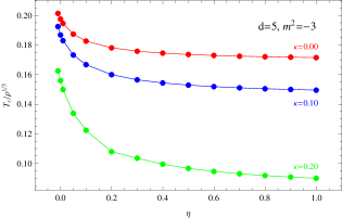
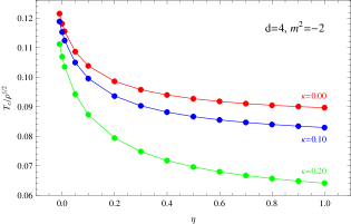
Figure 2: (Color online) The critical temperature $T_{c}$ obtained by the analytical method as a function of the coupling parameter $\eta$ with the fixed mass of the scalar field $m^{2}=-3$ in $d=5$ dimensions (left) and $m^{2}=-2$ in $d=4$ dimensions (right). The three lines from top to bottom correspond to increasing backreaction parameter $\kappa$, i.e., $\kappa=0.00$ (red), 0.10 (blue), and 0.20 (green), respectively.

In order to obtain the effect of the Einstein tensor on the critical temperature for the scalar operator $\langle{\cal O}_{+}\rangle$, we give the critical temperature $T_{c}$ obtained by the analytical Sturm-Liouville method with the fixed masses of the scalar field by $m^{2}=-3$ for the 5-dimensional AdS black hole and $m^{2}=-2$ for the 4-dimensional one in Tables 1 and 2, respectively. In the calculation, we fix the step size by $\Delta\kappa=0.05$. Moreover, to see the dependence of the analytical results on the Einstein tensor more directly, in Fig. 2 we also exhibit the critical temperature $T_{c}$ obtained by the analytical method as a function of the coupling parameter $\eta$ for the fixed backreaction parameters and masses of the scalar field in $d=5$ (left) and $4$ (right) dimensions. For the fixed backreaction parameter, it is clear that with the increase of the coupling parameter $\eta$, the critical temperature $T_{c}$ decreases, which supports the observation obtained in Ref. KuangE2016 and indicates that the Einstein tensor will hinder the condensate of the scalar field. Obviously, the effect of the Einstein tensor on the condensate of the scalar field is consistent with the behavior of the effective potential shown in Fig. 1. On the other hand, imposing the Dirichlet boundary condition of the trial function $F(z)$ without the Neumann boundary conditions, we observe that the improved Sturm-Liouville method can indeed give a better estimate of the critical temperature, compared with the analytical result from the trial function $F(z)=1-az^{2}$ in Ref. PanJWCh .

Table 3: The critical temperature $T_{c}$ obtained by the analytical method (left column) and numerical method (right column) with the chosen values of the coupling parameter $\eta$ and backreaction parameter $\kappa$ for the condensate of the scalar operator in the case of 5-dimensional AdS black hole background. Here we fix the mass of the scalar field by $m^{2}=0$ and step size by $\Delta\kappa=0.05$.

$\kappa$	0	0.1	0.2
$\eta=-0.01$	$0.168998\rho^{1/3}$   $0.170509\rho^{1/3}$	$0.145743\rho^{1/3}$   $0.148561\rho^{1/3}$	$0.085189\rho^{1/3}$   $0.093255\rho^{1/3}$
$\eta=0$	$0.168998\rho^{1/3}$   $0.170509\rho^{1/3}$	$0.145719\rho^{1/3}$   $0.148530\rho^{1/3}$	$0.084974\rho^{1/3}$   $0.093006\rho^{1/3}$
$\eta=0.01$	$0.168998\rho^{1/3}$   $0.170509\rho^{1/3}$	$0.145697\rho^{1/3}$   $0.148502\rho^{1/3}$	$0.084782\rho^{1/3}$   $0.092783\rho^{1/3}$
$\eta=0.10$	$0.168998\rho^{1/3}$   $0.170509\rho^{1/3}$	$0.145576\rho^{1/3}$   $0.148345\rho^{1/3}$	$0.083683\rho^{1/3}$   $0.091482\rho^{1/3}$
$\eta=0.50$	$0.168998\rho^{1/3}$   $0.170509\rho^{1/3}$	$0.145432\rho^{1/3}$   $0.148158\rho^{1/3}$	$0.082343\rho^{1/3}$   $0.089839\rho^{1/3}$
$\eta=1.00$	$0.168998\rho^{1/3}$   $0.170509\rho^{1/3}$	$0.145391\rho^{1/3}$   $0.148104\rho^{1/3}$	$0.081952\rho^{1/3}$   $0.089346\rho^{1/3}$

Table 4: The critical temperature $T_{c}$ obtained by the analytical method (left column) and numerical method (right column) with the chosen values of the coupling parameter $\eta$ and backreaction parameter $\kappa$ for the condensate of the scalar operator in the case of 4-dimensional AdS black hole background. Here we fix the mass of the scalar field by $m^{2}=0$ and step size by $\Delta\kappa=0.05$.

$\kappa$	0	0.1	0.2
$\eta=-0.01$	$0.085581\rho^{1/2}$   $0.086667\rho^{1/2}$	$0.078022\rho^{1/2}$   $0.079368\rho^{1/2}$	$0.057473\rho^{1/2}$   $0.060125\rho^{1/2}$
$\eta=0$	$0.085581\rho^{1/2}$   $0.086667\rho^{1/2}$	$0.078015\rho^{1/2}$   $0.079360\rho^{1/2}$	$0.057433\rho^{1/2}$   $0.060080\rho^{1/2}$
$\eta=0.01$	$0.085581\rho^{1/2}$   $0.086667\rho^{1/2}$	$0.078009\rho^{1/2}$   $0.079353\rho^{1/2}$	$0.057394\rho^{1/2}$   $0.060037\rho^{1/2}$
$\eta=0.10$	$0.085581\rho^{1/2}$   $0.086667\rho^{1/2}$	$0.077963\rho^{1/2}$   $0.079303\rho^{1/2}$	$0.057125\rho^{1/2}$   $0.059734\rho^{1/2}$
$\eta=0.50$	$0.085581\rho^{1/2}$   $0.086667\rho^{1/2}$	$0.077886\rho^{1/2}$   $0.079211\rho^{1/2}$	$0.056619\rho^{1/2}$   $0.059156\rho^{1/2}$
$\eta=1.00$	$0.085581\rho^{1/2}$   $0.086667\rho^{1/2}$	$0.077839\rho^{1/2}$   $0.079173\rho^{1/2}$	$0.056408\rho^{1/2}$   $0.058911\rho^{1/2}$

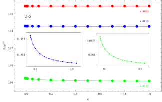
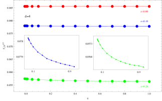
Figure 3: (Color online) The critical temperature $T_{c}$ obtained by the analytical method as a function of the coupling parameter $\eta$ with the fixed mass of the scalar field $m^{2}=0$ in $d=5$ (left) and $4$ (right) dimensions. The three lines from top to bottom correspond to increasing backreaction parameter $\kappa$, i.e., $\kappa=0.00$ (red), 0.10 (blue), and 0.20 (green), respectively.

Considering the fact that the effect of the Einstein tensor is intertwined with that of the mass of the scalar field in the expression (11), we will set $m^{2}=0$ to get the pure effect of the Einstein tensor on the critical temperature. In Tables 3, 4 and Fig. 3, we provide the critical temperature $T_{c}$ obtained by the analytical Sturm-Liouville method with the fixed mass of the scalar field by $m^{2}=0$ and step size by $\Delta\kappa=0.05$ for the 5- and 4-dimensional AdS black hole backgrounds respectively. For the fixed nonzero parameter $\kappa$, the conclusion still holds, i.e., the Einstein tensor hinders the condensate of the scalar field. However, for the probe limit $\kappa=0$, from the leftmost columns in Tables 3, 4 and the red lines in Fig. 3 we find that $T_{c}$ is independent of the coupling parameter $\eta$, which implies that the Einstein tensor will not affect the condensate of the scalar field for the case of $m^{2}=0$. Again, in this case the effect of the Einstein tensor on the condensate of the scalar field agrees well with the behavior of the effective potential shown in Fig. 1. Thus, the probe approximation loses some important information and we have to count on the backreaction to explore the real impact of the Einstein tensor on the holographic superconductors in this case. Moreover, in the case of $m^{2}=0$, we observe that the critical temperature $T_{c}$ increases as the spacetime dimension $d$ increases for the fixed coupling parameter $\eta$ and backreaction parameter $\kappa$, which supports the findings in Ref. Pan-WangGB2010 and means that the increase of the dimensionality of the AdS space makes it easier for the scalar hair to be formed.

On the other hand, from Tables 1-4 and Figs. 2-3, we point out that the critical temperature $T_{c}$ decreases as the backreaction parameter $\kappa$ increases for the fixed coupling parameter $\eta$, scalar field mass $m^{2}$ and spacetime dimension $d$, which shows that the stronger backreaction can make the scalar hair more difficult to be developed. This can be used to back up the findings in Refs. PanJWCh ; BarclayGregory ; Barclay2011 ; GregoryRev ; KannoCQG ; CSJHEP2015 .

IV Critical behavior from marginally stable modes

We now use the shooting method HartnollRev ; HerzogRev ; HorowitzRev ; CaiRev to study the marginally stable modes of the scalar perturbation coupled to the electric field and Einstein tensor, which can reveal the critical behavior of the holographic superconductors with backreactions from the coupling of a scalar field to the Einstein tensor near the phase transition point numerically. We will also compare this numerical result with the analytical one in order to test the effectiveness and accuracy of the Sturm-Liouville method.

Considering the scalar perturbation in the Reissner-Nordström AdS black hole background (12) coupled to a Maxwell field and Einstein tensor, from the action (1) we can get the Euler-Lagrange equation of motion for the perturbation field

$$\frac{1}{\sqrt{-g}}(\partial_{\mu}-iA_{\mu})\left[\sqrt{-g}(g^{\mu\nu}+\eta G^{\mu\nu})(\partial_{\nu}-iA_{\nu})\right]\tilde{\psi}-m^{2}\tilde{\psi}=0,$$ (43)

with the nonzero components of the Einstein tensor

$$G^{tt}=-\frac{d-2}{2r^{2}}\left[(d-3)+\frac{rf^{\prime}}{f}\right],~{}~{}G^{rr}=\frac{(d-2)f^{2}}{2r^{2}}\left[(d-3)+\frac{rf^{\prime}}{f}\right],$$

$$G^{xx}=G^{yy}=\cdot\cdot\cdot=\frac{(d-3)(d-4)f+r[2(d-3)f^{\prime}+rf^{\prime\prime}]}{2r^{4}},$$ (44)

where $f$ is given by (12). Assuming $\tilde{\psi}=e^{-i\omega t}R(r)Y(x^{i})$ and making the separation of the variables, we obtain

$$\left\{1+\frac{(d-2)\eta}{2r}\bigg{[}f^{\prime}+\frac{(d-3)f}{r}\bigg{]}\right\}R^{\prime\prime}+\bigg{\{}\left(\frac{d-2}{r}+\frac{f^{\prime}}{f}\right)+\frac{(d-2)\eta}{2r} \times$$

$$\bigg{[}f^{\prime\prime}+\frac{3(d-3)f^{\prime}}{r}+\frac{f^{\prime 2}}{f}+\frac{(d-3)(d-4)f}{r^{2}}\bigg{]}\bigg{\}}R^{\prime}+\frac{(\phi+\omega)^{2}}{f^{2}}\left\{1+\frac{(d-2)\eta}{2r}\bigg{[}f^{\prime}+\frac{(d-3)f}{r}\bigg{]}\right\}R -$$

$$\frac{A_{n}^{2}}{r^{2}f}\left\{1+\frac{\eta}{2}\bigg{[}f^{\prime\prime}+\frac{2(d-3)f^{\prime}}{r}+\frac{(d-3)(d-4)f}{r^{2}}\bigg{]}\right\}R-\frac{m^{2}}{f}R = 0,$$ (45)

where $\phi$ has been introduced in (12) and $A_{n}\in\mathbb{Z}$ is the eigenvalue of the following equation

$$\Sigma_{i}\left[\frac{\partial^{2}Y(x^{i})}{\partial x^{i2}}\right]+A_{n}^{2}\Sigma_{i}Y(x^{i})=0,$$ (46)

with $x^{i}=x,y,\cdots$. It is expected that the lowest mode $A_{n}=0$ will be the first to condense and result in the most stable solution after condensing, which means that there are no momenta in the $(x,y,...)$-directions marginally stable modes . Then, changing the variable from $r$ to $z=r_{+}/r$ for convenience, we have the equation of motion

$$\left\{1+\frac{(d-2)\eta z^{2}f}{2r_{+}^{2}}\bigg{[}(d-3)-\frac{zf^{\prime}}{f}\bigg{]}\right\}R^{\prime\prime}-\bigg{\{}\left(\frac{d-4}{z}-\frac{f^{\prime}}{f}\right)+\frac{(d-2)\eta z}{2r_{+}^{2}}\bigg{[}z^{2}f^{\prime\prime}-(3d-13)zf^{\prime} +$$

$$\frac{z^{2}f^{\prime 2}}{f}+(d-3)(d-6)f\bigg{]}\bigg{\}}R^{\prime}+\frac{r_{+}^{2}(\phi+\omega)^{2}}{z^{4}f^{2}}\bigg{\{}1+\frac{(d-2)\eta z^{2}f}{2r_{+}^{2}}\bigg{[}(d-3)-\frac{zf^{\prime}}{f}\bigg{]}\bigg{\}}R-\frac{m^{2}r_{+}^{2}}{z^{4}f}R = 0,$$ (47)

where the prime now denotes the derivative with respect to $z$.

It is well known that the marginally stable modes correspond to $\omega=0$ which indicates that the phase transition or the critical phenomena may occur GubserPRD78 . Thus, we will solve the equation of motion (IV) numerically by doing integration from the horizon out to the infinity in the case of $\omega=0$ with the boundary conditions of $R(z)$ at the event horizon

$$R(z)=R(1)-R^{\prime}(1)(1-z)+\frac{1}{2}R^{\prime\prime}(1)(1-z)^{2}+\cdots\,,$$ (48)

and at the asymptotic AdS boundary

$$R(z)=\frac{R_{-}}{r^{\Delta_{-}}_{+}}z^{\Delta_{-}}+\frac{R_{+}}{r_{+}^{\Delta_{+}}}z^{\Delta_{+}}.$$ (49)

Since we concentrate on the condensate for the operator $\langle{\cal O}_{+}\rangle$ in this work, we impose boundary condition $R_{-}=0$. In the following calculations, we will scan the parameter space of holographic superconductors and find the certain values of $\lambda=\rho/r^{d-2}_{+c}$ which satisfy the boundary condition for the given $\eta$, $\kappa$, $m^{2}$ and $d$. Note that the quantity of $R(1)$ is very close to zero near the critical point of the phase transition, we set the initial condition $R(1)=0.001$ without loss of generality.

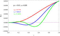
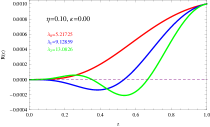
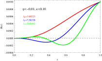
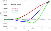
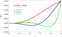
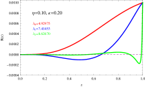
Figure 4: (Color online.) The marginally stable curves of scalar fields corresponding to various critical values $\lambda_{n}$ with $m^{2}=-3$ for different coupling parameters $\eta$ and backreaction parameters $\kappa$ in the case of 5-dimensional AdS black hole background. The first three lowest-lying critical values $\lambda_{n}$ for different curves are $\lambda_{0}<\lambda_{1}<\lambda_{2}$ in the sequence.

In Fig. 4, we plot the marginally stable curves of scalar fields $R(z)$ corresponding to the critical values $\lambda_{n}$ with $m^{2}=-3$ for different coupling parameters $\eta$ and backreaction parameters $\kappa$ in the case of 5-dimensional AdS black hole background by solving Eq. (IV) numerically. In each panel, three curves correspond to the first three lowest-lying critical values $\lambda_{n}$ which are $\lambda_{0}<\lambda_{1}<\lambda_{2}$ in the sequence, where the index $n$ denotes the “overtone number” marginally stable modes . The red line has no intersecting points with the $R(z)=0$ axis at nonvanishing $z$ and is dual to the minimal value of $\lambda_{n}$ (a mode of node $n=0$), which will be the first to condense. The blue line (a mode of node $n=1$) has one intersecting point with $R(z)=0$ axis while the green line (a mode of node $n=2$) has two, which do not matter to the phase transition because the blue and green lines are expected to be unstable with radial oscillations in $z$-direction of $R(z)$ costing energy GubserPufu . At the critical point, inserting $\lambda_{0}$ into the Hawking temperature of the $d$-dimensional Reissner-Nordström black hole (12), i.e.,

$$T_{H}=\frac{r_{+}}{4\pi}\left[(d-1)-\frac{(d-3)^{2}\kappa^{2}}{d-2}\left(\frac{\rho}{r^{d-2}_{+}}\right)^{2}\right],$$ (50)

we can easily obtain the critical temperature $T_{c}$. For example, for the case of $\eta=0.00,~{}\kappa=0.10$ with $m^{2}=-3$ and $d=5$, from Fig. 4 we have $\lambda_{0}=4.11554$, which leads to $T_{c}=0.187414\rho^{1/3}$. Similarly, we can get the critical temperatures for different values of $\eta$, $\kappa$, $d$ and $m^{2}$.

In Tables 1-4, we present the critical temperatures obtained numerically by using the shooting method for the 5-dimensional and 4-dimensional black hole backgrounds, respectively. Compared with the analytical results in each table, the agreement of the numerical calculation (right column) and analytical result derived from the Sturm-Liouville method (left column) is impressive, which implies that the Sturm-Liouville method is still powerful to study the holographic superconductors from the coupling of a scalar field to the Einstein tensor even if we consider the backreactions. Obviously, the “marginally stable modes” method is a very effective way to study the critical behavior of the phase transition in the holographic superconductor models. In addition to giving us the numerical results of the critical temperature, the marginally stable modes can reveal the instabilities of the background which means that the AdS black hole will become unstable to develop charged scalar hairs in the AdS black hole background.

V Conclusions

We have investigated the properties of the backreacting holographic superconductors from the coupling of a scalar field to the Einstein tensor in the background of a $d$-dimensional AdS black hole, which provides a more explicit and complete understanding of the effect of the Einstein tensor on the holographic superconductors. Imposing the Dirichlet boundary condition of the trial function $F(z)$ without the Neumann boundary conditions, we improved the analytical Sturm-Liouville method with an iterative procedure to calculate the critical temperatures for the scalar operator $\langle{\cal O}_{+}\rangle$ and found that the analytical findings obtained in this way are in very good agreement with the numerical results from the “marginally stable modes” method, which implies that the Sturm-Liouville method is still powerful to study the holographic superconductors from the coupling of a scalar field to the Einstein tensor even if we consider the backreactions. It is shown that, when the backreaction parameter is nonzero, the critical temperature decreases with the increase of the coupling parameter of the Einstein tensor, which can be used to back up the observation obtained in Ref. KuangE2016 that the Einstein tensor will hinder the condensate of the scalar field. However, when the backreaction parameter and scalar mass are zero, the critical temperature is independent of the Einstein tensor, which implies that the probe approximation still loses some important information and we have to count on the backreaction to explore the real and pure impact of the Einstein tensor on the holographic superconductors in this case. In addition, we observed that the critical temperature increases as the spacetime dimension increases for the fixed scalar mass, coupling parameter and backreaction parameter, which means that the scalar hair can be formed easier in the higher-dimensional background. Moreover, we interestingly noted that the Einstein tensor, backreaction and spacetime dimension cannot modify the critical phenomena, i.e., this holographic superconductor phase transition belongs to the second order and the critical exponent of the system always takes the mean-field value.

References

• (1) M. Tinkham, Introduction to Superconductivity, 2nd ed.(McGrawHill, New York, 1996).
• (2) J. Bardeen, L.N. Cooper, and J.R. Schrieffer, Phys. Rev. 108, 1175 (1957).
• (3) J. Maldacena, Adv. Theor. Math. Phys. 2, 231 (1998) [Int. J. Theor. Phys. 38, 1113 (1999)].
• (4) S.S. Gubser, I.R. Klebanov, and A.M. Polyakov, Phys. Lett. B 428, 105 (1998).
• (5) E. Witten, Adv. Theor. Math. Phys. 2, 253 (1998).
• (6) S.S. Gubser, Phys. Rev. D 78, 065034 (2008).
• (7) S.A. Hartnoll, C.P. Herzog, and G.T. Horowitz, Phys. Rev. Lett. 101, 031601 (2008).
• (8) S.A. Hartnoll, C.P. Herzog, and G.T. Horowitz, J. High Energy Phys. 12, 015 (2008).
• (9) Q.Y. Pan, J.L. Jing, B. Wang, and S.B. Chen, J. High Energy Phys. 06, 087 (2012).
• (10) L. Barclay, R. Gregory, S. Kanno, and P. Sutcliffe, J. High Energy Phys. 12, 029 (2010); arXiv:1009.1991 [hep-th].
• (11) L. Barclay, J. High Energy Phys. 10, 044 (2011).
• (12) R. Gregory, J. Phys. Conf. Ser. 283, 012016 (2011); arXiv:1012.1558 [hep-th].
• (13) S. Kanno, Class. Quant. Grav. 28, 127001 (2011); arXiv:1103.5022 [hep-th].
• (14) X.H. Ge and H.Q. Leng, Prog. Theor. Phys. 128, 1211 (2012); arXiv:1105.4333 [hep-th].
• (15) C.P. Herzog, Phys. Rev. D 81, 126009 (2010); arXiv:1003.3278 [hep-th].
• (16) S.S. Gubser and A. Nellore, J. High Energy Phys. 04, 008 (2009).
• (17) G.T. Horowitz and B. Way, J. High Energy Phys. 11, 011 (2010); arXiv:1007.3714 [hep-th].
• (18) F. Aprile and J.G. Russo, Phys. Rev. D 81, 026009 (2010).
• (19) Y. Brihaye and B. Hartmann, Phys. Rev. D 81, 126008 (2010).
• (20) Y. Liu and Y.W. Sun, J. High Energy Phys. 07, 099 (2010).
• (21) M. Siani, J. High Energy Phys. 12, 035 (2010); arXiv:1010.0700 [hep-th].
• (22) Q.Y. Pan and B. Wang, arXiv:1101.0222 [hep-th].
• (23) Y.Q. Liu, Q.Y. Pan, and B. Wang, Phys. Lett. B 702, 94 (2011).
• (24) Y.Q. Liu, Y. Peng, and B. Wang, arXiv:1202.3586 [hep-th].
• (25) S. Gangopadhyay, Phys. Lett. B 724, 176 (2013); arXiv:1302.1288 [hep-th].
• (26) Y.Q. Liu, Y.G. Gong, and B. Wang, J. High Energy Phys. 02, 116 (2016); arXiv:1505.03603 [hep-ph].
• (27) W.P. Yao and J.L. Jing, J. High Energy Phys. 05, 101 (2013); J. High Energy Phys. 05, 058 (2014); Nucl. Phys. B 889, 109 (2014); Phys. Lett. B 759, 533 (2016).
• (28) R. Emparan and K. Tanabe, J. High Energy Phys. 01, 145 (2014); arXiv:1312.1108 [hep-th].
• (29) A. Dey, S. Mahapatra, and T. Sarkar, J. High Energy Phys. 06, 147 (2014); arXiv:1404.2190 [hep-th].
• (30) L. Nakonieczny and M. Rogatko, Phys. Rev. D 90, 106004 (2014); arXiv:1411.0798 [hep-th].
• (31) D. Momeni, H. Gholizade, M. Raza, and R. Myrzakulov, Phys. Lett. B 747, 417 (2015); arXiv:1503.02896 [hep-th].
• (32) D. Ghorai and S. Gangopadhyay, Eur. Phys. J. C 76, 146 (2016).
• (33) J.L. Jing, L. Jiang, and Q.Y. Pan, Class. Quant. Grav. 33, 025001 (2016).
• (34) A. Sheykhi and F. Shaker, Phys. Lett. B 754, 281 (2016).
• (35) Y. Peng, Q.Y. Pan, and Y.Q. Liu, Nucl. Phys. B 915, 69 (2017).
• (36) A. Sheykhi and F. Shaker, Int. J. Mod. Phys. D 26, 1750050 (2017).
• (37) Z. Sherkatghanad, B. Mirza, and F.L. Dezaki, Int. J. Mod. Phys. D 26, 1750175 (2017).
• (38) W.P. Yao, C.H. Yang, and J.L. Jing, Eur. Phys. J. C 78, 353 (2018); arXiv:1805.02328 [gr-qc].
• (39) B.B. Ghotbabadi, M.K. Zangeneh, and A. Sheykhi, Eur. Phys. J. C 78, 381 (2018).
• (40) D. Ghorai and S. Gangopadhyay, Nucl. Phys. B 933, 1 (2018).
• (41) M. Mohammadi, A. Sheykhi, and M.K. Zangeneh, arXiv:1805.07377 [hep-th].
• (42) R.G. Cai, Z.Y. Nie, and H.Q. Zhang, Phys. Rev. D 83, 066013 (2011); arXiv:1012.5559 [hep-th].
• (43) R.E. Arias and I.S. Landea, J. High Energy Phys. 01, 157 (2013); arXiv:1210.6823 [hep-th].
• (44) R.G. Cai, L. Li, and L.F. Li, J. High Energy Phys. 01, 032 (2014); arXiv:1309.4877 [hep-th].
• (45) R.G. Cai, L. Li, L.F. Li, and R.Q. Yang, J. High Energy Phys. 04, 016 (2014); arXiv:1401.3974 [gr-qc].
• (46) P. Chaturvedi and G. Sengupta, J. High Energy Phys. 04, 001 (2015).
• (47) Z.Y. Nie, R.G. Cai, X. Gao, L. Li, and H. Zeng, Eur. Phys. J. C 75, 559 (2015); arXiv:1501.00004 [hep-th].
• (48) Y.Q. Wang and S. Liu, J. High Energy Phys. 11, 127 (2016).
• (49) Z.Y. Nie, Q.Y. Pan, H.B. Zeng, and H. Zeng, Eur. Phys. J. C 77, 69 (2017); arXiv:1611.07278 [hep-th].
• (50) X.H. Ge, S.F. Tu, and B. Wang, J. High Energy Phys. 09, 088 (2012); arXiv:1209.4272 [hep-th].
• (51) S.A. Hartnoll, Class. Quant. Grav. 26, 224002 (2009).
• (52) C.P. Herzog, J. Phys. A 42, 343001 (2009).
• (53) G.T. Horowitz, Lect. Notes Phys. 828 313, (2011); arXiv:1002.1722 [hep-th].
• (54) R.G. Cai, L. Li, L.F. Li, and R.Q. Yang, Sci. China Phys. Mech. Astron. 58, 060401 (2015); arXiv:1502.00437 [hep-th].
• (55) A.V. Balatsky, I. Vekhter, and J.X. Zhu, Rev. Mod. Phys. 78, 373 (2006).
• (56) T. Ishii and S.J. Sin, J. High Energy Phys. 04, 128 (2013); arXiv:1211.1798 [hep-th].
• (57) H.B. Zeng and H.Q. Zhang, Nucl. Phys. B 897, 276 (2015); arXiv:1411.3955 [hep-th].
• (58) L.Q. Fang, X.M. Kuang, B. Wang, and J.P. Wu, J. High Energy Phys. 11, 134 (2015).
• (59) X.M. Kuang and E. Papantonopoulos, J. High Energy Phys. 08, 161 (2016); arXiv:1607.04928 [hep-th].
• (60) G. Siopsis and J. Therrien, J. High Energy Phys. 05, 013 (2010).
• (61) G. Siopsis, J. Therrien, and S. Musiri, Class. Quant. Grav. 29, 085007 (2012); arXiv:1011.2938 [hep-th].
• (62) R.G. Cai, X. He, H.F. Li, and H.Q. Zhang, Phys. Rev. D 84, 046001 (2011).
• (63) P. Breitenloher and D. Z. Freedman, Ann. Phys. 144, 249 (1982).
• (64) T. Kolyvaris, G. Koutsoumbas, E. Papantonopoulos, and G. Siopsis, Class. Quant. Grav. 29, 205011 (2012); arXiv:1111.0263 [gr-qc].
• (65) T. Kolyvaris, G. Koutsoumbas, E. Papantonopoulos, and G. Siopsis, J. High Energy Phys. 11, 133 (2013); arXiv:1308.5280 [hep-th].
• (66) I.M. Gelfand and S.V. Fomin, Calculaus of Variations, Revised English Edition, Translated and Edited by R.A. Silverman, Prentice-Hall, Inc. Englewood Cliff, New Jersey (1963).
• (67) H.F. Li, J. High Energy Phys. 07, 135 (2013); arXiv:1306.3071 [hep-th].
• (68) G.T. Horowitz and M.M. Roberts, Phys. Rev. D 78, 126008 (2008).
• (69) Q.Y. Pan, B. Wang, E. Papantonopoulos, J. Oliveria, and A.B. Pavan, Phys. Rev. D 81, 106007 (2010).
• (70) S.S. Gubser and S.S. Pufu, J. High Energy Phys. 11, 033 (2008).