1 Introduction

Mixtures of particles in the quantum regime have been a topic of research in various fields of physics, starting from experiments on liquid helium mixtures [1, 2]. With the development of ultracold atom experiments, it has been possible to realise mixtures of atoms at low temperature and study their properties with full control over their parameters such as density and interactions. Originally, the experiments focused on the more stable mixtures of bosonic atoms with repulsive interactions [3, 4, 5, 6]. These experiments exhibited the phenomenon of phase separation for large enough interspecies repulsion, as anticipated by theoretical works based on the mean-field approximation [7, 8, 9, 10, 11, 12]. More recently, there has been an interest in mixtures of bosonic atoms with attractive interactions [13, 14, 15], originally thought to be unstable, after it was discovered that they can form self-bound liquid droplets [16]. Even the properties of a single or a few particles mixed with another kind of particles constitute a challenging problem for theory. Such impurities immersed in a medium become quasi-particles known as polarons, and have been the subject of recent experimental investigations both in fermionic [17, 18, 19, 20, 21, 22, 23] and bosonic [24, 25, 26, 27, 28, 29, 30] ultracold atomic media, as well as many related theoretical works [31, 32, 33, 34, 35, 36, 37, 38, 39, 40, 41, 42, 43, 44, 45, 46, 47, 48, 49, 50, 51, 52, 53, 54, 55, 56, 57, 58, 59, 60, 61, 62, 63, 64, 65, 66, 67, 68, 69, 70, 71, 72, 73]. One compelling aspect of these polarons is their effective interactions mediated by the medium [74, 75].

So far, theoretical works have focused on the pairwise interactions induced by the medium. In this work, it is shown that the medium may also induce three-body interactions, which can have a crucial effect on the macroscopic properties of the impurities. In the case of bosonic impurities immersed in a Bose-Einstein condensate, a bubble of polarons can be formed and stabilised by these three-body interactions. This paper first gives an exact calculation of the induced two-body and three-body interactions between impurities induced by the surrounding condensate, in the specific limit of infinitely heavy impurities and perturbative interactions. In a second step, a simple mean-field theory is used to characterise the resulting state formed by the impurities. Finally, a possible implementation with ultracold atoms is discussed.

2 Mediated interactions

Let us consider a system of $N_{I}$ particles of mass $M$, referred to as impurities, immersed in a homogeneous gas of $N_{B}$ bosonic particles of mass $m$, referred to as bosons. This system is described in the second-quantisation formalism by the following Hamiltonian,

$$H = \sum_{\bm{k}}\epsilon_{k}b_{\bm{k}}^{\dagger}b_{\bm{k}}+\frac{1}{2V}\sum_{\bm{k},\bm{k}^{\prime},\bm{p}}U_{B}(\bm{p})b_{\bm{k^{\prime}-p}}^{\dagger}b_{\bm{k+p}}^{\dagger}b_{\bm{k}}b_{\bm{k}^{\prime}}$$ (1)

$$+\sum_{\bm{k}}\varepsilon_{k}c_{\bm{k}}^{\dagger}c_{\bm{k}}+\frac{1}{2V}\sum_{\bm{k},\bm{k}^{\prime},\bm{p}}U_{I}(\bm{p})c_{\bm{k^{\prime}-p}}^{\dagger}c_{\bm{k+p}}^{\dagger}c_{\bm{k}}c_{\bm{k}^{\prime}}$$

$$+\frac{1}{V}\sum_{\bm{k},\bm{k}^{\prime},\bm{p}}U(\bm{p})b_{\bm{k^{\prime}-p}}^{\dagger}c_{\bm{k}+\bm{p}}^{\dagger}c_{\bm{k}}b_{\bm{k}^{\prime}}$$

where $V$ is the system’s volume, $\epsilon_{k}=\frac{\hbar^{2}k^{2}}{2m}$ and $b_{\bm{k}}$ are the kinetic energy and annihilation operator for a boson with momentum $\bm{k}$, and $\varepsilon_{k}=\frac{\hbar^{2}k^{2}}{2M}$ and $c_{\bm{k}}$ are the kinetic energy and annihilation operator for an impurity with momentum $\bm{k}$. The potential $U_{B}$ and $U_{I}$ describe the interaction between two bosons, and between two impurities, respectively, while the potential $U$ describes the interactions between a boson and an impurity. The potential $U_{B}$ is assumed to be repulsive to guarantee the stability of the medium of condensed bosons. Moreover, all potentials $U_{B}$, $U_{I}$, and $U$ are assumed to be in the perturbative regime satisfying the Born approximation [76], i.e. their respective scattering lengths $a_{B}$, $a_{I}$, and $a$ can be expanded in a convergent perturbative series of the form $a=a_{1}+a_{2}+a_{3}+\dots$that is dominated by the first-order term $a_{1}=\frac{2\mu}{4\pi\hbar^{2}}U(\bm{0})$, where $\mu$ is the reduced mass of the considered particles. For interactions $U(\bm{k})$ that become negligible for $k\gtrsim\Lambda$, where $\Lambda^{-1}$ corresponds to the range of the interaction (for instance, the nanometre range for neutral atoms), then $a_{2}\approx-a_{1}^{2}\frac{2}{\pi}\Lambda$ and the Born approximation requires that the scattering length $a_{1}$ be much smaller than the range $\Lambda^{-1}$.

In this regime, the bosons can be treated with the Bogoliubov approach [77, 12], which consists in applying the following substitution,

$$b_{\bm{0}} \equiv\sqrt{N_{0}}$$ (2)

$$b_{\bm{k}} \equiv u_{k}\beta_{\bm{k}}-v_{k}\beta_{-\bm{k}}^{\dagger}\qquad\text{for }\bm{k}\neq\bm{0}$$ (3)

where $N_{0}$ represents the macroscopic number of bosons occupying the condensate mode $\bm{k}=\bm{0}$, and $\beta_{\bm{k}}$ is the annihilation operator for bosonic quasi-particles (Bogoliubov quasi-particles), corresponding to elementary excitations of the bosonic system. The coefficients $u_{k}$ and $v_{k}$ are chosen to diagonalise the quadratic form in $\beta$ and $\beta^{\dagger}$ appearing in the first line of Eq. (1) when the substitution is applied. The Hamiltonian then reads $H=H^{(\text{F})}+H^{(\text{NF})}$ with

$$H^{(\text{F})}= E_{0}+{\displaystyle\sum_{\bm{k}\neq\bm{0}}E_{k}\beta_{\bm{k}}^{\dagger}\beta_{\bm{k}}}+H^{\prime}$$

$$+\sum_{\bm{k}}(\varepsilon_{k}+n_{B}U(\bm{0}))c_{\bm{k}}^{\dagger}c_{\bm{k}}+\sum_{\bm{k}}C_{\bm{k}}(\beta_{\bm{k}}^{\dagger}+\beta_{-\bm{k}})n_{\bm{k}}$$

$$+\frac{1}{2V}\sum_{\bm{k},\bm{k}^{\prime},\bm{p}}U_{I}(\bm{p})c_{\bm{k^{\prime}-p}}^{\dagger}c_{\bm{k+p}}^{\dagger}c_{\bm{k}}c_{\bm{k}^{\prime}},$$ (4)

$$H^{(\text{NF})} ={\displaystyle\frac{1}{V}\sum_{\bm{p}\neq\bm{0}}\sum_{\bm{k}\neq\bm{0},-\bm{p}}\bigg{(}A_{\bm{k},\bm{p}}\beta_{\bm{k}+\bm{p}}^{\dagger}\beta_{\bm{k}}}$$

$$-B_{\bm{k},\bm{p}}\left(\beta_{-\bm{k}-\bm{p}}\beta_{\bm{k}}+\beta_{\bm{k}+\bm{p}}^{\dagger}\beta_{-\bm{k}}^{\dagger}\right)\bigg{)}n_{\bm{p}},$$ (5)

where $E_{0}\approx\frac{1}{2}U_{B}(\bm{0})Vn_{0}^{2}$ and $E_{k}=\sqrt{\epsilon_{k}(\epsilon_{k}+2n_{0}U_{B}(0))}$ are the Bogoliubov ground-state and excitation energies, and $n_{0}=N_{0}/V$ and $n_{B}=N_{B}/V$ are the condensate and total densities of bosons. In the perturbative limit of small $U_{B}$, the term $H^{\prime}$ , which contains orders higher than quadratic in $\beta$ and $\beta^{\dagger}$, may be neglected. Likewise, the condensate is almost pure, and $n_{0}$ may be approximated by $n_{B}$. In Eqs. (4-5), the notation $n_{\bm{k}}\equiv\sum_{\bm{p}}c_{\bm{p}-\bm{k}}^{\dagger}c_{\bm{p}}=n_{-\bm{k}}^{\dagger}$ has been used, and the coefficients $A_{\bm{k},\bm{p}}$, $B_{\bm{k},\bm{p}}$, and $C_{\bm{k}}$ are given by the following expressions,

$$A_{\bm{k},\bm{p}} \equiv U(\bm{p})\left(u_{|\bm{k}+\bm{p}|}u_{k}+v_{|\bm{k}+\bm{p}|}v_{k}\right)$$ (6)

$$B_{\bm{k},\bm{p}} \equiv U(\bm{p})u_{|\bm{k}+\bm{p}|}v_{k}$$ (7)

$$C_{\bm{k}}\equiv \frac{1}{V}\sqrt{N_{0}}U(\bm{k})(u_{k}-v_{k})$$ (8)

where the Bogoliubov amplitudes $u_{k}$ and $v_{k}$ are given by $u_{k}^{2}=\frac{1}{2}\left(\frac{\epsilon_{k}+n_{0}U_{B}(\bm{0})}{E_{k}}+1\right)$ and $v_{k}^{2}=\frac{1}{2}\left(\frac{\epsilon_{k}+n_{0}U_{B}(\bm{0})}{E_{k}}-1\right)$.

The Hamiltonian $H^{(\text{F})}$ of Eq. (4) corresponds to the Fröhlich polaron model [78, 79], in which impurities can move in the bosonic medium and either create or absorb excitations of the medium through the term proportional to $C_{\bm{k}}$. It is known [79] that this model can be solved exactly in the limit of static impurities, i.e. large mass $M$. Indeed, the following substitution,

$$\beta_{\bm{k}}\equiv\phi_{\bm{k}}-\frac{C_{\bm{k}}}{E_{k}}n_{\bm{k}}.$$ (9)

formally turns $H^{(\text{F})}$ into

$$H^{(\text{F})} =E_{0}+{\displaystyle\sum_{\bm{k}}E_{k}\phi_{\bm{k}}^{\dagger}\phi_{\bm{k}}}{\displaystyle+\sum_{\bm{k}}(\varepsilon_{k}+E_{P}^{(\text{F})})c_{\bm{k}}^{\dagger}c_{\bm{k}}}$$

$$+\frac{1}{2V}\sum_{\bm{k},\bm{k}^{\prime},\bm{p}}\left(U_{I}(\bm{p})+V^{(\text{F})}(\bm{p})\right)c_{\bm{k}+\bm{p}}^{\dagger}c_{\bm{k}^{\prime}-\bm{p}}^{\dagger}c_{\bm{k}^{\prime}}c_{\bm{k}}$$ (10)

with

$$E_{P}^{(\text{F})} =n_{B}U(\bm{0})-n_{0}\frac{1}{V}\sum_{\bm{p}}\frac{U(\bm{p})^{2}\epsilon_{p}}{E_{p}^{2}},$$ (11)

$$V^{(\text{F})}(\bm{p}) =-2n_{0}\frac{U(\bm{p})^{2}\epsilon_{p}}{E_{p}^{2}}.$$ (12)

Equation (10) formally represents the Hamiltonian of a system of bosonic quasi-particles (hereafter referred to as “Fröhlich quasi-particles”) with annihilation operator $\phi_{\bm{k}}$ and another system of quasi-particles (polarons) with annihilation operator $c_{\bm{k}}$. One can check that $\phi_{\bm{k}}$ satisfies the canonical commutation relations $[\phi_{\bm{k}},\phi_{\bm{q}}]=0$ and $[\phi_{\bm{k}},\phi_{\bm{q}}^{\dagger}]=\delta_{\bm{k},\bm{q}}$. However, the two systems are independent only in the limit of infinite mass $M$. In this limit, the ground state of the system consists of the vacuum of Fröhlich quasi-particles and the ground state of a system of heavy polarons with self-energy $E_{P}^{(\text{F})}$ and effective two-body interaction potential $V^{(\text{F})}$.

The Hamiltonian $H^{(\text{NF})}$ is proportional to the boson-impurity interaction $U$, which is assumed to be weak. One may therefore treat this term as a perturbation to the exact ground state of the Fröhlich Hamiltonian $H^{(\text{F})}$ obtained in the limit of infinite mass. Upon making the substitution of Eq. (9), $H^{(\text{NF})}$ becomes in the vacuum of Fröhlich quasi-particles

$$\langle H^{(\text{NF})}\rangle=\frac{1}{V}\sum_{\bm{p}\neq 0}\sum_{\bm{k}\neq 0,-\bm{p}}D_{\bm{k},\bm{p}}\frac{C_{\bm{k}}}{E_{\bm{k}}}\frac{C_{\bm{k}+\bm{p}}}{E_{\bm{k}+\bm{p}}}n_{-\bm{k}-\bm{p}}n_{\bm{k}}n_{\bm{p}}.$$ (13)

with $D_{\bm{k},\bm{p}}=A_{\bm{k},\bm{p}}-B_{\bm{k},\bm{p}}-B_{-\bm{k}-\bm{p},\bm{p}}=U(\bm{p})(u_{k}-v_{k})(u_{\bm{k}+\bm{p}}-v_{\bm{k}+\bm{p}})$. Using the commutation relations for $c_{\bm{k}}$ and $c_{\bm{k}}^{\dagger}$, one arrives at the perturbed Hamiltonian:

$$\langle H\rangle =E_{0}+{\displaystyle{\displaystyle\sum_{\bm{k}}(\varepsilon_{k}+E_{P})c_{\bm{k}}^{\dagger}c_{\bm{k}}}}$$

$$+\frac{1}{2V}\sum_{\bm{k},\bm{k}^{\prime},\bm{p}}\left(U_{I}(\bm{p})+V(\bm{p})\right)c_{\bm{k}+\bm{p}}^{\dagger}c_{\bm{k}^{\prime}-\bm{p}}^{\dagger}c_{\bm{k}^{\prime}}c_{\bm{k}}$$

$$+\frac{1}{6V^{2}}\sum_{\bm{p},\bm{q}}W(\bm{q},\bm{p})\sum_{\bm{k},\bm{k}^{\prime},\bm{k}^{\prime\prime}}c_{\bm{k}+\bm{p}+\bm{q}}^{\dagger}c_{\bm{k}^{\prime}-\bm{q}}^{\dagger}c_{\bm{k}^{\prime\prime}-\bm{p}}^{\dagger}c_{\bm{k}^{\prime\prime}}c_{\bm{k}^{\prime}}c_{\bm{k}}$$ (14)

where $E_{P}=E_{P}^{(\text{F})}+E_{P}^{(\text{NF})}$ and $V=V^{(\text{F})}+V^{(\text{NF})}$ with

$$E_{P}^{(\text{NF})} =\frac{n_{0}}{V^{2}}\sum_{\bm{p},\bm{k}}U(\bm{p})U(\bm{k})U(\bm{s})f_{k}f_{s},$$ (15)

$$V^{(\text{NF})}(\bm{p}) =2n_{0}\frac{U(\bm{p})}{V}\sum_{\bm{q}}U(\bm{q})U(\bm{s})f_{s}\left(2f_{p}+f_{q}\right),$$ (16)

$$W(\bm{q},\bm{p}) =2n_{0}U(\bm{p})U(\bm{q})U(\bm{s})\left(f_{q}f_{s}+f_{s}f_{p}+f_{p}f_{q}\right),$$ (17)

and $\bm{s}\equiv\bm{p}+\bm{q}$ and $f_{k}=\epsilon_{k}/E_{k}^{2}$.

The expressions for $E_{P}$, $V$, and $W$ are exact in the limit of a perturbative interaction $U$. The perturbative nature of these expressions is apparent as they can be easily represented as perturbative diagrams up to third order in $U$ - see Fig. 1. Interestingly, the non-Fröhlich part of the Hamiltonian not only modifies the self-energy and induced two-body force between impurities, but also gives rise to a three-body interaction $W$ between impurities. This three-body interaction may be interpreted as the leading-order three-body process in which an impurity creates a Bogoliubov excitation out of the condensate, which scatters onto a second impurity and is annhiliated back to the condensate by a third impurity, as shown in Fig. 1.

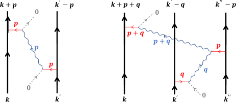
Figure 1: Leading-order diagrams for the two-body potential $V$ (left) and three-body potential $W$ (right) given by Eqs. (12) and (17). Solid black lines represent impurities, dashed lines represent condensate bosons, thin red lines represent boson-impurity interactions, and blue wavy lines represent bosonic excitations.

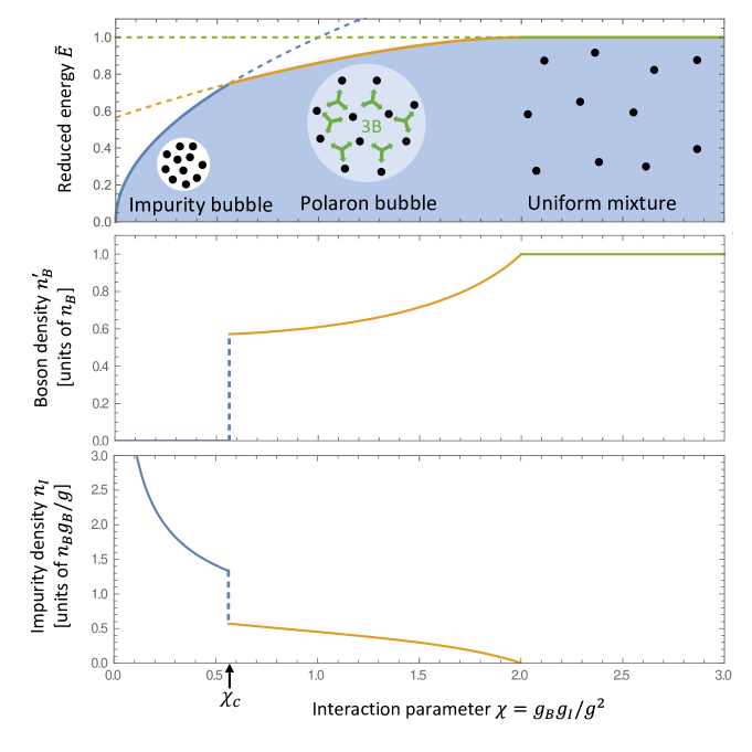
Figure 2: Heavy bosonic impurities immersed in a Bose-Einstein condensate, as a function of the parameter $\chi=g_{B}g_{I}/g^{2}$ characterising the relative strength of repulsion $g$ between impurities and bosons, with respect to the self-repulsions $g_{B}$ and $g_{I}$ of bosons and impurities. There are three distinct phases: impurity bubble, polaron bubble, and uniform mixture. Top panel: energy of the system, along with a schematic representation of the phases - the black dots represent impurities and the blue shading represents the density of the bosonic medium. Middle panel: density of bosons in-between impurities. Lower panel: density of impurities.

Let us consider an interaction $U(\bm{k})$ that becomes negligible for $k\gtrsim\Lambda$. If the range $\Lambda^{-1}$ is much smaller than the coherence length of the bosons $\xi=(8\pi n_{0}a_{B})^{-1/2}$, then, at distances larger than $\Lambda^{-1}$, one can write $E_{P}$, $V$, and $W$ in real space as follows:

$$E_{P}=\frac{2\pi\hbar^{2}}{m}n_{B}\!\left(a_{1}\!+\!a_{2}\!+\!a_{3}\!+\!\frac{a_{1}^{2}\!+\!2a_{1}a_{2}}{\tilde{\xi}}\!+\!\frac{a_{1}^{3}}{\tilde{\xi}^{2}}\right)$$ (18)

$$\tilde{V}(\bm{r})=\frac{4\pi\hbar^{2}}{m}n_{B}\Big{(}-\frac{a_{1}^{2}+2a_{1}a_{2}}{\tilde{\xi}}f(r)+\frac{a_{1}^{3}}{\tilde{\xi}^{2}}f(r)^{2}\Big{)}$$ (19)

$$\tilde{W}(\bm{x},\bm{y})=\frac{4\pi\hbar^{2}}{m}n_{B}\frac{a_{1}^{3}}{\tilde{\xi}^{2}}\Big{(}f(z)f(y)+f(x)f(y)+f(z)f(x)\Big{)}$$ (20)

where $\tilde{\xi}=\xi/\sqrt{2}$, $z=|\bm{x}-\bm{y}|$, and $f(r)=(r/\tilde{\xi})^{-1}\exp(-r/\tilde{\xi})$.

The above expressions are of course not applicable to non-Born interactions such as contact interactions ($\Lambda\to\infty$, for which $a_{1},a_{2},a_{3}\to 0$). One can nevertheless easily generalise these expressions to the case of non-Born interactions, by completing the first terms of the Born expansion of $a$ (i.e. performing the summation of ladder diagrams in the language of perturbation theory). One arrives at:

$$E_{P} =\frac{2\pi\hbar^{2}}{m}n_{B}a\left(1+a/\tilde{\xi}+(a/\tilde{\xi})^{2}\right)$$ (21)

$$\tilde{V}(\bm{r}) =\frac{4\pi\hbar^{2}}{m}n_{B}a\Big{(}-(a/\tilde{\xi})f(r)+(a/\tilde{\xi})^{2}f(r)^{2}\Big{)}$$ (22)

$$\tilde{W}(\bm{x},\bm{y}) =\frac{4\pi\hbar^{2}}{m}n_{B}\frac{a^{3}}{\tilde{\xi}^{2}}\Big{(}f(z)f(y)+f(x)f(y)+f(z)f(x)\Big{)}$$ (23)

It can be checked that Eq. (21) is indeed consistent with the result $E_{P}=\frac{2\pi\hbar^{2}}{m}n_{B}a(1-\sqrt{2}a/\xi)^{-1}$ obtained by the coherent ansatz of Ref. [47] and to second order in $a$ with the diagrammatic result of Ref. [39]. In the rest of this paper, we will restrict our consideration to the low-density limit $\Lambda^{-1},a\ll\xi$, which gives identical results for both Born and non-Born interactions. In this situation, the term proportional to $f(r)^{2}$ in the two-body potential of Eqs. (19) and (22) becomes negligible, and one retrieves the well-known Yukawa attraction mediated between two impurities by a bosonic medium [74, 12, 75, 57, 58].

3 Mean-field theory

An important observation is that the three-body potential, being of third order in $a$, can be either attractive or repulsive depending of the sign of $a$, whereas the two-body potential, being of second order, is always attractive irrespective of the sign of $a$. In the case of a repulsive interaction $a>0$, there is therefore a competition between the induced two-body attraction and three-body repulsion. In this situation, it is tempting to think to that this competition could stabilise the impurities into a liquid state of a certain density [80]. However, this is possible only if the impurities remain mixed with the bosonic medium. On the contrary, the repulsion between the impurities and the bosons tends to separate them, reducing the strength of the mediated interactions.

To understand this interplay, let us consider the case of bosonic impurities. So far we have obtained an essentially exact form of the Hamiltonian in a state corresponding to the vacuum of Fröhlich quasiparticles. The wave function for the impurities remains to be specified to obtain a variational ansatz for the Hamiltonian. Let us choose the Hartree-Fock ansatz in which all the $N_{I}$ impurities occupy the $\bm{k}=\bm{0}$ mode. In this state, the Hamiltonian of Eq. (14) gives the following mean-field energy:

$$E =\frac{1}{2}g_{B}Vn_{B}^{2}+gn_{B}N_{I}+\frac{g_{I}+g_{\text{2}}}{2V}N_{I}^{2}+\frac{g_{\text{3}}}{6V^{2}}N_{I}^{3}$$ (24)

where $g_{B}=U_{B}(\bm{0})$, $g=U(\bm{0})$, $g_{I}=U_{I}(\bm{0})$, $g_{2}=V(\bm{0})=-g^{2}/g_{B}$ and $g_{3}=W(\bm{0},\bm{0})=3g^{3}/(2g_{B}^{2}n_{B})$ represent the low-energy coupling constants of the system. In contrast, the usual mean-field theory, on which previous theoretical works [7, 8, 9, 10, 11, 12] are based, is obtained by taking a Hartree-Fock ansatz for the original Hamiltonian (1), resulting in Eq. (24) with $g_{2}=g_{3}=0$. As we shall see, the mean-field energy of Eq. (24) can give a lower variational upper bound of the exact ground-state energy.

It should be noted that within the Hartree-Fock ansatz, the coupling constants $g_{2}$ and $g_{3}$ are obtained in the Born approximation. However, the induced two- and three-body interactions $V$ and $W$ may or may not be perturbative, depending on the density of the bosons $n_{B}$ and the mass $M$ of the impurities. The Born expansion of $g_{2}$ and $g_{3}$ reads:

$$g_{2} =V(\bm{0})-\frac{1}{V}\sum_{\bm{p}}\frac{V(\bm{p})^{2}}{\frac{\hbar^{2}p^{2}}{M}}+\dots$$

$$=-\frac{\pi\hbar^{2}}{m}\frac{a^{2}}{a_{B}}-\frac{\pi\hbar^{2}}{2m}\frac{M}{m}a^{4}\sqrt{\frac{n_{B}\pi}{a_{B}^{3}}}+\dots$$ (25)

$$g_{3} =W(\bm{0},\bm{0})-\frac{1}{V^{2}}\sum_{\bm{k},\bm{p}}\frac{W(\bm{k},\bm{p})^{2}}{\frac{\hbar^{2}}{M}(\bm{k}+\bm{p}/2)^{2}+\frac{3\hbar^{2}}{4M}p^{2}}+\dots$$

$$=\frac{\pi\hbar^{2}}{m}\frac{3a^{3}}{4n_{B}a_{B}^{2}}-\frac{\hbar^{2}}{m}\frac{M}{m}\frac{a^{6}}{a_{B}^{2}}\underbrace{\lambda}_{17.5755}+\dots$$ (26)

For the two-body and three-body potentials to satisfy the Born approximation, it is thus required that

$$\alpha_{\text{2}}\equiv\frac{M}{m}\frac{1}{2}\sqrt{\frac{\pi a^{4}n_{B}}{a_{B}}}\ll 1\;\text{ and }\;\alpha_{\text{3}}\equiv\frac{4}{3}\lambda\frac{M}{m}n_{B}a^{3}\ll 1.$$ (27)

In addition to these requirements, the validity of the above mean-field energy is limited by the two-body and three-body diluteness conditions,

$$\lambda_{\text{2}}\equiv n_{I}\left(L_{\text{2}}\right)^{3}\ll 1\quad\text{ and }\quad\lambda_{\text{3}}\equiv n_{I}(L_{\text{3}})^{3}\ll 1$$ (28)

where $n_{I}=N_{I}/V$ is the density of impurities, $L_{2}=(g_{I}+g_{2})/(4\pi\hbar^{2}/M)$ is the effective impurity two-body scattering length, and $L_{\text{3}}=[g_{3}/(4\pi\hbar^{2}/M)]^{1/4}$ is the three-body interaction length. In any case, however, the variational nature of the mean-field energy Eq. (24) ensures that it remains an upper bound of the exact ground-state energy.

The mean-field energy Eq. (24) has been written assuming that the whole system is homogeneous. This discards the possibility of the impurities forming a separate phase. We thus need to make a more general ansatz, in which the $N_{I}$ impurities occupy a volume $V^{\prime}$ within the total volume $V$. Among the total number of bosons $N_{B}$, a certain number $N_{B}^{\prime}$ may permeate in-between the impurities inside the volume $V^{\prime}$, forming a density $n_{B}^{\prime}=N_{B}^{\prime}/V^{\prime}$. Let us define the reduced energy $\tilde{E}=(E-\frac{1}{2}g_{B}Vn_{B}^{2})/(gn_{B}N_{I})$ as the energy difference between the total energy $E$ and the energy of the pure homogeneous Bose gas of density $n_{B}$, normalised by the interaction energy $gn_{B}N_{I}$. In the limit of large volume $V$, the reduced energy of the completely segregated phase containing a pure bubble of impurities ($n_{B}^{\prime}=0$) is simply:

$$\tilde{E}_{\text{pure}}=\frac{1}{2}v+\chi\frac{1}{2v}$$ (29)

where $v=\frac{g_{B}n_{B}V^{\prime}}{gN_{I}}$ is a reduced volume and $\chi=\frac{g_{I}g_{B}}{g^{2}}$ is a parameter characterising the relative strengths of interactions. One can easily find the minimum $\tilde{E}_{\text{pure}}=\sqrt{\chi}$ at $v=\sqrt{\chi}$ [10]. On the other hand, in the mixed phase $n_{B}^{\prime}=fn_{B}$ where there is inside the impurity volume $V^{\prime}$ a nonzero fraction $f$ of the outside boson density, the reduced energy is given by:

$$\tilde{E}_{\text{mixed}}=\frac{1}{2}v(1-f)^{2}+f+\frac{1}{2v}(\chi-1)+\frac{1}{4v^{2}f}$$ (30)

For $\chi\geq 2$, minimising this energy with respect to $f$ and $v$ gives $\tilde{E}_{\text{mixed}}=1$, with $f=1$ and $v\to\infty$, corresponding to a completely mixed phase where impurities spread into the condensate and form a uniform mixture. For $\chi<2$, however, a non trivial solution of finite volume is found corresponding to a bubble of polarons, i.e. impurities mixed with bosons. This bubble has a lower energy than a pure bubble of impurities because of the induced two-body attraction. Moreover, its stability results from the equilibrium between the induced three-body repulsion and the pressure from the outside bosons. At the particular value $\chi=1$, the induced two-body interaction exactly cancels the effects of the direct repulsion between impurities, and the polarons form a Bose gas interacting only with three-body interactions. Finally, at the critical value $\chi_{c}=9/16=0.5625$, the energy of the polaron bubble becomes equal to $\tilde{E}_{\text{pure}}$. At this point, it is energetically more favourable for the polarons to collapse into a bubble of impurities devoid of any bosons, about twice smaller than the polaron bubble. This scenario is represented in Fig. 2.

It should be noted that in this simple mean-field theory, the kinetic energies of the bosons and impurities are neglected and densities are assumed to be uniform inside and outside the volume $V^{\prime}$. Taking into account the kinetic energies would smooth the densities near the bubble surface and add a small surface tension that would determine the bubble’s geometry - a sphere in the present case of a homogeneous Bose gas. Apart from these effects, the kinetic energies may be neglected for a sufficiently large number of impurities. Indeed, the contribution of the kinetic energies to $\tilde{E}$ is of the order of $A_{B}=(N_{I}4\pi a/\xi)^{-1}$. Although $a/\xi$ is assumed to be small, a mesoscopic number of impurities can easily make $A_{B}\ll 1$.

It is also worthwhile to point out that in this limit, the polaron bubble cannot exist as a metastable state for $\chi\leq\chi_{c}$. Indeed, the activation energy for any local fluctuation in the polaron bubble to nucleate a region free of bosons is solely due to the kinetic energy cost of reducing the density of bosons to zero in that region, which is proportional to $A_{B}$. For $A_{B}\ll 1$, there is therefore almost no energy cost, and the polaron bubble should quickly collapse to an impurity bubble. The smallness of $A_{B}$ is also required to guarantee that the range $\xi/\sqrt{f}$ of mediated interactions remains smaller than the average spacing between the impurities.

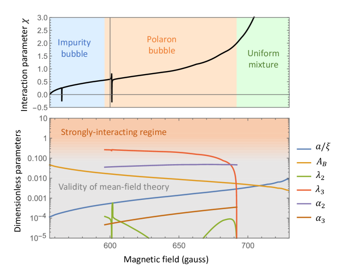
Figure 3: Expected phases of caesium-133 atoms immersed in a condensate of lithium-7 atoms, as a function of applied magnetic field. Top panel: interaction parameter $\chi=g_{I}g_{B}/g^{2}$. Bottom panel: various dimensionless parameters [see Eqs. (27) and (28)] characterizing the validity of the Hartree-Fock ansatz for a dilute system, obtained for a total number of caesium atoms $N_{I}\sim 10^{5}$ and a density of lithium atoms $n_{B}\sim 10^{12}\text{ cm}^{-3}$.

4 Ultracold atomic mixtures

Finally, let us consider how this physics could be observed with ultracold atoms. The basic requirements are a mixture of heavy and light atoms (for instance $m/M=0.05$) and a small ratio $a/\xi$ (for instance 0.0001). One should then specify the ratio $g_{B}/g$. A small ratio ensures that the impurities remain a minority among the bosons (for instance $g_{B}/g=0.2$, giving $n_{I}\approx 0.2n_{B}^{\prime}$). Near the three-body-dominated regime $\chi\approx 1$ ($v\approx 2$,$f\approx 0.6$), these values lead to the boson diluteness parameter $n_{B}a_{B}^{3}\approx 4\times 10^{-12}$, the impurity 2-body and 3-body diluteness parameters $\lambda_{2}\approx 5\times 10^{-5}(\chi-1)^{3}$ and $\lambda_{3}\approx 0.1$. The Born conditions of Eq. (27) are also satisfied with $\alpha_{\text{2B}}\approx 3\times 10^{-3}$ and $\alpha_{\text{3B}}\approx 2\times 10^{-6}$. Taking a typical condensate density $n_{B}=10^{15}\,\text{cm}^{-3}$, and the lightest boson available (lithium-7), one finds $a_{B}\approx 0.3a_{0}$, $a\approx 3a_{0}$, and $a_{I}\approx 150a_{0}$, where $a_{0}$ designates the Bohr radius $a_{0}\approx 5.29\,\times\>10^{-11}$ m. These are moderate values of atomic scattering lengths, for which atomic losses should remain small. Requiring $A_{B}$ to be smaller than $0.01$ sets the number of impurities to $\sim 10^{6}$, which also corresponds to a realistic number. The formation of a bubble could be observed by imaging the impurity density, as in previous experiments, and the transition from the impurity bubble to the polaron bubble could be evidenced by probing the change of boson density inside the bubble, for instance by shining a light causing inelastic collisions between bosons and impurities.

It should be pointed out that the energy difference $\Delta=(E_{\text{mixed}}-E_{\text{pure}})/N_{I}$ between the polaron bubble and the impurity bubble is only about 14 nK near $\chi\approx 1$. Although it would seem that a very low temperature $k_{B}T\ll\Delta$ is needed to observe the two phases distinctly, previous experiments [3, 5] have shown that such tiny interaction energies are enough to drive observable transitions even at temperatures of the order of 100 nK. Interestingly, it is possible to increase the energy difference by considering a higher ratio $a/\xi$, for instance $a/\xi=$0.01, giving $\Delta\approx 300$ nK. In this case, the polaron bubble becomes strongly interacting with $\lambda_{2}\approx 0.5(\chi-1)^{3}$ and $\lambda_{3}\approx 1.0$, along with $\alpha_{2}\approx 0.35$ and $\alpha_{3}\approx 0.02$. Although the mean-field theory is not quantitative any more in this regime, its variational nature indicates that a dense bubble of polarons dominated by strong three-body interactions should exist near $\chi=1$. These strong three-body interactions may indeed overcome the inelastic three-body processes naturally occurring in ultracold atomic clouds. To account for these inelastic processes, the three-body coupling constant $g_{3}$ may be generalised to a complex number $(4\pi\hbar^{2}/M)\times(L_{3}^{4}-i\mathcal{L}_{3}^{4})$. Since all scattering lengths $a_{B}$, $a$, and $L_{2}$ remain small near $\chi=1$, the three-body loss rates $K=(h/M)\mathcal{L}_{3}^{4}$ should take an off-resonant value, typically $\sim 10^{-28}\,\text{cm}^{6}\text{s}^{-1}$ [12], corresponding to $\mathcal{L}_{3}\sim 10\,\text{nm}$. On the other hand, $L_{3}\sim 100\text{ nm},$ which shows that elastic three-body collisions may dominate inelastic ones in this regime.

As a concrete illustration, the expected phases of a mixture of lithium-7 and caesium-133 atoms (in their respective ground hyperfine states) are shown in Fig. 3, as a function of applied magnetic field. The figure is obtained for $N_{I}=10^{5}$ caesium atoms, and a lithium density $n_{B}\sim 10^{12}\text{ cm}^{-3}$. The interaction parameter $\chi=g_{I}g_{B}/g^{2}$ is obtained from the scattering lengths data for caesium-133 [81], lithium-7 [82], and caesium-133 – lithium-7 [83]. The polaron bubble phase is expected in a 100 gauss-wide window. Even for the relatively low density considered, the polaron bubble appears to be dense with respect to the induced three-body interactions, with $\lambda_{\text{3}}$ approaching unity.

5 Conclusion

In summary, it has been shown that mixtures of bosons with repulsive interactions may not only fully mix or fully separate, but also form polaron bubbles. In contrast to usual dilute gases, these polaron bubbles can be rather dense and dominated by three-body interactions. These bubbles therefore provide a unique setting in the context of ultracold atomic gases to study strongly-interacting gases with elastic three-body interactions, a situation that has been so far out of experimental reach.

 

The author would like to thank Hiroyuki Tajima, Shimpei Endo, Ludovic Pricoupenko, Munekazu Horikoshi, Tetsuo Hatsuda, and Yoshiro Takahashi for useful discussions. The author is also grateful to Paul Julienne for providing the caesium scattering length data. This work was supported by the RIKEN Incentive Research Project and JSPS Grants-in-Aid for Scientific Research on Innovative Areas (No. JP18H05407).

References

- [1] G. K. Walters and W. M. Fairbank, “Phase Separation in — Solutions” Phys. Rev., 103, 262–263, Jul 1956.
- [2] E. H. Graf, D. M. Lee, and J. D. Reppy, “Phase Separation and the Superfluid Transition in Liquid - Mixtures” Phys. Rev. Lett., 19, 417–419, Aug 1967.
- [3] J. Stenger, S. Inouye, D. M. Stamper-Kurn, H.-J. Miesner, A. P. Chikkatur, and W. Ketterle, “Spin domains in ground-state Bose-Einstein condensates” Nature, 396, 345–348, 1998.
- [4] G. Modugno, M. Modugno, F. Riboli, G. Roati, and M. Inguscio, “Two Atomic Species Superfluid” Phys. Rev. Lett., 89, 190404, Oct 2002.
- [5] S. B. Papp, J. M. Pino, and C. E. Wieman, “Tunable Miscibility in a Dual-Species Bose-Einstein Condensate” Phys. Rev. Lett., 101, 040402, Jul 2008.
- [6] K. L. Lee, N. B. Jørgensen, L. J. Wacker, M. G. Skou, K. T. Skalmstang, J. J. Arlt, and N. P. Proukakis, “Time-of-flight expansion of binary Bose–Einstein condensates at finite temperature” New Journal of Physics, 20, 053004, may 2018.
- [7] B. D. Esry, C. H. Greene, J. P. Burke, Jr., and J. L. Bohn, “Hartree-Fock Theory for Double Condensates” Phys. Rev. Lett., 78, 3594–3597, May 1997.
- [8] H. Pu and N. P. Bigelow, “Properties of Two-Species Bose Condensates” Phys. Rev. Lett., 80, 1130–1133, Feb 1998.
- [9] E. Timmermans, “Phase Separation of Bose-Einstein Condensates” Phys. Rev. Lett., 81, 5718–5721, Dec 1998.
- [10] P. Ao and S. T. Chui, “Binary Bose-Einstein condensate mixtures in weakly and strongly segregated phases” Phys. Rev. A, 58, 4836–4840, Dec 1998.
- [11] M. Trippenbach, K. Góral, K. Rzazewski, B. Malomed, and Y. B. Band, “Structure of binary Bose-Einstein condensates” J. Phys. B, 33, 4017–4031, sep 2000.
- [12] H. S. C. J. Pethick, Bose-Einstein Condensation in Dilute Gases . Cambridge University Press, 2002.
- [13] C. R. Cabrera, L. Tanzi, J. Sanz, B. Naylor, P. Thomas, P. Cheiney, and L. Tarruell, “Quantum liquid droplets in a mixture of Bose-Einstein condensates” Science, 359, 301–304, 2018.
- [14] P. Cheiney, C. R. Cabrera, J. Sanz, B. Naylor, L. Tanzi, and L. Tarruell, “Bright Soliton to Quantum Droplet Transition in a Mixture of Bose-Einstein Condensates” Phys. Rev. Lett., 120, 135301, Mar 2018.
- [15] G. Semeghini, G. Ferioli, L. Masi, C. Mazzinghi, L. Wolswijk, F. Minardi, M. Modugno, G. Modugno, M. Inguscio, and M. Fattori, “Self-Bound Quantum Droplets of Atomic Mixtures in Free Space” Phys. Rev. Lett., 120, 235301, Jun 2018.
- [16] D. S. Petrov, “Quantum Mechanical Stabilization of a Collapsing Bose-Bose Mixture” Phys. Rev. Lett., 115, 155302, Oct 2015.
- [17] A. Schirotzek, C.-H. Wu, A. Sommer, and M. W. Zwierlein, “Observation of Fermi Polarons in a Tunable Fermi Liquid of Ultracold Atoms” Phys. Rev. Lett., 102, 230402, Jun 2009.
- [18] S. Nascimbène, N. Navon, K. J. Jiang, L. Tarruell, M. Teichmann, J. McKeever, F. Chevy, and C. Salomon, “Collective Oscillations of an Imbalanced Fermi Gas: Axial Compression Modes and Polaron Effective Mass” Phys. Rev. Lett., 103, 170402, Oct 2009.
- [19] M. Koschorreck, D. Pertot, E. Vogt, B. Fröhlich, M. Feld, and M. Köhl, “Attractive and repulsive Fermi polarons in two dimension” Nature, 485, 619–622, 2012.
- [20] C. Kohstall, M. Zaccanti, M. Jag, A. Trenkwalder, P. Massignan, G. M. Bruun, F. Schreck, and R. Grimm, “Metastability and coherence of repulsive polarons in a strongly interacting Fermi mixture” Nature, 485, 615–618, May 2012.
- [21] M. Cetina, M. Jag, R. S. Lous, I. Fritsche, J. T. M. Walraven, R. Grimm, J. Levinsen, M. M. Parish, R. Schmidt, M. Knap, and E. Demler, “Ultrafast many-body interferometry of impurities coupled to a Fermi sea” Science, 354, 96–99, 2016.
- [22] F. Scazza, G. Valtolina, P. Massignan, A. Recati, A. Amico, A. Burchianti, C. Fort, M. Inguscio, M. Zaccanti, and G. Roati, “Repulsive Fermi Polarons in a Resonant Mixture of Ultracold Atoms” Phys. Rev. Lett., 118, 083602, Feb 2017.
- [23] Z. Yan, P. B. Patel, B. Mukherjee, R. J. Fletcher, J. Struck, and M. W. Zwierlein, “Boiling a Unitary Fermi Liquid” Phys. Rev. Lett., 122, 093401, Mar 2019.
- [24] J. Catani, G. Lamporesi, D. Naik, M. Gring, M. Inguscio, F. Minardi, A. Kantian, and T. Giamarchi, “Quantum dynamics of impurities in a one-dimensional Bose gas” Phys. Rev. A, 85, 023623, Feb 2012.
- [25] J. W. Park, C.-H. Wu, I. Santiago, T. G. Tiecke, S. Will, P. Ahmadi, and M. W. Zwierlein, “Quantum degenerate Bose-Fermi mixture of chemically different atomic species with widely tunable interactions” Phys. Rev. A, 85, 051602, May 2012.
- [26] M.-G. Hu, M. J. Van de Graaff, D. Kedar, J. P. Corson, E. A. Cornell, and D. S. Jin, “Bose Polarons in the Strongly Interacting Regime” Phys. Rev. Lett., 117, 055301, Jul 2016.
- [27] N. B. Jørgensen, L. Wacker, K. T. Skalmstang, M. M. Parish, J. Levinsen, R. S. Christensen, G. M. Bruun, and J. J. Arlt, “Observation of Attractive and Repulsive Polarons in a Bose-Einstein Condensate” Phys. Rev. Lett., 117, 055302, Jul 2016.
- [28] B. J. DeSalvo, K. Patel, J. Johansen, and C. Chin, “Observation of a Degenerate Fermi Gas Trapped by a Bose-Einstein Condensate” Phys. Rev. Lett., 119, 233401, Dec 2017.
- [29] F. Camargo, R. Schmidt, J. D. Whalen, R. Ding, G. Woehl, S. Yoshida, J. Burgdörfer, F. B. Dunning, H. R. Sadeghpour, E. Demler, and T. C. Killian, “Creation of Rydberg Polarons in a Bose Gas” Phys. Rev. Lett., 120, 083401, Feb 2018.
- [30] Z. Z. Yan, Y. Ni, C. Robens, and M. W. Zwierlein, “Bose polarons near quantum criticality” arXiv:1904.02685, 2019.
- [31] F. Chevy, “Universal phase diagram of a strongly interacting Fermi gas with unbalanced spin populations” Phys. Rev. A, 74, 063628, Dec 2006.
- [32] N. Prokof’ev and B. Svistunov, “Fermi-polaron problem: Diagrammatic Monte Carlo method for divergent sign-alternating series” Phys. Rev. B, 77, 020408, Jan 2008.
- [33] P. Massignan, M. Zaccanti, and G. M. Bruun, “Polarons, dressed molecules and itinerant ferromagnetism in ultracold Fermi gases” Reports on Progress in Physics, 77, 034401, feb 2014.
- [34] R. Schmidt, M. Knap, D. A. Ivanov, J.-S. You, M. Cetina, and E. Demler, “Universal many-body response of heavy impurities coupled to a Fermi sea: a review of recent progress” Reports on Progress in Physics, 81, 024401, jan 2018.
- [35] R. M. Kalas and D. Blume, “Interaction-induced localization of an impurity in a trapped Bose-Einstein condensate” Phys. Rev. A, 73, 043608, Apr 2006.
- [36] F. M. Cucchietti and E. Timmermans, “Strong-Coupling Polarons in Dilute Gas Bose-Einstein Condensates” Phys. Rev. Lett., 96, 210401, Jun 2006.
- [37] J. Tempere, W. Casteels, M. K. Oberthaler, S. Knoop, E. Timmermans, and J. T. Devreese, “Feynman path-integral treatment of the BEC-impurity polaron” Phys. Rev. B, 80, 184504, Nov 2009.
- [38] S. P. Rath and R. Schmidt, “Field-theoretical study of the Bose polaron” Phys. Rev. A, 88, 053632, Nov 2013.
- [39] R. S. Christensen, J. Levinsen, and G. M. Bruun, “Quasiparticle Properties of a Mobile Impurity in a Bose-Einstein Condensate” Phys. Rev. Lett., 115, 160401, Oct 2015.
- [40] A. G. Volosniev, H.-W. Hammer, and N. T. Zinner, “Real-time dynamics of an impurity in an ideal Bose gas in a trap” Phys. Rev. A, 92, 023623, Aug 2015.
- [41] F. Grusdt, Y. E. Shchadilova, A. N. Rubtsov, and E. Demler, “Renormalization group approach to the Fröhlich polaron model: application to impurity-BEC problem” Scientific Reports, 5, 12124, 2015.
- [42] J. Vlietinck, W. Casteels, K. V. Houcke, J. Tempere, J. Ryckebusch, and J. T. Devreese, “Diagrammatic Monte Carlo study of the acoustic and the Bose-Einstein condensate polaron” New Journal of Physics, 17, 033023, 2015.
- [43] L. A. Peña Ardila and S. Giorgini, “Impurity in a Bose-Einstein condensate: Study of the attractive and repulsive branch using quantum Monte Carlo methods” Phys. Rev. A, 92, 033612, Sep 2015.
- [44] L. A. P. n. Ardila and S. Giorgini, “Bose polaron problem: Effect of mass imbalance on binding energy” Phys. Rev. A, 94, 063640, Dec 2016.
- [45] F. Grusdt and M. Fleischhauer, “Tunable Polarons of Slow-Light Polaritons in a Two-Dimensional Bose-Einstein Condensate” Phys. Rev. Lett., 116, 053602, Feb 2016.
- [46] E. Nakano and H. Yabu, “BEC-polaron gas in a boson-fermion mixture: A many-body extension of Lee-Low-Pines theory” Phys. Rev. B, 93, 205144, May 2016.
- [47] Y. E. Shchadilova, R. Schmidt, F. Grusdt, and E. Demler, “Quantum Dynamics of Ultracold Bose Polarons” Phys. Rev. Lett., 117, 113002, Sep 2016.
- [48] S. M. Yoshida, S. Endo, J. Levinsen, and M. M. Parish, “Universality of an Impurity in a Bose-Einstein Condensate” Phys. Rev. X, 8, 011024, Feb 2018.
- [49] J. Levinsen, M. M. Parish, R. S. Christensen, J. J. Arlt, and G. M. Bruun, “Finite-temperature behavior of the Bose polaron” Phys. Rev. A, 96, 063622, Dec 2017.
- [50] L. Parisi and S. Giorgini, “Quantum Monte Carlo study of the Bose-polaron problem in a one-dimensional gas with contact interactions” Phys. Rev. A, 95, 023619, Feb 2017.
- [51] M. Sun, H. Zhai, and X. Cui, “Visualizing the Efimov Correlation in Bose Polarons” Phys. Rev. Lett., 119, 013401, Jul 2017.
- [52] A. G. Volosniev and H.-W. Hammer, “Analytical approach to the Bose-polaron problem in one dimension” Phys. Rev. A, 96, 031601, Sep 2017.
- [53] F. Grusdt, G. E. Astrakharchik, and E. A. Demler, “Bose polarons in ultracold atoms in one dimension: beyond the Fröhlich paradigm” New Journal of Physics, 19, 103035, 2017.
- [54] A. Lampo, S. H. Lim, M. Ángel García-March, , and M. Lewenstein, “Bose polaron as an instance of quantum Brownian motion” Quantum, 1, 30, 2017.
- [55] N. J. S. Loft, Z. Wu, and G. M. Bruun, “Mixed-dimensional Bose polaron” Phys. Rev. A, 96, 033625, Sep 2017.
- [56] M. Sun and X. Cui, “Enhancing the Efimov correlation in Bose polarons with large mass imbalance” Phys. Rev. A, 96, 022707, Aug 2017.
- [57] P. Naidon, “Two Impurities in a Bose-Einstein Condensate: From Yukawa to Efimov Attracted Polarons” J. Phys. Soc. Jpn., 87, 043002, 2018.
- [58] A. Camacho-Guardian, L. A. Peña Ardila, T. Pohl, and G. M. Bruun, “Bipolarons in a Bose-Einstein Condensate” Phys. Rev. Lett., 121, 013401, Jul 2018.
- [59] N.-E. Guenther, P. Massignan, M. Lewenstein, and G. M. Bruun, “Bose Polarons at Finite Temperature and Strong Coupling” Phys. Rev. Lett., 120, 050405, Feb 2018.
- [60] F. Grusdt, K. Seetharam, Y. Shchadilova, and E. Demler, “Strong-coupling Bose polarons out of equilibrium: Dynamical renormalization-group approach” Phys. Rev. A, 97, 033612, Mar 2018.
- [61] V. Pastukhov, “Polaron in dilute 2D Bose gas at low temperatures” J. Phys. B, 51, 155203, jul 2018.
- [62] A. Lampo, C. Charalambous, M. A. García-March, and M. Lewenstein, “Non-Markovian polaron dynamics in a trapped Bose-Einstein condensate” Phys. Rev. A, 98, 063630, Dec 2018.
- [63] C. Charalambous, M. Garcia-March, A. Lampo, M. Mehboudi, and M. Lewenstein, “Two distinguishable impurities in BEC: squeezing and entanglement of two Bose polarons” SciPost Phys., 6, 10, 2019.
- [64] M. Mehboudi, A. Lampo, C. Charalambous, L. A. Correa, M. A. García-March, and M. Lewenstein, “Using Polarons for sub-nK Quantum Nondemolition Thermometry in a Bose-Einstein Condensate” Phys. Rev. Lett., 122, 030403, Jan 2019.
- [65] B. Kain and H. Y. Ling, “Analytical study of static beyond-Fröhlich Bose polarons in one dimension” Phys. Rev. A, 98, 033610, Sep 2018.
- [66] S. Van Loon, W. Casteels, and J. Tempere, “Ground-state properties of interacting Bose polarons” Phys. Rev. A, 98, 063631, Dec 2018.
- [67] M. Drescher, M. Salmhofer, and T. Enss, “Real-space dynamics of attractive and repulsive polarons in Bose-Einstein condensates” Phys. Rev. A, 99, 023601, Feb 2019.
- [68] S. I. Mistakidis, G. C. Katsimiga, G. M. Koutentakis, T. Busch, and P. Schmelcher, “Quench Dynamics and Orthogonality Catastrophe of Bose Polarons” Phys. Rev. Lett., 122, 183001, May 2019.
- [69] K. Watanabe, E. Nakano, and H. Yabu, “Bose polaron in spherically symmetric trap potentials: Ground states with zero and lower angular momenta” Phys. Rev. A, 99, 033624, Mar 2019.
- [70] G. Panochko and V. Pastukhov, “Mean-field construction for spectrum of one-dimensional Bose polaron” Annals of Physics, 409, 167933, 2019.
- [71] J. Takahashi, R. Imai, E. Nakano, and K. Iida, “Bose polaron in spherical trap potentials: Spatial structure and quantum depletion” Phys. Rev. A, 100, 023624, Aug 2019.
- [72] T. Ichmoukhamedov and J. Tempere, “Feynman path-integral treatment of the Bose polaron beyond the Fröhlich model” Phys. Rev. A, 100, 043605, Oct 2019.
- [73] D. Boyanovsky, D. Jasnow, X.-L. Wu, and R. C. Coalson, “Dynamics of relaxation and dressing of a quenched Bose polaron” Phys. Rev. A, 100, 043617, Oct 2019.
- [74] J. Bardeen, G. Baym, and D. Pines, “Effective Interaction of Atoms in Dilute Solutions of in at Low Temperatures” Phys. Rev., 156, 207–221, Apr 1967.
- [75] Z. Yu and C. J. Pethick, “Induced interactions in dilute atomic gases and liquid helium mixtures” Phys. Rev. A, 85, 063616, Jun 2012.
- [76] R. G. Newton, Scattering Theory of Waves and Particles. Dover Publications, 2013.
- [77] N. N. Bogoliubov, “On the theory of superfluidity,” J. Phys. (USSR), 11, 23, 1947.
- [78] H. Fröhlich, “Electrons in lattice fields,” Advances in Physics, 3, 325–361, July. 1954.
- [79] J. T. Devreese and A. S. Alexandrov, “Frölich polaron and bipolaron: recent developments” Reports on Progress in Physics, 72, 066501, 2009.
- [80] A. Bulgac, “Dilute Quantum Droplets” Phys. Rev. Lett., 89, 050402, Jul 2002.
- [81] M. Berninger, A. Zenesini, B. Huang, W. Harm, H.-C. Nägerl, F. Ferlaino, R. Grimm, P. S. Julienne, and J. M. Hutson, “Feshbach resonances, weakly bound molecular states, and coupled-channel potentials for cesium at high magnetic fields” Phys. Rev. A, 87, 032517, Mar 2013.
- [82] S. E. Pollack, D. Dries, M. Junker, Y. P. Chen, T. A. Corcovilos, and R. G. Hulet, “Extreme Tunability of Interactions in a Bose-Einstein Condensate” Phys. Rev. Lett., 102, 090402, Mar 2009.
- [83] P. Naidon, “Magnetic Feshbach resonances in mixtures” arXiv:2001.05329, 2020.