Fermi liquid theory for nonlinear transport through a multilevel Anderson impurity

Abstract

We present a microscopic Fermi-liquid view on the low-energy transport through an Anderson impurity with $N$ discrete levels, at arbitrary electron filling $N_{d}$. It is applied to nonequilibrium current fluctuations, for which the two-quasiparticle collision integral and the three-body correlations that determine the quasiparticle energy shift play important roles. Using the numerical renormalization group up to $N=6$, we find that for strong interactions the three-body fluctuations are determined by a single parameter other than the Kondo energy scale in a wide filling range $1\lesssim N_{d}\lesssim N-1$. It significantly affects the current noise for $N>2$ and the behavior of noise in magnetic fields.

Introduction.— Highly correlated low-energy states of the Kondo systems show fascinating universal behavior Hewson (1993), which can be described by a Fermi liquid (FL) theory in zero dimension Wilson (1975); Nozières (1974); Yamada (1975); Shiba (1975); Yoshimori (1976). FL behaviors have been observed for the nonlinear current through quantum dots Grobis et al. (2008); Scott et al. (2009) and also the current noise Zarchin et al. (2008); Delattre et al. (2009); Yamauchi et al. (2011); Ferrier et al. (2016) which is now one of the most important probes to explore quantum states. Furthermore, in addition to the spin, internal degrees of freedom such as orbital, flavor, etc., bring an interesting variety in the Kondo effect, occurring in a carbon nanotube Laird et al. (2015); Ferrier et al. (2016) and novel quantum systems such as ultracold atomic gases Ono et al. (2019) and quark matters Yasui and Ozaki (2017).

Transport properties of the local FL have successfully been described by the renormalized quasiparticles and their collisions due to the residual interaction, especially at the symmetric point where both the particle-hole (PH) and time-reversal (TR) symmetries are present Hershfield et al. (1992); Oguri (2001); Aligia (2012); Muñoz et al. (2013). These symmetries are broken in real systems by external fields, such as a gate voltage and a magnetic field. In this case, a single quasiparticle captures the quadratic dependence on frequency $\omega$, temperature $T$, and bias voltage $V$ not only through the well-investigated damping rate but also through the energy shift. It has recently been clarified that the quadratic energy shift is determined by the three-body correlations between the impurity electrons Mora et al. (2015); Filippone et al. (2018); Oguri and Hewson (2018a, b, c). It shows that the three-body correlations are essential parameters for describing the FL transport.

Despite its importance, the current noise Hershfield (1992); Gogolin and Komnik (2006); Sela et al. (2006); Sela and Malecki (2009); Mora et al. (2009); Sakano et al. (2011); Karki et al. (2018) has been still less elucidated away from the symmetric point. A major milestone was achieved by Mora et al Mora et al. (2015), who have extended Nozières phenomenological FL theory Nozières (1974) to give the formula of the nonlinear noise for a PH asymmetric single-orbital Anderson model at zero magnetic field. Further investigation, however, is required to clarify the physics of nonequilibrium fluctuations in the Kondo systems with various internal degrees of freedom.

In this letter, we give a microscopic view on the low-energy transport through a multilevel Anderson impurity for a wide range of electron fillings $N_{d}$. It is described in terms of five FL parameters, which can be calculated using the numerical renormalization group (NRG) Wilson (1975) up to $N=6$. We find that for strong interactions the three-body correlations for $N$ degenerate levels are determined by a single parameter over a wide filling range $1\lesssim N_{d}\lesssim N-1$, which includes the intermediate valence regions. We also provide a current-noise formula for the FL, taking into account all the two-quasiparticle collision processes Pitaevskii and Lifshitz (1981); Haug and Jauho (2008). It satisfies a Ward identity Yamada (1975); Shiba (1975); Yoshimori (1976) for the Keldysh vertex function, and resolves an essential problem of the current conservation of the correlated electrons under a nonequilibrium condition Hershfield et al. (1992); Hershfield (1992). We also calculate the nonlinear noise using the NRG, and demonstrate that the internal degrees of freedom give a wide variety to the filling dependence. We also examine the effect of a magnetic field that breaks the TR symmetry, and show that the noise of a spin-1/2 quantum dot exhibits a universal Kondo scaling behavior.

Model.— We consider an $N$-level Anderson impurity coupled to two leads on the left ($L$) and right ($R$):

$$\!\mathcal{H}\,=\ \sum_{\sigma=1}^{N}\epsilon_{d\sigma}\,n_{d\sigma}\,+\sum_{\lambda=L,R}\sum_{\sigma=1}^{N}v_{\lambda}\left(\psi_{\lambda\sigma}^{\dagger}d_{\sigma}+d_{\sigma}^{{\dagger}}\psi_{\lambda\sigma}\right)$$

$$\quad\ +\sum_{\lambda=L,R}\sum_{\sigma=1}^{N}\int_{-D}^{D}\!d\epsilon\,\epsilon\,c^{\dagger}_{\epsilon\lambda\sigma}c_{\epsilon\lambda\sigma}\,+\frac{U}{2}\sum_{\sigma\neq\sigma^{\prime}}n_{d\sigma}n_{d\sigma^{\prime}}.$$ (1)

$d^{{\dagger}}_{\sigma}$ creates an impurity electron with energy $\epsilon_{d\sigma}$, $n_{d\sigma}\equiv d^{{\dagger}}_{\sigma}d_{\sigma}$, and $U$ the Coulomb repulsion. Conduction electrons are normalized as $\{c^{\phantom{\dagger}}_{\epsilon\lambda\sigma},c^{\dagger}_{\epsilon^{\prime}\lambda^{\prime}\sigma^{\prime}}\}=\delta_{\lambda\lambda^{\prime}}\,\delta_{\sigma\sigma^{\prime}}\delta(\epsilon-\epsilon^{\prime})$. The coupling $v_{\lambda}$ between $\psi_{\lambda\sigma}\equiv\int_{-D}^{D}d\epsilon\sqrt{\rho_{c}}\,c^{\phantom{\dagger}}_{\epsilon\lambda\sigma}$ and $d^{{\dagger}}_{\sigma}$ yields a resonance of the width $\Delta\equiv\Gamma_{L}+\Gamma_{R}$, with $\Gamma_{\lambda}=\pi\rho_{c}v_{\lambda}^{2}$, $\,\,\rho_{c}=1/(2D)$, and $D$ the half band width.

In this work, we study the nonlinear current noise Hershfield (1992)

$$\!\!\!\!S_{\mathrm{noise}}^{\mathrm{QD}}=\!\int_{-\infty}^{\infty}\!\!dt\,\left\langle\delta\widehat{J}(t)\,\delta\widehat{J}(0)+\delta\widehat{J}(0)\,\delta\widehat{J}(t)\right\rangle_{V}\;.$$ (2)

Here, $\delta\widehat{J}(t)\equiv\widehat{J}(t)-\langle\widehat{J}(0)\rangle_{V}$ is the current fluctuation operator through the quantum dot , and $\langle\cdots\rangle_{V}$ is the Keldysh steady-state average defined at finite bias voltages $eV\equiv\mu_{L}-\mu_{R}$ with $\mu_{\lambda}$ the chemical potential for $\lambda=L,R$ . The average current $J\equiv\langle\widehat{J}(0)\rangle_{V}$ is given by Hershfield et al. (1992),

$$J\,=\,\frac{e}{h}\sum_{\sigma}\int_{-\infty}^{\infty}\!\!d\omega\,\bigl{[}\,f_{L}(\omega)-f_{R}(\omega)\,\bigr{]}\,\mathcal{T}_{\sigma}(\omega)\,.$$ (3)

Here, $f_{\lambda}(\omega)\equiv[e^{(\omega-\mu_{\lambda})/T}+1]^{-1}$ the Fermi function, $\mathcal{T}_{\sigma}(\omega)\equiv-\frac{4\Gamma_{L}\Gamma_{R}}{\Gamma_{L}+\Gamma_{R}}\,\mathrm{Im}\,G_{\sigma}^{r}(\omega)$ the transmission probability, and $G_{\sigma}^{r}(\omega)=[\,\omega-\epsilon_{d\sigma}+i\Delta\,-\Sigma_{\sigma}^{r}(\omega)\,]^{-1}$ the retarded Green’s function with $\Sigma_{\sigma}^{r}(\omega)$ the self-energy. From this $\mathcal{T}_{\sigma}(\omega)$, we can also deduce the thermal conductivity $\kappa_{\mathrm{QD}}$ for the heat current $J_{Q}=-\kappa_{\mathrm{QD}}\,\delta T$, induced by the temperature difference $\delta T$ between the two leads Costi and Zlatić (2010).

Fermi-liquid parameters.— We investigate low-energy transport up to next leading order. To this end, we expand $\Sigma_{\sigma}^{r}(\omega)$ up to terms of order $\omega^{2}$, $T^{2}$, and $(eV)^{2}$ for general $N$, extending the latest FL description for spin $1/2$ case Oguri and Hewson (2018a, b). The expansion coefficients play an important role as the FL parameters.

The phase shift $\delta_{\sigma}\equiv\cot^{-1}(\epsilon_{d\sigma}^{*}/\Delta)$ is a parameter of primary importance, with $\epsilon_{d\sigma}^{*}\equiv\epsilon_{d\sigma}+\left.\Sigma_{\sigma}^{r}(0)\right|_{T=eV=0}$ the effective impurity level. It determines the occupation number $\langle n_{d\sigma}\rangle=\delta_{\sigma}/\pi$, and the density of states $\rho_{d\sigma}\equiv{\sin^{2}\delta_{\sigma}}/{(\pi\Delta)}$. The renormalization factor is given by the first derivative $z_{\sigma}\equiv\bigl{[}1-\frac{\partial\Sigma_{\sigma}^{r}(\omega)}{\partial\omega}|_{\omega=0}\bigr{]}^{-1}$, defined at $T=eV=0$. It is also related to the static susceptibility $\chi_{\sigma_{1}\sigma_{2}}\equiv\int_{0}^{1/T}\!\!d\tau\,\left\langle\delta n_{d\sigma_{1}}(\tau)\,\delta n_{d\sigma_{2}}\right\rangle$, as $\chi_{\sigma\sigma}\xrightarrow{T\to 0}\rho_{d\sigma}/z_{\sigma}$, with $\delta n_{d\sigma}\equiv n_{d\sigma}-\langle n_{d\sigma}\rangle$ Yamada (1975); Shiba (1975); Yoshimori (1976). The second derivative is a complex number, the imaginary part of which corresponds to the single-quasiparticle damping rate of order $\omega^{2}$, $T^{2}$, and $(eV)^{2}$ Hershfield et al. (1992); Oguri (2001). The real part corresponds to the quadratic energy shift that is determined by the nonlinear susceptibility defined at equilibrium Oguri and Hewson (2018a, b):

$$\chi_{\sigma_{1}\sigma_{2}\sigma_{3}}^{[3]}\!\equiv -\!\int_{0}^{1/T}\!\!\!\!d\tau_{3}\!\!\int_{0}^{1/T}\!\!\!\!d\tau_{2}\,\langle T_{\tau}\delta n_{d\sigma_{3}}(\tau_{3})\,\delta n_{d\sigma_{2}}(\tau_{2})\,\delta n_{d\sigma_{1}}\rangle\,,$$

with $T_{\tau}$ the imaginary-time ordering operator. It can also be written as $\chi_{\sigma_{1}\sigma_{2}\sigma_{3}}^{[3]}={\partial\chi_{\sigma_{1}\sigma_{2}}}/{\partial\epsilon_{d\sigma_{3}}}$, and contributes to the transport when the PH or TR symmetry is broken.

Table 1: Coefficients $C$’s introduced in Eq. (5). $W$’s and $\Theta$’s represent the two- and three-body contributions, respectively.

$C_{S}\ =\,\frac{\pi^{2}}{192}\left[\,W_{S}-\cos 2\delta\,\Bigl{\{}\Theta_{\mathrm{I}}+3(N-1)\Theta_{\mathrm{II}}\Bigr{\}}\,\right]$	$W_{S}\ \equiv\,\cos 4\delta\,+\Bigl{[}\,4+5\cos 4\delta+\frac{3}{2}\bigl{(}1-\cos 4\delta\bigr{)}\,(N-2)\,\Bigr{]}(N-1)\left(R-1\right)^{2}$
$C_{V}\ =\,\frac{\pi^{2}}{64}\,\bigl{[}\,W_{V}\,+\,\Theta_{\mathrm{I}}+3(N-1)\,\Theta_{\mathrm{II}}\,\bigr{]}$	$W_{V}\ \equiv\,-\left[\,1+5(N-1)\left(R-1\right)^{2}\,\right]\cos 2\delta$
$C_{T}\ =\,\frac{\pi^{2}}{48}\,\bigl{[}\,W_{T}\,+\,\Theta_{\mathrm{I}}+(N-1)\,\Theta_{\mathrm{II}}\,\bigr{]}\quad$	$W_{T}\ \equiv\,-\left[\,1+2(N-1)\left(R-1\right)^{2}\,\right]\cos 2\delta$
$C_{\kappa}^{\mathrm{QD}}=\,\frac{7\pi^{2}}{80}\,\bigl{[}\,W_{\kappa}^{\mathrm{QD}}\,+\,\Theta_{\mathrm{I}}+\frac{5}{21}(N-1)\,\Theta_{\mathrm{II}}\,\bigr{]}$	$W_{\kappa}^{\mathrm{QD}}\equiv\frac{10-11\cos 2\delta}{21}-\frac{6}{7}(N-1)\left(R-1\right)^{2}\cos 2\delta$

SU($N$) symmetric case.— In the case at which the $N$ impurity levels are degenerate $\epsilon_{d\sigma}\equiv\epsilon_{d}$, the linear susceptibility $\chi_{\sigma\sigma^{\prime}}$ has only two independent components. The diagonal element determines the energy scale $T^{*}\equiv 1/(4\chi_{\sigma\sigma})$, by which the $T$-linear specific heat is scaled as $\mathcal{C}_{\mathrm{imp}}=\frac{N\pi^{2}}{12}(T/T^{*})$. It can also be identified as the Kondo temperature in the strong-coupling limit. The other one is the off-diagonal element $\chi_{\sigma\sigma^{\prime}}$ for $\sigma\neq\sigma^{\prime}$, which is related to the Wilson ratio $R\equiv 1-\chi_{\sigma\sigma^{\prime}}/\chi_{\sigma\sigma}$ Hewson (2001). Similarly, the nonlinear susceptibility has three independent components for $N\geq 3$: the diagonal element $\chi_{\sigma\sigma\sigma}^{[3]}$ and two off-diagonal ones, which can also be expressed in the following form for $\sigma\neq\sigma^{\prime}\neq\sigma^{\prime\prime}\neq\sigma$,

$$-(N-1)\,\chi_{\sigma\sigma^{\prime}\sigma^{\prime}}^{[3]}\,= \ \chi_{\sigma\sigma\sigma}^{[3]}-\frac{\partial\chi_{\sigma\sigma}}{\partial\epsilon_{d}}\;,$$ (4)

$$\frac{(N-1)(N-2)}{2}\,\chi_{\sigma\sigma^{\prime}\sigma^{\prime\prime}}^{[3]}= \ \chi_{\sigma\sigma\sigma}^{[3]}-\frac{\partial\chi_{\sigma\sigma}}{\partial\epsilon_{d}}+\frac{N-1}{2}\,\frac{\partial\chi_{\sigma\sigma^{\prime}}}{\partial\epsilon_{d}}.$$

In this work, we obtain the low-energy expansion of $S_{\mathrm{noise}}^{\mathrm{QD}}$, $J$ and $\kappa_{\mathrm{QD}}$ up to next leading order, specifically for symmetric junctions $\Gamma_{L}=\Gamma_{R}$ and $\mu_{L}=-\mu_{R}=eV/2$:

$$\!\!\!S_{\mathrm{noise}}^{\mathrm{QD}}=\frac{2Ne^{2}|eV|}{h}\left[\,\frac{\sin^{2}2\delta}{4}+C_{S}\left(\frac{eV}{T^{*}}\right)^{2}+\cdots\right],$$ (5)

$$\!\!\!\!\frac{dJ}{dV}=\frac{Ne^{2}}{h}\left[\,\sin^{2}\delta-C_{T}\left(\frac{\pi T}{T^{*}}\right)^{2}-C_{V}\left(\frac{eV}{T^{*}}\right)^{2}+\cdots\right],$$

$$\!\!\!\kappa_{\mathrm{QD}}\,=\,\frac{N\pi^{2}T}{3h}\,\left[\,\sin^{2}\delta\,-C_{\kappa}^{\mathrm{QD}}\,\left(\frac{\pi T}{T^{*}}\right)^{2}+\cdots\right].$$

The explicit expressions of the coefficients $C_{S}$, $C_{V}$, $C_{T}$ and $C_{\kappa}^{\mathrm{QD}}$ are listed in table 1. Each of these $C$’s consists of two parts, denoted as $W$ and $\Theta$. The $W$-part represents two-body contributions which can be described in terms of $R$ and $\delta$. The $\Theta$-part represents dimensionless three-body contributions:

$$\!\!\!\!\!\!\!\Theta_{\mathrm{I}}\,\equiv \ \frac{\sin 2\delta}{2\pi}\,\frac{\chi_{\sigma\sigma\sigma}^{[3]}}{\chi_{\sigma\sigma}^{2}}\,,\qquad\Theta_{\mathrm{II}}\,\equiv\,\frac{\sin 2\delta}{2\pi}\,\frac{\chi_{\sigma\sigma^{\prime}\sigma^{\prime}}^{[3]}}{\chi_{\sigma\sigma}^{2}}\,.$$ (6)

Therefore, the low-energy transport of the SU($N$) Fermi liquid are determined completely by five parameters: $\delta$, $T^{*}$, $R$, $\Theta_{\mathrm{I}}$, and $\Theta_{\mathrm{II}}$. These FL parameters can also be deduced experimentally through measurements of the coefficients $C$’s. We note that another parameter for three different levels, $\Theta_{\mathrm{III}}\equiv\frac{\sin 2\delta}{2\pi}\,\frac{\chi_{\sigma\sigma^{\prime}\sigma^{\prime\prime}}^{[3]}}{\chi_{\sigma\sigma}^{2}}$, does not affect $C$’s for symmetric junctions. Nevertheless, it contributes to the transport for $N\geq 3$ when the tunneling couplings or the chemical potentials are asymmetric.

The nonlinear noise of the Fermi liquid is determined not only by a single-quasiparticle excitation but also by two-quasiparticle collisions described by the Keldysh vertex corrections Hershfield (1992). In this work, we calculate the vertex function up to order $eV$ Note (2), extending the diagrammatic approach of Yamada-Yosida Yamada (1975); Shiba (1975); Yoshimori (1976). Consequently, the collision contributions $C_{S}^{\mathrm{coll}}$ and the single-quasiparticle ones $C_{S}^{\mathrm{qp}}$ yield the nonlinear noise $C_{S}=C_{S}^{\mathrm{qp}}+C_{S}^{\mathrm{coll}}$:

$$C_{S}^{\mathrm{coll}}=\left[\,\frac{7+5\cos 4\delta}{2}+\frac{3}{2}\,\bigl{(}1-\cos 4\delta\bigr{)}\,(N-2)\,\right]\frac{\widetilde{K}^{2}}{N-1}$$

with $\widetilde{K}\equiv(N-1)(R-1)$. The second term in the bracket emerges through the collisions specific to multilevel impurities for $N>2$, and it vanishes in the SU(2) symmetric case or the PH symmetric case at which $\delta=\pi/2$.

Filling dependence of the FL state.— How does the FL state evolve as the number of levels $N$ and their position $\epsilon_{d}$ vary? As the electron configuration $N_{d}\equiv\sum_{\sigma}\langle n_{d\sigma}\rangle$ continuously varies with $\epsilon_{d}$, a different class of the Kondo and valence-fluctuation states emerge for multilevel systems $N>2$. To our knowledge, however, the behavior of three-body correlations $\Theta$’s that determine the nonlinear transport has not been explored so much, whereas the two-body correlations have been well investigated for $N=4$ Nishikawa et al. (2010); Sakano et al. (2011); Oguri (2012). In this work, we calculate the FL parameters for $N=4,6$ with the NRG, using the interleaved algorithm particularly for $N=6$ Stadler et al. (2016). To be specific, we choose the Coulomb interaction to be much larger than the hybridization energy scale: $U/(\pi\Delta)=5.0$. The results are plotted vs $\xi_{d}\equiv\epsilon_{d}+(N-1)U/2$ in Fig.  1 for (left panels) $N=4$ and (right panels) $N=6$.

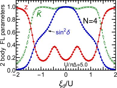
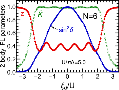
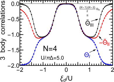
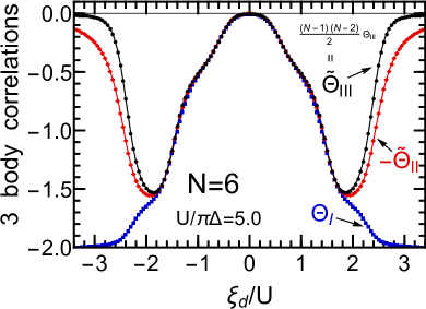
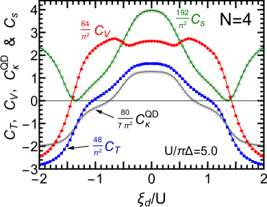
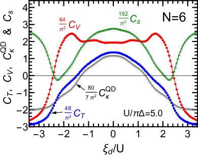
Figure 1: Fermi-liquid parameters for SU($N$) Anderson model are plotted vs $\xi_{d}\equiv\epsilon_{d}+(N-1)U/2$ for $U/(\pi\Delta)=5.0$, $N=4$ (left panels) and $N=6$ (right panels). Top panels: $\sin^{2}\delta$, renormalization factor $z$, and $\widetilde{K}\equiv(N-1)(R-1)$. Middle panels: $\Theta_{\mathrm{I}}$, $\,\,-\widetilde{\Theta}_{\mathrm{II}}\equiv-(N-1)\Theta_{\mathrm{II}}$, and $\,\,\widetilde{\Theta}_{\mathrm{III}}\equiv\frac{(N-1)(N-2)}{2}\Theta_{\mathrm{III}}$. Bottom panels: $\frac{48}{\pi^{2}}C_{T}$, $\frac{64}{\pi^{2}}C_{V}$, $\frac{80}{7\pi^{2}}C_{\kappa}^{\mathrm{QD}}$, and $\frac{192}{\pi^{2}}C_{S}$.

The top panels of Fig. 1 show the two-body correlations, relating to $\,\langle n_{d\sigma}\rangle$, $\chi_{\sigma\sigma}$, and $\chi_{\sigma\sigma^{\prime}}$. We see that $\sin^{2}\delta$, which determines $\mathcal{T}_{\sigma}(0)$ at $T=eV=0$, shows a flat Kondo ridge of the unitary limit $\delta\simeq\pi/2$ near the PH symmetric point $|\xi_{d}|\lesssim U/2$ where the occupation number is almost locked at $N_{d}\simeq N/2$. The other Kondo ridges also emerge at $\xi_{d}$ where $N_{d}$ approaches an integer: $\xi_{d}\simeq\pm U$ for $N=4$, and also $\xi_{d}\simeq\pm U,\pm 2U$ for $N=6$.

The renormalization factor $z$, which determines the energy scale $T^{*}=z\,\pi\Delta/(4\sin^{2}\delta)$, is also shown in the top panels. It is significantly suppressed over a wide range of gate voltages $|\xi_{d}|\lesssim\frac{N-1}{2}U$, and appears as a broad valley. This valley becomes shallow as $N$ increases, and vanishes in the large $N$ limit Oguri (2012). Inside the valley, $z$ has minimums at $\xi_{d}\simeq\frac{N-2M}{2}\,U$ for $M=1,2,\ldots,N-1$, where the occupation number approaches an integer $N_{d}=M$. At these minimums, the low-energy states can be described by the SU($N$) Kondo model in the strong-coupling limit $U\gg\Delta$. We find that $z$ is also suppressed at local maximums corresponding to the intermediate valence states, for both $N=4$ and $6$. In the top panels, the rescaled Wilson ratio $\widetilde{K}$ is also shown. It is almost saturated to the universal value $\widetilde{K}=1$ and its derivative becomes very small ${\partial\widetilde{K}}/{\partial\epsilon_{d}}\sim 0$ in the whole region of the broad valley $1\lesssim N_{d}\lesssim N-1$. It reveals the fact that not only the charge susceptibility $\chi_{c}\equiv-{\partial\langle n_{d\sigma}\rangle}/{\partial\epsilon_{d}}=\chi_{\sigma\sigma}(1-\widetilde{K})$ but its derivative ${\partial\chi_{c}}/{\partial\epsilon_{d}}$ is suppressed in this region.

The three-body correlation $\Theta_{\mathrm{I}}$ is plotted in the middle panels of Fig.  1, together with the other two rescaled ones: $\,-\widetilde{\Theta}_{\mathrm{II}}\equiv-(N-1)\Theta_{\mathrm{II}}$, and $\,\widetilde{\Theta}_{\mathrm{III}}\equiv\frac{(N-1)(N-2)}{2}\Theta_{\mathrm{III}}$. These $\Theta$’s also show plateau structures due to the Kondo effect at the values of $\xi_{d}$ corresponding to integer $N_{d}$, and almost vanish at $|\xi_{d}|\lesssim\frac{U}{2}$. We find that these three parameters $\Theta_{\mathrm{I}}$, $\,-\widetilde{\Theta}_{\mathrm{II}}$, and $\widetilde{\Theta}_{\mathrm{III}}$ approach each other very closely over a wide gate-voltage range $|\xi_{d}|\lesssim\frac{N-2}{2}\,U$, at which $1\lesssim N_{d}\lesssim N-1$. This indicates that contributions of the diagonal element $\chi_{\sigma\sigma\sigma}^{[3]}$ dominate the terms in the right-hand side of Eq. (4); i.e. $\chi_{\sigma\sigma\sigma}^{[3]}$ becomes much greater than $\frac{\partial\chi_{\sigma\sigma}}{\partial\epsilon_{d}}$ and $\frac{N-1}{2}\,\frac{\partial\chi_{\sigma\sigma^{\prime}}}{\partial\epsilon_{d}}$. It also reveals the fact that not only $\partial\chi_{c}/\partial\epsilon_{d}$ but also $\partial\chi_{s}/\partial\epsilon_{d}$, the derivative of the spin susceptibility $\chi_{s}\propto\chi_{\sigma\sigma}-\chi_{\sigma\sigma^{\prime}}$, becomes much smaller than $(T^{*})^{-2}$. Thus, for large $U$, the FL properties are characterized by three parameters $\,\delta$, $T^{*}$ and $\Theta_{\mathrm{I}}$ over the wide filling range $1\lesssim N_{d}\lesssim N-1$. Outside this region, the $\Theta$’s approach the noninteracting values: $\Theta_{\mathrm{I}}\to-2$, and the other two vanish as $|\xi_{d}|\to\infty$.

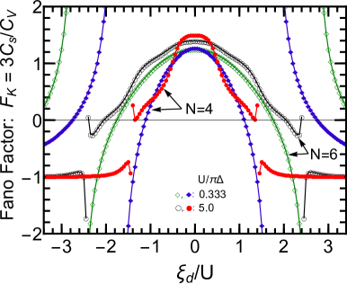
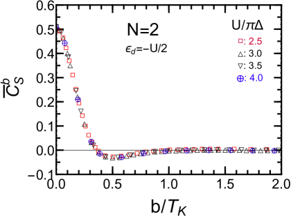
Figure 2: Nonlinear current-current correlations. Left panel: $F_{K}\equiv\frac{C_{S}}{C_{V}/3}$ vs $\xi_{d}/U$ for SU($N$) symmetric case for $N=4$ ($\bullet$, $\blacklozenge$) and $N=6$ ($\circ$,$\lozenge$), for $U/(\pi\Delta)=1/3$ (diamonds) and $U/(\pi\Delta)=5$ (circles). Right panel: $\overline{C}_{S}^{b}$ vs $b/T_{K}$ for $N=2$ at half filling $\epsilon_{d}=-U/2$, for $U/(\pi\Delta)=2.5,3.0,3.5,4.0$, with $b$ the magnetic field and $T_{K}$ the Kondo temperature at $b=0$.

Nonequilibrium FL fluctuations.— We show in the following how the transport coefficients evolve as $N_{d}$ varies continuously. The NRG results are also plotted in Fig. 1. The difference between the $C$’s near half filling $|\xi_{d}|\lesssim\frac{U}{2}$ is caused by the two-body contributions $W$’s as the $\Theta$’s almost vanish. In particular, the $T^{2}$ conductance $C_{T}$ is determined by $W_{T}$ over the wide filling range $1\lesssim N_{d}\lesssim N-1$ as the three-body contributions almost cancel out $\Theta_{\mathrm{I}}+(N-1)\,\Theta_{\mathrm{II}}\approx 0$, reflecting the suppression of $\partial\chi_{c}/\partial\epsilon_{d}$ and $\partial\chi_{s}/\partial\epsilon_{d}$ mentioned above. For the thermal conductivity, the three-body contributions become negative in this region, $\Theta_{\mathrm{I}}+\frac{5}{21}(N-1)\,\Theta_{\mathrm{II}}\approx-\frac{16}{21}\,\widetilde{\Theta}_{\mathrm{II}}$, but otherwise $C_{\kappa}^{\mathrm{QD}}$ shows a similar $\xi_{d}$ dependence to that of $C_{T}$. The three-body contributions on the $(eV)^{2}$ conductance $C_{V}$ are given by $\Theta_{V}\equiv\Theta_{\mathrm{I}}+3(N-1)\,\Theta_{\mathrm{II}}$, which takes a value $\Theta_{V}\approx 2\,\widetilde{\Theta}_{\mathrm{II}}$ in the same filling range. Thus, $C_{V}$ is significantly enhanced at $N_{d}\simeq 1$ and $N-1$ where $-\widetilde{\Theta}_{\mathrm{II}}$ shows a deep valley. It pushes the tail of the $C_{V}$ curve outside than that of the $C_{T}$ in the valence fluctuation region towards the empty or fully-occupied limit.

The $|eV|^{3}$ current noise also exhibits the Kondo plateau structures as shown in Fig. 1. For $C_{S}$, the three-body contributions enter through $\Theta_{V}$ with a sinusoidal factor: $-\Theta_{V}\cos 2\delta\approx\frac{\sin 4\delta}{2\pi}\,\frac{\chi_{\sigma\sigma\sigma}^{[3]}}{\chi_{\sigma\sigma}^{2}}$ over the range of $1\lesssim N_{d}\lesssim N-1$. In the valence fluctuation regions mentioned above, $C_{S}$ has a minimum caused by the higher-harmonic $\sin 4\delta$ and $\cos 4\delta$ contributions. We also find that $C_{S}$ approaches zero almost simultaneously with $C_{V}$ at $|\xi_{d}|\simeq 1.4U$ for $N=4$, and at $|\xi_{d}|\simeq 2.4U$ for $N=6$. This proximity of the zero points affects the behavior of an extended Fano factor $F_{K}$, defined as the ratio of order $(eV)^{3}$ current noise to the nonlinear current Mora et al. (2015, 2009); Note (2):

$$\!\!F_{K}\equiv\lim_{|eV|\to 0}\frac{S_{\mathrm{noise}}^{\mathrm{QD}}-\frac{2Ne^{2}|eV|}{h}\,\frac{\sin^{2}2\delta}{4}}{-2|e|\,\left(J-\frac{Ne^{2}|V|}{h}\,\sin^{2}\delta\right)}\,=\,\frac{C_{S}}{C_{V}/3}.$$ (7)

This formula for the SU($N$) Anderson model includes the result of Mora et al, obtained for $N=2$ at zero magnetic field Mora et al. (2015), as a special case. In the strong coupling limit at integer $N_{d}$, it also agrees with another noise formula of Mora et al for the SU($N$) Kondo model Mora et al. (2009).

The Fano factor for $N=4,6$ is plotted vs $\xi_{d}$ for two different values of $U$ in the left panel of Fig. 2. It reaches the local maximum $F_{K}\to(N-1+9\widetilde{K}^{2})/(N-1+5\widetilde{K}^{2})$ at $\xi_{d}=0$ Sakano et al. (2011), and has positive plateaus for large $U$ at integer $N_{d}$. In the limit of $|\xi_{d}|\to\infty$, the ratio becomes negative and takes the noninteracting value $F_{K}\to-1$. By definition, $F_{K}$ changes sign at the zero points of $C_{S}$. It also diverges at the zero point of $C_{V}$, where the nonlinear component of $J$ changes direction from backward to forward. Such a singularity already exists for $U=0$ at $|\xi_{d}|={\Delta}/{\sqrt{3}}$. For large $U$, $F_{K}$ diverges near $|\xi_{d}|\simeq\frac{N-1}{2}U$ in the valence fluctuation region towards the empty or fully-occupied limit. We can see that sign of the coefficient $C_{S}$ at the singular points becomes positive for large $U$, whereas it is negative for small $U$. Sign change occurs, for both $N=4$ and $6$, at a finite $U$ between the two examined cases $U/(\pi\Delta)=1/3$ and $5$. It is associated with the large enhancement of three-body contributions $\Theta_{V}$ occurring in the Kondo regime at $N_{d}\simeq 1$ and $N-1$ for $N>2$. In contrast, the NRG calculations examined so far indicate that sign is always negative in the SU(2) case for any $U\geq 0$ Mora et al. (2015); Note (2). The main difference is that in the SU(2) case the three-body correlations evolve in the valence fluctuation region where electron correlations become less important and the two-body contributions $W_{S}$ dominate $C_{S}$ near the singular point.

Magnetic-field dependence.— We next consider effects of a magnetic field $b$ that breaks the SU($N$) and TR symmetries: specifically at half filling for $N=2$, where $\epsilon_{d\uparrow}=-\frac{U}{2}-b$, $\epsilon_{d\downarrow}=-\frac{U}{2}+b$, and the electron filling is fixed at $\langle n_{d\uparrow}\rangle+\langle n_{d\downarrow}\rangle=1$. In this case, the transport coefficients can be described also by five FL parameters: magnetization $m_{d}\equiv\langle n_{d\uparrow}\rangle-\langle n_{d\downarrow}\rangle$, susceptibilities $\chi_{\uparrow\uparrow}$ $=\chi_{\downarrow\downarrow}$ and $\chi_{\uparrow\downarrow}=\chi_{\downarrow\uparrow}$, and three-body correlations $\chi_{\uparrow\uparrow\uparrow}^{[3]}=-\chi_{\downarrow\downarrow\downarrow}^{[3]}$ and $\chi_{\uparrow\downarrow\downarrow}^{[3]}=-\chi_{\uparrow\uparrow\downarrow}^{[3]}$. The nonlinear current for this case has previously been studied Oguri and Hewson (2018a, b); Filippone et al. (2018). However, behavior of its fluctuations has not been clarified so far.

Here, we examine the current noise at $T=0$ :

$$S_{\mathrm{noise}}^{\mathrm{QD}}\,=\,\frac{4e^{2}|eV|}{h}\left[\,\frac{\sin^{2}(\pi m_{d})}{4}\ +\ \overline{C}_{S}^{b}\left(\frac{eV}{T_{K}}\right)^{2}+\cdots\,\right].$$

Note that the second term is scaled by $T_{K}\equiv\left.T^{*}\right|_{b=0}$, the Kondo temperature defined at zero field. Thus, the coefficient $\overline{C}_{S}^{b}$ includes all effects of $b$, which enter through the FL parameters. In the right panel of Fig. 2, NRG results for $\overline{C}_{S}^{b}$ are plotted as a function of $b/T_{K}$ for several different values of $U$. We find that the nonlinear noise exhibits a universal behavior for $U/(\pi\Delta)\gtrsim 2.0$ in a similar way that the nonlinear current shows Oguri and Hewson (2018a, b). It decreases rapidly as $b$ increases for small fields, changes sign at $b\approx 0.36T_{K}$, takes a minimum at $b\approx 0.5T_{K}$, and then approaches zero at $b\gtrsim T_{K}$. We note that order $T^{3}$ thermal conductivity also exhibits the scaling behavior Note (2). These observations reflect the fact that the three-body fluctuations show the universal scaling behavior in the Kondo regime without the TR symmetry.

Conclusion.— Nonlinear transport through the SU($N$) Anderson impurity has been described in a unified way with five FL parameters. We have demonstrated how the FL state evolves as electron filling $N_{d}$ varies, using the NRG up to $N=6$. For strong interactions $U$, not only charge fluctuations but also the derivatives of charge and spin susceptibilities are suppressed over a wide filling range $1\lesssim N_{d}\lesssim N-1$. It reduces the number of variable FL parameters from five to three, and causes the Kondo plateau structures emerging for all the coefficients $C$’s. In particular, the three-body contributions on $C_{V}$ are significantly enhanced at $N_{d}\simeq 1$ and $N-1$ for $N>2$. It also affects the behavior of nonlinear Fano factor $F_{K}$ in the valence fluctuation region. We have also shown that the nonlinear current noise exhibits the universal magnetic-field scaling in the Kondo regime. The FL parameters can also be deduced from experiments and can be used to predict behaviors of unmeasured observables.

We would like to thank K. Kobayashi, T. Hata, M. Ferrier, R. Deblock, and A. C. Hewson for valuable discussions. This work was supported by JSPS KAKENHI Grand Numbers JP18J10205, JP18K03495, JP26220711, and JST CREST Grant No. JPMJCR1876.

Fermi liquid theory for nonlinear transport through a multilevel Anderson impurity (Supplemental Material)

I.  Derivation of the transport coefficients $\,C_{T}$, $C_{V}$ and $C_{\kappa}^{\mathrm{QD}}$

We describe here outline of the derivation of the coefficients $C$’s, listed in table 1 in the main text. The steady current $J$ through the quantum dots has been calculated using the formula given in Eq. (3) with the transmission probability, defined by

$$\mathcal{T}_{\sigma}(\omega)\,= \ \frac{-4\Gamma_{L}\Gamma_{R}}{\Gamma_{L}+\Gamma_{R}}\ \mathrm{Im}\,G_{\sigma}^{r}(\omega)\,,\qquad\qquad G_{\sigma}^{r}(\omega)\,=\,\frac{1}{\omega-\epsilon_{d\sigma}+i\Delta\,-\Sigma_{\sigma}^{r}(\omega)}\;.$$ (8)

We have also calculated the thermal conductivity $\kappa_{\mathrm{QD}}$, which can be expressed in the following form at $eV=0$,

$$\kappa_{\mathrm{QD}}=\frac{1}{2\pi\hbar T}\left[\sum_{\sigma}\mathcal{L}_{2,\sigma}^{\mathrm{QD}}-\frac{\left(\sum_{\sigma}\mathcal{L}_{1,\sigma}^{\mathrm{QD}}\right)^{2}}{\sum_{\sigma}\mathcal{L}_{0,\sigma}^{\mathrm{QD}}}\right]\,,\qquad\qquad\quad\mathcal{L}_{n,\sigma}^{\mathrm{QD}}\,\equiv\,\int_{-\infty}^{\infty}d\omega\,\omega^{n}\ \mathcal{T}_{\sigma}(\omega)\,\left(-\frac{\partial f(\omega)}{\partial\omega}\right).$$ (9)

The coefficients for the charge and heat currents, $C_{T}$, $C_{V}$, and $C_{\kappa}^{\mathrm{QD}}$, can be deduced form the low-energy expansion of the retarded self-energy $\Sigma_{\sigma}^{r}(\omega)$ obtained up to terms of order $\omega^{2}$, $T^{2}$, and $(eV)^{2}$. We note that, in order to determine also the thermopower of quantum dots $\mathcal{S}_{\mathrm{TP}}^{\mathrm{QD}}$ up to next leading order, additional terms of order $\omega^{3}$ and $\omega\,T^{2}$ of the self-energy are necessary. This is because the leading term of $\mathcal{S}_{\mathrm{TP}}^{\mathrm{QD}}$ already includes the derivative $\rho_{d\sigma}^{\prime}\equiv\frac{\partial\rho_{d\sigma}(\omega)}{\partial\omega}\big{|}_{\omega=0}$ which describes a variation from the ground state:

$$\mathcal{S}_{\mathrm{TP}}^{\mathrm{QD}}\,\equiv\,\frac{-1}{|e|T}\frac{\sum_{\sigma}\mathcal{L}_{1,\sigma}^{\mathrm{QD}}}{\sum_{\sigma}\mathcal{L}_{0,\sigma}^{\mathrm{QD}}}\ =\ -\,\frac{\pi^{2}}{3|e|}\frac{\sum_{\sigma}\rho_{d\sigma}^{\prime}}{\sum_{\sigma}\rho_{d\sigma}}\ T\,+\,O(T^{3})\,,\qquad\qquad\qquad\rho_{d\sigma}^{\prime}\,=\,\frac{\chi_{\sigma\sigma}\,\sin 2\delta_{\sigma}}{\Delta}\,.$$ (10)

The expansion coefficients of $\Sigma_{\sigma}^{r}(\omega)$ can be expressed in terms of the linear and nonlinear susceptibilities,

$$\mathrm{Im}\,\Sigma_{\sigma}^{r}(\omega)\ = \ -\,\frac{\pi(N-1)}{2}\,\frac{\chi_{\sigma\sigma^{\prime}}^{2}}{\rho_{d\sigma}}\,\left[\,\omega^{2}+\frac{3}{4}\,(eV)^{2}+(\pi T)^{2}\,\right]+\cdots\,,\qquad\qquad\quad(\sigma^{\prime}\neq\sigma)\;,$$ (11)

$$\epsilon_{d}+\mathrm{Re}\,\Sigma_{\sigma}^{r}(\omega)\,= \ \ \Delta\,\cot\delta\,+\left(1-\widetilde{\chi}_{\sigma\sigma}\right)\omega+\,\frac{1}{2}\frac{\partial\widetilde{\chi}_{\sigma\sigma}}{\partial\epsilon_{d\sigma}}\,\omega^{2}\,+\,\frac{N-1}{6}\,\frac{\chi_{\sigma\sigma^{\prime}\sigma^{\prime}}^{[3]}}{\rho_{d\sigma}}\left[\,\frac{3}{4}(eV)^{2}+\left(\pi T\right)^{2}\,\right]+\cdots\;,$$ (12)

for $\Gamma_{L}=\Gamma_{R}=\Delta/2$ and $\mu_{L}=-\mu_{R}=eV/2$ in the SU($N$) symmetric case. Note that $\widetilde{\chi}_{\sigma\sigma^{\prime\prime}}\equiv\delta_{\sigma\sigma^{\prime\prime}}+\left.\frac{\partial\Sigma_{\sigma}^{r}(0)}{\partial\epsilon_{d\sigma^{\prime\prime}}}\right|_{T=eV=0}$, $\,\chi_{\sigma\sigma^{\prime\prime}}=\rho_{d\sigma}\widetilde{\chi}_{\sigma\sigma^{\prime\prime}}$, and $\rho_{d\sigma}=\sin^{2}\delta/(\pi\Delta)$ for $\sigma=1,2,3,\ldots,N$. These results are obtained by extending further the latest version of Fermi-liquid description [A. Oguri and A. C. Hewson, Phys. Rev. B 97, 035435] to the multilevel cases $N>2$. At $T=eV=0$, the self-energy satisfies the Ward identity of the following form, which yields the Fermi-liquid relations between the expansion coefficients,

$$\left(\delta_{\sigma\sigma^{\prime}}\,\frac{\partial}{\partial\omega}\ +\ \frac{\partial}{\partial\epsilon_{d\sigma^{\prime}}}\right)\Sigma_{\sigma}^{--}(\omega)\ =\ -\,\Gamma_{\sigma\sigma^{\prime};\sigma^{\prime}\sigma}^{--;--}(\omega,0;0,\omega)\,\rho_{d\sigma^{\prime}}\;.$$ (13)

Here, $\Sigma_{\sigma}^{--}(\omega)=\mathrm{Re}\,\Sigma_{\sigma}^{r}(\omega)+i\,\mathrm{sgn}(\omega)\,\mathrm{Im}\,\Sigma_{\sigma}^{r}(\omega)$, and $\Gamma_{\sigma\sigma^{\prime};\sigma^{\prime}\sigma}^{--;--}(\omega,\omega^{\prime};\omega^{\prime},\omega)$ is the causal vertex function at $T=eV=0$. It has been determined up to linear order terms with respect to $\omega$ and $\omega^{\prime}$,

$$\Gamma_{\sigma\sigma;\sigma\sigma}^{--;--}(\omega,\omega^{\prime};\omega^{\prime},\omega)\rho_{d\sigma}^{2}\,= \ i\pi\sum_{\sigma^{\prime}(\neq\sigma)}\chi_{\sigma\sigma^{\prime}}^{2}\bigl{|}\omega-\omega^{\prime}\bigr{|}\ +\ \cdots\;,\qquad\qquad\qquad\qquad(\sigma^{\prime}\neq\sigma)\;,$$ (14)

$$\Gamma_{\sigma\sigma^{\prime};\sigma^{\prime}\sigma}^{--;--}(\omega,\omega^{\prime};\omega^{\prime},\omega)\,\rho_{d\sigma}\rho_{d\sigma^{\prime}}\,= \ -\chi_{\sigma\sigma^{\prime}}+\rho_{d\sigma}\frac{\partial\widetilde{\chi}_{\sigma\sigma^{\prime}}}{\partial\epsilon_{d\sigma}}\,\omega+\rho_{d\sigma^{\prime}}\frac{\partial\widetilde{\chi}_{\sigma^{\prime}\sigma}}{\partial\epsilon_{d\sigma^{\prime}}}\,\omega^{\prime}+i\pi\,\chi_{\sigma\sigma^{\prime}}^{2}\,\Bigl{(}\,\bigl{|}\omega-\omega^{\prime}\bigr{|}-\,\bigl{|}\omega+\omega^{\prime}\bigr{|}\,\Bigr{)}+\cdots\;.$$ (15)

The Ward identity itself follows from the current conservation between the dot and leads:

$$\frac{\partial}{\partial t}\,(e\,n_{d\sigma}^{\phantom{0}})+\widehat{J}_{R,\sigma}-\widehat{J}_{L,\sigma}=0,\qquad\quad\widehat{J}_{L,\sigma}\equiv i\,ev_{L}\left(\psi^{\dagger}_{L\sigma}d_{\sigma}-d^{\dagger}_{\sigma}\psi_{L\sigma}\right),\qquad\widehat{J}_{R,\sigma}\equiv-i\,ev_{R}\left(\psi^{\dagger}_{R\sigma}d_{\sigma}-d^{\dagger}_{\sigma}\psi_{R\sigma}\right)\;.$$ (16)

 

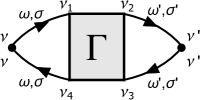
Figure 3: The Feynman diagrams for the correlation function $\int_{-\infty}^{\infty}\!dt\,\mathcal{K}_{\sigma^{\prime}\sigma}^{\nu^{\prime}\nu}(t,0)$. The solid lines denote the Keldysh Green’s functions $G_{\sigma}^{\nu^{\prime}\nu}(\omega)$. The shaded region in the diagram on the right represents the Keldysh vertex function $\Gamma_{\sigma\sigma^{\prime};\sigma^{\prime}\sigma}^{\nu_{1}\nu_{2};\nu_{3}\nu_{4}}(\omega,\omega^{\prime};\omega^{\prime}\omega)$. The superscripts $\nu$, $\nu^{\prime}$ and $\nu_{i}$ ($i=1,2,3,4$) specify the branches of Kedysh time-loop contour. We are using the notation in which $\nu=-$ and $+$ represent the forward and return paths, respectively.

II.  Fermi-liquid corrections for nonlinear current noise $\,S_{\mathrm{noise}}^{\mathrm{QD}}$

In contrast to the average current $J$ and thermal conductivity $\kappa_{\mathrm{QD}}$, the current noise depends also on the two-quasiparticle collisions which correspond to the vertex corrections for the current-current correlation function $\mathcal{K}_{\sigma^{\prime}\sigma}^{\nu^{\prime}\nu}$:

$$S_{\mathrm{noise}}^{\mathrm{QD}}\,= \ \int_{-\infty}^{\infty}\!\!dt\ \sum_{\sigma\sigma^{\prime}}i\Bigl{[}\,\mathcal{K}_{\sigma^{\prime}\sigma}^{+-}(t,0)+\mathcal{K}_{\sigma^{\prime}\sigma}^{-+}(t,0)\,\Bigr{]}\;,\qquad\qquad\delta\widehat{J}_{\sigma}(t)\equiv\widehat{J}_{\sigma}(t)-\langle\widehat{J}_{\sigma}(t)\rangle_{V}\,,$$ (17)

$$\mathcal{K}_{\sigma^{\prime}\sigma}^{+-}(t,0)\,\equiv \ -i\,\bigl{\langle}\delta\widehat{J}_{\sigma^{\prime}}(t)\,\delta\widehat{J}_{\sigma}(0)\bigr{\rangle}_{V}\,,\qquad\qquad\mathcal{K}_{\sigma^{\prime}\sigma}^{-+}(t,0)\,\equiv\,-i\,\bigl{\langle}\delta\widehat{J}_{\sigma}(0)\,\delta\widehat{J}_{\sigma^{\prime}}(t)\bigr{\rangle}_{V}\;\rule{0.0pt}{17.07182pt}\,.$$ (18)

Here, $\widehat{J}_{\sigma}\equiv(\Gamma_{L}\widehat{J}_{R,\sigma}+\Gamma_{R}\widehat{J}_{L,\sigma})/(\Gamma_{L}+\Gamma_{R})$ is a symmetrized current operator. In this work, we have expanded $S_{\mathrm{noise}}^{\mathrm{QD}}$ up to terms of order $(eV)^{3}$, using the diagrammatic representation illustrated in Fig. 3. To this end, all the components of Keldysh Green’s function $G_{\sigma}^{\nu^{\prime}\nu}(\omega)$ have been deduced up to order $\omega^{2}$ and $(eV)^{2}$, and the Keldysh vertex function $\Gamma_{\sigma\sigma^{\prime};\sigma^{\prime}\sigma}^{\nu_{1}\nu_{2};\nu_{3}\nu_{4}}(\omega,\omega^{\prime};\omega^{\prime}\omega)$ have been calculated up to linear order in $\omega$, $\omega^{\prime}$ and $eV$. We have checked that the result satisfies the nonequilibrium Ward identity [A. Oguri, Y. Tetatani, and S. Sakano, unpublished],

$$\left(\delta_{\sigma\sigma^{\prime}}\,\frac{\partial}{\partial\omega}+\frac{\partial}{\partial\epsilon_{d\sigma^{\prime}}}\right)\Sigma_{\sigma}^{\nu_{4}\nu_{1}}(\omega)\,=\,-\int_{-\infty}^{\infty}\!\frac{d\omega^{\prime}}{2\pi}\,\sum_{\nu_{2}\nu_{3}}\,\Gamma_{\sigma\sigma^{\prime};\sigma^{\prime}\sigma}^{\nu_{1}\nu_{2};\nu_{3}\nu_{4}}(\omega,\omega^{\prime};\omega^{\prime},\omega)\ 2\Delta\,G_{\sigma^{\prime}}^{r}(\omega^{\prime})\,G_{\sigma^{\prime}}^{a}(\omega^{\prime})\,\left(-\frac{\partial f_{\mathrm{eff}}(\omega^{\prime})}{\partial\omega^{\prime}}\right)\,.$$ (19)

Here, $f_{\mathrm{eff}}(\omega)=\bigl{\{}\Gamma_{L}\,f_{L}(\omega)+\Gamma_{R}\,f_{R}(\omega)\bigr{\}}/(\Gamma_{L}+\Gamma_{R})$, and $\Sigma_{\sigma}^{\nu_{4}\nu_{1}}(\omega)$ is the Keldysh self-energy. The expansion coefficient for order $(eV)^{3}$ current noise is given in table 1. It can be separated into two parts $C_{S}=C_{S}^{\mathrm{qp}}+C_{S}^{\mathrm{coll}}$, as mentioned in the main text. Here, $C_{S}^{\mathrm{qp}}$ and $C_{S}^{\mathrm{coll}}$ represent respectively the contributions of the bubble diagram and that of the vertex corrections shown in Fig. 3.

The nonlinear Fano factor, $F_{K}=\frac{C_{S}}{C_{V}/3}$, can be expressed in the following form for the SU($N$) Anderson impurity at arbitrary electron fillings,

$$F_{K}\,=\,\frac{\cos 4\delta\,+\Bigl{[}\,4+5\cos 4\delta+\frac{3}{2}\bigl{(}1-\cos 4\delta\bigr{)}\,(N-2)\,\Bigr{]}\,\displaystyle\frac{\widetilde{K}^{2}}{N-1}\,-\,\cos 2\delta\,\Bigl{[}\,\Theta_{\mathrm{I}}+3\,(N-1)\Theta_{\mathrm{II}}\,\Bigr{]}}{-\left[1+5\,\displaystyle\frac{\widetilde{K}^{2}}{N-1}\right]\cos 2\delta\,+\,\Theta_{\mathrm{I}}+3\,(N-1)\Theta_{\mathrm{II}}}\;.$$ (20)

For $N=2$, it reproduces the previous result, obtained by Mora et al [Eq. (11) of Phys. Rev. B 92, 075120 (2015)]: their notation and our one correspond to each other such that $\alpha_{\sigma}^{(1)}/\pi=\chi_{\sigma\sigma}$, $\phi_{\sigma\sigma^{\prime}}^{(1)}/\pi=-\chi_{\sigma\sigma^{\prime}}$, $\alpha_{\sigma}^{(2)}/\pi=-\frac{1}{2}\,\chi_{\sigma\sigma\sigma}^{[3]}$, and $\phi_{\sigma\sigma^{\prime}}^{(2)}/\pi=2\,\chi_{\sigma\sigma^{\prime}\sigma^{\prime}}^{[3]}$ for $\sigma^{\prime}\neq\sigma$. In Fig. 4, we have also plotted $F_{K}$ and other Fermi-liquid parameters for the SU(2) symmetric case as functions of $\epsilon_{d}$ for comparisons with those for $N=4$ and $6$ shown in the main text.

Equation (20) also reproduces the previous result in the particle-hole symmetric case, at which $\delta=\pi/2$ and the three-body contributions vanish $\Theta_{\mathrm{I}}=\Theta_{\mathrm{II}}=0$ [Sakano et al Phys. Rev. B 83 , 075440 (2011)] :

$$F_{K}\,\xrightarrow{\,\epsilon_{d}\to-(N-1)U/2\,}\,\frac{1+\frac{9\widetilde{K}^{2}}{N-1}}{1+\frac{5\widetilde{K}^{2}}{N-1}}\,\xrightarrow{\,U\to\infty\,}\,\frac{1+\frac{9}{N-1}}{1+\frac{5}{N-1}}\,.$$ (21)

In the strong coupling limit $U\to\infty$, the occupation number $N_{d}\equiv\sum_{\sigma}\langle n_{d\sigma}\rangle$ becomes integer $M=1,\,2,\,\ldots,N-1$ at $\epsilon_{d}=-(M-1/2)U$ and the phase shift is locked at $\delta=\pi M/N$. The charge and spin susceptibilities satisfy the stationary conditions in this case, and thus Eq. (20) can be rewritten as

$$\!\!\!\!\!\!\!\!\!\!\!\!\!\!\!\!\!\!\!\!F_{K}\ \to \ \frac{1+\sin^{2}\left(\frac{2\pi M}{N}\right)\,+\frac{9-13\sin^{2}\left(\frac{2\pi M}{N}\right)}{N-1}\ +\ 2\,\Theta_{\mathrm{I}}\,\cos\left(\frac{2\pi M}{N}\right)}{-\left[\,1+\frac{5}{N-1}\,\right]\cos\left(\frac{2\pi M}{N}\right)-2\,\Theta_{\mathrm{I}}}\;.$$ (22)

This expression is consistent with the corresponding noise formula for the SU($N$) Kondo model, obtained by Mora et al [Eq. (51) of Phys. Rev. B 80, 155322 (2009), after inserting some parenthesis for correcting minor typos].

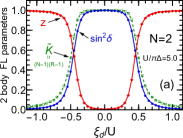
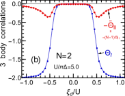
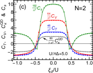
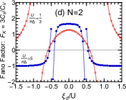
Figure 4: Fermi-liquid parameters for the SU(2) symmetric case are plotted vs $\xi_{d}\equiv\epsilon_{d}+U/2$ for $U/(\pi\Delta)=5.0$. (a): $\sin^{2}\delta$, renormalization factor $z$, and $\widetilde{K}\equiv(N-1)(R-1)$. (b): thee-body correlatins $\Theta_{\mathrm{I}}$, and $\,\,-\widetilde{\Theta}_{\mathrm{II}}\equiv-(N-1)\Theta_{\mathrm{II}}$. (c): $\frac{48}{\pi^{2}}C_{T}$, $\frac{64}{\pi^{2}}C_{V}$, $\frac{192}{\pi^{2}}C_{S}$, and $\frac{80}{7\pi^{2}}C_{\kappa}^{\mathrm{QD}}$. (d): nonlinear Fano factor $F_{K}=\frac{C_{S}}{C_{V}/3}$ is plotted also for $U/(\pi\Delta)=1/3,\,5$.

III.  NRG calculations

NRG calculations for the SU($N$) Anderson model for $N=2,4,6$ have been carried out, dividing $N$ channels into $N/2$ pairs and exploiting the SU(2) spin and U(1) charge symmetries for each of the pairs, i.e.  using $\prod_{k=1}^{\frac{N}{2}}\left\{\mbox{SU(2)}\otimes\mbox{U(1)}\right\}_{k}$ symmetries. The discretization parameter $\Lambda$ and the number of retained low-lying excited states $N_{\mathrm{trunc}}$ are chosen such that $(\Lambda,N_{\mathrm{trunc}})=(2,4000)$ for $N=2$, $\,(6,10000)$ for $N=4$, and $\,(20,30000)$ for $N=6$. We have also exploited methods of Stadler’s et al [Phys. Rev. B 93, 235101 (2017)] for $N=6$. The truncation is performed at each step after adding states from each pair of the channels, using Olivera’s $\mathcal{Z}$-trick [Phys. Rev. B 49, 11986 (1994)] and choosing different $\mathcal{Z}$ values for different pairs: $\mathcal{Z}_{i}=1/2+i/N$ for the $i$-th pair ($i=1,2,\ldots,N/2$).

Table 2: The coefficients $C$’s at finite magnetic fields $b$ for $N=2$ at half filling $\epsilon_{d}=-\frac{U}{2}$.

See also, A. Oguri and A. C. Hewson, Phys. Rev. B 98, 079905 (E). $C_{S}^{b}\ =\,\frac{\pi^{2}}{192}\left[\,W_{S}^{b}+\left(\Theta_{\mathrm{I}}^{b}+3\Theta_{\mathrm{II}}^{b}\right)\,\cos(\pi m_{d})\,\right]$      $W_{S}^{b}\,\equiv\,\cos(2\pi m_{d})+\bigl{[}\,4+5\cos(2\pi m_{d})\,\bigr{]}(R-1)^{2}$ $C_{V}^{b}\,=\,\frac{\pi^{2}}{64}\,\bigl{[}\,W_{V}^{b}\,+\,\Theta_{\mathrm{I}}^{b}+3\,\Theta_{\mathrm{II}}^{b}\,\bigr{]}$       $W_{V}^{b}\,\equiv\,\left[\,1+5\left(R-1\right)^{2}\,\right]\cos(\pi m_{d})$ $C_{T}^{b}\,=\,\frac{\pi^{2}}{48}\,\bigl{[}\,W_{T}^{b}\,+\,\Theta_{\mathrm{I}}^{b}+\Theta_{\mathrm{II}}^{b}\,\bigr{]}\quad$      $W_{T}^{b}\ \equiv\,\left[\,1+2\left(R-1\right)^{2}\,\right]\cos(\pi m_{d})$ $C_{\kappa,b}^{\mathrm{QD}}=\,\frac{7\pi^{2}}{80}\,\bigl{[}\,W_{\kappa,b}^{\mathrm{QD}}\,+\,\Theta_{\mathrm{I}}^{b}+\frac{5}{21}\Theta_{\mathrm{II}}^{b}\,\bigr{]}$      $W_{\kappa,b}^{\mathrm{QD}}\,\equiv\,\left[\,1+\frac{6}{7}\left(R-1\right)^{2}\,\right]\cos\left(\pi m_{d}\right)$

IV.  Magnetic-field dependence of current noise for $N=2$

We describe here supplemental information about the nonlinear current noise at finite magnetic field $b$, specifically for $N=2$ at half filling, where the impurity level is given by $\epsilon_{d\sigma}\equiv-\frac{U}{2}-\mathrm{sgn}(\sigma)\,b$ with $\mathrm{sgn}(\uparrow)=+1$ and $\mathrm{sgn}(\downarrow)=-1$. In this case, the phase shift takes the form $\delta_{\sigma}=\pi\{1+\mathrm{sgn}(\sigma)\,m_{d}\}/2$ with $m_{d}\equiv\langle n_{d\uparrow}\rangle-\langle n_{d\downarrow}\rangle$, and the other correlation functions have symmetry properties: $\,\chi_{\uparrow\uparrow}=\chi_{\downarrow\downarrow}$, $\,\chi_{\uparrow\downarrow}=\chi_{\downarrow\uparrow}$, $\,\chi_{\uparrow\downarrow\downarrow}^{[3]}=-\chi_{\uparrow\uparrow\downarrow}^{[3]}$, and $\,\chi_{\downarrow\downarrow\downarrow}^{[3]}=-\chi_{\uparrow\uparrow\uparrow}^{[3]}$. Thus, the transport coefficients up to the next leading order can be described by five parameters, for instance, $m_{d}$, $T^{*}=1/(4\chi_{\uparrow\uparrow})$, $R=1-\chi_{\uparrow\downarrow}/\chi_{\uparrow\uparrow}$ and the following 3-body correlation functions,

$$\!\!\!\Theta_{\mathrm{I}}^{b}\equiv-\frac{\sin(\pi m_{d})}{2\pi}\,\frac{\chi_{\uparrow\uparrow\uparrow}^{[3]}}{\chi_{\uparrow\uparrow}^{2}},\quad\ \Theta_{\mathrm{II}}^{b}\equiv-\frac{\sin(\pi m_{d})}{2\pi}\frac{\chi_{\uparrow\downarrow\downarrow}^{[3]}}{\chi_{\uparrow\uparrow}^{2}}.$$ (23)

The low-energy expansion of the current noise $S_{\mathrm{noise}}^{\mathrm{QD}}$, conductance $dJ/dV$, and thermal conductivity $\kappa_{\mathrm{QD}}$ for this case can be written in the following form, with the coefficients $C$’s listed in table 2,

$$\!\!S_{\mathrm{noise}}^{\mathrm{QD}}=2\,\frac{2e^{2}}{h}|eV|\!\left[\frac{\sin^{2}(\pi m_{d})}{4}+C_{S}^{b}\left(\frac{eV}{T^{*}}\right)^{2}\!\!+\cdots\right]\!,\!$$ (24)

$$\!\!\frac{dJ}{dV}=\frac{2e^{2}}{h}\!\left[\cos^{2}\left(\frac{\pi m_{d}}{2}\right)-C_{T}^{b}\left(\frac{\pi T}{T^{*}}\right)^{2}\!-C_{V}^{b}\left(\frac{eV}{T^{*}}\right)^{2}\!\!+\cdots\right]\!,$$

$$\!\!\kappa_{\mathrm{QD}}=\frac{2\pi^{2}T}{3h}\left[\cos^{2}\left(\frac{\pi m_{d}}{2}\right)-C_{\kappa,b}^{\mathrm{QD}}\left(\frac{\pi T}{T^{*}}\right)^{2}\!+\cdots\right].$$

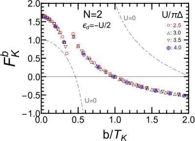
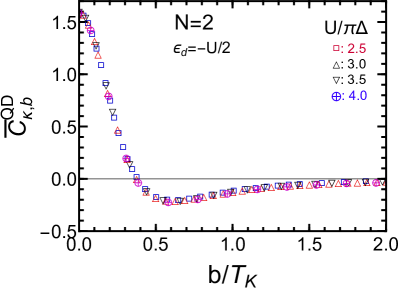
Figure 5: $F_{K}^{b}=\frac{\overline{C}_{S}^{b}}{\overline{C}_{V}^{b}/3}$ and $\overline{C}_{\kappa,b}^{\mathrm{QD}}\equiv(T_{K}/T^{*})^{2}C_{\kappa,b}^{\mathrm{QD}}$ for $N=2$ are plotted vs $b/T_{K}$ at half filling for $U/(\pi\Delta)=2.5,3.0,3.5,4.0$: $T_{K}$ varies with $U$, and $T_{K}\xrightarrow{U\to 0\,}\pi\Delta/4$.

In order to see the magnetic field dependences in the Kondo regime, it is preferable to rescale the next leading $(eV)^{2}$ and $T^{2}$ contributions by the Kondo temperature defined at zero field $T_{K}=\lim_{b\to 0}T^{*}$. This is because all effects of $b$ are absorbed into the coefficients redefined such that $\,\overline{C}_{V}^{b}\equiv(T_{K}/T^{*})^{2}\,C_{V}^{b}$, $\,\overline{C}_{S}^{b}\equiv(T_{K}/T^{*})^{2}\,C_{S}^{b}$, and $\overline{C}_{\kappa,b}^{\mathrm{QD}}\equiv(T_{K}/T^{*})^{2}\,C_{\kappa,b}^{\mathrm{QD}}$. We have presented the NRG results for the nonlinear current noise $\overline{C}_{S}^{b}$ in the main text; $\overline{C}_{V}^{b}$ was examined previously [A. Oguri and A. C. Hewson, Phys. Rev. Lett. 120, 126802 (2018)]. In Fig. 5, $F_{K}^{b}\equiv\frac{C_{S}^{b}}{C_{V}^{b}/3}$ and $\overline{C}_{\kappa,b}^{\mathrm{QD}}$ are plotted as functions of $b/T_{K}$ for several different values of $U$. The nonlinear Fano factor $F_{K}^{b}$ shows the Kondo scaling behavior for strong interactions $U/(\pi\Delta)\gtrsim 2.0$. The universal curve of $F_{K}^{b}$ deviates significantly from the curve for $U=0$ keeping its qualitative characteristics unchanged. We also find that the thermal conductivity $\overline{C}_{\kappa,b}^{\mathrm{QD}}$ exhibits the universal scaling behavior.

References

Hewson (1993)A. C. Hewson, The Kondo Problem to
Heavy Fermions (Cambridge University Press, 1993).
Delattre et al. (2009)T. Delattre, C. Feuillet-Palma, L. G. Herrmann, P. Morfin,
J.-M. Berroir, G. FShu ve, B. PlaXun ais, D. C. Glattli, M.-S. Choi, C. Mora, and T. Kontos, Nature
Physics 5, 208 (2009).
Yamauchi et al. (2011)Y. Yamauchi, K. Sekiguchi,
K. Chida, T. Arakawa, S. Nakamura, K. Kobayashi, T. Ono, T. Fujii, and R. Sakano, Phys. Rev. Lett. 106, 176601 (2011).
Ferrier et al. (2016)M. Ferrier, T. Arakawa,
T. Hata, R. Fujiwara, R. Delagrange, R. Weil, R. Deblock, R. Sakano, A. Oguri, and K. Kobayashi, Nat. Phys. 12, 230 (2016).
Laird et al. (2015)E. A. Laird, F. Kuemmeth,
G. A. Steele, K. Grove-Rasmussen, J. Nygård, K. Flensberg, and L. P. Kouwenhoven, Rev.
Mod. Phys. 87, 703
(2015).