Abstract

A broad and widely used class of stationary, linear, additive time series models can have statistical properties which many authors have asserted imply that the underlying process must be non-linear, non-stationary, multiplicative, or inconsistent with shot noise. This result is demonstrated with exact and numerical evaluation of the model flux distribution function and dependence of flux standard deviation on mean flux (here and in the literature called the rms-flux relation). These models can: (1) exhibit normal, log-normal or other flux distributions; (2) show linear or slightly non-linear rms-mean flux dependencies; as well as (3) match arbitrary second order statistics of the time series data. Accordingly the above assertions cannot be made on the basis of statistical time series analysis alone. Also discussed are ambiguities in the meaning of terms relevant to this study – linear, stationary and multiplicative – and functions that can transform observed fluxes to a normal distribution as well or better than the logarithm.

1 Introduction

A widespread goal in the study of stochastic variation of astronomical systems is to explore underlying physical processes, which are unfortunately not directly observable. In a seminal paper Press (1978) coined the evocative term flickering (now often called $1/f$ noise or colored noise), and commented that explanation of physical and astrophysical processes variable on all timescales had been exceedingly difficult. There has since been considerable progress, for example through improved data analysis methods (e.g. Vaughan, 2013) and through study of explicitly non-linear, chaotic dynamical models (e.g. Scargle, Donoho, Crutchfield et al., 1992; Mineshige, Ouchi and Nishimori, 1994; Aschwanden, 2011).

However, the inner workings of astrophysical systems remain largely mysterious. This fact is probably not due to a data shortage, in view of the great advances in observational capabilities in modern astronomy. Elucidating complex, dynamic, three-dimensional astrophysical systems – with uncertain physical processes and parameters – from one-dimensional time series data is intrinsically difficult. But an important added factor is the tortuous path from time series data to inferred dynamical properties, strewn with misunderstandings about the nature of their connections.

It is the purpose of this note to clarify some of these problematic issues in analyzing distributions of observed fluxes, and dependencies between flux and flux variance. A new derivation of properties of a broad class of linear, stationary, and additive processes demonstrates that they can possess linear and near-linear variance-mean flux relations and arbitrary flux distributions, including the range from normal to log-normal and beyond. Therefore such statistical properties of light curves should not be taken to indicate the presence of non-linearity, non-stationarity, or multiplicativity, or to disallow the presence of shot-noise characteristics, as frequently asserted.

A partial summary of previous work is followed by clarification of how the relevant terms linear, stationary, additive, and their opposites, are used here. Subsequent sections briefly define standard autoregressive/moving average (ARMA) random process models, and then analyze the rms vs. mean flux relation and flux-distribution properties of the models. Extensions to incorporate some forms of nonstationarity, short- and long- term memory, and fractional Brownian motion, beyond the scope here, are worth further study – e.g. the autoregressive fractionally integrated moving average (ARFIMA) models discussed in Granger and Joyeux (1980).

2 Previous Work

Denis et al. (1994) were apparently the first to report “source noise flux” linearly increasing with “source total flux,” using x-ray observations of Nova Persei. The influential paper Uttley and McHardy (2001) elaborated this idea, importantly broadening the class of sources that demonstrate a linearly increasing dependence of root-mean-square variability on mean flux. Detailed X-ray light curves of Cyg X-1 and SAX J1808.4-3658 showed a remarkably tight linear relation, and three Seyfert galaxies showed similar dependence, albeit with crude flux resolution.

Since this initial work, the linear “rms vs flux” relation has been extended by various authors to many sources and source classes, leading to the attribution of near ubiquity to this relation. A key paper (Uttley et al., 2005) reported a detailed analysis in the context of X-ray binaries and active galaxies. Vaughan and Uttley (2008) discuss tests for non-linearity, non-Gaussianity, and time asymmetry using statistics beyond second order. Giebels and Degrange (2009) commented on the approximately log-normal flux distribution and a relatively scattered rms-mean flux relation in BL Lacertae. Heil, Vaughan and Uttley (2012) found the rms-flux relation present in several black hole binaries, with systematic dependence of the slope and intercept on hardness state. Scaringi et al. (2012) found linear rms-flux relations in Kepler data for the white dwarf MV Lyrae. Dobrotka and Ness (2015) looked for a rms-flux relation in Kepler data for V1504 Cyg, finding it in quiescent time intervals and, in modified form, in outbursts. Kushwaha, Sinha, Misra, Kingh, and de Gouveia Dal Pino (2017) and Shah et al. (2018) report log-normal flux distributions in Fermi Gamma-Ray Space Telescope (FGST) blazar data. Alston (2019) studied non-stationarity and other time series properties using simulations.

Some work has attempted to link relevant observations with theoretical models. The study of accretion-disk fluctuations by Lyubarskii (1997), while not directly addressing the issues discussed here, has influenced some work that does. Hogg and Reynolds (2016) studied propagating fluctuations in MHD models of turbulent disk accretion, in connection with log-normalcy and linear rms-mean flux relations. Phillipson, Boyd and Smale (2018) compared topological features of return maps of X-ray light curves of the binary 4U1705-44 and those of a system exhibiting non-linear chaotic behavior. Sinha, Khatoon, Mistra at al. (2018) addressed the possibility that linear Gaussian variations of particle acceleration and escape times can produce non-Gaussian flux distributions, including log-normal ones. Dobrotka, Negoro and Mineshige (2019) studied a model for fast variability. Bhatta and Dhital (2019) find log-normal flux distributions and linear rms-mean flux relations in Fermi gamma-ray data for 20 blazars, discussing possible contact with models with propagating relativistic shocks.

Recent work includes identification of non-linear rms-mean flux (that is, with some curvature), in sources and wavelengths where neither rms-mean flux relations nor log-normality are present, and a simple model for linear rms-mean flux relations. Edelson, Mushotzky, Vaughan et al. (2013) displayed non-linear rms-flux relations in Kepler data for the BL Lac galaxy W2R1926+42. Smith et al. (2018), in a study of 21 AGN Kepler optical light curves, found neither log-normal flux distributions nor rms-flux relations; Smith adds that there is no evidence for an rms-flux relation in any analysis of the best-studied Kepler AGN Zw229-15 in particular (private communication). Alston, Fabian, Buisson et al. (2019) find a non-linear rms-flux dependence rms $\propto$ flux^2/3 in x-ray time series for the Seyfert galaxy IRAS 13224-3809. Of course it is hard to know to what extent there have been studies where relevant negative results were not published. Koen (2016) has proposed a model in which the rms-mean flux relation is due to simple scaling effects, spurring a response by Uttley, McHardy and Vaughan (2017) asserting that without modification Koen’s model does not yield linear rms-flux relations on a wide range of time scales or log-normal flux distributions.

These and other authors have advanced a variety of often conflicting conjectures about underlying physical processes, based on statistical characteristics of light curves. Below evidence against such conjectures is provided by the result that the relevant attributes are produced by simple, general, and naturally motivated statistical models – without reference to specific physical mechanisms, nor any element of non-linearity nor of non-stationarity nor of multiplicativity. In some cases more recent authors seem to have misunderstood or ignored caveats in the foundational work in, e.g. (Uttley et al., 2005, Appendix D) and Uttley, McHardy and Vaughan (2017). Any criticism implied by the discussion below is aimed at the tangled web of interactions between various ideas, and not at specific authors.

3 Time Series Descriptors

It is hoped that the reader will excuse the didactic nature of this discussion, in view of confusions in terminology describing statistical properties of time series permeating the literature. In view of the importance of clarity in scientific communication, ambiguous short-hand terminology – especially in scientific publications, but even in informal settings such as white-board discussions – are appropriate only if all participants understand the same meanings.

In regimes of non-linear growth of structures, cosmologists call the absolute square of the (linear) Fourier transform of the mass density field the non-linear power spectrum. Meant as a convenient shorthand, this usage can be misleading in several ways. It uses a term defined in one domain (gravitational clustering of matter) in a qualitatively different domain (second-order statistics of spatial data), i.e. applying a physics-based descriptor to something non-physical. And it suggests that unambiguous signatures of nonlinear physics can appear directly in the power spectrum.

This section addresses terms describing properties of mathematical models or physical processes. Importing these concepts to time series data analysis, albeit from these well-defined settings, can be fraught with vagueness, ambiguity and confusion. When there is more than one applicable meaning, short-hand terminology is confusingly ambiguous without clear definition of the sense intended. Special circumstances and assumptions necessary in the mathematical or physical contexts can be forgotten, ignored, or insufficiently understood as applied to data. The imported concept may refer to statistics that cannot be directly estimated from the data alone.

The following sub-sections elaborate common threads in three yin-yang pairs: linear/non-linear, stationary/non-stationary, and additive/multiplicative, in each case attempting to describe how physical or mathematical properties can give one the impression that the term applies to time series data. Similar considerations apply to other dualities, such as causal/acausal, minimum/maximum delay, time-reversal invariant/non-invariant, and analytic/non-analytic (Pascual-Granado, Garrido and Suárez, 2013, 2015), but are not discussed here.

3.1 Is Linearity Meaningful for Time Series?

The concepts of linearity and non-linearity, well defined in mathematics and some physics contexts, have seeped into areas of astrophysics where they are not well defined. In the context of random flickering in astronomical light curves, linearity is a property of processes (applying to mathematical or physical systems) but not to time series data. To describe light curves as linear or non-linear, without extension or generalized definition, is a category error – ascribing to something a property that by definition cannot apply to it. These facts are recognized in some quarters, but terms like “linear data” and “non-linear time series” appear frequently in the literature, often without qualification or explanation. Approaches range from taking these terms to be so unambiguous that the plain meaning rule applies and no definition is required, to thoughtful consideration of clear definitions. Unfortunately the latter is much rarer than the former. Accordingly it is useful to consider three contexts, as follows:

Mathematics: Here the concept is simple: function $F(x)$ is linear in its argument if

$$F(x+y) = F(x)+F(y)$$ (1)

$$F(ax) = aF(x)$$ (2)

for arbitrary $x$, $y$ and $a$. Usages in other contexts – e.g. linear term characterizing the first order part of a Taylor series expansion, or a term in an equation proportional to the independent variable – derive from this relation.

Physics: This mathematical concept can be extended to only those physical systems with a clearly identified and quantitative input/output property – corresponding to $F$ mapping an input into an output. A textbook example is a spring: an applied force (input) produces a stretch of the spring (output). In Physics 1 we learn Hooke’s law: within limits the displacement (output $F$) is linear in the applied force (input $x$) but becomes non-linear with larger force if there are corrections to Equation (2). This concept rarely applies to complicated systems as a whole, and is undefined unless it is possible to identify an idealized subsystem with the input-output property. Even then it applies only to that subsystem, which may or may not be a primary determinant of an observable such as the time evolution of flux. In theoretical physics one encounters much the same mathematical concepts described above.

Astrophysics: Even a complex astronomical object typically has a well defined output: its emitted flux. If there is a “mechanism” turning some “input” into all or part of this flux, both of these are largely unknown (or hypothetical in the case of a physical model). Indeed, the goal of the analysis is to identify and elucidate these. Most often there are many mechanisms, or sub-processes, interacting with each other in various ways. Some of these are perhaps describable as input-output systems, others not. It seems unlikely that unambiguous linearity/non-linearity signatures due to a single “central engine” will appear commonly in light curves for such systems. Nevertheless, let us explore some possible ways to attribute meaning to such properties in time series data.

Perhaps the simplest idea springs from fitting simple parametric time-domain models directly to light curves, as simple as linear trends. Comparison of descriptions of the data using linear and non-linear regression can obviously be made to yield definitions of linearity or non-linearity. While this concept is only indirectly related to dynamics, it may be what some analysts have in mind.

Another approach is to compare descriptions using dynamics-motivated linear and non-linear models of the time evolution of the observable. The entire book by Priestley (1988) is devoted to this viewpoint. Time series data better described by models of the latter class could be said to be non-linear. Brockwell and Davis (1987) frame linearity in terms of equivalence of optimal and linear prediction. An example of a linear model is the autoregressive/moving average process described below. The Volterra process (Priestley, 1988; Uttley et al., 2005) – essentially a Taylor series expansion generalizing the autoregressive formalism with a potentially infinite series of explicitly nonlinear terms – is an example of a non-linear model. There is a fundamental problem with applying this approach to stationary processes: The Wold Theorem guarantees the existence of a linear model exactly representing any stationary process, even if it is in some sense putatively non-linear. That is, within the context of stationarity, these models “fit” the data precisely as well as Volterra models – or any other non-linear model for that matter.

Another obvious problem of this enormous generalization is nicely described by Granger and Anderson (1978): “At first sight, there may seem to be an overpowering richness of possibilities once the linear constraint on models is removed.” These authors slightly ameliorate this difficulty by adding “ … but if certain sensible restrictions are placed on the models, very many of the possibilities can be removed.” (One such restriction is the admittedly subjective constraint that models have intuitive appeal. Another is not “exploding off to infinity at an exponential rate.” A third is a subtle concept called invertibility.) Comparison of linear against non-linear models will be dependent on the classes of models of each form considered, potentially leading to much uncertainty of the results. Theoretical constraints or other considerations – such as parsimony, an important model simplicity principle – may reduce the size and complexity of the model space.

Yet another problem is the need for a quantitative goodness-of-fit measure of some sort to compare models. Simple mean error measures are not necessarily applicable: since autoregressive models reproduce the data exactly (see Section 4), model quality is assessed via properties of the random driving process (called the innovation; see below). Comparison of models using different quantitative measures is obviously fraught with difficulties.

A somewhat different approach is to attempt to measure non-linearity in the form of a metric associated with non-linear (“chaotic”) dynamics (Tong, 1990; Theiler, Lindday and Rubin, 1993; Buchler and Kandrup, 1997; Sprott, 2003). In addition to the fact that such analyses typically rely on very long sequences of high signal-to-noise data (e.g., to ensure many near-returns to the same state), rare in astronomy, there are fundamental estimation problems as described by Osborne and Provenzale (1989); Ruelle (1990); Eckmann and Ruelle (1992). Theiler, Lindday and Rubin (1993) discuss other practical difficulties and caveats with the use of surrogate data in this context. Some recent developments (Phillipson, Boyd and Smale, 2018, e.g.) in this area show progress at overcoming such limitations.

An approach, often implicit rather than clearly defined, is to interpret large amplitude flares as signatures of non-linearity. Of course “small amplitude = linear; large amplitude = non-linear” can, with care, be turned into an unambiguous criterion. However its connection to the mathematical and physical concepts described above is illusory without caveats or assumptions about the underlying physics. (E.g. “I believe the underlying mechanism has an input-output feature that accords with such-and-such amplitude-based criterion.) That this approach is not generally useful is demonstrated by the fact that many linear models can yield arbitrarily large amplitude flares; for example there is no a priori limit to the dynamic range of the model guaranteed, for any stationary process, even if putatively non-linear, by the Wold Theorem.

In summary, the concept of non-linearity does not transport well to time series in general, and astronomical light curves in particular. Several possible ways to implant linearity concepts into astronomical time series analysis lack the necessary carefully crafted definitions and physical assumptions, raising the suspicion that the term is employed without any meaning or idea (as is but too frequent).

3.2 Is Stationarity Meaningful for Time Series?

As with linearity, attempts to define stationarity run afoul of pragmatic difficulties when applied to time series data. Standard definitions invoke time invariance of statistical quantities. For example constancy of the mean and variance is termed weak stationarity; constancy of all possible probability distributions is strong stationarity. Many other definitions of stationarity are possible, based on invariance of various statistical properties. The concept of asymptotic stationarity (Parzen, 1962) accounts for a system decaying away from its initial state, approaching one of these forms of stationarity in the limit (see Thorne and Blandford, 2017, Sec. 6.2 for a physics setting). In non-linear dynamics an important related concept is transient chaos (Young and Scargle, 1996): non-linear pseudo random behavior evolving asymptotically to a steady state.

In principle these theoretical concepts require infinite stretches of data to rigorously test for time invariance. Therefore importing the concepts into a realistic data analysis context requires care. A useful concept of stationarity must specify how independence is to be judged, the degree of approximation required, and the operative time scale or range. Furthermore, data apparently stationary on one time scale can easily appear non-stationary on another scale, e.g. over a longer interval – and vice versa. In short, the appearance of data within the finite window presented by the observations can be misrepresentative of the actual variability, both random and systematic. Even pulsar rotation, one of the best examples of approximate astronomical stationarity, suffers from non-stationarity on long time scales through spindown; in addition short time scale “glitches” may or may not be approximately stationary,

This issue is related to one raised nearly a century ago in the classic paper (Yule, 1926) dealing with the fact “that we sometimes obtain between quantities varying with the time … quite high correlations to which we cannot attach any physical significance whatsoever, although under the ordinary test the correlation would be held to be certainly ‘significant’.” Yule’s cross-correlation problem is in a different context, but his finite-sampling and “cosmic variance” issues are much the same for stationarity. A common confusion arises from random variability on two different time-scales, where it is tempting to leap to the view that the slower variations are nonstationary when judged against the faster ones.

The unavoidable conclusion that stationarity is “in the eye of the beholder” carries with it certain ambiguities and subjectivities. Any assessment of this property is dependent on (a) the above mentioned qualitative and quantitative description of method and relevant time scales, (b) any theoretical or other astrophysical considerations incorporated in the judgement, and (c) any preprocessing of the data, such as removal of trends or intense flares. Any of these issues can dramatically affect conclusions about stationarity. The point is that the corresponding choices need to be clearly stated, not that any one or the other is right or wrong. Furthermore, analysis of the data separately under both hypotheses (stationary and non-stationary) may be productive. In the end, stationarity is fraught with nearly as many problematic issues as linearity.

Note that in Section 4 we make use of the consequences of strict mathematical stationarity, and therefore our results must be used with appropriate caution, with an eye toward possible effects of non-stationarity. In this regard autoregressive-integrated-moving average (ARIMA) models (Scargle, 1981b, e.g.), constructed to represent some forms of non-stationarity, may have some application.

3.3 Is Multiplicativity Meaningful for Time Series?

The term multiplicative (e.g. Uttley et al., 2005) is similarly transplanted – with some of the same issues discussed above – from mathematics to physics to time series. In physics the concept posits a separation of the system into subsystems, each of which contributes a component to the total flux. Such a compound process is termed additive or multiplicative depending on whether the resulting output is the sum or product of that due to the components. Applicability of this concept depends on whether separation into largely independent subsystems is valid, and on the correctness of the prescription for combining their flux contributions. Justification for this idea is sometimes sought from its success in other areas of research and from log-normal distributions (log of product = sum of logs = normalcy as opposed to sum of normals = normal, both via the central limit theorem). Here the term additive refers mostly to the representation of time series as the sum of random events, as will now be detailed.

4 The Random Process Models

A well-known, powerful and flexible model expresses stationary random processes as the output of a linear system driven by a random input. This model is known in different fields under various names, including: autoregressive, moving average, autoregressive-moving average, Ornstein-Uhlenbeck, Brownian motion, damped random walk, and shot noise. Only the discrete forms of continuous models are of relevance here. These stationary, linear, and additive models are essentially equivalent to each other, differing mainly in their formal definition and physical interpretation. The autoregressive (AR) and moving average (MA) models discussed in this section are surrogates for members of this class.

The Wold Decomposition Theorem (Wold, 1938) states that any stationary process can be represented in the form of the so-called moving average (not the same as running mean)

$$X(n)=\sum_{k}c_{k}R(n-k)+D(n)\ \ ;$$ (3)

$X(n)$ in the current setting is the flux at discrete time $n$ and $R(n)$ is an uncorrelated random process (called the innovation). Stationarity is the only necessary condition; any other notion, such as linearity, is irrelevant. The set of constants $\{c_{k}\}$, called the moving average coefficients, has two technical properties relating to the model flare shape: causality and minimum-delay. This remarkably explicit representation of the random and non-random aspects of an arbitrary stationary process, and their separation into two additive terms, are among many notable features of the Wold Decomposition (Scargle, 1981a, b; Brockwell and Davis, 1987). The component $D$ is a deterministic process, largely ignored here. In practice it is often a constant that can be removed, e.g. with the novel background estimation procedure described by Meyer, Scargle and Blandford (2019), or a slowly varying function, removable with a detrending procedure.

It is important to realize that Equation (3) is a theoretical relationship, asserting the formal equivalence of the random process on either side of the equal sign. Furthermore, there is a family of representations of a given stationary process equivalent to each other in this same sense. For example, entirely equivalent to the moving average form in Equation (3) is this autoregressive representation of the same process, with the same innovation:

$$X(n)=\sum_{k}a_{k}X(n-k)+R(n)\ \ .$$ (4)

Memory of previous behavior, the Markov property, is expressed by the autoregressive coefficients $\{a_{k}\}$. The term ${a}_{k}X(n-k)$ is the contribution to $X(n)$ of self-memory of the process $k$ steps prior to the time $n$. These forms – denoted AR($K$) or MA($K$), where $K$ is the number of terms included – are simply different ways to represent the same random process. Formally a finite AR(K) process is equivalent to MA($\infty$), and a finite MA(K) to AR($\infty$); of course in practice finite approximate versions are used. These two representations have different astrophysical interpretations, as we will now see.

It is quite natural to picture the moving average as modeling the observed flux $X(n)$ at time $n$ as the superposition of randomly occurring flares (also called pulses, events, shots, filters, etc., depending on context), for which the term shot-noise is often used. The flare shape is determined by the coefficients {$c_{k}$}. The flare amplitude at time $n$ is $R(n)$. See (Scargle, 1981a, b) for discussion of the role of independently distributed innovations, corresponding, e.g., to the assumption that the light curve is generated by physically separated subsystems not communicating with each other, whose outputs are therefore statistically independent. (If, on the other hand, $R$ is normally distributed the above model is a Gauss-Markov process, of no interest here for reasons outlined below.)

Figure (1) depicts three simulations of Eq. (3) differing only in the distribution of the innovation. For the sparsest case (the bottom curve) the events are relatively isolated from each other. For the middle curve the innovation is less sparse, so there is considerable overlap between events. The top curve approaches the Gaussian limit where the true flare shape cannot be determined by any algorithm, because the high degree of overlap hides all information beyond second order statistics.

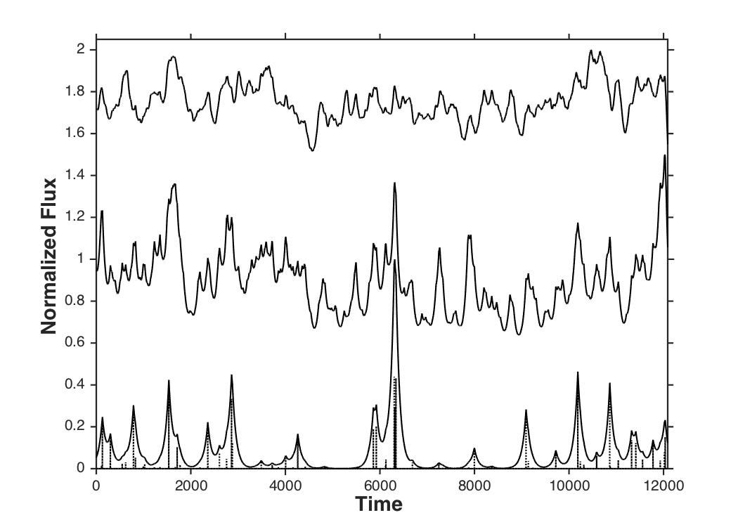
Figure 1: Simulated moving average light curves: Flare shape $C\sim$e${}^{-|t-t_{0}|/81.3}$, a symmetric two-sided exponential; innovations $R=U^{\alpha}$; $U$ uniformly distributed random numbers; $\alpha$ = 10 (top), 100 (middle), and for 1000 (bottom) U^α is also shown with dotted lines. By favoring large values and suppressing small ones, increasing $\alpha$ yields increasingly sparse innovations $U^{\alpha}$.

The autoregressive version of the Wold Representation, Equation (4) has the form of a linear system driven by a random input. While less visual, this interpretation can in principle be tied to a physical picture of an underlying dynamical process, with short- or long-term memory depending on the number of terms included. However one should keep in mind that the two models are equivalent, interchangeable representations. With a slightly different notation than adopted here, the AR and MA coefficients are convolutional inverses of each other. The innovation can be determined by convolving the time series data with an estimate of the AR coefficients. Then the modeled data, defined by convolving this innovation with the MA coeffecients, exactly reproduce the light curve. For more details see (Scargle, 1981b) or statistics textbooks (Priestley, 1988; Brockwell and Davis, 1987).

A few more comments on the significance of these models are in order. In both MA and AR formulations the innovation encodes the amplitudes of flare-like events. Its statistical distribution, not known a priori, is a key goal of data analysis. For astronomical light curves positive-definite innovations are relevant, because fluxes are non-negative. Gaussian innovations have the problem of negative values, as well the fact that the degeneracy among mixed-delay and mixed-causality models cannot be resolved for a Gaussian process by any algorithm (Scargle, 1981a, b). Crucially, then, astronomical time series data need to be modeled with positive definite, non-Gaussian innovations.

The Ornstein-Uhlenbeck process (OU), of importance in mathematical physics and increasingly invoked in astrophysics (Kelly et al., 2009; Kelly, Sobolewska, and Siemiginowska, 2011; Takata, Mukuto and Mizumoto, 2018; Kelly et al., 2014) is a continuous version of Equation (4) with only the $k=1$ term. It is usually defined as the solution of stochastic differential equations such as the Langevin equation, the Fokker-Planck equation, or a continuous version of AR(1) known as the Vasicek model in econometrics. The terms Brownian motion, damped random walk, and Lévy process are also used for essentially the same model. See Kelly et al. (2009) for application to quasar light curves and Kelly, Sobolewska, and Siemiginowska (2011) for further details. What is in common to all of these formalisms are the same properties described above: superposition of randomly occurring events (explicit in MA) and memory of the past (explicit in AR).

5 The RMS-Mean Flux Relation

The vaunted rms-mean flux relation explores possible dependence of flux variability on the flux itself. It is based on straightforward computation of the mean and standard deviation within subintervals of the total observation span. Free choices include the manner of correcting for observational noise (discussed below), the length and possible overlap of the subintervals, the binning employed in smoothing scatter plots, and possible data selection in the time or frequency domain. While Uttley, McHardy and Vaughan (2017) provide complete detail and Python code, some others do not give enough information for one to reproduce the results.

The frequently observed rms-mean flux behavior as described in Section 2 could derive from a universal physical process (e.g. turbulent accretion or jet dynamics), or from generic statistical properties of light-curves (e.g. stationarity or additivity). Evidence favoring the latter is next provided by demonstrating that AR and MA models, which are not based on specific physical processes, adequately reproduce the observed relations.

First note that observed fluxes based on photon counts have a built-in linear dependence of flux variance on mean flux (and hence a square-root dependence for the standard deviation) directly through photon counting fluctuations. Figure 2 demonstrates this fact by comparing a synthetic random light curve against a sampled version representing the additional variance due to photon count fluctuations. Such sampling is neither additive nor multiplicative, rather the result of applying an operator to the light curve to simulate observations that obey the Poisson distribution with mean photon rate equal to the source flux at each moment of time. As seen in the bottom right-hand panel these samples show the expected square-root rms dependence, shown as a line, easily mistakable for a linear relation over much of its extent.

This effect is probably not directly responsible for most of the reported rms-flux relationships. Uttley, McHardy and Vaughan (2017) provide a link to python code, which includes a correction subtracting the “… expected contribution of the observational error to the total variance … to give the intrinsic variance … ” Implementing this correction here, by taking such surrogate observational errors to be Poisson fluctuations, largely removes the dependence shown in the lower-right-hand panel of Figure 2. Nonetheless it is reasonable that imperfect estimation of, or accounting for, this photon counting contribution to the variance might affect the derived relation. It appears that some studies may have not carefully distinguished between observational and source-intrinsic variance in making this correction, or possibly not made the correction at all.

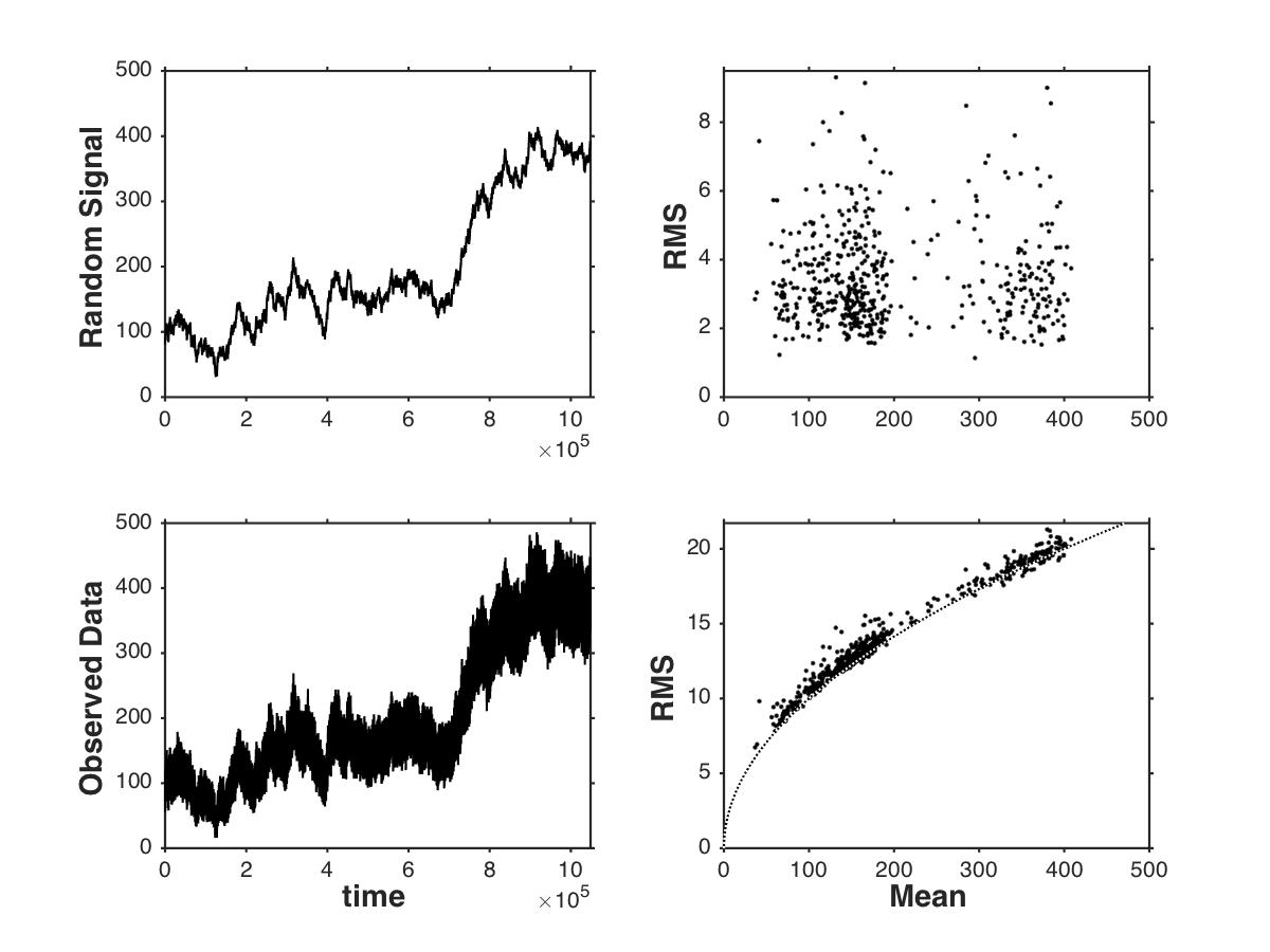
Figure 2: A simulated random walk time series. Upper-Left: cumulative sum of slightly biased normally distributed variables, renormalized. Lower-Left: The same data processed by applying the Poisson operator. Right Panels: scatter plots of root-mean-square flux vs. mean flux, derived from the corresponding data on the left-hand side. The solid line in the bottom-right panel is the theoretical square-root relation for the Poisson distribution. This figure demonstrates the effects of photon counting fluctuations, but for the most part these are accounted for in the data processing.

The relevant quantities are the mean and standard deviation of the flux, averaged over finite subintervals of the time series. Evaluating in this sense the expectation $E$ of the equation for the second order autoregressive model AR(2), i.e.

$$X(n)=aX(n-1)+bX(n-2)+R(n)\ ,$$ (5)

yields a linear relation between the flux and innovation means:

$$E(X)={1\over 1-a-b}E(R)\ .$$ (6)

The same relation follows from the moving average representation – cf. Eq. (14) below – yielding the intuitively expected result that the proportionality constant ${1\over 1-a-b}=\sum c_{k}$, the total area of the flare shape. To estimate the variance we need to find the mean of

$$X^{2}(n)=a^{2}X^{2}(n-1)+b^{2}X^{2}(n-2)+R^{2}(n)\\ +2abX(n-1)X(n-2)+2aX(n-1)R(n)+2bX(n-2)R(n)$$ (7)

Since previous values of $X$ are independent of the current value of the innovation, we have

$$E(X^{2})=a^{2}E(X^{2})+b^{2}E(X^{2})+E(R^{2})+2ab\ \rho(1)+2(a+b)E(X)E(R)\ ,$$ (8)

yielding

$$E(X^{2})={E(R^{2})+2ab\ \rho(1)+2(a+b)(1-a-b)E^{2}(X)\over(1-a^{2}-b^{2})}\ .$$ (9)

The variance $E(X^{2})-E^{2}(X)$ is thus

$$\sigma_{X}^{2}=\alpha E^{2}(X)+\beta\ ,$$ (10)

where

$$\alpha={2(a+b)(1-a-b)\over(1-a^{2}-b^{2})}$$ (11)

$$\beta={2a^{2}b\ \rho(0)\over(1-a^{2}-b^{2})(1-b)}+E(R^{2}){1\over 1-a^{2}-b^{2}}-E^{2}(R){1\over(1-a-b)^{2}}\ ,$$ (12)

using the Yule-Walker solution $\rho(1)=a\rho(0)/(1-b)$ (Priestley, 1988). For AR(1) simply set $b=0$:

$$\alpha={2a\over(1+a)};\hskip 36.135pt\beta=E(R^{2}){1\over 1-a^{2}}-E^{2}(R){1\over(1-a)^{2}}\ ,$$ (13)

Similar formulas can be obtained for the moving average representation. The expectation value of Eq. (3) gives

$$E(X)=E(R)\sum_{k}c_{k}\ ,$$ (14)

stating that the average output is the product of the area of the flare profile $C=\{c_{k}\}$, and the mean innovation. A further consequence of Eq. (3) is

$$E(X^{2})=\sum_{j}\sum_{k}c_{j}c_{k}E[R(n-j)R(n-k)]\ \ ,$$ (15)

giving, for the sum of the diagonal and off-diagonal terms, respectively:

$$E(X^{2})=E(R^{2})\sum_{j}c^{2}_{j}+E^{2}(R)\sum_{j\neq k}c_{j}c_{k}\ ,$$ (16)

yielding

$$\sigma^{2}_{X}=E(R^{2})\sum_{j}c^{2}_{j}+E^{2}(R)\sum_{j\neq k}c_{j}c_{k}-E^{2}(R)\sum_{j}\sum_{k}c_{j}c_{k}\ ,$$ (17)

or

$$\sigma^{2}_{X}=\sigma^{2}_{R}\sum_{j}c^{2}_{j}\ .$$ (18)

This tidy formula seems very different from Eq. (10) but is, in fact, equivalent to it. For the two relevant autoregressive models, this can be seen with a little algebra, e.g. using for AR(1) the sum $\sum_{j}c^{2}_{j}={1\over 1-a^{2}}$. While the two simplified expressions for variance as a function of the model parameters and innovation, are suggestive of a linear RMS-mean relation – Equation (10) if $\beta$ is small, and Equation (18) if $\sqrt{\sigma^{2}_{R}\sum_{j}c^{2}_{j}}\sim E(X)$ – the actual dependence on mean flux is implicit, not explicit.

If the distribution of $R$ is known, we can evaluate $\sqrt{\sigma^{2}_{R}}$. In the case of a power law distribution of the form

$$F(R)=F_{0}\ R^{\alpha}\ \ \mbox{for}\ \ 0\leq R\leq R_{0}\hskip 7.22743pt(0\ \ \mbox{otherwise})$$ (19)

it is straightforward to find the normalization factor

$$F_{0}=(\alpha+1)R_{0}^{-(\alpha+1)}$$ (20)

and the first and second moments

$$E(R)=F_{0}R_{0}^{\alpha+2}(\alpha+2)^{-1}\ ;\ \ \ \ E(R^{2})=F_{0}R_{0}^{\alpha+3}(\alpha+3)^{-1}\ ,$$ (21)

and with a bit of algebra

$$\sigma^{2}_{R}=(\alpha+1)(\alpha+2)^{-2}(\alpha+3)^{-1}R_{0}^{2}$$ (22)

Using Equation (14) to put this relation in a more easily interpretable form, we find

$$\sigma^{2}_{X}=(\alpha+1)^{-1}(\alpha+3)^{-1}{\sum c_{k}^{2}\over(\sum_{k}c_{k})^{2}}\ E^{2}(X)\ ,$$ (23)

corresponding to a linear rms-mean flux relation.

Turn now to numerical simulations. Figure 3 shows plots of $\sigma_{X}$ vs. E$(X)$ for the sample AR(1) process defined in the caption. The data used to make the figure are large sets of pairs of values, means and standard deviations, evaluated over non-overlapping sub-intervals. To avoid over-plotting that would confuse a simple scatter plot, this figure shows grey-scale representations of point density. In addition, for comparison with most published figures, points (show as circles) and error bars averaged over flux bins are displayed. The three panels cover a range of two orders of magnitude in sub-interval length. The dashed lines are fits to points generated by evaluating the square root of Equation (10) at the corresponding values of the abscissa.

For this particular model the figure demonstrates linear or slightly curved dependence of rms on mean flux. A small study of other model orders, parameters and innovations suggests that this result is characteristic of the class of autoregressive/moving average models, with the shape of the relation being determined by the distribution of the innovation as suggested by Equation (18). Importantly the non-linear rms-flux relations discussed by Alston, Fabian, Buisson et al. (2019) and Alston (2019) are curved in the same sense as in the first two panels of Figure 3. Some published scatter plots seem consistent with either linear or quadratic forms, within statistical uncertainties.

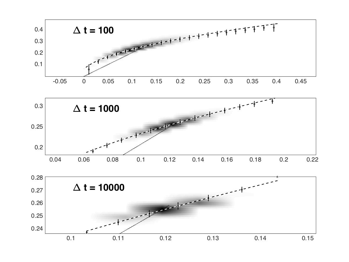
Figure 3: Grey scale plots of the density of points in the rms (standard deviation) vs. mean flux plane, for simulated AR(1) light curve: $a=0.5$, $R$ distributed as $U(4)$, i.e. uniform random numbers on $(0,1)$ raised to the power $4$, and truncated below 0.75. The total number of points generated is $N=2^{30}=1,073,741,825$. (No simulated observational errors were applied to these data.) Three different sizes of the time interval over which the averages were computed are indicated at the top-left of each panel; the corresponding number of points entering the density is $N$ divided by this number. The dashed lines are least-squares fits to Eq. (10) evaluated at these mean flux values. The dotted lines originate at (0,0) to indicate that the quasi-linear relations do not intersect the origin. The points and error bars are means and standard deviations averaged over a set of evenly spaced intervals.

By the way, the textbook power spectrum of the AR(2) process is

$$P(f)={\sigma_{X}^{2}\over 1+a^{2}+b^{2}+2a(1-b)\mbox{cos}(2\pi f)-2b\mbox{cos}(4\pi f)}\ \ .$$ (24)

The wide range of shapes yielded by this formula, samples of which are depicted in Figure 4, is perhaps not widely appreciated.

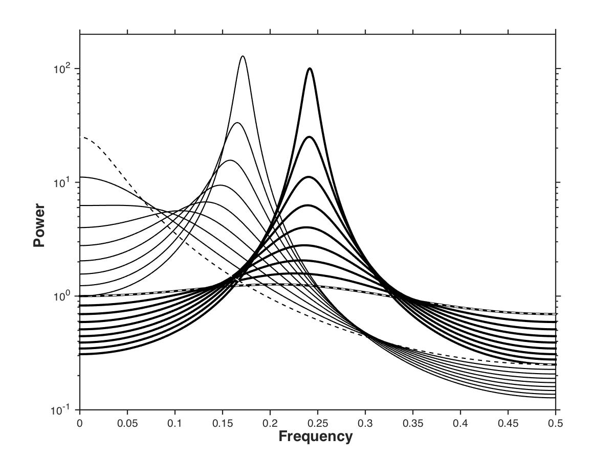
Figure 4: Logarithms of AR(2) power spectra from Equation (24); $a$ = -.1 (thick lines) and $a$ = -.9 (thin lines). In both cases $b$ ranges from -0.1 to -0.9 in steps of 0.1, with $b=-0.1$ a dashed line.

Section 3.5.3 of (Priestley, 1988) details the more intricate formula for the autocorrelation function. It is noteworthy that time series generated by this elementary model can display both random and quasi-periodic (Priestley uses the term pseudo-periodic) behavior, as suggested by Figure 4.

6 Flux Distributions

Wide interest in the distribution of measured flux values largely focuses on the binary choice between normal and log-normal (Crow and Shimizu, 1988). That this may be a false choice can be seen from the following computation of the exact distribution for an arbitrary autoregressive process.

A straightforward evaluation of the distribution $P_{X}(X)$ of $X$, in terms of the distribution $P_{R}(R)$ of the innovation $R$, starts from the moving average representation in Eq. (3). This equation holds for causal ($k>=0$), acausal ($k<=0$) and mixed representations ($k$ unconstrained). We invoke two text-book results: (1) The distribution of the sum of two random variables is the convolution of their distributions. (2) The distribution of a constant $C$ times a random variable $R$ is $P_{CR}(CR)={1\over C}P_{R}({R\over C})$. With these facts Equation (3) yields:

$$P_{X}(X)=\prod_{k}F_{c_{k}R}(c_{k}R)=\prod_{k}{1\over c_{k}}F_{R}({R\over c_{k}})\ ,$$ (25)

with $\prod$ denoting the convolution operation.

This formula is exact for an arbitrary moving average process. Figure 5 depicts these distributions for the special case of a first order autoregressive process with coefficient $a$. A monotonically decreasing power-law was chosen for the innovation distribution $P(R)$. For small values of $a$ – almost no memory of previous values – this output process is a nearly unaltered version of the input innovation, so the distribution is close to that of the innovation itself (shown as a thick dotted line). As $a$ increases the distribution broadens, for a while maintaining the high-end tail lending the appearance of log-normalcy. However, as $a$ approaches $1$, corresponding to a very strong memory, the distribution approaches a symmetric normal form; this is completely understandable through the central limit theorem and the fact that as $a\rightarrow 1$ many random variables are added together via equation (3). Of course this distribution must have zero weight for negative fluxes and cannot be exactly Gaussian.

In summary: the shape of the flux distribution for this linear process depends on two things: the distribution of the innovation and the value of the decay constant $a$. With a toy but not unrealistic power law distribution of input flare amplitudes (the innovation), distributions resembling normal or log-normal ones can be reproduced. Assertions that non-linear or “multiplicative” dynamical processes necessarily underly astrophysical systems based on log-normalcy are thus disproved.

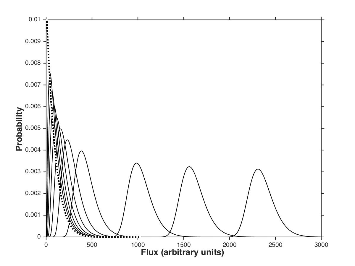
Figure 5: Flux distributions from AR(1) proceesses. The innovation is a power law distribution – $U^{10}$ in the notation in Scargle (1981b), i.e. a uniform distribution raised to the $10$th power – but reversed so that the probability decreases with increasing flux amplitude, and is plotted as a dotted line. The other curves are the flux distributions obtained from Eq. (25) for a sequence of autoregressive parameters $a$ from the set $(.2\ .3\ .4\ .5\ .6\ .7\ .8\ .9\ .925\ .94)$; the peaks of these distributions appear ordered in the same sense as these parameter values, increasing to the right.

Furthermore, the logarithm is not the only relevant transform, and generally speaking is not particularly suited for making distributions Gaussian. Box and Cox (1964) is a classic study of normalizing transformations in the form of simple power laws, as describe in Fig. 6 below. In his 1981 Wald Memorial Lecture Efron (1982) derived conditions under which distributions can be normalized by monotonic transformations, exhibited formulas for calculating them, and elucidated the relationship between normalization and variance stabilization. Based on work of Curtiss (1942), Bar-Lev and Enis (1988) derived explicit formulas for several variance stabilizing transforms including

$$\mathcal{A}_{\alpha,\beta}(X)=(X+2\alpha-\beta)(X+\alpha)^{-1/2}\ .$$ (26)

To construct Figure 6 we optimize the normalcy yielded by this form, with respect to its parameters rather than use formulas – like the well known Anscomb transform $2\sqrt{X+3/8})$ – optimal for assumptions possibly not applicable to these data. This figure displays distributions of the Cyg X-1 flux values analyzed by Uttley et al. (2005), helpfully provided in a link to a Python Jupyter notebook by Uttley, McHardy and Vaughan (2017), both in raw form and as transformed by the logarithm and two other functions. (These authors discussed variance stabilizing transforms in a related context.) The middle panel is for the logarithm and optimized power-law $F\rightarrow F^{a}$ (optimized to yield the minimum rms-residuals from Gaussianity), for which the size and distribution of the residuals are essentially the same. The right-hand panel shows the distribution yielded by the transform in Eq. (26) optimized with respect to $\alpha$ and $\beta$. Note that here residuals are smaller and more randomly distributed than for the logarithmic or power law cases. At least in this anecdotal case log-normalcy is not magical. A number of statistical procedures, e.g. Kolmogorov-Smirnov, Kuiper, Shapiro-Wilk and Jarque-Bera tests – with careful attention to associated caveats and assumptions – can be used to formally assess goodness-of-fit of data to a given distribution.

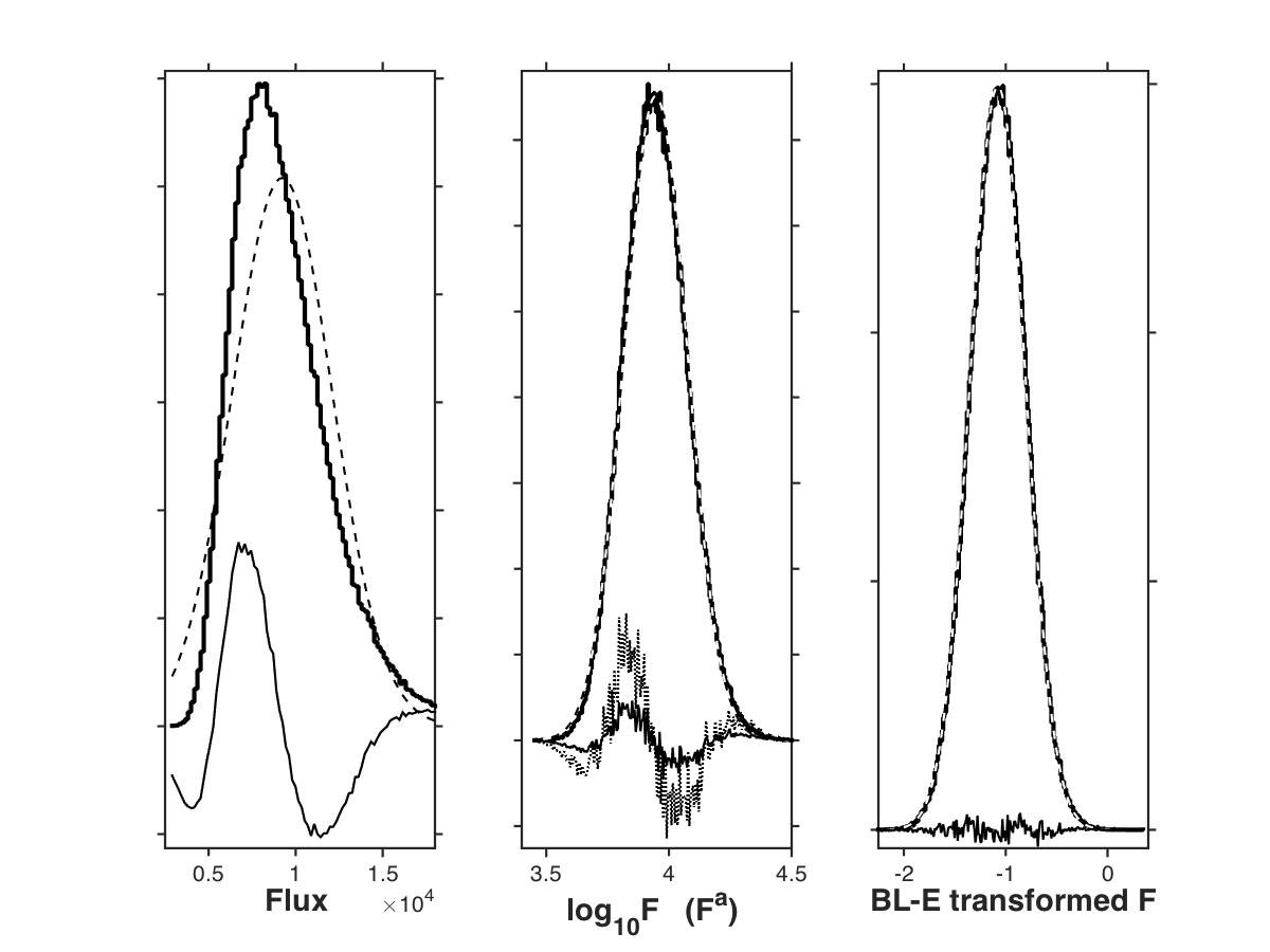
Figure 6: Cyg X-1 flux distributions (thick solid lines), best fitting normal functions (dashed lines) and residuals (thin lines). Left: raw fluxes. Middle: log and power law transformed fluxes (optimum $a=0.04$). For the latter the residuals (dotted line) are multiplied by 3 for clarity, but are essentially indistinguishable from those for the log transform. Right: Optimized Bar-Lev and Enis transform, with $\alpha=0.01$ and $\beta=0.664$.

7 Discussion

For several reasons the class of autoregressive/moving average and related processes discussed here form a powerful and flexible set of models for time series data observed in a variety of flickering astronomical sources.

Astrophysical realism: The curves plotted in Figure 1 are visually similar to time series data for many flickering astronomical sources, for example the gamma-ray light curves of the active galactic nuclei discussed by Meyer, Scargle and Blandford (2019). Even just these three samples suggest that the wide range of intermittency in the observations can be represented with innovations of varying degrees of sparsity. The degree of flare overlap, ranging from isolated discrete events to very considerable merging of the profiles of successive flares, is controlled by the distribution of the innovation. For modeling of actual time series data, if deterministic background trends, observational errors, and optimized parameters (flare shape and innovation) are incorporated, these sample simulations become even more realistic.

Implementation properties: The Wold Theorem and its constructive proof (Scargle, 1981b) both guarantee the existence of these linear and remarkably specific models for arbitrary stationary data, and provide a pathway to estimating them. Their second order statistics (power spectra and autocorrelation functions) are those of the event shape $C$, and therefore are essentially arbitrary – flexible enough to match the second order statistics of any time series data. The results derived here demonstrate that they can match flux distributions and rms-mean flux relations as well. The models fit the data exactly, so quality-of-fit resides in the statistical properties of the innovation. A great many theoretical properties of this class of random processes have been explored and supported by efficient algorithms, included in standard data analysis systems.

Physical Interpretation: The models have natural and useful interpretations. The moving average form embodies a random sequence of flares of various amplitudes. Flare shape and amplitude properties are separated, each leading to useful comparisons with physical theory. The autoregressive form explicates the standard short-term or long-term memory characteristics of Markov processes and random walks.

Are these models linear? Well, that depends on what you mean! Equation (4) has a clear linear input-output structure: if the innovation is a linear combination of two or more independent innovations, the output is a linear combination of the corresponding outputs. In addition, this equation represents memory – the Markov property – as a linear combination of prior values. The moving average/autoregressive model is linear in both of these senses.

A comprehensive development of analysis tools in this framework is left to another publication. The main purpose here is to clarify some methodological issues relevant to deriving physical properties of astronomical sources from statistical properties of their time series data. To wit: the following statistical properties can be derived from time series data: power spectra, phase spectra, rms-mean flux relations, flux distributions, measures of stationarity or intermittency, and dynamic range. In many publications these properties, separately or in combination, have been taken to imply that the observed system must (or must not) have, separately or in combination: non-linear dynamics, non-stationary time evolution, multiplicative component processes, or representability in terms of random flares (“shot noise”). The models discussed here serve as counterexamples to such assertions. Without any such physical properties these stationary, additive, linear random process models can generally speaking match the observations, e.g. by displaying linear dependence of flux standard deviation on flux mean and log-normal flux distribution.

This conclusion supports the view that the near ubiquity of relevant properties of light curves are likely statistical features that are generic, at least within the arena of astronomical time series, not necessarily associated with a universal physical mechanism. Specifically, mere stationarity is a sufficient condition for the existence of the relevant linear models, which have none of the exotic properties listed above.

Examples of the mistaken implications mentioned above are too many to cite in detail. A common assertion is that a linear rms-mean flux relation in the time series data implies non-linearity or non-stationarity of the physical process underlying the observed flickering. Also disproved are similar assertions about “shot noise,” such as that it must have, or must not have, certain features. In some cases this may be a semantic issue; if shot-noise is defined to have a stationary innovation, then it obviously cannot be non-stationary. But the flexibility of the distribution of the innovation allows either behavior. Assertions of the form

Given statistical property X, the underlying process must have property Y and cannot have property Z.

generally speaking should rather be phrased

Given statistical property X, the underlying process may have property Y (but there are simple models that do not have this property), evidence for which could be obtained from other considerations or other data. Regarding Z: Never say never.

What approaches can avoid the missteps cautioned against here? Careful attention to the definitions of the various time series statistics, and clearheaded evaluation of the astrophysical consequences of the corresponding observations, are obviously needed. Sophisticated or detailed models should be evaluated against the null hypothesis that simple (linear, additive and stationary) autoregressive/moving average models adequately represent the observations.

These models can provide direct information about variability duty cycles and the statistical distributions of flare amplitudes (through the innovation) and shapes (through the model coefficients). In addition, the formalism described here holds the promise of deriving physically meaningful properties of the underlying Markov process via values of $\alpha$ and $\beta$ in Equation (10). read off the RMS-mean flux relation. Toward this end, linkage of properties of the innovation and flare shapes to astrophysical characteristics would be useful. A specific example: asymmetric flares, such as fast rise and exponential decay (FRED), might indicate explosive injections followed by expansion and cooling, or delays across a curved relativistic jet front (Fenimore, Madras, and Nayakshin, 1996); symmetric flares might point toward jets randomly sweeping by the line of sight to the observer (Nemiroff, Norris, Kouveliotou, et al., 1994).

All of these approaches can profit from an openness to what generic physical characteristics are indeed implied by the observations, notwithstanding the cautions urged in this discussion. For example some of the conclusions that do not follow ineluctably from the statistical characteristics discussed in this note might be supported by auxiliary information – notably time resolved measurements of polarization and energy spectra.

Lastly, the model framework discussed here is far from the final word. Not all of issues affecting practical use of this class of models have been resolved. While the ambiguities related to causality and delay properties have been addressed via a generalization of the Wold Decomposition Scargle (1981a, b), there remains the obvious difficulty of flare shapes that depend on time, either systematically or randomly. Press (1978) discussed scale superimposition processes – moving averages in which the flare shape is stretched by a randomly varying factor. If the stretch process is stationary, the Wold Representation expresses the resulting time series as the superposition of a single fixed shape, which must somehow be an average of the stretched ones. The details of how this all works are not obvious.

8 Acknowledgements

Thanks especially to Sarah Wagner and Jay Norris for many useful for comments, and also to Krista Lynne Smith, Roger Romani, Paul Burd, Aneta Siemiginowska, Manuel Meyer, Javier Pascual-Granado, Rafael Garrido and the anonymous referee. Phil Uttley, and Simon Vaughan provided especially useful comments and suggestions. I am indebted to the NASA Astrophysics Data Analysis program for support through grant NNX16AL02G, as well as the NASA Applied Information Systems Research program.

References

- Alston, Fabian, Buisson et al. (2019) Alston, W., Fabian, A., Buisson, D., et al. 2019, The remarkable X-ray variability of IRAS 13224-3809 I. The variability process, MNRAS, 482, 2088-2106
- Alston (2019) Alston, W. 2019, Non-stationary variability in accreting compact objects, MNRAS, 485, 260-265
- Aschwanden (2011) Aschwanden, M. 2011, Self-Organized Criticality in Astrophysics: The Statistics of Nonlinear Processes in the Universe, Springer-Verlag, Berlin.
- Bar-Lev and Enis (1988) Bar-Lev, S. and and Enis, P. 1988, On the classical choice of variance stabilizing transformations and an application for a Poisson variate, Biometrica, 75, 803-804
- Bhatta and Dhital (2019) Bhatta, G. and Dhital, N. 2019, Nature of gamma-ray variability in blazars, arXiv: 1911.08198
- Box and Cox (1964) Box, G. E. P. and Cox, D. R. 1964, An analysis of transformations, Journal of the Royal Statistical Society, Series B, 26, 211-252.
- Brockwell and Davis (1987) Brockwell, P. and and Davis, R. 1987, Time Series: Theory and Methods, Springer-Verlag New York, Inc.
- Buchler and Kandrup (1997) Buchler, J. and Kandrup, H., eds.1997, Nonlinear Signal and Image Analysis, Vol. 808, Annals of the New York Academy of Sciences: New York
- Crow and Shimizu (1988) Crow, E. and Shimizu, K. 1988, Lognormal Distributions: Theory and Applications, Marcel Dekker, Inc.: New York
- Curtiss (1942) Curtiss, J.1942, On transformations used in the analysis of variance, Ann. Math. Statist., 14, 107-122
- Denis et al. (1994) Denis, W., Olive, J.-F., Roques, J. et al. 1994, Noise variability of the hard X-ray transient Nova Persei ApJS, 92, 459-463.
- Dobrotka and Ness (2015) Dobrotka, A. and Ness, J. 2015, Differences in the fast optical variability of the dwarf nova V1504 Cyg between quiescence and outbursts detected in Kepler data and simulations of the RMS-flux relations, MNRAS, 451, 2851
- Dobrotka, Negoro and Mineshige (2019) Dobrotka, A., Negoro, H., and Mineshige, S. 2019, Similar shot profile morphology of fast variability in cataclysmic variable, X-ray binary and blazar; the MVLyr case, arXiv: 1908.11745, to appear in A&A
- Eckmann and Ruelle (1992) Eckmann, J. and Ruelle, D. 1992, Fundamental limitations for estimating dimensions and Lyapunov exponents in dynamical systems, Physica D, 56, 185-187
- Edelson, Mushotzky, Vaughan et al. (2013) Edelson, R., Mushotzky, R., Vaughan, S., Scargle, J., Gandhi, P., Malkan, M., and Baumgartner, W. 2013, Kepler observations of rapid optical variability in the BL Lac object W2R1926+42, ApJ, 766, 16
- Efron (1982) Efron, B. 1982, Transformation Theory: How Normal is a Family of Distributions?, The 1981 Wald Memorial Lectures, Annals of Statistics, 10, 323-339
- Fenimore, Madras, and Nayakshin (1996) Fenimore, E., Madras, C., and Nayakshin, S. 1996, Expanding Relativistic Shells and Gamma-Ray Burst Temporal Structure, ApJ, 473, 998
- Giebels and Degrange (2009) Giebels, B. and Degrange, B. 2009, Lognormal variability in BL Lacertae (Research Note) A&A, 503, 797-799
- Granger and Anderson (1978) Granger, W. and Anderson, A. 1978, An Introduction to Bilinear Time Series Models, Vandenhoeck and Ruprecht: Göttingen
- Granger and Joyeux (1980) Granger, C. and Joyeux, R. 1980, An Introduction to Long Memory Time Series Models and Fractional Differencing, Journal of Time Series Analysis, 1, 15-30.
- Heil, Vaughan and Uttley (2012) Heil, L., Vaughan, S., and Uttley, P. 2012, The Ubiquity of the RMS-flux relation in Black Hole X-ray Binaries, MNRAS, 422, 2620
- Hogg and Reynolds (2016) Hogg, J. and Reynolds, C. 2016, Testing the Propagating Fluctuations Model with a Long, Global Accretion Disk Simulation, ApJ, 826, 40
- Kelly et al. (2009) Kelly, B., Bechtold, J., & Siemiginowska, A. 2009, Are the Variations in Quasar Optical Flux Driven by Thermal Fluctuations? ApJ, 698, 895
- Kelly, Sobolewska, and Siemiginowska (2011) Kelly, B., Sobolewska, M., and Siemiginowska, A. 2011, A Stochastic Model for the Luminosity Fluctuations of Accreting Black Holes, ApJ, 730, 52
- Kelly et al. (2014) Kelly, B., Becker, A, Sobolewska, M., et al. 2014, Flexible and Scalable Methods for Quantifying Stochastic Variability in the Era of Massive Time-Domain Astronomical Data Sets, ApJ, 788, 33
- Koen (2016) Koen, C. 2016, A simple explanation of the linear RMS-mean flux relation in accreting objects, A&A, 593, L17
- Kushwaha, Sinha, Misra, Kingh, and de Gouveia Dal Pino (2017) Kushwaha, P. Sinha, A., Misra, R. Singh, K., de Gouveia Dal Pino, E. 2017, Gamma-ray Flux Distribution and Non-linear behavior of Four LAT Bright AGNs, ApJ, 849, 138
- Lyubarskii (1997) Lyubarskii, Y. 1997, Flicker noise in accretion disks, MNRAS, 292, 679-685
- Meyer, Scargle and Blandford (2019) Meyer, M., Scargle, J. and Blandford, R. 2019, Characterizing the Gamma-Ray Variability of the Brightest Flat Spectrum Radio Quasars Observed with the Fermi LAT, ApJ, 877, 39.
- Mineshige, Ouchi and Nishimori (1994) Mineshige, S., Ouchi, N., and Nishimori, H. 1994, On the Generation of 1/f Fluctuations in X-Rays from Black-Hole Objects, Publ. Astron. Soc. Japan, 46, 97-105
- Nemiroff, Norris, Kouveliotou, et al. (1994) Nemiroff, R., Norris, J., Kouveliotou, C., Fishman, G., Meegan, C., and Paciesas, W. 1994, Gamma-Ray Bursts are Time-Asymmetric ApJ423, 432
- Osborne and Provenzale (1989) Osborne, A. and Provenzale, A. 1989, Finite correlaiton dimension for stochastic systems with power-law spectra, Physica D 47, 361-372
- Parzen (1962) Parzen,E., Spectral analysis of asymptotically stationary time series, Bull. Inst. Internat. Statist., 39, 87-2013, 1962
- Pascual-Granado, Garrido and Suárez (2013) Pascual-Granado, J., Garrido, R., Suárez, J. 2013, On the necessity of a new interpretation of the stellar light curves, Proceedings of the IAU, Vol. 9, S301, 2013, pp 85-88 arXiv:1311.3553
- Pascual-Granado, Garrido and Suárez (2015) Pascual-Granado, J., Garrido, R., Suárez, J. 2015, Inconsistencies in the application of harmonic analysis to pulsating stars, Astronomy and Astrophysics, 581, A89, arXiv:1507.07877
- Phillipson, Boyd and Smale (2018) Phillipson, R., Boyd, P. and Smale, A. 2018, The Chaotic Long-term X-ray Variability of 4U 1705-44, MNRAS, 477, 5220-5237
- Press (1978) Press, W.1978, Flicker Noise in Astronomy and Elsewhere, Comments Astrophys, 7, 103-119.
- Priestley (1988) Priestley, M. 1988, Non-linear and Non-Stationary Time Series Analysis, Academic Press: New York
- Ruelle (1990) Ruelle, D. 1990, Deterministic chaos: the science and the fiction, The Claude Bernard Lecture, 1989, Proc. R. Soc. Lond. A, 427, 241-248
- Scargle (1981a) Scargle, J. 1981a, Phase-sensitive deconvolution to model random processes, with special reference to astronomical data, 1981, In Applied Time Series Analysis II, D. Findley ed. New York: Academic Press.
- Scargle (1981b) Scargle, J. 1981b, Studies in Astronomical Time Series Analysis: I. Modeling Random Processes in the Time Domain, ApJS, 45, 1
- Scargle, Donoho, Crutchfield et al. (1992) Scargle, J., Donoho, D., Crutchfield, J., Steiman-Cameron, T., Imamura, J., and K. Young, K. 1993, The Quasi-Periodic Oscillations and Low-Frequency Noise of Scorpius X-1 as Transient Chaos; A Dripping Handrail?, Astrophysical Journal Letters, 411, L91-L94.
- Scaringi et al. (2012) Scaringi, S., Körding, Uttley, P., Knigge, C., Groot, P. and Still, M. 2012, The Universal Nature of Accretion-induced Variability: the RMS-Flux Relation in an Accreting White Dwarf, MNRAS, 421, 2854
- Shah et al. (2018) Shah, Z., Mankuzhiyil, N., Sinha, A., Misra, R., Sahayanathan, S., and Iqbal, N. 2018, Log-normal flux distribution of bright Fermi blazars, Research in Astronomy and Astrophysics, 18, 141
- Sinha, Khatoon, Mistra at al. (2018) Sinha, A., Khatoon, R., Misra, R., Sahayanathan, S. Mandal, S., Gogoi, R., Bhatt, N. 2018, The flux distribution of individual blazars as a key to understand the dynamics of particle acceleration, MNRAS Letters, 480, L 116-120
- Smith et al. (2018) Smith, K., Mushotzky, R., Boyd, P., Malkan, M., Howell, S. and Gelino, D. 2018, The Kepler Light Curves of AGN: A Detailed Analysis, ApJ, 857, 141
- Sprott (2003) Sprott, J. 2003, Chaos and Time-Series Aanalysis, Oxford University Press, Oxford
- Takata, Mukuto and Mizumoto (2018) Takata,T., Mukuta, Y, and Mizumoto, Y. 2018, Modeling the Variability of Active Galactic Nuclei by an Infinite Mixture of Ornstein-Uhlenbeck (OU) Processes, ApJ, 869, 178 [Erratum: 2018, ApJ, 869, 178]
- Theiler, Lindday and Rubin (1993) Theiler, J., Lindday, P. and Rubin, D. 1993, Detecting Nonlinearity in Data with Long Coherence Times, in Predicting the Future and Understanding the Pose, Eds. Weigent, A. and Gerschenfeld, N., SFI Studies in the Sciences of Complexity, Proc. Vol. XVII, Addison-Wesley,
- Thorne and Blandford (2017) Thorne, K. and Blandford, R. 2017, Modern Classical Physics, Princeton University Press
- Tong (1990) Tong, H. 1990, Non-linear Time Series: A Dynamical System Approach, Clarendon Press: Oxford
- Uttley and McHardy (2001) Uttley, P., and McHardy, I., 2001, The flux-dependent amplitude of broadband noise variability in X-ray binaries and active galaxies, MNRAS 323, L26.
- Uttley et al. (2005) Uttley, P., McHardy, I., and Vaughan, S. 2005, Non-linear X-ray variability in X-ray binaries and active galaxies, MNRAS, 359, 345-362
- Uttley, McHardy and Vaughan (2017) Uttley, P., McHardy, I., and Vaughan, S. 2017, The RMS-flux relation in accreting objects: not a simple ”volume control,” A&A, 601, 1
- Vaughan and Uttley (2008) Vaughan, S. and Uttley, P. 2008, Studying accreting black holes and neutron stars with time series: beyond the power specrum, “Noise and Fluctuations,” Proc. SPIE, 6603
- Vaughan (2013) Vaughan, S. 2013, Random time series in Astronomy, Phil. Trans. R. Soc. A, 1-28
- Wold (1938) Wold, Herman O. A. 1938, A Study in the Analysis of Stationary Time Series, Almqvist & Wiksells: Uppsala
- Young and Scargle (1996) Young, K. and Scargle, J. 1996, The Dripping Handrail Model: Transient Chaos in Accretion Systems ApJ, 468, 617
- Yule (1926) Yule, G. 1926, Why do we Sometimes get Nonsense Correlations between Time Series? – A Study in Sampling and the Nature of Time-Series, Journal of the Royal Statistical Society, 89, 1-63.