Bayesian design for minimising prediction uncertainty in bivariate spatial responses with applications to air quality monitoring

ABSTRACT

Model-based geostatistical design involves the selection of locations to collect data to minimise an expected loss function over a set of all possible locations. The loss function is specified to reflect the aim of data collection, which, for geostatistical studies, could be to minimise the prediction uncertainty at unobserved locations. In this paper, we propose a new approach to design such studies via a loss function derived through considering the entropy about the model predictions and the parameters of the model. The approach also includes a multivariate extension to generalised linear spatial models, and thus can be used to design experiments with more than one response. Unfortunately, evaluating our proposed loss function is computationally expensive so we provide an approximation such that our approach can be adopted to design realistically sized geostatistical studies. This is demonstrated through a simulated study and through designing an air quality monitoring program in Queensland, Australia. The results show that our designs remain highly efficient in achieving each experimental objective individually, providing an ideal compromise between the two objectives. Accordingly, we advocate that our approach could be adopted more generally in model-based geostatistical design.

Keywords: Bivariate response models, Copula models, Entropy, Generalised linear spatial models, Spatial dependence.

1  Introduction

The importance of spatial dynamics in natural processes has become a major focus of enquiry in many fields including ecology, agriculture and marine biology (Bloom and Kentwell, 1999; Bruno et al., 2001; Castrignanò et al., 2008; Falk et al., 2014). Often, what can be explored and ultimately inferred about such dynamics depends on how the data were collected, and, in particular, the specific locations in space (Müller, 2007). In this paper, we propose an approach in Bayesian design for selecting sampling locations to efficiently learn about the spatial dynamics underpinning natural processes. In particular, we focus on quantifying and minimising uncertainty about model predictions at unobserved locations which simultaneously provides precise estimates of model parameters.

One common approach to modelling spatial dynamics is via a Gaussian process model (Diggle et al., 2003). Such a model assumes that the observations can be regarded as a realisation from a Gaussian process $\{S(\mathbold{d});\mathbold{d}\in\Re^{2}\}$. Typically, $S(\cdot)$ is assumed to be stationary and isotropic with mean identically equal to zero and covariance function $\text{Cov}(h)=\text{Cov}(S(\mathbold{d}),S(\mathbold{d}^{{}^{\prime}}))$ where $h=||\mathbold{d}-\mathbold{d}^{{}^{\prime}}||$ is the Euclidean distance between locations $\mathbold{d}$ and $\mathbold{d}^{{}^{\prime}}$. For ease of notation, the $i$th observation $S(\mathbold{d}_{i})$, where $\mathbold{d}_{i}$ is the location of the $i$th observation, will be abbreviated to $s_{i}$ throughout this article. Through such a model, one can then leverage information about the spatial variability between locations to yield predictions at unobserved locations.

Bayesian inference provides a rigorous framework to quantify and handle uncertainty in spatial predictions, and a number of authors have considered this framework to design geostatistical studies. The work of Diggle and Lophaven (2006) compared the prediction performance of different classes of designs such as the ‘lattice plus close pairs’ and ‘lattice plus in-fill’ designs under parameter uncertainty. As such, no optimisation of the design was undertaken. This is presumably because of the large computational time involved in evaluating their loss function, and this is typical of designs for prediction. A pseudo-Bayesian design approach was proposed by Falk et al. (2014) for sampling on stream networks. Optimal designs were found under various loss functions but their work was limited to assuming some or all parameter values were known a priori. Bayesian approaches to design monitoring networks were proposed by Müller et al. (2004) and Fuentes et al. (2007) such that accurate predictions could be obtained while minimising the cost of monitoring. However, both approaches do not take into account parameter uncertainty. Further, to form a dual-objective loss function, both approaches considered a linear combination of loss functions which requires specifying the relative importance of each objective via pre-defined weights. Unfortunately, such an approach has been shown to be difficult to apply in practice (Hill et al., 1968; Cook and Wong, 1994; McGree et al., 2008). For a similar purpose, Le et al. (2003) proposed an entropy-based criterion for designing networks for monitoring multivariate environmental fields. However, their approach can only be applied to network problems where the responses are approximately normally distributed, and hence has limited applicability.

Across all of the design methods proposed in the above cited papers, only a limited number of approaches have taken into account both parameter uncertainty and the uncertainty in the predicted outcomes when assessing a design. This is potentially a major limitation as both sources of uncertainty could be significant. Further, most of these approaches were limited to consider spatially dependent univariate responses or multivariate responses that are marginally Gaussian. This is potentially because of the difficulty in constructing a multivariate distribution that appropriately describes the dependencies between each response. As each response may be of a different type (i.e. continuous, count, binary, etc), this can lead to a rather complex model, rendering many approaches in Bayesian design computationally infeasible. Such a limitation seems rather restrictive as multiple responses are often observed in geostatistical studies e.g. Bohorquez et al. (2017); Musafer and Thompson (2017).

To address the limitations of previous research, we consider a generalised linear spatial modelling (GLSM) framework where the dependence between responses is described by a Copula model. Such functions are defined based on the cumulative distribution function (CDF) of the univariate responses, meaning that the joint distribution can be defined for a variety of different data types. Then, given such a model, we propose to quantify the uncertainty in spatial predictions via an entropy-based loss function. The benefit of this is that one can then exploit the additivity property of entropy, avoiding the need to pre-specify weights on different objectives like estimation and prediction. To demonstrate our approach, we design a simulated study and also an air quality monitoring program in Queensland, Australia, and assess the performance of the resulting designs.

This paper is outlined as follows. In Section 2, the GLSM framework for modelling spatial outcomes is defined, and the Copula representation for describing multivariate spatial data is introduced. Our Bayesian design framework is described in Section 3, along with our approach to quantify and minimise uncertainty in model predictions. In doing so, we show how such an approach also minimises uncertainty about parameter estimates, and provide an approximation to efficiently evaluate this loss function. To illustrate our methodologies, Section 4 focuses on finding designs in two examples where bivariate mixed spatial outcomes are observed. The paper concludes with a discussion of key findings and suggestions for future research.

2  Motivating example

Exposure to high levels of air pollution can have a variety of adverse effects on human health, including respiratory infections, heart disease, and lung cancer (Watson, 2006; Jiang et al., 2016; Zhang et al., 2016). This has led to an initiative by the Queensland government in Australia to monitor air quality across the state to provide information for managing and ultimately reducing air pollution. Key indicators of air quality that are measured across the state include $NO_{2}$ and $PM_{2.5}$ concentrations which are known to have significant adverse effects on human health (Roberts et al., 2019; Huang et al., 2019). However, such monitoring is hugely expensive, particularly in terms of setting up and maintaining the monitoring stations. Consequently, there is recent interest in exploring the impact of reduced sampling across the network, and how this might affect regulator’s ability to predict air pollution at unsampled locations of interest. This provides motivation for the research proposed in this paper where a retrospective sampling design is sought across the current network of air quality monitoring stations in Queensland.

2.1  Available data

The Queensland air quality monitoring network consists of 22 monitoring stations; seven of which measure both $NO_{2}$ and $PM_{2.5}$ concentrations. Figure 1 shows the spatial configuration of these 22 stations where we will refer to stations that measure both $NO_{2}$ and $PM_{2.5}$ concentrations as “sampled” locations and stations that do not measure both of these concentrations as “unsampled” locations.

For the sampled locations, the annual mean $NO_{2}$ concentrations ($Y_{1}$), the number of days (per annum) which exceed the daily $PM_{2.5}$ limit of $10{\mu}gm^{-3}$ ($Y_{2}$), and meteorological data from year 2013 to 2016 were sourced from the Queensland government website (https://data.qld.gov.au/dataset). These data were then used to develop a generalised linear spatial model to describe the observed variability in both pollutants. This model was then used to inform the selection of proposed monitoring stations within the retrospective design.

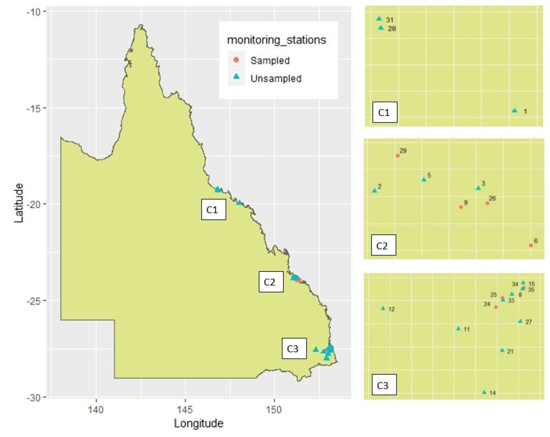
Figure 1: The locations of the selected air quality monitoring stations

3  Modelling bivariate responses in a geostatistical study

In this section, we describe our modelling framework for bivariate responses collected in a geostatistical study. We start by first describing how a univariate response could be modelled, then extend to bivariate responses.

3.1  Spatial model for a univariate response

To model a univariate response collected in a geostatistical study, we consider a GLSM which has the following form:

$${\mu_{i}}=\mathbold{X}_{i}^{T}\mathbold{\beta}+s_{i}\hskip 14.22636pt\text{and}\hskip 14.22636ptE({y_{i}|s_{i}})=g^{-1}(\mu_{i}),\;\text{for}\;i=1,2,\ldots,n,$$

where $\mathbold{X}_{i}=(1,X_{i1},\ldots,X_{ip-1})^{T}$ is the covariate vector associated with the location $\mathbold{d}_{i}$, $\mathbold{\beta}\in\Re^{p}$ are the regression coefficients (fixed effects), and ${s_{i}}$ is the value of the $i$th random effect. Here, the link function $g(.)$ defines the relationship between the linear predictor ${\mu_{i}}$ and the expected outcome given $s_{i}$.

In a GLSM, conditional on the random effects, the dependent variable $Y$ follows a distribution from the exponential family. The joint distribution of the random effects $s_{1},s_{2},\ldots,s_{n}$ is assumed to be Multivariate Normal with mean vector zero and covariance matrix $\mathbold{\Sigma}$. When formulating this covariance matrix, it is convenient to consider a specific parametric family of covariance functions (Albert and McShane, 1995; Diggle et al., 2003). In this paper, the Matérn covariance function is used, and has the following form:

$$\text{Cov}(h;\mathbold{\gamma},\nu)=\gamma_{1}\rho(h,\gamma_{2},\nu)\;\text{and}\;\rho(h;\gamma_{2},\nu)=\frac{1}{2^{\nu-1}\Gamma(\nu)}\big{(}h/\gamma_{2}\big{)}^{\nu}K_{\nu}(h/\gamma_{2}),$$

where $\nu>0$, $\mathbold{\gamma}=(\gamma_{1},\gamma_{2})$ and $h$ is the Euclidean distance between two locations. $\Gamma(\cdot)$ is the gamma function and $K_{\nu}(\cdot)$ is the modified Bessel function of order $\nu$. The parameters $\gamma_{1}$ and $\gamma_{2}$ are the partial sill and the spatial range, respectively. Here, we define the covariance function at the linear predictor level. Additional variability will be assumed at the data level, the form of which will depend on the data type.

To describe a Bayesian framework for the above model, let $\mathbold{y}_{i}=(y_{i1},\ldots,y_{in_{i}})^{T}$ denote the observed data at location $\mathbold{d}_{i}$ where $n_{i}$ is the number of observations collected at location $\mathbold{d}_{i}$, for $i=1,\ldots,n$. In spatial design, the design $\mathbold{d}=(\mathbold{d}_{1},\ldots,\mathbold{d}_{n})^{T}\in\mathscr{D}$ represents the locations where the outcomes $\mathbold{y}=(\mathbold{y}_{1},\ldots,\mathbold{y}_{n})^{T}$ are measured, and $\mathscr{D}$ represents the design space for the study. Let $p(\mathbold{\theta})$ denote the prior distribution about the parameters $\mathbold{\theta}$. Then, within a Bayesian framework, all inferences are based on the posterior distribution defined as follows:

$$p(\mathbold{\theta|y,d})\propto{\int\limits_{\mathbold{s\in S}}\prod\limits_{i=1}^{n}\prod\limits_{j=1}^{n_{i}}p(y_{ij}|\mathbold{d}_{i},s_{i},\mathbold{\beta})p(\mathbold{s|\gamma},\nu)p(\mathbold{\theta})\text{d}\mathbold{s}},$$

where $\mathbold{s}=(s_{1},\ldots,s_{n})^{T}$ is vector of random effects, and the parameter vector $\mathbold{\theta}$ includes both model parameters $\mathbold{\beta}$ and covariance parameters $\mathbold{\gamma}$ and $\nu$. $p(y_{ij}|\mathbold{d}_{i},s_{i},\mathbold{\beta})$ is the conditional likelihood of observing $y_{ij}$ at location $\mathbold{d}_{i}$ given the model parameters $\mathbold{\beta}$ and random effects $s_{i}$ for $i=1,\ldots,n$ and $j=1,\ldots,n_{i}$.

To extend the above model to handle bivariate responses, we consider Copula models to describe the dependence between responses (Nelsen, 2006; Bárdossy, 2006; Kazianka and Pilz, 2011; Gräler and Pebesma, 2011) (see next section). Adopting such an approach provides a framework to flexibly model dependence between bivariate responses.

3.2  Spatial model for bivariate responses

Here, we define a modelling approach for bivariate spatial responses by combining the univariate spatial models (defined above) via a suitable Copula model. For this, assume that two response variables will be observed with one being continuous $Y_{1}$ and the other being discrete $Y_{2}$; thus marginally they can be modelled via two GLSMs as follows:

$${\mu_{1i}}=\mathbold{X}_{i}^{T}\mathbold{\beta}_{1}+s_{1i},\hskip 5.69046ptE({y_{1i}|s_{1i}})=g_{1}^{-1}(\mu_{1i}),\hskip 5.69046pt\text{and}$$

$${\mu_{2i}}=\mathbold{X}_{i}^{T}\mathbold{\beta}_{2}+s_{2i},\hskip 5.69046ptE({y_{2i}|s_{2i}})=g_{2}^{-1}(\mu_{2i})\;\text{for}\;i=1,2,\ldots,n.$$

We assume that $Y_{1}$ and $Y_{2}$ have marginal probability distributions $f_{Y_{1}|s_{1i}}$ and $f_{Y_{2}|s_{2i}}$ given the random effects $s_{1i}$ and $s_{2i}$, respectively. Further, denote the marginal cumulative distribution function of $Y_{1}|s_{1i}$ and $Y_{2}|s_{2i}$ as $F_{Y_{1}|s_{1i}}$ and $F_{Y_{2}|s_{2i}}$, respectively. Then, the Copula representation of the joint distribution $G_{Y_{1}|s_{1i},Y_{2}|s_{2i}}$ is given by,

$$\begin{split}G_{Y_{1}|s_{1i},Y_{2}|s_{2i}}(y_{1ij},y_{2ij})&=C\big{(}F_{Y_{1}|s_{1i}}(y_{1ij}),F_{Y_{2}|s_{2i}}(y_{2ij});\alpha\big{)}\\ &=C(u_{1ij},u_{2ij};\alpha)\;\text{for}\;i=1,2,\ldots,n\;\text{and}\;\text{for}\;j=1,2,\ldots,n_{i},\end{split}$$

where $C$ and $\alpha$ denote the Copula function and the Copula parameter, respectively. The Copula parameter $\alpha$ defines the strength of dependence within the bivariate distribution (Nelsen, 2006).

From this, the Copula representation of the joint distribution of $Y_{1}|s_{1i}$ and $Y_{2}|s_{2i}$ is given by,

$$f_{Y_{1}|s_{1i},Y_{2}|s_{2i}}(y_{1ij},y_{2ij})=f_{Y_{1}|s_{1i}}(y_{1ij})(c_{1ij}-c_{1ij}^{*}),$$ (1)

where $c_{1ij}=\frac{\partial C(u_{1ij},u_{2ij};\alpha)}{\partial{u_{1ij}}}$ , $c_{1ij}^{*}=\frac{\partial C(u_{1ij},u_{2ij}^{-};\alpha)}{\partial{u_{1ij}}}$ and ${u_{2ij}^{-}}$ is the left hand limit of $u_{2ij}$, see Joe (2014) and Tao et al. (2013) for further details.

Then, using Equation (1), the conditional likelihood of a bivariate mixed outcome $(\mathbold{y}=({y_{1ij},y_{2ij}})$ for $i=1,2,\ldots,n\;\text{and}\;j=1,2,\ldots,n_{i})$ can be expressed as follows:

$$p(\mathbold{y|d},\mathbold{\theta},\mathbold{s}_{1},\mathbold{s}_{2})=\prod\limits_{i=1}^{n}\prod\limits_{j=1}^{n_{i}}\Big{[}\big{(}f_{Y_{1}|s_{1i}}(y_{1ij})\big{)}\big{(}c_{1ij}-c_{1ij}^{*}\big{)}\Big{]},$$

where $\mathbold{\theta}$ includes all the model parameters ($\mathbold{\beta}_{1},\mathbold{\beta}_{2}$), the covariance parameters ($\mathbold{\gamma}_{1}=(\gamma_{11},\gamma_{21}),$ $\mathbold{\gamma}_{2}=(\gamma_{21},\gamma_{22}),\nu_{1},\nu_{2}$), and the Copula parameter $\alpha$.

The bivariate Copula function describes the dependence structure between two random variables. A large number of bivariate Copulas and their dependence properties have been discussed in the literature (Durante and Sempi, 2010; Genest and MacKay, 1986; Nelsen, 2006). Among them, the bivariate Archimedean Copula models such as Clayton, Gumbel and Frank Copulas have been widely used due to their flexibility in describing different tail behaviours and different dependence structures.

The Clayton Copula is considered in this paper to model the joint distribution of the responses with the reader referred to Clayton (1978) and Cook and Johnson (1981) for further details. Let $Y_{1}$ and $Y_{2}$ be two responses with CDFs $u_{1}=F_{Y_{1}}(y_{1})$ and $u_{2}=F_{Y_{2}}(y_{2})$, respectively, then the joint CDF of $Y_{1}$ and $Y_{2}$ can be expressed using the Clayton Copula as follows:

$$C(u_{1},u_{2};\alpha)=({u_{1}}^{-\alpha}+{u_{2}}^{-\alpha}-1)^{-1/\alpha};\hskip 14.22636pt\alpha>0,$$

where $\alpha$ is the Copula parameter.

The choice of this Copula model was motivated by the tail dependence structure of the data observed in the motivating example and desirable properties of the Archimedean Copula family to which this Copula belongs. For example, as provided by Genest and MacKay (1986), there is a closed form relationship between the bivariate Archimedean Copula parameter and Kendall’s tau ($\tau$). Therefore, once the Copula parameter is estimated, it is straightforward to define the dependence between the two responses within the intuitive scale of $-1$ to $+1$. For example, the relationship between the Clayton Copula parameter $\alpha$ and Kendall’s tau can be defined as follows:

$$\tau=4E[C(u_{1},u_{2};\alpha)]-1=\frac{\alpha}{\alpha+2}.$$

4  Bayesian design framework for geostatistical studies

Our aim of minimising the uncertainty in spatial predictions can be quantified within a Bayesian design framework by a loss function which we will denote as $\lambda(\mathbold{d,\theta,y})$. Such a loss function compares a summary of the posterior distribution for $\mathbold{\theta}$ (based on observing $\mathbold{y}$ from $\mathbold{d}$) with its true value. However, as this function depends on $\mathbold{\theta}$ and $\mathbold{y}$, which are unknown a priori, it cannot be used to select designs. Accordingly, the expectation of the loss function is used to locate designs, and this expectation can be defined as follows:

$$L(\mathbold{d})=E_{\mathbold{y,\theta}}[\lambda(\mathbold{d,\theta,y})]=\int\limits_{\mathbold}{Y}\int\limits_{\mathbold}{\Theta}\lambda(\mathbold{d,\theta,y})p(\mathbold{y|\theta,d})p(\mathbold{\theta})\text{d}\mathbold{\theta}\text{d}\mathbold{y},$$ (2)

where $p(\mathbold{y}|\mathbold{\theta,d})=\int\limits_{\mathbold{s}\in\mathbold{S}}p(\mathbold{y}|\mathbold{\beta,s,d})p(\mathbold{s}|\mathbold{\gamma},\nu)d\mathbold{s}$.

When the loss function does not depend on the model parameters $\mathbold{\theta}$, Equation (2) can alternatively be expressed as:

$$L(\mathbold{d})=E_{\mathbold{y}}[\lambda(\mathbold{d,y})]=\int\limits_{\mathbold}{Y}\lambda(\mathbold{d,y})p(\mathbold{y|d})\text{d}\mathbold{y}.$$ (3)

A Bayesian design is then found by minimising the expected loss over the space of all possible locations. However, in general, the expected loss function does not have a closed-form solution, and hence, needs to be approximated. Monte Carlo (MC) integration is the most commonly used approach for this approximation. This is achieved by simulating a large number of prior predictive data sets, evaluating the loss function for each data set, and then taking the average as the approximation to the expected loss. Formally:

$$\hat{L}(\mathbold{d})={\frac{1}{K}}\sum\limits_{k=1}^{K}\lambda(\mathbold{d},\mathbold{\theta}_{k},\mathbold{y}_{k}),$$ (4)

where $\mathbold{\theta}_{k}$ and $\mathbold{y}_{k}$ are generated from the distributions $p(\mathbold{\theta})$ and $p(\mathbold{y}|\mathbold{d},\mathbold{\theta}_{k})$, respectively.

The current approach to Bayesian design for spatial prediction is based on a loss function proposed in Diggle and Lophaven (2006). This loss function quantifies the spatially averaged prediction variance of the unobserved random field $S(\cdot)$ over the predicted region $\mathscr{A}$ as follows:

$$\lambda_{pred}(\mathbold{d,y})=\int\limits_{\mathbold{\xi}\in\mathscr{A}}{\text{Var}\{S(\mathbold{\xi})|\mathbold{y,d}\}}\text{d}\mathbold{\xi}.$$ (5)

When the prediction region $\mathscr{A}$ consists a discrete set of locations $\mathbold{\xi}_{1},\mathbold{\xi}_{2},\ldots,\mathbold{\xi}_{T}$, the above loss function can be expressed as follows:

$$\lambda_{pred}(\mathbold{d,y})=\frac{1}{T}\sum\limits_{t=1}^{T}{\text{Var}\{S(\mathbold{\xi}_{t})|\mathbold{y,d}\}}.$$

As discussed in Diggle and Lophaven (2006), this loss function provides some provision to also address the objective of parameter estimation. In the next section, we describe an alternative approach for addressing these dual objectives.

4.1  An entropy-based loss function for spatial prediction

Here, we derive a loss function to quantify uncertainty in a spatial process by considering the entropy about the predictions, following the principles outlined in the seminal book by Le and Zidek (2006). For this, we note that, for a given model, there are two sources of uncertainty about the predictions: (1) Uncertainty in the parameter values; and (2) Uncertainty in the outcome $\mathbold{Z}$ conditional on the parameter values. Thus, to derive this loss function, we start by considering the entropy in these two random variables a priori. Initially we consider a univariate outcome $\mathbold{Z}$ where the entropy about this random variable and the parameter values is:

$$\begin{split}H(\mathbold{Z,\theta|\xi})=-\int\limits_{\mathbold{z}\in\mathcal{Z}}\int\limits_{\mathbold{\Theta}}p(\mathbold{z,\theta|\xi})\log p(\mathbold{z,\theta|\xi})\text{d}\mathbold{\theta}\text{d}\mathbold{z},\;\text{and}\\ H(\mathbold{Z,\theta|\xi})=-\sum\limits_{\mathbold{z}\in\mathcal{Z}}\int\limits_{\mathbold{\Theta}}p(\mathbold{z,\theta|\xi})\log p(\mathbold{z,\theta|\xi})\text{d}\mathbold{\theta},\end{split}$$

for cases where $\mathbold{Z}$ is a continuous and discrete outcome, respectively.

Following this, we define the loss function in terms of the change in entropy about $\mathbold{Z}$ and the parameters upon observing data $\mathbold{y}$ at design $\mathbold{d}$ as follows:

$$\lambda_{D}(\mathbold{d,y})=H(\mathbold{Z,\theta|y,d,\xi})-H(\mathbold{Z,\theta|\xi}),$$ (6)

where $H(\mathbold{Z,\theta|y,d,\xi})$ is the entropy about $\mathbold{Z}$ and the parameters upon observing data $\mathbold{y}$ at design $\mathbold{d}$.

Using the chain rule of entropy, it is straightforward to show that the joint entropy of $\mathbold{Z}$ and the parameters is equal to the conditional entropy of $\mathbold{Z}$ given the parameters plus the entropy of the parameters. That is:

$$\begin{split}H(\mathbold{Z,\theta|y,d,\xi})=H(\mathbold{Z|\theta,y,d,\xi})+H(\mathbold{\theta|y,d}),\;\text{and}\;H(\mathbold{Z,\theta|\xi})=H(\mathbold{Z|\theta,\xi})+H(\mathbold{\theta}),\end{split}$$ (7)

where, when $\mathbold{Z}$ is a discrete random variable, $H(\mathbold{Z|\theta,\xi})=-\sum\limits_{\mathbold{z}\in\mathcal{Z}}\int\limits_{\mathbold{\Theta}}p(\mathbold{z,\theta|\xi})\log\frac{p(\mathbold{z,\theta|\xi})}{p(\mathbold{\theta})}\text{d}\mathbold{\theta}$ and $H(\mathbold{\theta})=-\int\limits_{\mathbold{\Theta}}p(\mathbold{\theta})\log{p(\mathbold{\theta})}\text{d}\mathbold{\theta}$.

Then, by substituting the above expressions into Equation (6), the loss function $\lambda_{D}(\mathbold{d,y})$ can be expressed as follows:

$$\begin{split}\lambda_{D}(\mathbold{d,y})&=H(\mathbold{Z,\theta|y,d,\xi})-H(\mathbold{Z,\theta|\xi})\\ &=\big{\{}H(\mathbold{Z|\theta,y,d,\xi})+H(\mathbold{\theta|y,d})\big{\}}-\big{\{}H(\mathbold{Z|\theta,\xi})+H(\mathbold{\theta})\big{\}}\\ &=\big{\{}H(\mathbold{Z|\theta,y,d,\xi})-H(\mathbold{Z|\theta,\xi})\big{\}}+\big{\{}H(\mathbold{\theta|y,d})-H(\mathbold{\theta})\big{\}}\\ &=\lambda_{P}(\mathbold{d,y})+\lambda_{E}(\mathbold{d,y}).\end{split}$$ (8)

As shown in Equation (8), the loss function $\lambda_{D}(\mathbold{d,y})$ can be expressed as a sum of two loss functions in which the first ($\lambda_{P}(\mathbold{d,y})$) quantifies the change in entropy about $\mathbold{Z}$ given the parameters $\mathbold{\theta}$ while the second ($\lambda_{E}(\mathbold{d,y})$) quantifies the change in entropy about the parameter values. Thus, the loss function $\lambda_{D}(\mathbold{d,y})$ is termed as a dual-purpose loss function for parameter estimation and prediction. The derivation of Equation (8) is essentially the same as the fundamental identity given in Le and Zidek (2006).

For parameter estimation, the loss function $\lambda_{E}(\mathbold{d,y})$ is equivalent to the Kullback-Leibler divergence (KLD) between the prior and the posterior distributions of parameters (Kullback and Leibler, 1951), and can be expressed as follows:

$$\lambda_{E}(\mathbold{d,y})=-\int\limits_{\mathbold}{\Theta}{p(\mathbold{\theta|y,d})}\log\Bigg{(}\frac{p(\mathbold{\theta|y,d})}{p(\mathbold{\theta})}\Bigg{)}\text{d}\mathbold{\theta}.$$ (9)

When comparing designs via the loss function $\lambda_{P}(\mathbold{d,y})$, the term $H(\mathbold{Z|\theta,\xi})$ is independent of the design $\mathbold{d}$. As such, for simplicity, we consider $H(\mathbold{Z|\theta,y,d,\xi})$ as our loss function for prediction given the parameters as follows:

$$\lambda_{P}(\mathbold{d,y})=H(\mathbold{Z|\theta,y,d,\xi})=-\int\limits_{\mathbold{\Theta}}p(\mathbold{\theta|y,d})\sum\limits_{\mathbold{z}\in\mathcal{Z}}p(\mathbold{z|\theta,y,d,\xi})\log p(\mathbold{z|\theta,y,d,\xi})\text{d}\mathbold{\theta}.$$ (10)

However, when assessing the performance of designs under this expected loss, the term $H(\mathbold{Z|\theta,\xi})$ is subtracted so that the resulting values are interpretable.

When a bivariate mixed outcome (i.e. one outcome is continuous and the other is discrete) is observed ($\mathbold{z}=(\mathbold{z_{1},z_{2}})$), the above loss function can be expressed as follows:

$$\lambda_{P}(\mathbold{d,y})=-\int\limits_{\mathbold{\Theta}}p(\mathbold{\theta|y,d})\sum\limits_{\mathbold{z_{2}}\in\mathcal{Z}_{2}}\int\limits_{\mathbold{z_{1}}\in\mathcal{Z}_{1}}{p(\mathbold{z_{1},z_{2}|\theta,y,d,\xi})}{\log p(\mathbold{z_{1},z_{2}|\theta,y,d,\xi})}\text{d}\mathbold{z_{1}}\text{d}\mathbold{\theta},$$ (11)

where $\mathbold{y}=(\mathbold{y_{1},y_{2}})$ contains data collected for the two responses at the locations $\mathbold{\xi}$ based on design $\mathbold{d}$.

The loss function $\lambda_{E}(\mathbold{d,y})$ for the bivariate mixed outcome is defined as above, where $\mathbold{\theta}$ contains all model parameters for both responses.

5  Efficient approximations to loss functions

Evaluating the MC approximation to the expected loss in Equation (11) requires approximating or sampling from a large number of posterior distributions. Unfortunately, this renders algorithms like Markov chain Monte Carlo computationally infeasible to use in locating designs. Accordingly, in this section, we describe computationally efficient methods for approximating the above loss functions.

5.1  Approximating the posterior distribution

To efficiently evaluate the MC approximation to the expected loss function in Equation (11), fast methods for approximate inference are required. For this purpose, we consider the Laplace approximation to the posterior distribution, see Long et al. (2013); Overstall, McGree and Drovandi (2018). For this, we assume, approximately, that:

$$(\mathbold{\theta|y,d})\sim MVN(\mathbold{\theta}^{*},\mathbold{A}(\mathbold{\theta}^{*})^{-1}),$$

where $\mathbold{\theta}^{*}=\underset{\mathbold{\theta}}{\operatorname{arg\,max}}\{\log p(\mathbold{y|d,\theta})+\log p(\mathbold{\theta})\}$ and $\mathbold{A}(\mathbold{\theta}^{*})$ is the negative Hessian matrix:

$$\mathbold{A}(\mathbold{\theta}^{*})=\frac{-\partial^{2}\big{\{}\log p(\mathbold{y|d,\theta})+\log p(\mathbold{\theta})\ \big{\}}}{\partial\mathbold{\theta}\partial\mathbold{\theta}^{{}^{\prime}}}\Big{|}_{\mathbold{\theta}=\mathbold{\theta}^{*}}.$$

In our spatial model, the linear predictor contains random effects, and these need to be integrated out in order to evaluate the likelihood. That is:

$$\begin{split}p(\mathbold{y|d,\theta})=\idotsint\limits_{\mathbold{S_{1}}}\idotsint\limits_{\mathbold{S_{2}}}\prod\limits_{i=1}^{n}\prod\limits_{j=1}^{n_{i}}\Big{[}\big{(}f_{Y_{1}|s_{1i}}(y_{1ij})\big{)}\big{(}c_{1ij}-c_{1ij}^{*}\big{)}\Big{]}p(\mathbold{s}_{1}|\mathbold{\gamma}_{1},\nu_{1})\times\\ p(\mathbold{s}_{2}|\mathbold{\gamma}_{2},\nu_{2})\text{d}{s_{11}}\ldots\text{d}{s_{1n}}\text{d}{s_{21}}\ldots\text{d}{s_{2n}}.\end{split}$$

Unfortunately, given the form of our model, there will typically be no closed-form solution to the above integral, and therefore the likelihood. To handle this, we again employ MC integration to approximate this integral by simulating random effects as follows $s_{1ib}\sim p(s_{1i}|\mathbold{\gamma}_{1},\nu_{1}),\;s_{2ib}\sim p(s_{2i}|\mathbold{\gamma}_{2},\nu_{2})\;\text{for}\;i=1,2,\ldots,n\;\text{and}\;b=1,2,\ldots,B$, and we note that a variety of approximations could be used, see for example Gómez-Rubio et al. (2019). Using MC integration, the likelihood can be approximated as follows:

$$\begin{split}p(\mathbold{y|d,\theta})&\approx\frac{1}{B}\sum\limits_{b=1}^{B}\prod\limits_{i=1}^{n}\prod\limits_{j=1}^{n_{i}}p(y_{ij}|d_{i},\mathbold{\theta},s_{1ib},s_{2ib}).\end{split}$$ (12)

It is this approximation to the likelihood that will be used to form a Laplace approximation to the posterior distribution (as shown above).

5.2  Approximating the loss function

When both the prior and posterior distributions follow Multivariate Normal distributions with mean vectors $(\mathbold{\theta}_{0},\mathbold{\theta}^{*})$ and covariance matrices $(\mathbold{\Omega}_{0},\mathbold{\Omega})$, respectively, the loss function $\lambda_{E}(\mathbold{d,y})$ can be evaluated as follows:

$$\tilde{\lambda}_{E}(\mathbold{d,y})=-\frac{1}{2}\Bigg{(}tr\big{(}\mathbold{\Omega}_{0}^{-1}\mathbold{\Omega}\big{)}+(\mathbold{\theta}^{*}-\mathbold{\theta}_{0})^{T}\mathbold{\Omega}_{0}^{-1}(\mathbold{\theta}^{*}-\mathbold{\theta}_{0})-k+\log\Big{(}\frac{\text{det}\mathbold{\Omega}_{0}}{\text{det}\mathbold{\Omega}}\Big{)}\Bigg{)},$$ (13)

where $k$ is the dimension of the two Multivariate Normal distributions.

In terms of approximating ${\lambda}_{P}(\mathbold{d,y})$, this proves to be a little more complicated as summations need to be taken across simulated values of $\mathbold{\theta}$, $\mathbold{y}$ and $\mathbold{z}$. That is:

$$\hat{\lambda}_{P}(\mathbold{d,y})=-\frac{1}{K}\sum\limits_{k=1}^{K}\frac{1}{R}\sum\limits_{r=1}^{R}\Bigg{[}\log\Big{(}\frac{1}{B}\sum\limits_{b=1}^{B}{p(\mathbold{z}_{r}|\mathbold{s}_{b},\mathbold{\theta}_{k},\mathbold{y},\mathbold{d},\mathbold{\xi})}\Big{)}\Bigg{]},$$ (14)

where $\mathbold{\theta}_{k}\sim p(\mathbold{\theta|y,d})$, $\mathbold{s}_{b}\sim p(\mathbold{s}|\mathbold{\theta}_{k}\mathbold{,y,d})$ and $\mathbold{z}_{r}\sim p(\mathbold{z}|\mathbold{s}_{b},\mathbold{\theta}_{k}\mathbold{,y,d,\xi})$, and the posterior distribution is approximated via a Laplace approximation.

In using this approach, in order to precisely estimate this loss function, a sufficiently large number of samples should be taken from the posterior distributions of the parameters, random effects, and the posterior predictive distribution (i.e. all $B$, $K$ and $R$ should be sufficiently large). Thus, evaluating this loss function is hugely expensive computationally. Indeed, if each integral requires $N$ MC samples, the computation time is of order $N^{3}$ ($\mathcal{O}(N^{3})$). Unfortunately, this renders such an approach computationally infeasible for use in locating designs (even when adopting a Laplace approximation to the posterior distribution). To overcome this, we consider forming a Multivariate Normal approximation to the joint distribution of simulated data as the entropy for such a distribution has a closed form. We propose forming this approximation via moment matching. That is, in the two examples considered in this paper, a bivariate mixed outcome is observed where a Normal response ($Y_{1}$) and a Poisson response ($Y_{2}$) are considered. Given the mean value for the Poisson response is reasonably large, the joint distribution of $Y_{1}$ and $Y_{2}$ given $\mathbold{d}$ and $\mathbold{\xi}$ can be approximated by a bivariate Normal distribution. Given this, the entropy of bivariate Normal response was considered to approximate the loss function given in Equation (11), and therefore the first term of the total loss function given in Equation (8) was approximated as follows:

$$\tilde{\lambda}_{P}(\mathbold{d,y})=\frac{1}{2}\sum\limits_{\mathbold{\xi}_{t}\in\mathbold{\xi}}\log\det(2{\pi}e\mathbold{\hat{\Sigma}}_{\mathbold{\xi}_{t}})=T(1+\log(2\pi))+\sum\limits_{\mathbold{\xi_{t}}\in\mathbold{\xi}}\log\det(\mathbold{\hat{\Sigma}}_{\mathbold{\xi}_{t}}),$$ (15)

where $\mathbold{\hat{\Sigma}}_{\mathbold{\xi}_{t}}$ is the approximated variance-covariance matrix of the bivariate Normal distribution at location $\mathbold{\xi}_{t}$, for $t=1,2,\ldots,T$. Here, $\mathbold{\hat{\Sigma}}_{\mathbold{\xi}_{t}}$ was approximated by taking a sufficiently large sample from the posterior predictive distribution $p(\mathbold{z|s,\theta,y,d,}\mathbold{\xi}_{t})$. Thus, this approximation has complexity of order $N$ i.e. $\mathcal{O}(N)$, making it substantially more efficient to compute than the approximation in Equation (14). We explore the accuracy and computational benefits of this approximation in Section 5.

Given the above two approximations, the dual-purpose loss function can be approximated as follows:

$$\tilde{\lambda}_{D}(\mathbold{d,y})=\tilde{\lambda}_{P}(\mathbold{d,y})+\tilde{\lambda}_{E}(\mathbold{d,y}).$$ (16)

All the loss functions discussed above depend on either a set of discrete choices for $\mathbold{\xi}$ or the space of $\mathbold{\xi}$. Throughout this paper, we consider a set of discrete choices, and thus we average the utility across these when approximating the expected utility. If we were to consider a space for $\mathbold{\xi}$, then the utility would need to be integrated over this space. In cases where there is no analytic solution to this integration, then one could approximate the solution via averaging over a random selection of locations.

5.3  Design algorithm

With the use of the Laplace approximation for approximating the posterior distribution and the above approximations to the expected loss, we propose Algorithm 1 to derive optimal designs for spatially dependent bivariate outcomes described by the Copula-based GLSM.

Algorithm 1 Approximating the expected loss function for the location of geostatistical designs

1:Initialise the prior information $p(\mathbold{\theta})$ and the prediction set $\mathscr{A}$.

2:for $k=1$ to $K$ do

3:    Draw $\mathbold{\theta}_{k}=(\mathbold{\beta}_{1k},\mathbold{\beta}_{2k},\mathbold{\gamma}_{1k},\mathbold{\gamma}_{2k},\nu_{1k},\nu_{2k},\alpha_{k})\sim p(\mathbold{\theta})$

4:    Draw $\mathbold{s}_{k}=(\mathbold{s}_{1k},\mathbold{s}_{2k})\sim p(\mathbold{s}|\mathbold{\gamma}_{1k},\mathbold{\gamma}_{2k},\nu_{1k},\nu_{2k})$

5:    Simulate data $\mathbold{y}_{k}$ at the design $\mathbold{d}$ from the assumed Copula model $\mathbold{y}_{k}\sim p(\mathbold{y}|\mathbold{s}_{k},\mathbold{\theta}_{k},\mathbold{d})$

6:    Form Laplace approximation via $\mathbold{\theta}^{*}_{k}=\underset{\mathbold{\theta}}{\operatorname{arg\,max}}\{\log p(\mathbold{y}_{k}|\mathbold{\theta,d})+\log p(\mathbold{\theta})\}$ such that
    the posterior distribution can be approximated by $MVN(\mathbold{\theta}^{*}_{k},\mathbold{A}^{-1}_{k})$, where
    $\mathbold{A}_{k}$ is the Hessian matrix defined as:

$$\mathbold{A}_{k}=\frac{-\partial^{2}\big{\{}\log p(\mathbold{y}_{k}|\mathbold{\theta,d})+\log p(\mathbold{\theta})\ \big{\}}}{\partial\mathbold{\theta}\partial\mathbold{\theta}^{{}^{\prime}}}\Big{|}_{\mathbold{\theta}=\mathbold{\theta}^{*}}.$$

7:    Evaluate ${\lambda}_{E}(\mathbold{d},\mathbold{y}_{k})$ via Equation (13) where $\mathbold{\Omega}=\mathbold{A}^{-1}_{k}$

8:    Simulate data $\mathbold{z}_{b}$ at $\mathbold{\xi}$ via $\mathbold{z}_{b}\sim p(\mathbold{z}|\mathbold{s}_{b},\mathbold{\theta}_{b},\mathbold{\xi})$, where $\mathbold{\theta}_{b}=(\mathbold{\beta}_{1b},\mathbold{\beta}_{2b},\mathbold{\gamma}_{1b},\mathbold{\gamma}_{2b},\nu_{1b},\nu_{2b},\alpha_{b})\sim$      $p(\mathbold{\theta}|\mathbold{y}_{k},\mathbold{d})$ and $\mathbold{s}_{b}\sim p(\mathbold{s}|\mathbold{\gamma}_{1b},\mathbold{\gamma}_{2b},\nu_{1b},\mathbold{v}_{2b}),$ for $=1,\ldots,B$

9:    Approximate ${\lambda}_{P}(\mathbold{d},\mathbold{y}_{k})$ via Equation (15)

10:    Approximate ${\lambda}_{D}(\mathbold{d},\mathbold{y}_{k})$ via Equation (16)

11:end for

12:Approximate the expected loss $\hat{L}(\mathbold{d})=\frac{1}{K}\sum\limits_{k=1}^{K}{\lambda}_{D}(\mathbold{d},\mathbold{y}_{k})$

13:Find optimal design $\mathbold{d}^{*}=\underset{\mathbold{d\in\mathscr{D}}}{\operatorname{arg\,min}}\,\hat{L}(\mathbold{d})$

Implementing this algorithm requires defining a model for analysis, the prior information about the parameters and the prediction region (line 1). Once defined, at each iteration, a parameter $\mathbold{\theta}_{k}=(\mathbold{\beta}_{1k},\mathbold{\beta}_{2k},\mathbold{\gamma}_{1k},\mathbold{\gamma}_{2k},\nu_{1k},\nu_{2k},\alpha_{k})$ is drawn from the prior distribution (line 3). Then, $(\mathbold{\gamma}_{1k},\mathbold{\gamma}_{2k},\nu_{1k},\nu_{2k})$, a random effect $\mathbold{s}_{k}$ is simulated (line 4). Next, data $\mathbold{y}_{k}$ are simulated from the assumed Copula model (line 5). The posterior distribution of the parameters is then approximated via the Laplace approximation (line 6). This requires finding the posterior mode and evaluating the Hessian matrix at this mode. Here, we found the mode via a gradient-based optimisation algorithm, and the Hessian matrix was evaluated numerically. When the dual-purpose loss function is considered for design selection, $\lambda_{E}(\mathbold{d},\mathbold{y}_{k})$ and $\lambda_{P}(\mathbold{d},\mathbold{y}_{k})$ in lines 7 and 9 of Algorithm 1 can be approximated via Equations (13) and (15), respectively. The approximation of $\lambda_{P}(\mathbold{d},\mathbold{y}_{k})$ requires generating data from the posterior predictive distribution as shown in line 8 of Algorithm 1. Following this, the dual-purpose loss function can be approximated via Equation (16) (line 10). Then, once $K$ iterations have been completed, the MC approximation to the expected loss is evaluated in line 12. To find the optimal set of locations, a suitable optimisation algorithm is implemented to minimise the approximate expected loss function (line 13).

6  Case studies

A simulated example and the motivating example described in Section 2 were considered to demonstrate the performance of Algorithm 1 and the dual-purpose loss function derived in Section 4 to design geostatistical studies. In both examples, bivariate mixed spatial outcomes are observed. As such, we first model the univariate spatial outcomes via a GLSM, and then combine these via the Clayton Copula model as described in Section 3.2.

In Example 1, we simulate data within a unit square with a Matérn covariance function under parameter uncertainty. As designs can vary depending upon the strength of spatial dependence, three different settings (weak, moderate and strong) were considered. In Example 2, we apply the proposed approach to find a retrospective design for the Queensland air quality monitoring network.

In both of these examples, we consider the case where a practitioner needs to select the most appropriate set of locations to collect data from within a region or finite set of locations. To explore this, we evaluated the effectiveness of selecting dual-purpose designs compared to designs that only address a single aim. For this, we first obtained prediction only and estimation only designs using the loss functions given in Equation (5) and Equation (9), respectively. Then, the dual-purpose designs were evaluated against these single-purpose designs to assess performance. As Example 1 considers a continuous design space, the approximate coordinate exchange (ACE) algorithm (Overstall and Woods, 2017) was used to find optimal designs. Here, default settings as detailed in Overstall, Woods and Adamou (2018) were used. As Example 2 was undertaken across a restricted design space with only a fixed number of locations being available, the standard coordinate exchange algorithm (Meyer and Nachtsheim, 1995) was used to obtain optimal designs. All simulations were run using R 3.5.2, and R code to reproduce the results in this paper is available via the following GitHub repository, https://github.com/SenarathneSGJ/Model-based_geostatistical_design.

6.1  Example 1: Exploring dual-purpose design for spatial processes

In this example, consider collecting bivariate outcomes across a spatial process. Here, $Y_{1}$ was assumed to follow a Normal distribution given the random effects $s_{1}$ as follows:

$$Y_{1}|s_{1}\sim N(\mu_{1},\sigma_{1}^{2})\hskip 14.22636pt\text{and}\hskip 14.22636pt\mu_{1}=\beta_{10}+\beta_{11}X_{1}+\beta_{12}X_{2}+s_{1},$$ (17)

where $(\beta_{10},\beta_{11},\beta_{12})$ are the model parameters, $X_{1}$ and $X_{2}$ are the two covariates in the model and $\sigma_{1}^{2}$ is the residual variance of $Y_{1}$. The random effects $s_{1}$ were assumed to follow a Multivariate Normal distribution with mean 0 and covariance matrix $\mathbold{\Sigma}_{1}$, where the elements of $\mathbold{\Sigma}_{1}$ were obtained via a Matérn covariance function with parameters $(\mathbold{\gamma}_{1},\nu_{1})$ as described in Section 3.

$Y_{2}$ was assumed to follow a Poisson distribution given the random effects $s_{2}$ as follows:

$$Y_{2}|s_{2}\sim Pois(\exp(\mu_{2}))\hskip 14.22636pt\text{and}\hskip 14.22636pt\mu_{2}=\beta_{20}+\beta_{21}X_{1}+\beta_{22}X_{2}+s_{2},$$ (18)

where $(\beta_{20},\beta_{21},\beta_{22})$ are the model parameters, and $X_{1}$, $X_{2}$ are two covariates of the model. Again, the random effects $s_{2}$ were assumed to follow a Multivariate Normal distribution with mean 0 and covariance matrix $\mathbold{\Sigma}_{2}$. The elements of the covariance matrix $\mathbold{\Sigma}_{2}$ were obtained from a Matérn covariance function with parameters $(\mathbold{\gamma}_{2},\nu_{2})$.

Next, the model for the bivariate responses $Y_{1}$ and $Y_{2}$ was obtained using the Clayton Copula function as detailed in Section 3. It was assumed that accurate predictions were required at 25 locations ($\mathbold{\xi}$) defined as follows:

$$\xi_{vw}=(0.25v,0.25w)\;\text{for}\;v,w=0,1,\ldots,4.$$

To investigate the performance of our design algorithm and the dual-purpose loss function for obtaining designs under various spatial conditions, three design scenarios were considered. These design scenarios differ in terms of the strength of the spatial covariance, constructed via three different values for the prior mean of the spatial range parameter as given in Table 1.

Table 1: Strength of the covariance in three scenarios

Scenario	Strength of dependence	Prior mean of range parameter ($a$)
1	Weak	$0.2$
2	Moderate	$0.5$
3	Strong	$0.8$

The prior distributions of the remaining parameters were same across all the scenarios. For all the model and covariance parameters, Normal priors were considered as defined in Table 2. Further, we assumed that there is a positive dependence between the two responses, and therefore, a Normal prior was considered for the parameter $\text{logit}(\tau)$, which we also estimated within our framework.

Table 2: Prior distributions for all parameters

Parameter	Prior distribution	Parameter	Prior distribution
$\beta_{10}$	$N\big{(}5,4\big{)}$	$\beta_{20}$	$N\big{(}3.8,0.125\big{)}$
$\beta_{11}$	$N\big{(}-2.8,4\big{)}$	$\beta_{21}$	$N\big{(}-0.5,0.125\big{)}$
$\beta_{12}$	$N\big{(}8,4\big{)}$	$\beta_{22}$	$N\big{(}-0.7,0.125\big{)}$
$\log(\sigma_{1})$	$N\big{(}\log(1.2),0.25\big{)}$	$\log(\gamma_{21}/\gamma_{22})$	$N\big{(}\log(0.6/a),0.125\big{)}$
$\log(\gamma_{11}/\gamma_{12})$	$N\big{(}\log(0.7/a),0.25\big{)}$	$\log(\gamma_{22})$	$N\big{(}\log(a),0.125\big{)}$
$\log(\gamma_{12})$	$N\big{(}\log(a),0.25\big{)}$	$\log(\nu_{2})$	$N\big{(}\log(0.25),0.25\big{)}$
$\log(\nu_{1})$	$N\big{(}\log(1.5),0.25\big{)}$	$\text{logit}(\tau)$	$N\big{(}0.85,0.25\big{)}$

• *The parameter $a\in\{0.2,0.5,0.8\}$.

Results: We first explore the accuracy of the proposed approximation to the loss function ${\lambda}_{P}(\mathbold{d,y})$ in Equation (15). To do this, we evaluated $\tilde{\lambda}_{P}(\mathbold{d,y})$ and $\hat{\lambda}_{P}(\mathbold{d,y})$ for 100 randomly generated designs each with 10 design points under moderate spatial dependence. The results of this are shown in Figure 2 where a clear but noisy relationship between the two loss functions can be observed. Despite the noise, there is generally agreement between the two approximations, particularly in terms of designs that minimise each loss function. Similar results were also observed under weak and strong spatial dependence. As such, we propose that our approximation can be used to select designs for this example.

Figures 3 and 4 compare the optimal designs selected under the three scenarios with 5 and 10 locations, respectively. As can be seen, when there is moderate or strong spatial covariance, the designs selected under the three loss functions have different spatial configurations. A detailed comparison of these designs with those that might be suggested in the literature for estimation and prediction is given in Appendix B. Furthermore, as shown in Figure 4, this example yielded some replicate points which may provide additional information on variance parameters. However, in real spatial settings, it may not be realistic to have such replicate points so we note that it would be straightforward to extend the adopted optimisation algorithm to avoid these.

Once the optimal designs had been found for each scenario, they were evaluated for the goals of parameter estimation and spatial prediction. For this evaluation, 100 independent estimates of the approximate loss were used. In each simulation, for a given optimal design, the expected values of the loss functions $\lambda_{E}(\mathbold{d,y})$ and $\lambda_{P}(\mathbold{d,y})$ were estimated using the MC integration as shown in Equation (4). This yielded a distribution of the expected loss values for each optimal design (see Figure 5 and Figure 6). Further, to quantitatively compare designs, a design efficiency was calculated. For this purpose, the average of the 100 expected loss values was used as follows:

$$\text{Eff}(\mathbold{d},\mathbold{d}^{*}_{\phi})=\frac{\sum_{k=1}^{100}E_{\mathbold{y}_{k}}[\lambda_{\phi}(\mathbold{d},\mathbold{y}_{k})]}{\sum_{k=1}^{100}E_{\mathbold{y}_{k}}[\lambda_{\phi}(\mathbold{d}^{*}_{\phi},\mathbold{y}_{k})]},\;\text{for}\;\phi\in\{E,P\},$$

where $\mathbold{d}_{E}^{*}$ and $\mathbold{d}_{P}^{*}$ are the optimal designs selected from the loss functions $\lambda_{E}(\mathbold{d,y})$ and $\lambda_{P}(\mathbold{d,y})$, respectively.

Figure 5 shows the parameter estimation performance of designs selected under each loss function. As expected, the estimation designs have the lowest value of expected loss within each scenario. Of note is the fact that the dual-purpose designs are generally highly efficient when $n=10$, and this efficiency appears to increase with the spatial dependency. The prediction only designs (selected from $\tilde{\lambda}_{P}{(\mathbold{d,y})}$) did not perform well for the goal of parameter estimation, and this appears to become worse as the strength of spatial dependence increases.

Figure 6 shows the distribution of the expected loss values for different designs when the goal was prediction. As can be seen, the prediction only designs have the lowest expected loss when compared to the other designs. The dual-purpose designs are highly efficient with respect to the prediction (only) designs. Of note, this high efficiency is obtained despite the estimation designs on occasion being relatively inefficient.

Table 3 compares the efficiency of designs found under each experimental goal. These results reflect those seen in the above figures in that the dual-purpose designs are efficient under each objective, and there are occasions when the estimation designs perform relatively poorly for prediction. In contrast, the prediction designs maintain reasonable efficiency for estimation but not to the same extent as the dual-purpose designs.

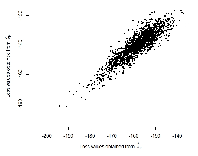
Figure 2: The relationship between the loss values obtained from $\hat{\lambda}_{P}(\mathbold{d,y})$ and $\tilde{\lambda}_{P}(\mathbold{d,y})$ for 100 randomly generated designs under moderate spatial dependence from Example 1

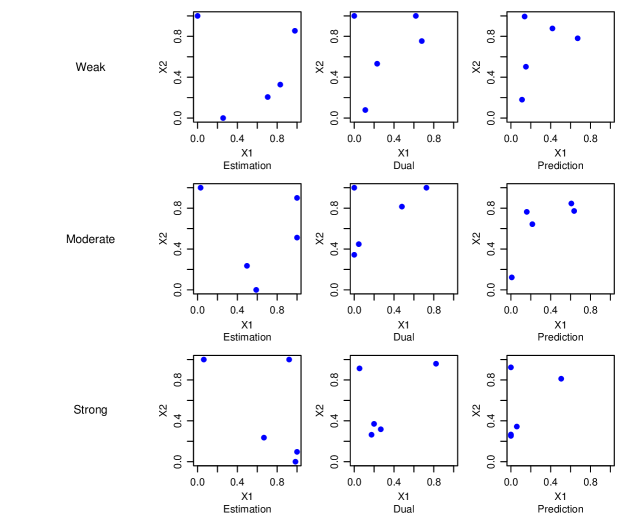
Figure 3: The optimal designs selected from each loss function (n=5)

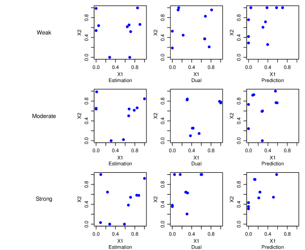
Figure 4: The optimal designs selected from each loss function (n=10)

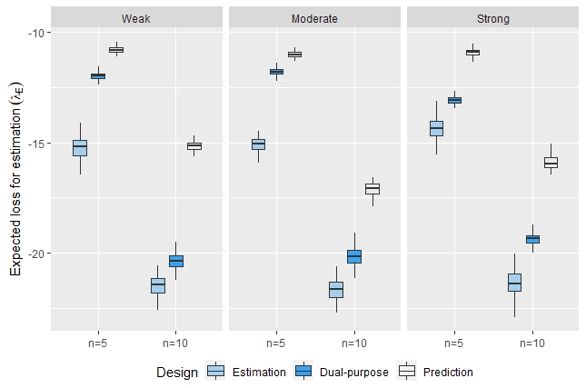
Figure 5: The boxplot of the distribution of the expected values for the loss function that focuses on parameter estimation for different designs over 100 simulations in Example 1

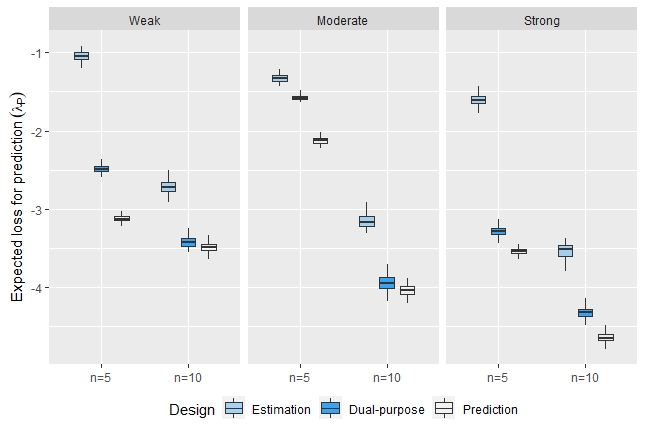
Figure 6: The boxplot of the distribution of the expected values for the loss function that focuses on prediction for different designs over 100 simulations in Example 1

Table 3: Efficiencies of designs selected under each loss function from Example 1

Number of design points	Spatial correlation	Loss function	Estimation efficiency (%)	Prediction efficiency (%)
5	Weak	Estimation	100.00	39.16
		Dual-purpose	78.33	81.15
		Prediction	70.76	100.00
	Moderate	Estimation	100.00	66.75
		Dual-purpose	77.92	81.27
		Prediction	72.96	100.00
	Strong	Estimation	100.00	49.62
		Dual-purpose	91.62	93.47
		Prediction	76.58	100.00
10	Weak	Estimation	100.00	77.72
		Dual-purpose	94.27	97.42
		Prediction	70.21	100.00
	Moderate	Estimation	100.00	78.58
		Dual-purpose	93.43	98.01
		Prediction	78.88	100.00
	Strong	Estimation	100.00	75.61
		Dual-purpose	90.33	92.95
		Prediction	74.65	100.00

6.2  Example 2: Motivating example revisited

Here, we assess the performance of Algorithm 1 and the dual-purpose loss function in finding a retrospective design for Queensland’s air quality monitoring network based on two pollutants $NO_{2}$ and $PM_{2.5}$. Similar to Example 1, $Y_{1}$ ($NO_{2}$) was assumed to follow a Normal distribution while $Y_{2}$ ($PM_{2.5}$) was assumed to follow a Poisson distribution as follows:

$$Y_{1}|s_{1}\sim N(\mu_{1},\sigma^{2})\hskip 14.22636pt\text{and}\hskip 14.22636pt\mu_{1}=\beta_{10}+\beta_{11}X_{1}+\beta_{12}X_{2}+s_{1},$$

$$Y_{2}|s_{2}\sim Pois(\exp(\mu_{2}))\hskip 14.22636pt\text{and}\hskip 14.22636pt\mu_{2}=\beta_{20}+\beta_{21}X_{1}+\beta_{22}X_{3}+s_{2},$$

where $X_{1},X_{2}$ and $X_{3}$ are the Y-coordinate (in UTM system), annual mean humidity level, and the annual mean wind speed measured at the given location, respectively. Again, the Matérn covariance functions with parameters $(\mathbold{\gamma}_{1},\nu_{1})$ and $(\mathbold{\gamma}_{2},\nu_{2})$ were used to form each variance-covariance matrix to capture the spatial variability in each response.

To find the prior distributions for the parameters, we considered the data collected from the sampled locations over the period from 2013 to 2016. First, for each parameter, vague prior distributions were assumed. Then, the observed data were used to update this prior information to obtain a posterior distribution. It is this posterior distribution that was used for design selection as detailed in Algorithm 1. Here, the purpose of this experiment is to select an optimal set of monitoring stations to collect data so that they can be used to predict the annual $NO_{2}$ and $PM_{2.5}$ concentrations for all the monitoring stations in the network. As such, the optimal design is selected from all available locations across the network (i.e. both sampled and unsampled locations).

Results: Similar to the first example, we compared values of loss functions $\tilde{\lambda}_{P}(\mathbold{d,y})$ and $\hat{\lambda}_{P}(\mathbold{d,y})$ for 100 randomly generated designs each with 10 design points. Again, similar loss function values were obtained from each approximation, see Figure 7. As such, adopting our approximation to form efficient designs seems reasonable in this example.

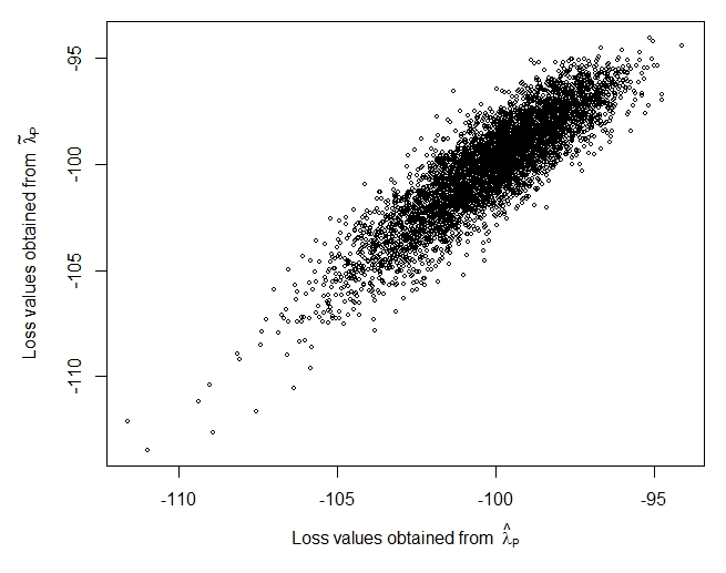
Figure 7: The relationship between the loss values obtained from $\hat{\lambda}_{P}(\mathbold{d,y})$ and $\tilde{\lambda}_{P}(\mathbold{d,y})$ for 100 randomly generated designs from Example 2

In Table 4, we have summarised the designs found for different values of $n$ under each loss function. The numbers shown in this table correspond to the monitoring stations in Figure 1, with the bold numbers representing the sampled locations. Figure 8 shows the locations of the selected monitoring stations under each loss function. It can be seen that the designs selected under each loss function are different but have common stations. Further, when comparing the designs with 5 or 7 design points, it can be seen that the designs points selected from $\lambda_{E}(\mathbold{d,y})$ were spread over the three clusters (C1, C2 and C3) while the majority of design points selected from $\lambda_{P}(\mathbold{d,y})$ and $\lambda_{D}(\mathbold{d,y})$ were clustered in C3. Since a large number of predicted locations belonged to C3, to minimise the prediction uncertainty, it seems reasonable to select more design points from C3 when $\lambda_{P}(\mathbold{d,y})$ and $\lambda_{D}(\mathbold{d,y})$ were responsible for design selection. For the designs with 10 or 15 designs points, the prediction only design points were also spread over the three clusters while the majority of dual-purpose design points were clustered around sampled locations in C2 and C3.

After locating the designs under each loss function, parameter estimation and prediction performance was assessed. Similar to Example 1, we considered 100 independent evaluations of the expected loss under each design objective. Figure 9 shows the distribution of values of the expected loss in terms of parameter estimation under different designs. Similar to Example 1, all estimation designs have lower expected loss when compared to other designs. As in the simulated example, the dual-purpose designs appear to be highly efficient in terms of parameter estimation, and this efficiency appears to increase with $n$. The results also show that the relative performance of the prediction designs decreases as $n$ increases. Figure 10 shows the distribution of expected loss values under the prediction loss function for different designs. As can be seen, the designs selected under the dual-purpose loss function perform well compared to the prediction only designs. Further, the relative performance of the estimation designs for prediction appears to decrease with $n$.

Table 5 shows the design efficiencies in terms of parameter estimation and prediction. Of note, the dual-purpose designs generally maintain high efficiency under both objectives. For designs found under the other two objectives, there are occasions each perform relatively poorly, highlighted by efficiencies of less than 70%.

Table 4: The optimal monitoring stations selected under each loss function

$n$	Estimation design	Dual-purpose design	Prediction design
5	15,21,27,31,33	8,11,14,31,33	2,11,21,25,31
7	2,12,25,27,28,29,34	5,8,11,21,27,33,35	5,11,14,21,26,29,34
10	5,6,8,9,11,14,15,28,29,31	2,5,8,11,21,24,25,26,27,33	5,6,8,11,21,24,27,33,34,35
15	1,2,3,5,6,8,9,11,14,15,	2,5,8,9,11,14,15,21,27,28,	2,3,6,14,15,21,24,25,27,28,
	28,29,31,34,35	29,31,33,34,35	29,31,33,34,35

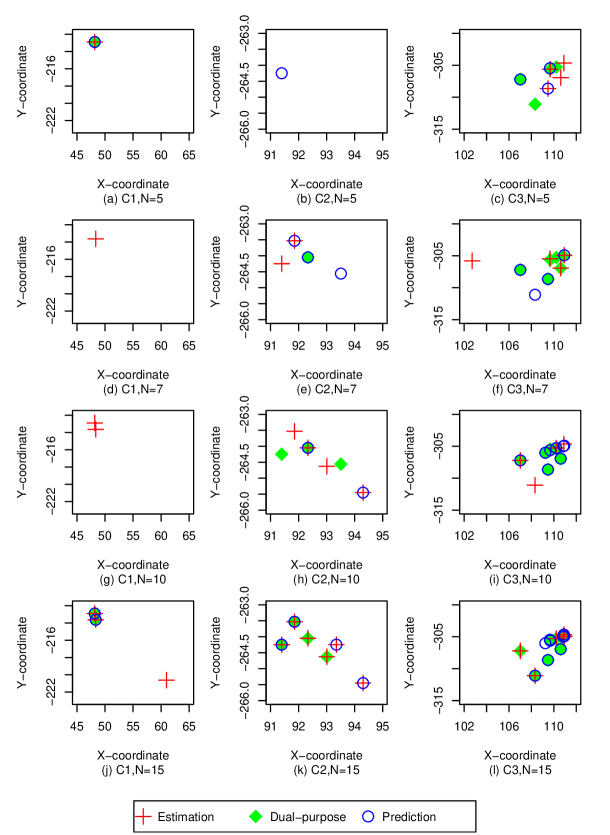
Figure 8: The optimal monitoring stations selected from each loss function

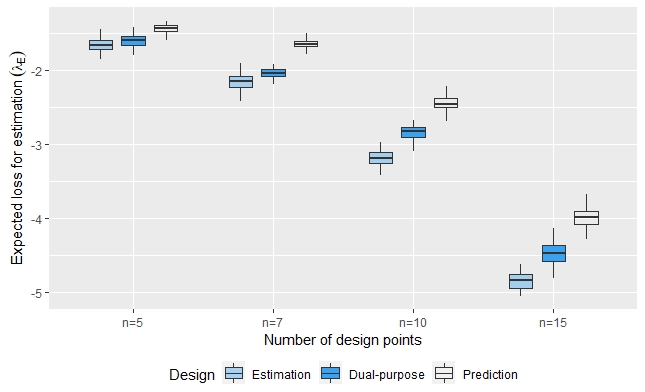
Figure 9: The boxplot of the distribution of the expected values for the loss function that focuses on parameter estimation for different designs over 50 simulations in Example 2

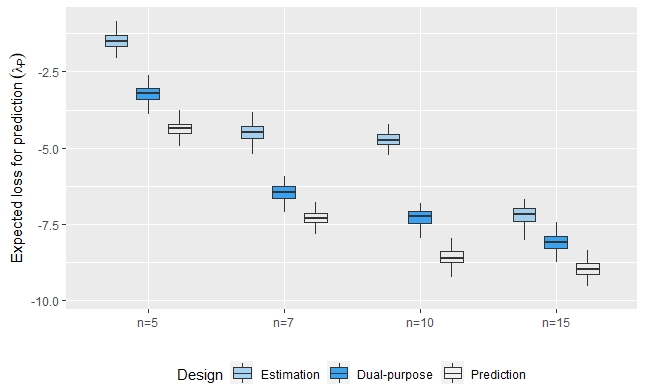
Figure 10: The boxplot of the distribution of the expected values for the loss function that focuses on prediction for different designs over 50 simulations in Example 2

Table 5: Efficiencies of designs selected under each loss function from Example 2

Number of design points	Loss function	Estimation efficiency (%)	Prediction efficiency (%)
5	Estimation	100.00	34.69
	Dual-purpose	96.56	74.91
	Prediction	85.11	100.00
7	Estimation	100.00	61.57
	Dual-purpose	95.16	89.47
	Prediction	75.99	100.00
10	Estimation	100.00	55.58
	Dual-purpose	89.1	85.44
	Prediction	76.01	100.00
15	Estimation	100.00	79.61
	Dual-purpose	91.94	89.76
	Prediction	82.46	100.00

To further investigate future designs for monitoring air quality in Queensland, we re-ran this example by only considering the monitoring stations in C3. Optimal designs with 5 and 7 design points were selected using the three loss functions with the same prior distribution as detailed at the beginning of this example. The selected optimal designs are shown in Figure 11 in the Appendix A. Similar to the above results, the dual-purpose designs remain highly efficient for both design objectives (see Table 6). Further, the relative performance of the single purpose designs appear to decrease as $n$ increases, see Figures 12 and 13.

7  Discussion

In this paper, we have developed a Bayesian design approach to minimise uncertainty in spatial predictions. The approach is based on the derivation of a dual-purpose loss function which quantifies the uncertainty in a given spatial process. Given the substantial computational time needed to evaluate this loss function, a number of approximations were proposed, and these were shown to work well for locating an optimal design. In addition, we extended our methodology to handle bivariate responses in spatial settings, and this was motivated by what has been observed in real-world studies.

In the first example, three design scenarios were considered to test our proposed algorithm and the dual-purpose loss function under various levels of spatial dependence. Overall, the results showed that the dual-purpose designs remained highly efficient under each objective, and this was despite some single objective designs being inefficient under the other objective. Similar results were observed when designing Queensland’s air quality monitoring network based on two air quality measurements $NO_{2}$ and $PM_{2.5}$. The clustered nature of the stations (in terms of spatial locations) was accounted for via the range parameter in our covariance function which resulted in the three clusters being independent. Alternative approaches and/or covariance functions to account for this clustering could be considered in the future, and this may have implications in terms of the design.

Despite the theoretical underpinnings of the loss functions developed in this study, the computational complexity of the loss function $\lambda_{P}(\mathbold{d,y})$ is a drawback of this design approach. Indeed, this difficulty led to the development of an efficient approximation based on the joint distribution of the parameters and the data. We evaluated the proposed approximation to the loss functions, in terms of the accuracy and the computational time required to obtain the approximate loss values. A comparison of the computational times required to evaluate each approximation is shown in Figures 14 and 15. This was based on evaluating 500 independent utilities on a computer with an Intel core-i7 processor running at 2.2 Gigahertz. For the models considered in this paper, this was shown to yield a reasonable approximation. However, such an approach may not be appropriate in general. For example, if bivariate continuous and binary data were observed, it is unlikely that a Multivariate Normal approximation will be appropriate for estimating the entropy of the distribution of the data. As such, alternative methods are needed, and this is an area we plan to explore into the future.

Another possible extension to this work could include quantifying the uncertainty in different components of the spatial process. This can be achieved by quantifying the uncertainty in the mean model and the covariance function, potentially following the work of Borth (1975); McGree (2017). The proposed loss function could then consider a set of all plausible mean and covariance functions, which is flexible enough to represent the uncertainty in the spatial process (Pilz et al., 1997). In studies where high-dimensional multivariate data are observed, it may be necessary to adopt particular Vine-Copulas (Brechmann et al., 2013; Panagiotelis et al., 2017). Other areas we hope to pursue into the future include extensions to quantify uncertainty in temporal (and thus, spatio-temporal) processes (Liu and Vanhatalo, 2019).

Appendix A

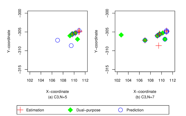
Figure 11: The optimal monitoring stations selected from C3 in Example 2 using each loss function

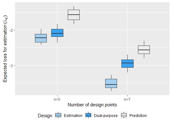
Figure 12: The boxplot of the distribution of the expected values for the loss function that focuses on parameter estimation for different designs over 50 simulations from C3 in Example 2

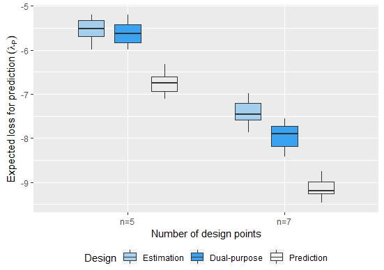
Figure 13: The boxplot of the distribution of the expected values for the loss function that focuses on prediction for different designs over 50 simulations from C3 in Example 2

Table 6: Efficiencies of designs selected under each loss function from C3 in Example 2

Number of design points	Loss function	Estimation efficiency (%)	Prediction efficiency (%)
5	Estimation	100.00	80.62
	Dual-purpose	93.56	82.88
	Prediction	71.73	100.00
7	Estimation	100.00	82.03
	Dual-purpose	83.13	87.34
	Prediction	72.13	100.00

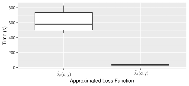
Figure 14: The comparison of computational time required to estimate the two loss functions for Example 1

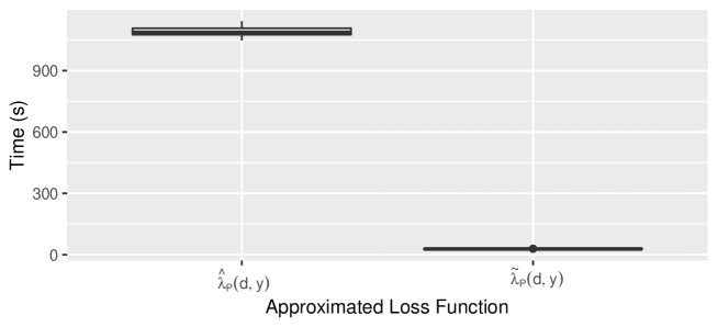
Figure 15: The comparison of computational time required to estimate the two loss functions for Example 2

Appendix B

In spatial settings, the literature suggests that parameter estimation designs often feature clustered sampling points (Diggle and Ribeiro, 2007). Here the ratio of the range and nugget to the partial sill influence the configuration of clusters. In contrast, the prediction designs often resemble a regularly spaced design. It is presumed that designs for both of these goals will combine features from both.

In Example 1, we potentially observe some of the above features across the three different designs with some apparent difference. To investigate about these differences, a new simulation study has been conducted where the estimation and prediction performance of a selected set of designs were evaluated. These designs were: an equally spaced triangular design, a design with all the points on the boundary, and a design with all points close to the prediction locations, see Figure 16 below which shows these three designs. The performance of these designs for estimation and prediction were compared to the designs found in this work.

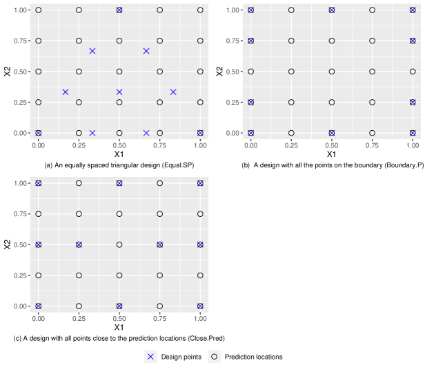
Figure 16: A selected set of theoretical designs

To evaluate the prediction performance of the designs shown in Figure 16, we evaluated the expected prior and posterior prediction variance at each of the prediction locations. This was achieved by simulating 500 data sets from each design and approximating the posterior distribution for each. For each of these posterior distributions, posterior predictive data were simulated at each prediction location, and then the variance of these at each location was evaluated. The average of this variance was then evaluated across the 500 simulations. The results for this for both responses are shown in Figures 17 and 18.

From Figure 17, it is clear that the prediction design found in our paper yields the smallest average prediction variance across all locations. The next best design appears to be the ‘close.pred’ design suggesting that a design that is more regularly spaced across the entire region performs well here for prediction, and this is what would be expected based on results from the literature. Otherwise, there appears to be very little difference in the performance of the remaining designs. Given one of these designs in the estimation design found in our work, then potentially these designs are focussing more on estimation.

From Figure 18, similar conclusions can be drawn.

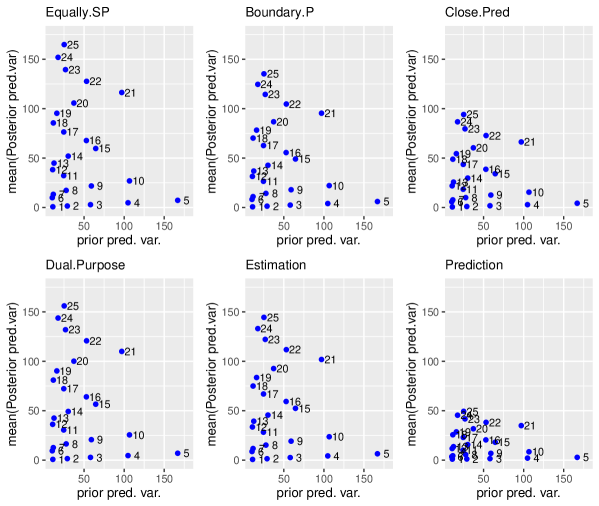
Figure 17: Posterior prediction variances vs prior prediction variances of response 1 (Y1) for prediction locations

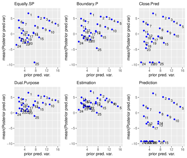
Figure 18: Posterior prediction variances vs prior prediction variances of response 2 (Y2) for prediction locations

To evaluate the estimation performance of the designs, a similar approach to evaluate the prediction performance was followed. That is, 500 prior predictive data sets were generated based on each design, and a posterior distribution was found for each. The average posterior variance of each parameter was then evaluated based on each design. These averages are shown in Figure 19. Across all designs, there does not appear to be an appreciable difference in terms of estimation performance. However, our estimation design is performing better but only marginally. This may be because the prior variance for most parameters is quite low, so attention may be given to estimating $\beta_{11},\beta_{12}$ and $\beta_{10}$ more precisely. To do so, at least for the slope terms, a contrast between data collected at extreme values of X1 and also X2 would seem useful, and this is a feature of all designs considered.

The above highlights the potentially influence the prior distribution can have in Bayesian design, and provide a potential reason for differences observed between our designs and those that might be considered as being more standard for estimation and prediction in spatial settings. Given this, such standard designs may not necessarily be optimal under a variety of prior configurations. This was observed here but we also note that these standard designs did not perform poorly.

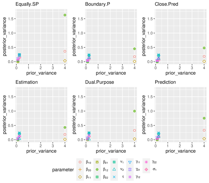
Figure 19: The prior variance vs the posterior variance for each parameter for different designs

References

- (1)
- Albert and McShane (1995) Albert, P. S. and McShane, L. M. (1995), ‘A generalized estimating equations approach for spatially correlated binary data: Applications to the analysis of neuroimaging data’, Biometrics 51(2), 627–638.
- Bárdossy (2006) Bárdossy, A. (2006), ‘Copula-based geostatistical models for groundwater quality parameters’, Water Resources Research 42(11).
- Bloom and Kentwell (1999) Bloom, L. M. and Kentwell, D. J. (1999), A geostatistical analysis of cropped and uncropped soil from the jimperding brook catchment of western australia, in J. Gómez-Hernández, A. Soares and R. Froidevaux, eds, ‘geoENV II — Geostatistics for Environmental Applications’, Springer Netherlands, Dordrecht, pp. 369–379.
- Bohorquez et al. (2017) Bohorquez, M., Giraldo, R. and Mateu, J. (2017), ‘Multivariate functional random fields: prediction and optimal sampling’, Stochastic Environmental Research and Risk Assessment 31(1), 53–70.
- Borth (1975) Borth, D. M. (1975), ‘A total entropy criterion for the dual problem of model discrimination and parameter estimation’, Journal of the Royal Statistical Society. Series B (Methodological) pp. 77–87.
- Brechmann et al. (2013) Brechmann, E. C., Schepsmeier, U. et al. (2013), ‘Modeling dependence with C-and D-vine Copulas: The R-package CDVine’, Journal of Statistical Software 52(3), 1–27.
- Bruno et al. (2001) Bruno, R., Palumbo, V. and Bonduà, S. (2001), Identification of regional variability component by geostatistical analysis of stream sediments, in P. Monestiez, D. Allard and R. Froidevaux, eds, ‘geoENV III — Geostatistics for Environmental Applications’, Springer Netherlands, Dordrecht, pp. 113–123.
- Castrignanò et al. (2008) Castrignanò, A., Buttafuoco, G. and Giasi, C. (2008), Assessment of groundwater salinisation risk using multivariate geostatistics, in A. Soares, M. J. Pereira and R. Dimitrakopoulos, eds, ‘geoENV VI – Geostatistics for Environmental Applications: Proceedings of the Sixth European Conference on Geostatistics for Environmental Applications’, Springer Netherlands, Dordrecht, pp. 191–202.
- Clayton (1978) Clayton, D. G. (1978), ‘A model for association in bivariate life tables and its application in epidemiological studies of familial tendency in chronic disease incidence’, Biometrika 65(1), 141–151.
- Cook and Johnson (1981) Cook, R. D. and Johnson, M. E. (1981), ‘A family of distributions for modelling non-elliptically symmetric multivariate data’, Journal of the Royal Statistical Society. Series B (Methodological) 43(2), 210–218.
- Cook and Wong (1994) Cook, R. D. and Wong, W. K. (1994), ‘On the equivalence of constrained and compound optimal designs’, Journal of the American Statistical Association 89(426), 687–692.
- Diggle and Lophaven (2006) Diggle, P. and Lophaven, S. (2006), ‘Bayesian geostatistical design’, Scandinavian Journal of Statistics 33(1), 53–64.
- Diggle and Ribeiro (2007) Diggle, P. and Ribeiro, P. J. (2007), Model-based Geostatistics, Springer Series in Statistics, Springer, New York.
- Diggle et al. (2003) Diggle, P., Ribeiro, P. J. and Christensen, O. F. (2003), An introduction to model-based geostatistics, in J. Møller, ed., ‘Spatial Statistics and Computational Methods’, Springer New York, pp. 43–86.
- Durante and Sempi (2010) Durante, F. and Sempi, C. (2010), Copula theory: an introduction, in ‘Copula theory and its applications’, Springer, pp. 3–31.
- Falk et al. (2014) Falk, M. G., McGree, J. M. and Pettitt, A. N. (2014), ‘Sampling designs on stream networks using the pseudo-Bayesian approach’, Environmental and Ecological Statistics 21(4), 751–773.
- Fuentes et al. (2007) Fuentes, M., Chaudhuri, A. and Holland, D. M. (2007), ‘Bayesian entropy for spatial sampling design of environmental data’, Environmental and Ecological Statistics 14(3), 323–340.
- Genest and MacKay (1986) Genest, C. and MacKay, J. (1986), ‘The joy of Copulas: bivariate distributions with uniform marginals’, The American Statistician 40(4), 280–283.
- Gómez-Rubio et al. (2019) Gómez-Rubio, V., Bivand, R. S. and Rue, H. (2019), Spatial models using laplace approximation methods, in M. M. Fischer and P. Nijkamp, eds, ‘Handbook of Regional Science’, Springer, Berlin, Heidelberg, pp. 1–16.
- Gräler and Pebesma (2011) Gräler, B. and Pebesma, E. (2011), ‘The pair-Copula construction for spatial data: a new approach to model spatial dependency’, Procedia Environmental Sciences 7, 206 – 211.
- Hill et al. (1968) Hill, W. J., Hunter, W. G. and Wichern, D. W. (1968), ‘A joint design criterion for the dual problem of model discrimination and parameter estimation’, Technometrics 10(1), 145–160.
- Huang et al. (2019) Huang, Y., Hanneke, R. and Jones, R. (2019), ‘Bibliometric analysis of cardiometabolic disorders studies involving , and noise exposure’, BMC Public Health 19(1), 1–14.
- Jiang et al. (2016) Jiang, X. Q., Mei, X. D. and Feng, D. (2016), ‘Air pollution and chronic airway diseases: what should people know and do?’, Journal of thoracic disease 8(1), 31–40.
- Joe (2014) Joe, H. (2014), Dependence Modeling with Copulas, 1 edn, New York: Chapman and Hall/CRC.
- Kazianka and Pilz (2011) Kazianka, H. and Pilz, J. (2011), ‘Bayesian spatial modeling and interpolation using Copulas’, Computers & Geosciences 37(3), 310 – 319.
- Kullback and Leibler (1951) Kullback, S. and Leibler, R. A. (1951), ‘On information and sufficiency’, The Annals of Mathematical Statistics 22(1), 79–86.
- Le et al. (2003) Le, N. D., Sun, L. and Zidek, J. V. (2003), Designing networks for monitoring multivariate environmental fields using data with monotone pattern, Technical report, TR 2003-5, Statistical and Applied Mathematical Sciences Institute, RTP, NC.
- Le and Zidek (2006) Le, N. D. and Zidek, J. V. (2006), Statistical analysis of environmental space-time processes, in ‘Springer Series in Statistics’, Springer, New York, NY.
- Liu and Vanhatalo (2019) Liu, J. and Vanhatalo, J. (2019), ‘Bayesian model based spatiotemporal survey designs and partially observed log Gaussian cox process’, Spatial Statistics 35, 1–27.
- Long et al. (2013) Long, Q., Scavino, M., Tempone, R. and Wang, S. (2013), ‘Fast estimation of expected information gains for Bayesian experimental designs based on Laplace approximations’, Computer Methods in Applied Mechanics and Engineering 259, 24 – 39.
- McGree (2017) McGree, J. M. (2017), ‘Developments of the total entropy utility function for the dual purpose of model discrimination and parameter estimation in Bayesian design’, Computational Statistics and Data Analysis 113, 207–225.
- McGree et al. (2008) McGree, J. M., Eccleston, J. A. and Duffull, S. B. (2008), ‘Compound optimal design criteria for nonlinear models’, Journal of Biopharmaceutical Statistics 18(4), 646–661.
- Meyer and Nachtsheim (1995) Meyer, R. K. and Nachtsheim, C. J. (1995), ‘The coordinate-exchange algorithm for constructing exact optimal experimental designs’, Technometrics 37(1), 60–69.
- Müller et al. (2004) Müller, P., Sansó, B. and Iorio, M. D. (2004), ‘Optimal bayesian design by inhomogeneous Markov chain simulation’, Journal of the American Statistical Association 99(467), 788–798.
- Müller (2007) Müller, W. (2007), Collecting Spatial Data, 3rd revised and extended edition, Springer Verlag, Heidelberg.
- Musafer and Thompson (2017) Musafer, G. N. and Thompson, M. H. (2017), ‘Non-linear optimal multivariate spatial design using spatial vine Copulas’, Stochastic Environmental Research and Risk Assessment 31(2), 551–570.
- Nelsen (2006) Nelsen, R. (2006), ‘An introduction to Copulas, 2nd’, New York: SpringerScience Business Media .
- Overstall, McGree and Drovandi (2018) Overstall, A. M., McGree, J. M. and Drovandi, C. C. (2018), ‘An approach for finding fully Bayesian optimal designs using normal-based approximations to loss functions’, Statistics and Computing 28(2), 343–358.
- Overstall and Woods (2017) Overstall, A. M. and Woods, D. C. (2017), ‘Bayesian design of experiments using approximate coordinate exchange’, Technometrics 59(4), 458–470.
- Overstall, Woods and Adamou (2018) Overstall, A. M., Woods, D. C. and Adamou, M. (2018), ‘acebayes: An R package for Bayesian optimal design of experiments via approximate coordinate exchange’, arXiv:1705.08096 .
- Panagiotelis et al. (2017) Panagiotelis, A., Czado, C., Joe, H. and Stöber, J. (2017), ‘Model selection for discrete regular vine Copulas’, Computational Statistics & Data Analysis 106, 138–152.
- Pilz et al. (1997) Pilz, J., Schimek, M. and Spöck, G. (1997), Taking account of uncertainty in spatial covariance estimation, in ‘Geostatistics Wollongong 96’, Vol. 8, Kluwer Academic, pp. 302–313.
- Roberts et al. (2019) Roberts, S., Arseneault, L., Barratt, B., Beevers, S., Danese, A., Odgers, C. L., Moffitt, T. E., Reuben, A., Kelly, F. J. and Fisher, H. L. (2019), ‘Exploration of and air pollution and mental health problems using high-resolution data in london-based children from a uk longitudinal cohort study’, Psychiatry Research 272, 8–17.
- Tao et al. (2013) Tao, Y., Liu, J., Li, Z., Lin, J., Lu, T. and Yan, F. (2013), ‘Dose-finding based on bivariate efficacy-toxicity outcome using archimedean Copula’, PLoS ONE 8(11), 1–6.
- Watson (2006) Watson, K. E. (2006), ‘Air pollution and heart disease’, Reviews in cardiovascular medicine 7(1), 44–44.
- Zhang et al. (2016) Zhang, S., Li, G., Tian, L., Guo, Q. and Pan, X. (2016), ‘Short-term exposure to air pollution and morbidity of copd and asthma in east asian area: A systematic review and meta-analysis’, Environmental research 148, 15–23.