Substitution of subspace collections with nonorthogonal subspaces to accelerate Fast Fourier Transform methods applied to conducting composites

Abstract

We show the power of the algebra of subspace collections developed in Chapter 7 of [24]. Specifically we accelerate the Fast Fourier Transform schemes of Moulinec and Suquet ([27], [28]) and [7], for computing the fields and effective tensor in a conducting periodic medium by substituting a subspace collection with nonorthogonal subspaces inside one with orthogonal subspaces. This can be done when the effective conductivity as a function of the conductivity $\sigma_{1}$ of the inclusion phase (with the matrix phase conductivity set to $1$) has its singularities confined to an interval $[-\beta,-\alpha]$ of the negative real $\sigma_{1}$ axis. Numerical results of Moulinec and Suquet show accelerated convergence for the model example of a square array of squares at $25\%$ volume fraction. For other problems we show how $Q^{*}_{C}$-convex functions can be used to restrict the region where singularities of the effective tensor as a function of the component tensors might be found.

1 Introduction

Subspace collections with orthogonal subspaces obviously have a lot of relevance to physical problems. Here we give an example to show that subspace collections with nonorthogonal subspaces are an important tool in analysis, reaching beyond their connection with rational functions of several complex variables. This chapter is mostly self-contained. While it uses nonorthogonal subspace collections, it is not necessary for the reader to have read Chapter 7 of [24]. However, it is recommended for the reader to look at Chapters 1 and 2 in that book.

The specific problem we consider is a two-component conducting medium with conductivities $\sigma_{1}$ and $\sigma_{2}$, phase $1$ being the inclusion phase. The dimension is $d=2$ or $d=3$. Without loss of generality we can take $\sigma_{2}=1$. Assume for simplicity that the composite has square $(d=2)$ or cubic $(d=3)$ symmetry so that the effective conductivity tensor is isotropic, taking the form $\sigma_{*}{\bf I}$. [2] made the pioneering observation that the function $\sigma_{*}(\sigma_{1})$ is an analytic function of $\sigma_{1}$ and has all its singularities on the negative real axis. He made some assumptions which were not valid [17]. These assumptions could be circumvented by approximating the composite by a large resistor network ([18]). Subsequently Golden and Papanicolaou ([9], [10]) gave a rigorous proof of the analytic properties. Here we make the additional assumption (only true for some geometries) that the function $\sigma_{*}(\sigma_{1})$ has all its singularities confined to an interval $[-\beta,-\alpha]$ on the negative real axis, $\alpha>0$ and $\beta>\alpha$ (see 1). This information results in tighter bounds on the conductivity and complex conductivity, or equivalently the complex dielectric constant, ([4]; [35]; [8]), and these bounds may be inverted to yield information about $\alpha$ and $\beta$ from experimental measurements ([31]). By contrast, here our goal is to utilize the information to improve the speed of convergence of Fast Fourier Transform methods for computing the fields in composites and their associated effective tensors. These methods were first introduced by Moulinec and Suquet ([27], [28]): see [26] for a recent review. One important application has been to viscoplastic polycrystals ([14], [15]). For materials with a linear response, previous significant advances in the acceleration of these schemes were made by [7] (see also the generalization in section 14.9 of [21], and in particular equation (14.38)), and by [39] and [38].

Figure 1: We assume that in the complex $\sigma_{1}$-plane, the function $\sigma_{*}(\sigma_{1})$ has all its singularities on the negative real $\sigma_{1}$-axis, between $\sigma_{1}=-\alpha$ and $\sigma_{1}=-\beta$. Here the zig-zag line denotes a possible branch cut.

The singularities in the interval $[-\beta,-\alpha]$ could be poles or could be a branch cut (if the inclusion has sharp corners, or if there is some randomness in the geometry). Note it is not only the effective conductivity which has this analytic form but also the electric field ${\bf E}({\bf x},\sigma_{1})$ and current field ${\bf J}({\bf x},\sigma_{1})$ at fixed ${\bf x}$, and fixed applied field, with $\sigma_{1}$ varying. If we didn’t know anything about $\alpha$ and $\beta$ there could potentially be singularities anywhere along the negative real $\sigma_{1}$ axis. Let’s first look at the case $\alpha=0$, $\beta=\infty$.

The original Fast Fourier Transform scheme of Moulinec and Suquet ([27], [28]) is based on series expansions, such as (2.35) in [24], which for conductivity takes the form

$$\mbox{\boldmath${\sigma}$}_{*}=\sigma_{0}{\bf I}+\sum_{j=0}^{\infty}\mbox{\boldmath${\Gamma}$}_{0}[\mbox{\boldmath${\sigma}$}({\bf x})-\sigma_{0}{\bf I}][\mbox{\boldmath${\Gamma}$}_{1}({\bf I}-\mbox{\boldmath${\sigma}$}/\sigma_{0})]^{j}\mbox{\boldmath${\Gamma}$}_{0},\quad{\bf e}={\bf e}_{0}+\sum_{j=0}^{\infty}[\mbox{\boldmath${\Gamma}$}_{1}({\bf I}-\mbox{\boldmath${\sigma}$}/\sigma_{0})]^{j}{\bf e}_{0},$$ (1.1)

for the effective conductivity $\mbox{\boldmath${\sigma}$}_{*}$, and electric field ${\bf e}({\bf x})$, with ${\bf e}_{0}$ being the applied (average) electric field. [To obtain (1.1) from (2.35) in [24] we use the fact that $\mbox{\boldmath${\Gamma}$}_{0}(\sigma_{0}{\bf I})\mbox{\boldmath${\Gamma}$}_{1}=0$.] Their key and beautiful idea was that since the action of $\mbox{\boldmath${\Gamma}$}_{1}$ is readily evaluated in Fourier space, while the action of $({\bf I}-\mbox{\boldmath${\sigma}$}/\sigma_{0})$ is readily evaluated in real space, both $\mbox{\boldmath${\sigma}$}_{*}$ and ${\bf e}({\bf x})$ can be readily calculated from these series by going back and forth between real and Fourier space, using Fast Fourier Transforms to do so.

In a two-phase medium with isotropic conductivities $\sigma_{1}$ and $\sigma_{2}=1$, and with the choice of $\sigma_{0}=\frac{1}{2}(\sigma_{1}+\sigma_{2})=\frac{1}{2}(\sigma_{1}+1)$ used by Moulinec and Suquet, $({\bf I}-\mbox{\boldmath${\sigma}$}/\sigma_{0})$ takes the value $(1-\sigma_{1})/(\sigma_{1}+1)$ in phase 1 and the value $-(1-\sigma_{1})/(\sigma_{1}+1)$ in phase 2. So it is clear that this scheme gives an expansion of the form

$$\sigma_{*}/\sigma_{0}=1+\sum_{n=1}^{\infty}a_{n}\left(\frac{\sigma_{1}-1}{\sigma_{1}+1}\right)^{n}.$$ (1.2)

The transformation $z=(\sigma_{1}-1)/(\sigma_{1}+1)$ maps the right half of the complex plane to the unit disk (see 2).

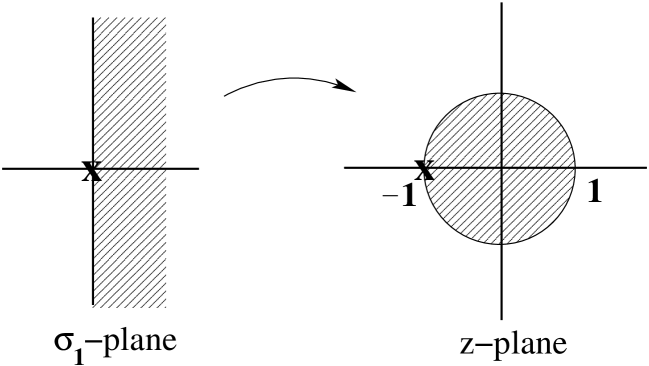
Figure 2: If we want a series expansion which converges in the entire right half of the $\sigma_{1}$-plane, when a singularity is located at the point ${\bf X}$, then we make a fractional linear transformation which takes the right half of the $\sigma_{1}$-plane to the unit disk in the $z$-plane, and find an series expansion in powers of $z$. The scheme of Moulinec and Suquet ([27], [28]) provides such an expansion.

So with $\alpha=0$ the series will converge if $|z|<1$, i.e., in the entire right half of the complex $\sigma_{1}-$plane, $\mathop{\rm Re}\nolimits(\sigma_{1})>0$. (Recall that it is the distance from the origin to the nearest singularity in the $z-$plane which determines the radius of convergence in the $z-$plane, and hence the region of convergence in the $\sigma_{1}-$plane.)

With the accelerated scheme of [7] (see also the generalization in section 14.9 of [21], and in particular equation (14.38)), one has the expansion

$$\sigma_{*}/\sqrt{\sigma_{1}}=1+\sum_{n=1}^{\infty}b_{n}\left(\frac{\sqrt{\sigma_{1}}-1}{\sqrt{\sigma_{1}}+1}\right)^{n}.$$ (1.3)

The transformation $z=(w-1)/(w+1)$ where $w=\sqrt{\sigma_{1}}$ maps the $\sigma_{1}$ complex plane minus the slit along the negative real axis to the unit disk $|z|=1$ (see 3).

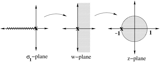
Figure 3: If we want a series expansion which converges in the entire the $\sigma_{1}$-plane minus the negative real $\sigma_{1}$-axis, then we first make a square root transformation which maps the cut complex $\sigma_{1}$-plane to the right half of the $w$-plane, followed by a fractional linear transformation which takes it to the unit disk in the $z$-plane, and find an expansion in powers of $z$. The scheme of [7] provides such an expansion.

So with $\alpha=0$ the series will converge if $|z|<1$, i.e., in the entire complex plane minus the slit along the negative real axis. These arguments show that when $\alpha=0$ the accelerated scheme should have a larger region of convergence, and by the same line of reasoning a faster rate of convergence when both schemes converge. (Note, however, that if $\alpha>0$ and $\beta<\infty$ the scheme of Moulinec and Suquet could outperform that of Eyre and Milton for small and very large values of $\sigma_{1}$, since the scheme of Moulinec and Suquet should then converge for sufficiently small or sufficiently large negative real values of $\sigma_{1}$.)

If we know $\alpha$ and $\beta$ (or bounds for them) then it makes sense to use a transformation which maps the complex plane minus the slit $[-\beta,-\alpha]$ to the unit circle $|z|=1$. Since the transformation

$$t=\frac{(\sigma_{1}+\alpha)(1+\beta)}{(\sigma_{1}+\beta)(1+\alpha)}=1+\frac{(\sigma_{1}-1)(\beta-\alpha)}{(\sigma_{1}+\beta)(1+\alpha)}$$ (1.4)

maps the interval $[-\beta,-\alpha]$ to $[-\infty,0]$ and takes $\sigma_{1}=1$ to $t=1$, it is clear that the transformation

$$z=\frac{\sqrt{t}-1}{\sqrt{t}+1}\quad\text{(with $t$ given above)}$$ (1.5)

maps the complex $\sigma_{1}$ plane minus the slit $[-\beta,-\alpha]$ to the unit disk $|z|=1$ (see 4).

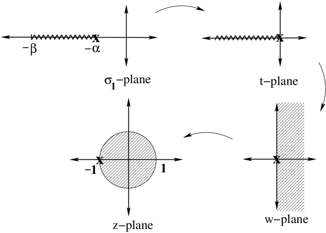
Figure 4: If we want a series expansion which converges in the entire the $\sigma_{1}$-plane minus the cut on $\sigma_{1}$-axis between $-\beta$ and $-\alpha$ then we first use a fractional linear transformation which maps this cut to the entire negative real axis in the $t$-plane, followed by a square root transformation mapping the cut complex $t$-plane to the right half of the $w$-plane, followed by a fractional linear transformation which takes it to the unit disk in the $z$-plane, and find an expansion in powers of $z$. The scheme developed in this chapter provides such an expansion.

So we want to get a Fast Fourier Transform (FFT) method associated with an expansion

$$\frac{\sigma_{*}}{\sqrt{[(\sigma_{1}+\alpha)(1+\beta)]/[(\sigma_{1}+\beta)(1+\alpha)]}}=1+\sum_{n=1}^{\infty}c_{n}\left(\frac{\sqrt{\frac{(\sigma_{1}+\alpha)(1+\beta)}{(\sigma_{1}+\beta)(1+\alpha)}}-1}{\sqrt{\frac{(\sigma_{1}+\alpha)(1+\beta)}{(\sigma_{1}+\beta)(1+\alpha)}}+1}\right)^{n}.$$ (1.6)

It looks rather formidable but really it is just a matter of substituting

$$t=\frac{(\sigma_{1}+\alpha)(1+\beta)}{(\sigma_{1}+\beta)(1+\alpha)}$$ (1.7)

in the [7] scheme associated with

$$\sigma_{*}/\sqrt{t}=1+\sum_{n=1}^{\infty}c_{n}\left(\frac{\sqrt{t}-1}{\sqrt{t}+1}\right)^{n}.$$ (1.8)

But of course one wants to do this substitution at the level of the underlying Hilbert space, not just in the conductivity function.

2 Substitution at the level of the Hilbert space

Substitution at the level of the Hilbert space requires the substitution of subspace collections where the subspaces do not satisfy the orthogonality property. At a discrete level it is easy to get an idea of how this can be done. If we consider the composite as a resistor network, in phase $1$ with resistors having resistance $R_{1}=\delta/\sigma_{1}$, while in phase $2$ with resistors having resistance $R_{2}=\delta/\sigma_{2}$, so e.g., the composite is replaced by a network (see 5(a)).

Figure 5: A composite containing two phases, as for example a periodic array of disks with a unit cell as shown in (a), can be approximated by a discrete network of resistors having resistors $R_{2}$ and $R_{1}$. At this discrete level we are free to replace each resistor having resistance $R_{1}$ by the combination of resistors in figure (b). This transformation at the Hilbert-space level, corresponds to a fractional linear transformation in the $\sigma_{1}$-plane.

Then at this level we could replace each resistor $R_{1}$ by the compound resistor (see 5(b)) with $k_{1},k_{2},k_{3}$ real constants. That is the resistance $R_{1}=\delta/\sigma_{1}$ gets replaced by

$$k_{1}R_{2}+\frac{1}{1/(k_{2}R_{1})+1/(k_{3}R_{2})} = \frac{k_{1}}{\sigma_{2}}+\frac{1}{\sigma_{1}/k_{2}+\sigma_{2}/k_{3}}$$ (2.1)

$$= \frac{k_{1}\sigma_{1}/k_{2}+k_{1}/k_{3}+1}{\sigma_{1}/k_{2}+1/k_{3}},$$

when $\sigma_{2}=1$, and so $\sigma_{1}$ gets replaced by

$$\frac{(\sigma_{1}/k_{2}+1/k_{3})\delta}{k_{1}\sigma_{1}/k_{2}+k_{1}/k_{3}+1},$$ (2.2)

which is a fractional linear transformation of $\sigma_{1}$. In other words, in phase $1$ the number of fields is multiplied by $3$ (replacing one resistor by $3$). Note that with real positive values of $k_{1}$, $k_{2}$ and $k_{3}$ the transformation (2.2) maps the nonnegative real $\sigma_{1}$-axis onto an interval on the positive real axis, and the negative real $\sigma_{1}$-axis onto its complement, which cannot be the desired interval $[-\beta,-\alpha]$. Essentially, instead of making a transformation which has the effect of lengthening the branch cut as desired in the map at the top of 4, we have a transformation which presumably (in some suitably defined metric) shortens the branch cut. This is why it is necessary to substitute nonorthogonal subspace collections, rather than orthogonal ones [see also the discussion below (4.17)], since, as we will see, they only act to lengthen the branch cut.

How to do this in general in the continuum case is described in section 29.1 of [21], bottom of page 621 and page 622, for orthogonal subspace collections, and in the second half of Section 7.8 of [24], without assuming orthogonality. That is a bit abstract so let us go through it for the case in question.

3 The original subspace collection

Our starting point is the Hilbert space ${\cal H}$ of fields ${\bf P}({\bf x})$ (real or complex $d-$dimensional vector fields), that are cell-periodic and square-integrable in the unit cell. We denote ${\chi}$ as the projection onto all fields which are zero in phase $2$, ${\cal U}$ as the space of constant vector fields, ${\cal E}$ as the space of gradients which derive from periodic potentials (i.e., ${\bf E}\in{\cal E}$ if $\nabla\times{\bf E}=0$ and $\langle{\bf E}\rangle=0$) and ${\cal J}$ as the space of divergence free fields with zero average value (i.e., ${\bf J}\in{\cal J}$ if $\nabla\cdot{\bf J}=0$ and $\langle{\bf J}\rangle=0$). In our Hilbert space the inner product is taken to be

$$({\bf P},\widetilde{{\bf P}})=\int_{\text{unit cell}}\overline{{\bf P}({\bf x})}\cdot\widetilde{{\bf P}}({\bf x}),$$ (3.3)

where the overline denotes complex conjugation. With respect to this inner product the $3$ spaces ${\cal U},{\cal E}$ and ${\cal J}$ are orthogonal. The projection onto ${\cal E}$ we denote by $\mbox{\boldmath${\Gamma}$}_{1}$. In Fourier space

$$\mbox{\boldmath${\Gamma}$}_{1}\widehat{{\bf P}}({\bf k})=\left\{\begin{array}[]{lr}\frac{{\bf k}\otimes{\bf k}}{|{\bf k}|^{2}}\widehat{{\bf P}}({\bf k}),&{\bf k}\neq 0,\\ 0,&{\bf k}=0.\end{array}\right.$$ (3.4)

The field equations are solved once we have found electric fields ${\bf E}({\bf x})$ and current fields ${\bf J}({\bf x})$ such that

$${\bf J}=[(\sigma_{1}-\sigma_{2})\mbox{\boldmath${\chi}$}+\sigma_{2}]{\bf E},\quad{\bf E}\in{\cal U}\oplus{\cal E},\quad{\bf J}\in{\cal U}\oplus{\cal J}.$$ (3.5)

The effective tensor $\sigma_{*}$ is then defined via

$$\mbox{\boldmath${\Gamma}$}_{0}{\bf J}=\sigma_{*}\mbox{\boldmath${\Gamma}$}_{0}{\bf E},$$ (3.6)

where $\mbox{\boldmath${\Gamma}$}_{0}$ is the projection onto ${\cal U}$. We assume the composite is isotropic so that $\sigma_{*}$ is a scalar, although the method is easily generalized to anisotropic materials where the effective conductivity is a second order tensor.

4 The vector subspace collection we substitute into the original subspace collection

Now consider a $3-$dimensional subspace collection ${\cal H}^{\prime}$ consisting of $3$ component vectors ${\bf P}=[P_{1},P_{2},P_{3}]^{T}$ with inner product

$$({\bf P},\widetilde{{\bf P}})=\sum_{i=1}^{3}\overline{P}_{i}\widetilde{P}_{i},$$ (4.7)

where the overline denotes complex conjugation. The projection $\mbox{\boldmath${\chi}$}^{\prime}=p\otimes p$ projects onto the one dimensional space of fields proportional to the unit vector ${\bf p}$ where ${\bf p}=[p_{1},p_{2},p_{3}]^{T}$ and $p_{1},p_{2},p_{3}$ are given constants such that $p_{1}^{2}+p_{2}^{2}+p_{3}^{2}=1$. The $p$’s could be complex but we do not mean $|p_{1}|^{2}+|p_{2}|^{2}+|p_{3}|^{2}=1$. Thus $\mbox{\boldmath${\chi}$}^{\prime}$ is a projection but not an orthogonal projection when the $p$’s are complex, as then $\mbox{\boldmath${\chi}$}^{\prime}=p\otimes p$ is not Hermitian. We take the following:

$${\cal U}^{\prime}\text{ is the space of fields proportional to }(1,0,0)^{T},$$

$${\cal E}^{\prime}\text{ is the space of fields proportional to }(0,1,0)^{T},$$

$${\cal J}^{\prime}\text{ is the space of fields proportional to }(0,0,1)^{T},$$

$${\cal P}_{1}\text{ is the space of fields proportional to }(p_{1},p_{2},p_{3})^{T},$$

$${\cal P}_{2}\text{ is the space of fields }(P_{1},P_{2},P_{3})^{T}$$

$$\text{such that }p_{1}P_{1}+p_{2}P_{2}+p_{3}P_{3}=0.$$ (4.8)

The field equations become

$${\bf J}^{\prime}=[(t-\sigma_{2})\mbox{\boldmath${\chi}$}^{\prime}+\sigma_{2}]{\bf E}^{\prime},\quad{\bf E}^{\prime}\in{\cal U}^{\prime}\oplus{\cal E}^{\prime},\quad{\bf J}^{\prime}\in{\cal U}^{\prime}\oplus{\cal J}^{\prime},$$ (4.9)

where the constant $t$ will be chosen so the associated “effective modulus” is $\sigma_{1}$. That is

$$\mbox{\boldmath${\Gamma}$}_{0}{\bf J}^{\prime}=\sigma_{1}\mbox{\boldmath${\Gamma}$}_{0}{\bf E}^{\prime},$$ (4.10)

where $\mbox{\boldmath${\Gamma}$}_{0}$ is the projection onto ${\cal U}$, so that

$$J_{1}^{\prime}=\sigma_{1}E_{1}^{\prime}.$$ (4.11)

Without loss of generality we can choose $E_{1}^{\prime}=1,J_{1}^{\prime}=\sigma_{1}$ so the field equations become

$$\begin{pmatrix}J_{1}^{\prime}\\ 0\\ J_{3}^{\prime}\end{pmatrix}=(t-\sigma_{2})\underbrace{\begin{pmatrix}p_{1}^{2}&p_{1}p_{2}&p_{1}p_{3}\\ p_{1}p_{2}&p_{2}^{2}&p_{2}p_{3}\\ p_{1}p_{3}&p_{2}p_{3}&p_{3}^{2}\end{pmatrix}}_{\mbox{\boldmath${\chi}$}^{\prime}}\begin{pmatrix}E_{1}^{\prime}\\ E_{2}^{\prime}\\ 0\end{pmatrix}+\sigma_{2}\begin{pmatrix}E_{1}^{\prime}\\ E_{2}^{\prime}\\ 0\end{pmatrix}.$$ (4.12)

From the middle equation we get

$$(t-\sigma_{2})p_{1}p_{2}E_{1}^{\prime}+[(t-\sigma_{2})p_{2}^{2}+\sigma_{2}]E_{2}^{\prime}=0,$$ (4.13)

which with $E_{1}^{\prime}=1$ gives

$$E_{2}^{\prime}=\frac{(\sigma_{2}-t)p_{1}p_{2}}{(t-\sigma_{2})p_{2}^{2}+\sigma_{2}}.$$ (4.14)

So we have

$$\sigma_{1}=J_{1}^{\prime} = p_{1}^{2}(t-\sigma_{2})+\sigma_{2}-\frac{(\sigma_{2}-t)^{2}p_{1}^{2}p_{2}^{2}}{(t-\sigma_{2})p_{2}^{2}+\sigma_{2}}$$ (4.15)

$$= \sigma_{2}+\frac{p_{1}^{2}\sigma_{2}(t-\sigma_{2})}{(t-\sigma_{2})p_{2}^{2}+\sigma_{2}}$$

$$= \sigma_{2}+\frac{p_{1}^{2}\sigma_{2}}{p_{2}^{2}+\sigma_{2}/(t-\sigma_{2})},$$

which with $\sigma_{2}=1$ is satisfied with

$$t=1+\frac{\sigma_{1}-1}{p_{1}^{2}-p_{2}^{2}(\sigma_{1}-1)}=1+\frac{(\sigma_{1}-1)(\beta-\alpha)}{(\sigma_{1}+\beta)(1+\alpha)},$$ (4.16)

where

$$\alpha = -1-\frac{p_{1}^{2}}{p_{2}^{2}-1},$$

$$\beta = -1-\frac{p_{1}^{2}}{p_{2}^{2}}.$$ (4.17)

Note that $-\alpha$ (respectively $-\beta$) is obtained by substituting $t=0$ (respectively $t=\infty$) in (4.16). Given real $\beta>\alpha>0$ we need to choose $p_{1}$ and $p_{2}$ so that these equations are satisfied. This will necessitate complex solutions for $p_{1}$ and $p_{2}$ since otherwise $\beta$ will be negative. Note that with $p_{1}$ and $p_{2}$ being complex, $\mbox{\boldmath${\chi}$}^{\prime}$ is no longer Hermitian, even though it is a (non self-adjoint) projection, and so we have a subspace collection which is not orthogonal: ${\cal P}_{1}$ is not orthogonal to ${\cal P}_{2}$. Also from the field equations with $E_{1}^{\prime}=1$ we get

$$J_{3}^{\prime}=p_{3}(t-\sigma_{2})(p_{1}+p_{2}E_{2}^{\prime}),$$ (4.18)

i.e.,

$$J_{3}^{\prime}=\frac{p_{1}p_{3}\sigma_{2}(t-\sigma_{2})}{(t-\sigma_{2})p_{2}^{2}+\sigma_{2}}.$$ (4.19)

5 The subspace collection after the substitution

Now consider the Hilbert space ${\cal H}^{\prime\prime}$ consisting of all periodic fields of the form

$${\bf P}^{\prime\prime}({\bf x})=\underbrace{\begin{pmatrix}0\\ {\bf S}({\bf x})\\ {\bf T}({\bf x})\end{pmatrix}\mbox{\boldmath${\chi}$}({\bf x})}_{\in{\cal P}_{1}\otimes({\cal E}^{\prime}\oplus{\cal J}^{\prime})}+\underbrace{\begin{pmatrix}{\bf Q}({\bf x})\\ 0\\ 0\end{pmatrix}}_{\in{\cal H}\otimes{\cal U}^{\prime}}=\begin{pmatrix}{\bf Q}({\bf x})\\ \mbox{\boldmath${\chi}$}({\bf x}){\bf S}({\bf x})\\ \mbox{\boldmath${\chi}$}({\bf x}){\bf T}({\bf x})\end{pmatrix}.$$ (5.20)

Fields in ${\cal U}^{\prime\prime}$ take the form

$${\bf u}^{\prime\prime}({\bf x})=\begin{pmatrix}{\bf u}_{0}\\ 0\\ 0\end{pmatrix}\in{\cal U}\otimes{\cal U}^{\prime}.$$ (5.21)

Fields in ${\cal E}^{\prime\prime}$ take the form

$${\bf E}^{\prime\prime}({\bf x})=\underbrace{\begin{pmatrix}0\\ {\bf S}({\bf x})\\ 0\end{pmatrix}\mbox{\boldmath${\chi}$}({\bf x})}_{\in{\cal P}_{1}\otimes{\cal E}^{\prime}}+\underbrace{\begin{pmatrix}\widetilde{{\bf E}}({\bf x})\\ 0\\ 0\end{pmatrix}}_{\in{\cal E}\otimes{\cal U}^{\prime}}=\begin{pmatrix}\widetilde{{\bf E}}({\bf x})\\ {\bf S}({\bf x})\mbox{\boldmath${\chi}$}({\bf x})\\ 0\end{pmatrix},$$ (5.22)

where $\widetilde{{\bf E}}({\bf x})\in{\cal E}$. Fields in ${\cal J}^{\prime\prime}$ take the form

$${\bf J}^{\prime\prime}({\bf x})=\underbrace{\begin{pmatrix}0\\ 0\\ {\bf T}({\bf x})\end{pmatrix}\mbox{\boldmath${\chi}$}({\bf x})}_{\in{\cal P}_{1}\otimes{\cal J}^{\prime}}+\underbrace{\begin{pmatrix}\widetilde{{\bf J}}({\bf x})\\ 0\\ 0\end{pmatrix}}_{\in{\cal J}\otimes{\cal U}^{\prime}}=\begin{pmatrix}\widetilde{{\bf J}}({\bf x})\\ 0\\ {\bf T}({\bf x})\mbox{\boldmath${\chi}$}({\bf x})\end{pmatrix},$$ (5.23)

where $\widetilde{{\bf J}}({\bf x})\in{\cal J}$. The space ${\cal P}_{1}^{\prime}$ consists of all vectors of the form

$$c\begin{pmatrix}p_{1}\\ p_{2}\\ p_{3}\end{pmatrix},$$ (5.24)

and ${\cal P}_{1}^{\prime\prime}$ consists of all fields ${\bf P}({\bf x})$ of the form

$$\begin{pmatrix}p_{1}{\bf C}({\bf x})\\ p_{2}{\bf C}({\bf x})\\ p_{3}{\bf C}({\bf x})\end{pmatrix}\mbox{\boldmath${\chi}$}({\bf x})\in{\cal P}_{1}\otimes{\cal P}_{1}^{\prime}.$$ (5.25)

Also ${\cal P}_{2}^{\prime}$ consists of all vectors of the form

$$c\begin{pmatrix}q_{1}\\ q_{2}\\ q_{3}\end{pmatrix}\quad\text{ where }~{}p_{1}q_{1}+p_{2}q_{2}+p_{3}q_{3}=0,$$ (5.26)

and ${\cal P}_{2}^{\prime\prime}$ consists of all fields ${\bf P}({\bf x})$ of the form

$$\underbrace{\begin{pmatrix}{\bf Q}_{1}({\bf x})\\ {\bf Q}_{2}({\bf x})\\ {\bf Q}_{3}({\bf x})\end{pmatrix}\mbox{\boldmath${\chi}$}({\bf x})+(1-\mbox{\boldmath${\chi}$}({\bf x}))\begin{pmatrix}{\bf R}({\bf x})\\ 0\\ 0\end{pmatrix}}_{\in({\cal P}_{1}\otimes{\cal P}_{2}^{\prime}+{\cal P}_{2}\otimes{\cal U}^{\prime})}\quad\text{ where }~{}p_{1}{\bf Q}_{1}({\bf x})+p_{2}{\bf Q}_{2}({\bf x})+p_{3}{\bf Q}_{3}({\bf x})=0.$$ (5.27)

The inner product on ${\cal H}^{\prime\prime}$ is defined to be

$$({\bf P},\widetilde{{\bf P}})=\int_{\text{unit cell}}[\overline{{\bf S}({\bf x})}\cdot\widetilde{{\bf S}}({\bf x})+\overline{{\bf T}({\bf x})}\cdot\widetilde{{\bf T}}({\bf x})]\mbox{\boldmath${\chi}$}({\bf x})+\overline{{\bf Q}({\bf x})}\cdot\widetilde{{\bf Q}}({\bf x}),$$ (5.28)

where the overline denotes taking a complex conjugate. With this inner product, the subspaces ${\cal U}^{\prime\prime},{\cal E}^{\prime\prime}$ and ${\cal J}^{\prime\prime}$ are mutually orthogonal. We define $\mbox{\boldmath${\chi}$}^{\prime\prime}=({\bf p}\otimes{\bf p})\mbox{\boldmath${\chi}$}$, i.e.,

$$\mbox{\boldmath${\chi}$}^{\prime\prime}\left\{\begin{pmatrix}0\\ {\bf S}({\bf x})\\ {\bf T}({\bf x})\end{pmatrix}\mbox{\boldmath${\chi}$}({\bf x})+\begin{pmatrix}{\bf Q}({\bf x})\\ 0\\ 0\end{pmatrix}\right\}=\begin{pmatrix}p_{1}^{2}{\bf I}&p_{1}p_{2}{\bf I}&p_{1}p_{3}{\bf I}\\ p_{1}p_{2}{\bf I}&p_{2}^{2}{\bf I}&p_{2}p_{3}{\bf I}\\ p_{1}p_{3}{\bf I}&p_{2}p_{3}{\bf I}&p_{3}^{2}{\bf I}\end{pmatrix}\begin{pmatrix}{\bf Q}({\bf x})\\ {\bf S}({\bf x})\\ {\bf T}({\bf x})\end{pmatrix}\mbox{\boldmath${\chi}$}({\bf x}),$$ (5.29)

where ${\bf I}$ is the $d\times d$ identity matrix which defines $\mbox{\boldmath${\chi}$}^{\prime\prime}$ even if $p_{1},p_{2}$ and $p_{3}$ are complex. Now the field equations are

$${\bf J}^{\prime\prime}=[(t-\sigma_{2})\mbox{\boldmath${\chi}$}^{\prime\prime}+\sigma_{2}{\bf I}]{\bf E}^{\prime\prime},\quad{\bf E}^{\prime\prime}\in{\cal U}^{\prime\prime}\oplus{\cal E}^{\prime\prime},\quad{\bf J}^{\prime\prime}\in{\cal U}^{\prime\prime}\oplus{\cal J}^{\prime\prime}.$$ (5.30)

These are easy to solve given periodic solutions ${\bf J}({\bf x})$ and ${\bf E}({\bf x})$ to the equations in the Hilbert space ${\cal H}$, i.e.,

$${\bf J}=[(\sigma_{1}-\sigma_{2})\mbox{\boldmath${\chi}$}+\sigma_{2}]{\bf E},\quad\nabla\cdot{\bf J}=0,\quad\nabla\times{\bf E}=0.$$ (5.31)

We take (with $E^{\prime}_{1}=1$)

$${\bf E}^{\prime\prime}=\begin{pmatrix}{\bf E}({\bf x})\\ E_{2}^{\prime}{\bf E}({\bf x})\mbox{\boldmath${\chi}$}({\bf x})\\ 0\end{pmatrix},\quad{\bf J}^{\prime\prime}=\begin{pmatrix}{\bf J}({\bf x})\\ 0\\ J_{3}^{\prime}{\bf J}({\bf x})/\sigma_{1}\end{pmatrix}.$$ (5.32)

Note that we have ${\bf E}^{\prime\prime}\in{\cal U}^{\prime\prime}\oplus{\cal E}^{\prime\prime}$ and ${\bf J}^{\prime\prime}\in{\cal U}^{\prime\prime}\oplus{\cal J}^{\prime\prime}$. Also, with $\sigma_{2}=1$, we have

$$((t-\sigma_{2})\mbox{\boldmath${\chi}$}^{\prime\prime}+\sigma_{2}){\bf E}^{\prime\prime} = ({\bf p}\otimes{\bf p}(t-\sigma_{2})+\sigma_{2}])\begin{pmatrix}1\\ E_{2}^{\prime}{\bf E}({\bf x})\mbox{\boldmath${\chi}$}({\bf x})\\ 0\end{pmatrix}$$ (5.33)

$$+\begin{pmatrix}{\bf E}({\bf x})(1-\mbox{\boldmath${\chi}$}({\bf x}))\\ 0\\ 0\end{pmatrix}$$

$$= \begin{pmatrix}J_{1}^{\prime}{\bf E}({\bf x})\\ 0\\ J_{3}^{\prime}{\bf E}({\bf x})\end{pmatrix}\mbox{\boldmath${\chi}$}({\bf x})+\begin{pmatrix}{\bf E}({\bf x})\\ 0\\ 0\end{pmatrix}(1-\mbox{\boldmath${\chi}$}({\bf x}))$$

$$= \begin{pmatrix}{\bf J}({\bf x})\\ 0\\ J_{3}^{\prime}{\bf E}({\bf x})\end{pmatrix}\mbox{\boldmath${\chi}$}({\bf x})+(1-\mbox{\boldmath${\chi}$}({\bf x}))\begin{pmatrix}{\bf J}({\bf x})\\ 0\\ 0\end{pmatrix}={\bf J}^{\prime\prime}.$$

Finally if $\mbox{\boldmath${\Gamma}$}_{0}^{\prime\prime}$ is the projection onto ${\cal U}^{\prime\prime}$ we have

$$\mbox{\boldmath${\Gamma}$}_{0}^{\prime\prime}{\bf E}^{\prime\prime} = \begin{pmatrix}\langle{\bf E}\rangle\\ 0\\ 0\end{pmatrix}\mbox{\boldmath${\chi}$}({\bf x})+\begin{pmatrix}\langle{\bf E}\\ 0\\ 0\end{pmatrix}\rangle(1-\mbox{\boldmath${\chi}$}({\bf x})),$$

$$\mbox{\boldmath${\Gamma}$}_{0}^{\prime\prime}{\bf J}^{\prime\prime} = \begin{pmatrix}\langle{\bf J}\rangle\\ 0\\ 0\end{pmatrix}\mbox{\boldmath${\chi}$}({\bf x})+\begin{pmatrix}\langle{\bf J}\rangle\\ 0\\ 0\end{pmatrix}(1-\mbox{\boldmath${\chi}$}({\bf x})),$$ (5.34)

and since $\langle{\bf J}\rangle=\sigma_{*}\langle{\bf E}\rangle$ we deduce that

$$\mbox{\boldmath${\Gamma}$}_{0}^{\prime\prime}{\bf J}^{\prime\prime}=\sigma_{*}\mbox{\boldmath${\Gamma}$}_{0}^{\prime\prime}{\bf E}^{\prime\prime}.$$ (5.35)

That is, $\sigma_{*}$ is still the effective tensor. Now the idea is to apply, either the basic Fast Fourier Transform scheme of Moulinec and Suquet ([27], [28]) to the Hilbert space ${\cal H}^{\prime\prime}$ that is associated with the expansion

$$\sigma_{*}/[(t+1)/2]=1+\sum_{n=1}^{\infty}d_{n}\left(\frac{t-1}{t+1}\right)^{n},$$ (5.36)

or the accelerated Fast Fourier Transform method of [7] as generalized in section 14.9 of [21] to the Hilbert space ${\cal H}^{\prime\prime}$ that is associated with the expansion

$$\sigma_{*}/\sqrt{t}=\sum_{n}c_{n}\left(\frac{\sqrt{t}-1}{\sqrt{t}+1}\right)^{n}.$$ (5.37)

The operator $\mbox{\boldmath${\chi}$}^{\prime\prime}$ is easily evaluated in real space. The operator $\mbox{\boldmath${\Gamma}$}_{1}^{\prime\prime}$ which projects onto ${\cal E}^{\prime\prime}$ is easily evaluated in Fourier space since

$$\mbox{\boldmath${\Gamma}$}_{1}^{\prime\prime}\begin{pmatrix}{\bf Q}({\bf x})\\ \mbox{\boldmath${\chi}$}({\bf x}){\bf S}({\bf x})\\ \mbox{\boldmath${\chi}$}({\bf x}){\bf T}({\bf x})\end{pmatrix}=\begin{pmatrix}\mbox{\boldmath${\Gamma}$}_{1}{\bf Q}({\bf x})\\ \mbox{\boldmath${\chi}$}({\bf x}){\bf S}({\bf x})\\ 0\end{pmatrix},$$ (5.38)

where in Fourier space

$$\mbox{\boldmath${\Gamma}$}_{1}\widehat{{\bf Q}}({\bf k})=\left\{\begin{array}[]{lr}\frac{{\bf k}\otimes{\bf k}\widehat{{\bf Q}}({\bf k})}{|{\bf k}|^{2}},&{\bf k}\neq 0,\\ 0,&{\bf k}=0.\end{array}\right.$$ (5.39)

Hence the accelerated Fast Fourier Transform method of Eyre and Milton can be directly applied in the Hilbert space ${\cal H}^{\prime\prime}$.

6 Proof of acceleration

Let us suppose $\sigma_{1}\in{\mathbb{R}}$ is fixed such that $\sigma_{1}>1$. The rate of convergence will be determined by the magnitude of

$$|z|=\left|\frac{\sqrt{t}-1}{\sqrt{t}+1}\right|.$$ (6.1)

Since $t>1$, when $\sigma_{1}>1$, the convergence will be quicker the smaller $t$ is. Now as $\alpha$ increases,

$$t=1+\frac{(\sigma_{1}-1)(\beta-\alpha)}{(\sigma_{1}+\beta)(1+\alpha)}$$ (6.2)

decreases monotonically from the value $t=1+[(\sigma_{1}-1)\beta]/[\sigma_{1}+\beta]$ at $\alpha=0$, to the value $1$ at $\alpha=\beta$. So the larger the value of $\alpha$, the faster the rate of convergence. Similarly as $\beta$ decreases, $t$ decreases monotonically from the value $t=1+(\sigma_{1}-1)/(1+\alpha)$ at $\beta=\infty$ to the value of $1$ at $\beta=\alpha$. So the smaller the value of $\beta$, the faster the rate of convergence. More generally when $\sigma_{1}$ is complex, to see the rate of convergence one should plot the contours $|z|=c$ in the complex $\sigma_{1}-$plane. It might be instructive to do this for particular values of $\alpha$ and $\beta$, and compare the contours with $\alpha=0,\beta=\infty$.

7 The numerical example of Moulinec and Suquet

This numerical example is due to Hervé Moulinec and Pierre Suquet (to be published) and compares in a model example the speeds of convergence of results in the Hilbert spaces ${\cal H}$ and ${\cal H}^{\prime\prime}$ for the Fast Fourier Transform scheme first proposed by Moulinec and Suquet ([27], [28]). Then the speeds of convergence of results are compared in the Hilbert spaces ${\cal H}$ and ${\cal H}^{\prime\prime}$ for the accelerated scheme of [7] [see also the generalization in section 14.9 of [21]]. In both cases the Fast Fourier Transform schemes converge substantially faster in the Hilbert space ${\cal H}^{\prime\prime}$.

It is to be emphasized that while these numerical results are only for the effective tensor, the real interest in the new algorithm is for obtaining results for the fields inside the body: accelerated rates of convergence for the effective conductivity alone could easily be obtained by using Padé approximants ([1]) or (almost equivalently) the associated bounds which use series expansion coefficients up to a given order ([19]; [16]; [23]: see also Chapter 27 in [21] and Chapter 10 in [24], and references therein). Using the new method I expect there will be a similar acceleration of the convergence rates for the fields. Indeed, bounds on the norm of the difference between the actual field and the field obtained by truncating the series expansion show these improved convergence rates. However this does not guarantee pointwise convergence, and in any case it needs to be numerically explored. Padé approximants methods could also be used for the fields, but this approach has the disadvantage that one needs to simultaneously store a lot of information: not just the fields, but also the fields that appear up to a given order in the perturbation expansion for a nearly homogeneous medium.

The model example is a regular array of squares of conductivity $\sigma_{1}$ occupying a volume fraction of 25% in a matrix of conductivity $\sigma_{2}=1$, as illustrated in 6.

Figure 6: A periodic array of squares at a volume fraction of 25%, as illustrated here, provides a benchmark for testing the theory as, thanks to [30], there is an exact formula for its effective conductivity, given in (7.1).

An exact formula for the effective conductivity of this array (and for the interior fields) was discovered by [30],

$$\sigma_{*}=\sqrt{(1+3\sigma_{1})/(3+\sigma_{1})},$$ (7.1)

and clearly has a branch cut between $\alpha=1/3$ and $\beta=3$. [Interestingly, for the four-phase checkerboard [25] conjectured a formula, that was later independently proved by [5] and [20].] Taking a wider estimate for the branch cut (with $\alpha=1/4$ and $\beta=4$), Moulinec and Suquet used the algorithm described in this chapter and found that the acceleration provided by the new method was generally substantially improved as shown in their 7 and 8.

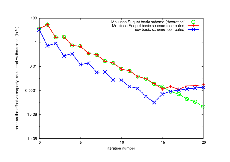
Figure 7: The results of Moulinec and Suquet (to be published) comparing the convergence of numerical results to the formula (7.1) for the effective conductivity $\sigma_{*}$ when $\sigma_{1}=0$ and $\sigma_{2}=1$, for their basic scheme (Moulinec and Suquet [27], [28]), and for the basic scheme applied in the Hilbert space ${\cal H}^{\prime\prime}$. Printed with permission of Hervé Moulinec and Pierre Suquet.

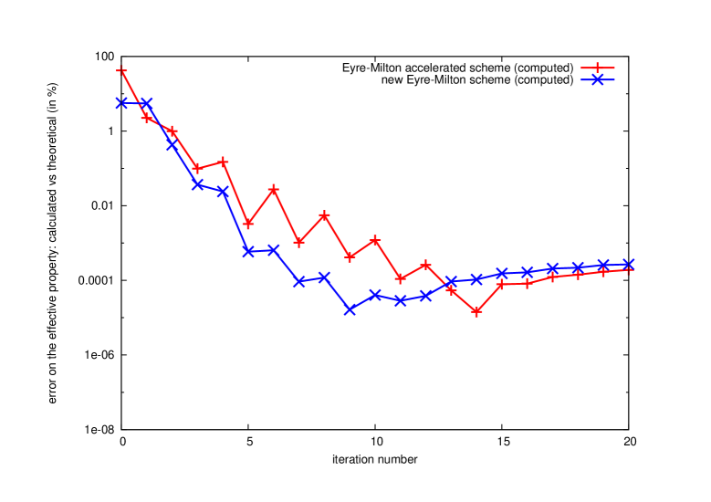
Figure 8: The results of Moulinec and Suquet (to be published) comparing the convergence of numerical results to the formula (7.1) for the effective conductivity $\sigma_{*}$, when $\sigma_{1}=0$ and $\sigma_{2}=1$ for the accelerated scheme of [7] (see also the generalization in section 14.9 of [21]), and for the accelerated scheme applied in the Hilbert space ${\cal H}^{\prime\prime}$. Printed with permission of Hervé Moulinec and Pierre Suquet

8 Estimating the parameters $\alpha$ and $\beta$

[4] has derived rigorous lower bounds on $\alpha$ and upper bounds on $\beta$, for suspensions of separated spheres in a medium. Actually we need only estimates on $\alpha$ and $\beta$. For instance if an estimate on $\alpha$ is slightly too large, then the transformations will look like those depicted in 9. The series will still converge but only for $|z|<c$, where $c$ will be close to $1$ (but less than $1$). However, the support of the measure will be highly dependent on small details of the microstructure: a tiny sharp cusp on the surface of an otherwise smooth inclusion will in general dramatically change the support of the measure: see [13], page 378 of [21], and equation (15) of [12]. As remarked on page 378 of [21], this is related to the fact that these sharp corners behave as sinks of energy in the mathematically equivalent dielectric problem with the conductivities $\sigma_{1}$ and $\sigma_{2}$ being replaced by electrical permittivities $\varepsilon_{1}$ and $\varepsilon_{2}$, where $\varepsilon_{2}$ is real and positive, while $\varepsilon_{1}$ is almost real and negative with a tiny positive imaginary part. Related observations and analysis include those of [34], [33], [6], and [3]. Also there is a close connection with the essential spectrum of the Neumann–Poincaré operator on planar domains with corners ([11]; [32]).

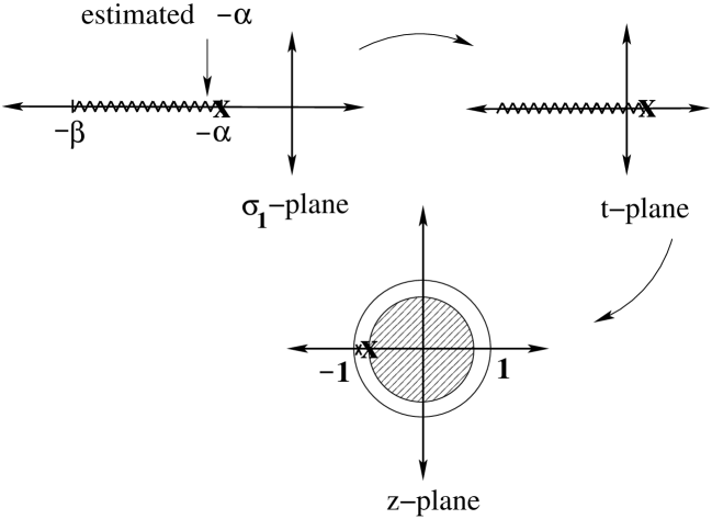
Figure 9: The new accelerated scheme should still work although not as effectively, even when we make a small error in the estimation of $\alpha$ (and/or $\beta$). With this error a singularity at ${\bf X}$, gets mapped to a point slightly greater than zero in the $t$-plane, and then gets mapped to a point slightly inside the unit disk in the $z$-plane. There is a consequent reduction in the radius of convergence, and an associated decrease in the rate of convergence, for the series in powers of $z$.

9 Bounds on the support of the measure using $Q^{*}_{C}$-convex functions

For many other equations in periodic composite materials robust things can be said about the measure which restrict its support. We assume we have a Hilbert space ${\cal H}$ of square integrable periodic fields ${\bf P}({\bf x})$ with an inner product

$$({\bf P}^{\prime},{\bf P})=\langle\overline{{\bf P}}^{\prime}\cdot{\bf P}\rangle,$$ (9.1)

where the angular brackets denote an average over the unit cell of periodicity. We also assume ${\cal H}$ has a decomposition into three orthogonal subspaces

$${\cal H}={\cal U}\oplus{\cal E}\oplus{\cal J}.$$ (9.2)

We are interested in the equations

$${\bf J}_{0}+{\bf J}({\bf x})={\bf L}({\bf x})({\bf E}_{0}+{\bf E}({\bf x})),$$ (9.3)

where

$${\bf J}_{0},{\bf E}_{0}\in{\cal U},\quad{\bf E}\in{\cal E},\quad{\bf J}\in{\cal J},$$ (9.4)

and where the local tensor field ${\bf L}({\bf x})$ takes the form

$${\bf L}({\bf x})={\bf Q}({\bf R}({\bf x}))\left[\sum_{i=1}^{n}\chi_{i}({\bf x}){\bf L}_{i}\right][{\bf Q}({\bf R}({\bf x}))]^{T},$$ (9.5)

in which ${\bf Q}({\bf R})$ is the orthogonal matrix (satisfying ${\bf Q}{\bf Q}^{T}={\bf I}$) associated with a rotation ${\bf R}$ acting on elements in the tensor space, while ${\bf R}({\bf x})$ is a field of rotation matrices giving the local orientation of each phase, and $\chi_{i}({\bf x})$ is the indicator function that is $1$ in phase $i$ and zero elsewhere.

First, following section 14.8 of [21] let us show that there are series expansions for the effective tensor that converge even when the local tensor ${\bf L}({\bf x})$ is not everywhere positive definite. To obtain the series expansion we introduce a constant reference tensor ${\bf L}_{0}$ and an associated operator ${\Gamma}$: we say

$${\bf E}^{\prime}=\mbox{\boldmath${\Gamma}$}{\bf P}\quad\text{if and only if }{\bf E}^{\prime}\in{\cal E}\text{ and }{\bf P}-{\bf L}_{0}{\bf E}^{\prime}\in{\cal U}\oplus{\cal J}.$$ (9.6)

Explicitly, ${\Gamma}$ is given by the operator

$$\mbox{\boldmath${\Gamma}$}=\mbox{\boldmath${\Gamma}$}_{1}(\mbox{\boldmath${\Gamma}$}_{1}{\bf L}_{0}\mbox{\boldmath${\Gamma}$}_{1})^{-1}\mbox{\boldmath${\Gamma}$}_{1},$$ (9.7)

where the inverse is to be taken on the subspace ${\cal E}$. Introducing the polarization field

$${\bf P}=({\bf L}-{\bf L}_{0})({\bf E}_{0}+{\bf E})={\bf J}_{0}+{\bf J}-{\bf L}_{0}({\bf E}_{0}+{\bf E}),$$ (9.8)

we see it satisfies $\mbox{\boldmath${\Gamma}$}{\bf P}=-{\bf E}$, and hence we have the identity

$$[{\bf I}+\mbox{\boldmath${\Gamma}$}({\bf L}-{\bf L}_{0})]({\bf E}_{0}+{\bf E})={\bf E}_{0}+{\bf E}-{\bf E}={\bf E}_{0},$$ (9.9)

which gives

$${\bf J}_{0}+{\bf J}={\bf L}({\bf E}_{0}+{\bf E})={\bf L}[{\bf I}+\mbox{\boldmath${\Gamma}$}({\bf L}-{\bf L}_{0})]^{-1}{\bf E}_{0}.$$ (9.10)

Averaging both sides yields a formula for the effective tensor, and associated series expansion:

$${\bf L}_{*}=\langle{\bf L}[{\bf I}+\mbox{\boldmath${\Gamma}$}({\bf L}-{\bf L}_{0})]^{-1}\rangle=\sum_{j=0}^{\infty}\langle{\bf L}[\mbox{\boldmath${\Gamma}$}({\bf L}_{0}-{\bf L})]^{j}\rangle,$$ (9.11)

where the angular brackets denote a volume average.

A sufficient condition for convergence is that the operator $\mbox{\boldmath${\Gamma}$}({\bf L}_{0}-{\bf L})$ has norm less than $1$. We take a reference tensor of the form

$${\bf L}_{0}=\sigma_{0}{\bf I}+{\bf L}_{0}^{\prime},$$ (9.12)

where the tensor ${\bf L}^{\prime}_{0}$ is assumed to be bounded and self-adjoint, but need not be positive definite. We are interested in seeing whether the expansion for the effective tensor converges when $\sigma_{0}$ is very large. Expanding the operator ${\Gamma}$ in powers of $1/\sigma_{0}$ gives

$$\mbox{\boldmath${\Gamma}$}=\mbox{\boldmath${\Gamma}$}_{1}(\mbox{\boldmath${\Gamma}$}_{1}{\bf L}_{0}\mbox{\boldmath${\Gamma}$}_{1})^{-1}\mbox{\boldmath${\Gamma}$}_{1}=\mbox{\boldmath${\Gamma}$}_{1}/\sigma_{0}-\mbox{\boldmath${\Gamma}$}_{1}{\bf L}_{0}^{\prime}\mbox{\boldmath${\Gamma}$}_{1}/\sigma_{0}^{2}+{\bf R}_{1},$$ (9.13)

with a remainder term

$${\bf R}_{1}=\sum_{j=2}^{\infty}\mbox{\boldmath${\Gamma}$}_{1}(-1)^{j}({\bf L}_{0}^{\prime}\mbox{\boldmath${\Gamma}$}_{1})^{j}/\sigma_{0}^{j+1}.$$ (9.14)

When $\sigma_{0}>\|{\bf L}_{0}^{\prime}\|$ this remainder term has norm satisfying the bound

$$\|{\bf R}_{1}\|\leq\sum_{j=2}^{\infty}\|{\bf L}_{0}^{\prime}\|^{j}/\sigma_{0}^{j+1}=\frac{\|{\bf L}_{0}^{\prime}/\sigma_{0}\|^{2}}{\sigma_{0}-\|{\bf L}_{0}^{\prime}\|}.$$ (9.15)

This gives us a bound on the norm of $\mbox{\boldmath${\Gamma}$}({\bf L}_{0}-{\bf L})$:

$$\|\mbox{\boldmath${\Gamma}$}({\bf L}_{0}-{\bf L})\| = \|(\mbox{\boldmath${\Gamma}$}_{1}/\sigma_{0}-\mbox{\boldmath${\Gamma}$}_{1}{\bf L}_{0}^{\prime}\mbox{\boldmath${\Gamma}$}_{1}/\sigma_{0}^{2}+{\bf R}_{1})(\sigma_{0}{\bf I}+{\bf L}_{0}^{\prime}-{\bf L})\|$$ (9.16)

$$= \|\mbox{\boldmath${\Gamma}$}_{1}[{\bf I}+({\bf L}_{0}^{\prime}-{\bf L}-{\bf L}_{0}^{\prime}\mbox{\boldmath${\Gamma}$}_{1})/\sigma_{0}]+{\bf R}_{2}\|$$

$$\leq \|{\bf I}+({\bf L}_{0}^{\prime}-{\bf L}-\mbox{\boldmath${\Gamma}$}_{1}{\bf L}_{0}^{\prime}\mbox{\boldmath${\Gamma}$}_{1})/\sigma_{0}\|+\|{\bf R}_{2}\|,$$

where

$${\bf R}_{2}\equiv{\bf R}_{1}(\sigma_{0}{\bf I}+{\bf L}_{0}^{\prime}-{\bf L})-\mbox{\boldmath${\Gamma}$}_{1}{\bf L}_{0}^{\prime}\mbox{\boldmath${\Gamma}$}_{1}({\bf L}_{0}^{\prime}-{\bf L})/\sigma_{0}^{2}.$$ (9.17)

Now we can find a $\sigma^{+}>\|{\bf L}_{0}^{\prime}\|$ such that for $\sigma_{0}>\sigma_{0}^{+}$,

$$\|(\sigma_{0}{\bf I}+{\bf L}_{0}^{\prime}-{\bf L})\|<2\sigma_{0},\quad\sigma_{0}-\|{\bf L}_{0}^{\prime}\|>\sigma_{0}/2.$$ (9.18)

Hence there exists a constant $\beta_{1}>0$ (independent of $\sigma_{0}$) such that

$$\|{\bf R}_{2}\| \leq \|{\bf R}_{1}\|\|(\sigma_{0}{\bf I}+{\bf L}_{0}^{\prime}-{\bf L})\|+\|\mbox{\boldmath${\Gamma}$}_{1}{\bf L}_{0}^{\prime}\mbox{\boldmath${\Gamma}$}_{1}({\bf L}_{0}^{\prime}-{\bf L})\|/\sigma_{0}^{2}$$ (9.19)

$$\leq 4\|{\bf L}_{0}^{\prime}/\sigma_{0}\|^{2}+\|\mbox{\boldmath${\Gamma}$}_{1}{\bf L}_{0}^{\prime}\mbox{\boldmath${\Gamma}$}_{1}({\bf L}_{0}^{\prime}-{\bf L})\|/\sigma_{0}^{2}\leq\beta_{1}/\sigma_{0}^{2}.$$

Now given any bounded operator ${\bf A}$ with adjoint ${\bf A}^{\dagger}$ and field ${\bf P}\in{\cal H}$ with $|{\bf P}|=1$ we have

$$|({\bf I}-{\bf A}/\sigma_{0}){\bf P}|^{2} = ({\bf P},({\bf I}-{\bf A}/\sigma_{0})^{\dagger}({\bf I}-{\bf A}/\sigma_{0}){\bf P}$$ (9.20)

$$= 1-({\bf P},({\bf A}+{\bf A}^{\dagger}){\bf P})/\sigma_{0}+({\bf P},{\bf A}^{\dagger}{\bf A}{\bf P})/\sigma_{0}^{2}$$

$$\leq 1-({\bf P},({\bf A}+{\bf A}^{\dagger}){\bf P})/\sigma_{0}+\|{\bf A}^{\dagger}{\bf A}\|/\sigma_{0}^{2},$$

and from the definition of the norm of an operator, this implies

$$\|{\bf I}-{\bf A}/\sigma_{0})\|=1+\|{\bf A}^{\dagger}{\bf A}\|/\sigma_{0}^{2}-\min_{\begin{subarray}{c}{\bf P}\in{\cal H}\\ |{\bf P}|=1\end{subarray}}({\bf P},({\bf A}+{\bf A}^{\dagger}){\bf P})/\sigma_{0}.$$ (9.21)

Setting ${\bf A}={\bf L}-{\bf L}_{0}^{\prime}+{\bf L}_{0}^{\prime}\mbox{\boldmath${\Gamma}$}_{1}$ we see there exists a constant $\beta_{2}>0$ such that for $\sigma_{0}>\sigma_{0}^{+}$,

$$\|\mbox{\boldmath${\Gamma}$}({\bf L}_{0}-{\bf L})\|\leq 1+\beta_{2}/\sigma_{0}^{2}-2\min_{\begin{subarray}{c}{\bf P}\in{\cal H}\\ |{\bf P}|=1\end{subarray}}({\bf P},({\bf L}_{S}-{\bf L}_{0}^{\prime}+\mbox{\boldmath${\Gamma}$}_{1}{\bf L}_{0}^{\prime}\mbox{\boldmath${\Gamma}$}_{1}){\bf P})/\sigma_{0},$$ (9.22)

where ${\bf L}_{S}=({\bf L}+{\bf L}^{\dagger})/2$. If the operator ${\bf L}_{S}-{\bf L}_{0}^{\prime}+\mbox{\boldmath${\Gamma}$}_{1}{\bf L}_{0}^{\prime}\mbox{\boldmath${\Gamma}$}_{1}$ is coercive in the sense that there exists a constant $\alpha^{\prime}>0$ such that

$${\bf L}_{S}-{\bf L}_{0}^{\prime}+\mbox{\boldmath${\Gamma}$}_{1}{\bf L}_{0}^{\prime}\mbox{\boldmath${\Gamma}$}_{1}>\alpha^{\prime}{\bf I},$$ (9.23)

then (9.22) implies

$$\|\mbox{\boldmath${\Gamma}$}({\bf L}_{0}-{\bf L})\|<1+\beta_{2}/\sigma_{0}^{2}-\alpha^{\prime}/\sigma_{0},$$ (9.24)

and this will surely be less than $1$ for sufficiently large $\sigma_{0}$. Furthermore suppose the constant tensor ${\bf L}_{0}^{\prime}$ is positive semi-definite on the subspace ${\cal E}$, i.e., the associated quadratic form

$$f({\bf A})=\overline{{\bf A}}\cdot{\bf L}_{0}^{\prime}{\bf A}$$ (9.25)

is $Q^{*}_{C}$-convex, meaning it satisfies

$$\langle f({\bf E})\rangle\geq 0,\quad\text{for all }{\bf E}\in{\cal E},$$ (9.26)

where the angular brackets denote a volume average over the unit cell $C$ of periodicity. Also suppose there exists a positive constant $\alpha^{\prime}$ such that

$$\mbox{\boldmath${\Gamma}$}_{1}{\bf L}_{0}^{\prime}\mbox{\boldmath${\Gamma}$}_{1}\geq 0,\quad{\bf L}_{S}>{\bf L}_{0}^{\prime}+\alpha^{\prime}{\bf I}.$$ (9.27)

Then (9.23) will be satisfied. Now each term in the series expansion for ${\bf L}_{*}$ will be a polynomial in the elements of the matrices ${\bf L}_{1},{\bf L}_{2}$,$\ldots$,${\bf L}_{n}$ and hence in the domain where the series expansion converges, the effective tensor will be an analytic function of these matrix elements. Hence the support of the measure must lie outside the region where ${\bf L}_{S}>{\bf L}_{0}^{\prime}$.

Note that the definition (9.26) is slightly different to the meaning of $Q^{*}_{C}$-convexity given in [22] as here we allow for the space ${\cal E}$ to contain certain fields whose volume average is not zero (as happens when we treat the Schrödinger equation, with sources and with the energy having an imaginary part: see sections 13.6 and 13.7 of [24]. When the fields in ${\cal E}$ satisfy homogeneous linear differential constraints, the condition (9.26) is easily reduced to an algebraic condition by taking Fourier transforms of (9.26). The projection onto the space ${\cal E}$ is given by projections $\mbox{\boldmath${\Gamma}$}_{1}({\bf k})$, that are local in Fourier space and (9.26) holds if an only if

$$\mbox{\boldmath${\Gamma}$}_{1}({\bf k}){\bf L}_{0}^{\prime}\mbox{\boldmath${\Gamma}$}_{1}({\bf k})\geq 0,$$ (9.28)

for all ${\bf k}$, including ${\bf k}=0$ if ${\cal E}$ contains fields whose volume average is not zero, i.e., $\mbox{\boldmath${\Gamma}$}_{1}(0)\neq 0$. As shown in [22] this is basically the same procedure as followed by Murat and Tartar ([36]; [29]; [37]) to obtain algebraic conditions for a quadratic function to be quasiconvex. For quadratic functions, quasiconvexity and $Q^{*}$-convexity are equivalent when the fields satisfy differential constraints involving derivatives of fixed order, but are not equivalent when the differential constraints have derivatives of mixed orders, as in time-harmonic wave-equations.

References

- [1] George A. Baker, Jr. and P. R. Graves-Morris. Padé Approximants: Basic Theory. Part I. Extensions and Applications. Part II, volume 13 & 14 of Encyclopedia of Mathematics and its Applications. Addison-Wesley, Reading, Massachusetts, 1981. With a foreword by Peter A. Carruthers.
- [2] David J. Bergman. The dielectric constant of a composite material — A problem in classical physics. Physics Reports, 43(9):377–407, July 1978.
- [3] Anne-Sophie Bonnet-Ben Dhia, Lucas Chesnel, and Xavier Claeys. Radiation condition for a non-smooth interface between a dielectric and a metamaterial. Mathematical Models and Methods in Applied Sciences, 23(9):1629–1662, August 2013.
- [4] Oscar P. Bruno. The effective conductivity of strongly heterogeneous composites. Proceedings of the Royal Society of London. Series A, Mathematical and Physical Sciences, 433(1888):353–381, 1991.
- [5] Richard V. Craster and Yurii V. Obnosov. Four-phase checkerboard composites. SIAM Journal on Applied Mathematics, 61(6):1839–1856, 2001.
- [6] Nasim Mohammadi Estakhri and Andrea Alù. Physics of unbounded, broadband absorption/gain efficiency in plasmonic nanoparticles. Physical Review B: Condensed Matter and Materials Physics, 87(20):205418, May 2013.
- [7] David J. Eyre and Graeme W. Milton. A fast numerical scheme for computing the response of composites using grid refinement. European Physical Journal. Applied Physics, 6(1):41–47, April 1999.
- [8] Kenneth M. Golden. The interaction of microwaves with sea ice. In George C. Papanicolaou, editor, Wave Propagation in Complex Media, volume 96 of IMA Volumes in Mathematics and its Applications, pages 75–94. Springer-Verlag, Berlin / Heidelberg / London / etc., 1998.
- [9] Kenneth M. Golden and George C. Papanicolaou. Bounds for effective parameters of heterogeneous media by analytic continuation. Communications in Mathematical Physics, 90(4):473–491, 1983.
- [10] Kenneth M. Golden and George C. Papanicolaou. Bounds for effective parameters of multicomponent media by analytic continuation. Journal of Statistical Physics, 40(5–6):655–667, September 1985.
- [11] Johan Helsing, Hyeonbae Kang, and Mikyoung Lim. Classification of spectrum of the Neumann–Poincaré operator on planar domains with corners by resonance: a numerical study. Preprint, 2016.
- [12] Johan Helsing, Ross C. McPhedran, and Graeme W. Milton. Spectral super-resolution in metamaterial composites. New Journal of Physics, 13(11):115005, 2011.
- [13] J. H. Hetherington and M. F. Thorpe. The conductivity of a sheet containing inclusions with sharp corners. Proceedings of the Royal Society of London. Series A, Mathematical and Physical Sciences, 438(1904):591–604, September 1992.
- [14] R. A. Lebensohn. -site modeling of a D viscoplastic polycrystal using Fast Fourier Transform. Acta Materialia, 49(14):2723–2737, August 2001.
- [15] S.-B. Lee, R. A. Lebensohn, and A. D. Rollett. Modeling the viscoplastic micromechanical response of two-phase materials using Fast Fourier Transforms. International Journal of Plasticity, 27(5):707–727, May 2011.
- [16] Ross C. McPhedran and Graeme W. Milton. Bounds and exact theories for the transport properties of inhomogeneous media. Applied Physics A: Materials Science & Processing, 26(4):207–220, December 1981.
- [17] Graeme W. Milton. Theoretical studies of the transport properties of inhomogeneous media. Unpublished report TP/79/1, University of Sydney, Sydney, Australia, 1979.
- [18] Graeme W. Milton. Bounds on the complex permittivity of a two-component composite material. Journal of Applied Physics, 52(8):5286–5293, August 1981.
- [19] Graeme W. Milton. Bounds on the transport and optical properties of a two-component composite material. Journal of Applied Physics, 52(8):5294–5304, August 1981.
- [20] Graeme W. Milton. Proof of a conjecture on the conductivity of checkerboards. Journal of Mathematical Physics, 42(10):4873–4882, October 2001.
- [21] Graeme W. Milton. The Theory of Composites, volume 6 of Cambridge Monographs on Applied and Computational Mathematics. Cambridge University Press, Cambridge, UK, 2002. Series editors: P. G. Ciarlet, A. Iserles, Robert V. Kohn, and M. H. Wright.
- [22] Graeme W. Milton. Sharp inequalities that generalize the divergence theorem: an extension of the notion of quasi-convexity. Proceedings of the Royal Society A: Mathematical, Physical, & Engineering Sciences, 469(2157):20130075, 2013. See addendum [Milton:2015:ATS].
- [23] Graeme W. Milton and Ross C. McPhedran. A comparison of two methods for deriving bounds on the effective conductivity of composites. In Robert Burridge, Stephen Childress, and George C. Papanicolaou, editors, Macroscopic Properties of Disordered Media: Proceedings of a Conference Held at the Courant Institute, June 1–3, 1981, volume 154 of Lecture Notes in Physics, pages 183–193, Berlin / Heidelberg / London / etc., 1982. Springer-Verlag.
- [24] Graeme W. Milton (editor). Extending the Theory of Composites to Other Areas of Science. Milton–Patton Publishers, P.O. Box 581077, Salt Lake City, UT 85148, USA, 2016.
- [25] Stefano Mortola and Sergio Steffé. A two-dimensional homogenization problem. (Italian). Atti della Accademia Nazionale dei Lincei. Rendiconti. Classe di Scienze Fisiche, Matematiche e Naturali. Serie VIII, 78(3):77–82, 1985.
- [26] H. Moulinec and F. Silva. Comparison of three accelerated FFT-based schemes for computing the mechanical response of composite materials. International Journal for Numerical Methods in Engineering, 97(13):960–985, March 2014.
- [27] H. Moulinec and Pierre M. Suquet. A fast numerical method for computing the linear and non-linear properties of composites. Comptes rendus des Séances de l’Académie des sciences. Série II, 318(??):1417–1423, 1994.
- [28] H. Moulinec and Pierre M. Suquet. A numerical method for computing the overall response of non-linear composites with complex microstructure. Computer Methods in Applied Mechanics and Engineering, 157(1–2):69–94, 1998.
- [29] François Murat and Luc Tartar. Calcul des variations et homogénísation. (French) [Calculus of variation and homogenization]. In Les méthodes de l’homogénéisation: théorie et applications en physique, volume 57 of Collection de la Direction des études et recherches d’Électricité de France, pages 319–369, Paris, 1985. Eyrolles. English translation in Topics in the Mathematical Modelling of Composite Materials, pp. 139–173, ed. by A. Cherkaev and R. Kohn, ISBN 0-8176-3662-5.
- [30] Yurii V. Obnosov. Periodic heterogeneous structures: New explicit solutions and effective characteristics of refraction of an imposed field. SIAM Journal on Applied Mathematics, 59(4):1267–1287, 1999.
- [31] Chris Orum, Elena Cherkaev, and Kenneth M. Golden. Recovery of inclusion separations in strongly heterogeneous composites from effective property measurements. Proceedings of the Royal Society of London. Series A, Mathematical and Physical Sciences, 468(2139):784–809, January 2012.
- [32] Karl-Mikael Perfekt and Mihai Putinar. The essential spectrum of the Neumann–Poincaré operator on a domain with corners. Archive for Rational Mechanics and Analysis, 223(2):1019–1033, February 2017.
- [33] M. Pitkonen. A closed-form solution for the polarizability of a dielectric double half-cylinder. Journal of Electromagnetic Waves and Applications, 24(8–9):1267–1628, 2010.
- [34] Cheng-Wei Qiu and B. Luk’yanchuk. Peculiarities in light scattering by spherical particles with radial anisotropy. Journal of the Optical Society of America. A, Optics, image science, and vision, 25(7):1623–1628, 2008.
- [35] Romuald Sawicz and Kenneth M. Golden. Bounds on the complex permittivity of matrix-particle composites. Journal of Applied Physics, 78(12):7240–7246, December 1995.
- [36] Luc Tartar. Compensated compactness and applications to partial differential equations. In R. J. Knops, editor, Nonlinear Analysis and Mechanics, Heriot–Watt Symposium, Volume IV, volume 39 of Research Notes in Mathematics, pages 136–212, London, 1979. Pitman Publishing Ltd.
- [37] Luc Tartar. Estimations fines des coefficients homogénéisés. (French) [Fine estimations of homogenized coefficients]. In P. Krée, editor, Ennio de Giorgi Colloquium: Papers Presented at a Colloquium Held at the H. Poincaré Institute in November 1983, volume 125 of Pitman Research Notes in Mathematics, pages 168–187, London, 1985. Pitman Publishing Ltd.
- [38] François Willot. Fourier-based schemes for computing the mechanical response of composites with accurate local fields. Comptes rendus mécanique, 343(3):232–245, March 2015.
- [39] François Willot, Bassam Abdallah, and Yves-Patrick Pellegrini. Fourier-based schemes with modified Green operator for computing the electrical response of heterogeneous media with accurate local fields. International Journal for Numerical Methods in Engineering, 98(7):518–533, May 2014.