Dynamics of extended Schelling models

Abstract

We explore extensions of Schelling’s model of social dynamics, in which two types of agents live on a checkerboard lattice and move in order to optimize their own satisfaction, which depends on how many agents among their neighbors are of their same type. For each number $n$ of same-type nearest neighbors we independently assign a binary satisfaction variable $s_{k}$ which is equal to one only if the agent is satisfied with that condition, and is equal to zero otherwise. This defines 32 different satisfaction rules, which we investigate in detail, focusing on pattern formation and measuring segregation with the help of an “energy” function which is related to the number of neighboring agents of different types and plays no role in the dynamics. We consider the checkerboard lattice to be fully occupied and the dynamics consists of switching the locations of randomly selected unsatisfied agents of opposite types. We show that, starting from a random distribution of agents, only a small number of rules lead to (nearly) fully segregated patterns in the long run, with many rules leading to chaotic steady-state behavior. Nevertheless, other interesting patterns may also be dynamically generated, such as “anti-segregated” patterns as well as patterns resembling sponges.

1 Introduction

Aiming at studying racial segregation in American cities, Schelling formulated one the first mathematical models of social agents around 50 years ago [1, 2]. The spirit of Schelling’s model can be summarized by the presence of two types of agents occupying the sites of a network and able to move seeking to optimize their satisfaction, which is determined by how many agents of their same type are located in their neighborhood. As shown by Schelling, the model predicts that only a minor preference of the agents for neighbors of their same type leads to segregation.

Apart from many applications to study segregation in other fields such as biology and economy (see e.g. Ref. [3] and references therein), as well as to determine the robustness of Schelling’s model predictions under a change of network topology [4, 5], different versions of the model have attracted the attention of physicists for the last 15 years (see e.g. Refs. [6, 7, 8, 9, 10, 11, 12, 13, 3, 14, 15, 16]), following a similar interest in investigating social dynamics using a variety of statistical-physics models [17, 18, 19, 20, 21]. Due to the fact that the dynamics of such models is determined by the optimization of individual variables rather than collective variables such as the energy, the methods of equilibrium statistical mechanics are hardly useful, and mostly computer simulations are employed. In order to make analytical progress in investigating Schelling-like models, one has to look at coarse-grained versions [10, 14, 16, 22] involving extended neighborhoods or to perform more radical approximations such as making assumptions about the long-time behavior [8] or imposing that each agent has a single neighbor [3].

Most approaches based on Schelling’s model focus on appearance of segregation, varying the fraction of vacant sites or the minimum tolerated fraction of neighboring agents of the same type. In contrast, here we do not restrain ourselves to cases directly inspired by the desire to model the appearance of segregation in social systems, but rather, inspired by nonequilibrium statistical-physics models [23, 24], we explore the dynamic variability of extensions of Schelling’s model in which for each number $n$ of same-type neighbors we independently assign a binary satisfaction variable $s_{k}$ which is equal to one only if the agent is satisfied with that condition, and is equal to zero otherwise. This defines 32 distinct satisfaction rules, which we investigate in detail, focusing on pattern formation and measuring segregation with the help of an “energy” function which is related to the number of neighboring agents of different types and plays no role in the dynamics. The model is defined on a square lattice with no vacancies and a given agent interacts with the 4 agents in its von-Neumann neighborhood, rather than with the 8 agents in its Moore neighborhood, as in Schelling’s original model. The dynamics consists of switching the locations of randomly selected unsatisfied agents of opposite types. Although most of our results are obtained through simulations, we also provide a few analytical estimates.

We show that, starting from a random distribution of agents, only a small number of rules lead to (nearly) fully segregated patterns in the long run, with many rules leading to chaotic steady-state behavior. Nevertheless, other interesting patterns may also be dynamically generated, such as “anti-segregated” patterns as well as patterns resembling sponges. A crucial role in the dynamics is played by the existence of fixed points, which are equivalent to the absorbing states familiar in the nonequilibrium statistical-physics literature [23, 24]. This is detailed in the next section.

2 The models

We assume that two types of agents — which we call “blue” (or type 0) and “red” (or type 1) agents — fully occupy the sites of a $L\times L$ square lattice (subject to periodic boundary conditions), with half of the sites randomly occupied by each type of agent. Each agent interacts with the 4 agents in its von-Neumann neighborhood. The satisfaction of each agent depends on the number of agents of its same type in its neighborhood, so that the model would correspond to a (asynchronous) totalistic automaton [25]. A parameter of the model is the five-digit binary number $s=s_{0}s_{1}s_{2}s_{3}s_{4}$, with $s_{n}=1$ indicating that an agent is satisfied having $n$ neighbors of its same type, and $s_{n}=0$ otherwise. We take the satisfaction parameter to be the same for both types of agents, and we refer to a given satisfaction parameter as defining the satisfaction rule of the dynamics. Schelling’s original model of segregation [1, 2] would be closer to rule $00111$, while rules 00000, 00001, 00011, 00111 and 01111 were also investigated in Ref. [13].

In many formulations of Schelling’s model, including his own, the dynamics prescribes that an unsatisfied agent moves to a vacant site. As our model has no vacancies, we assume that the basic step of the dynamics is implemented by randomly selecting two unsatisfied agents, one of each type, and switching their locations, irrespective of whether the agents become satisfied in their new locations, and irrespective of the original distance between the agents. We implement this dynamics for a maximum of $10^{5}$ Monte Carlo (MC) sweeps, with a single MC sweep corresponding to $L^{2}$ basic steps. (Keep in mind that two agents always switch location at each basic step.) In this Section we investigate the effect of all satisfaction rules on the long-time behavior of the system. The rule 11111 is trivial, as it does not allow for the existence of unsatisfied agents, thus having no dynamics, and will not be further discussed. We are then left with 31 distinct rules.

We measure time in units of the inverse number of unsatisfied agents, which means that the time increments between consecutive simulation steps are nonuniform, being given by

$$\Delta t=\frac{1}{N_{u,1}+N_{u,0}},$$ (1)

in which $N_{u,c}$ represents the number of unsatisfied agents of type $c\in\{0,1\}$. We follow the time evolution of the fraction of unsatisfied agents,

$$\rho_{u}=\frac{N_{u,1}+N_{u,0}}{L^{2}},$$ (2)

and of an “energy” function defined as

$$E=-\sum_{\left\langle i,j\right\rangle}\left(2c_{i}-1\right)\left(2c_{j}-1\right),$$ (3)

in which the sum is over all neighboring pairs of agents and $c_{i}=0$ ($c_{i}=1$) if a blue (red) agent occupies site $i$. The energy function, which is related to the interface density of Refs. [8, 11, 3, 14], has its maximum value ($E_{\text{max}}=2L^{2}$) when the agents arrange themselves in a checkerboard 1x1 pattern, for which all agents only have neighbors of the opposite type, while the minimum value ($E_{\text{min}}=-2L^{2}+4L)$ corresponds to complete segregation, in which there are two uniform domains, each containing all the agents of a given type. Values of $E$ close to zero indicate the existence of various static or dynamic local patterns in different regions of the system. For some rules, along the lines of Ref. [13], the energy function can be shown to be either monotonically nonincreasing or nondecreasing in time, which is useful in the discussion of the possible long-time behaviors. We also calculate the survival probability $P_{s}\left(t\right)$, defined as the average fraction of simulations which do not freeze (as defined below) before time $t$.

There are three possible cases for the qualitative long-time dynamics, with finer details to be discussed later: (i) the dynamics freezes after a finite number of steps, with all agents of at least one type satisfied and zero survival probability at long times; (ii) a large fraction of the agents become satisfied after a finite number of steps, with a small fraction of unsatisfied agents (necessarily of both types) making the dynamics persist indefinitely, reaching a nonzero survival probability as $t\rightarrow\infty$; (iii) no agent becomes permanently satisfied, and the dynamics persists indefinitely in an essentially chaotic manner, with temporary pockets of satisfied agents, again with a nonzero long-time survival probability.

For cases (i) and (ii) the behavior is associated with the existence and stability of “equilibrium” states — fixed points of the dynamics, in which all agents are satisfied — corresponding to a given satisfaction rule. Depending on the rule, there may be a huge number of fixed points (called “absorbing states” in the nonequilibrium phase transitions literature [23]), including several which correspond to irregular arrangements. We list below the simplest regular fixed points (FPs).

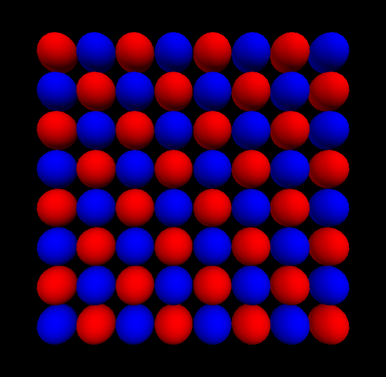
(a)

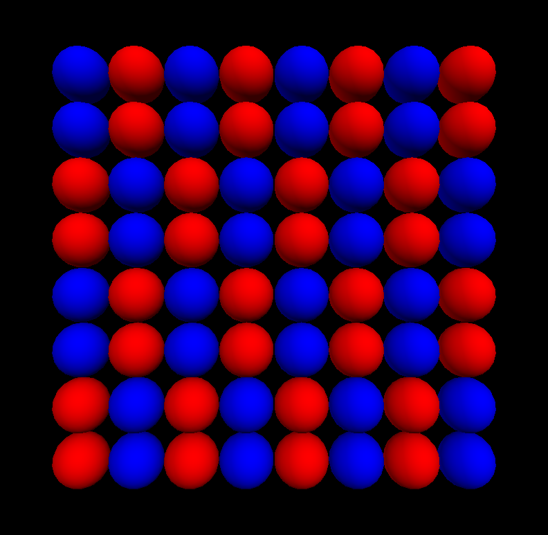
(b)

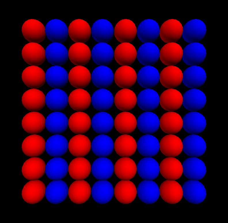
(c)

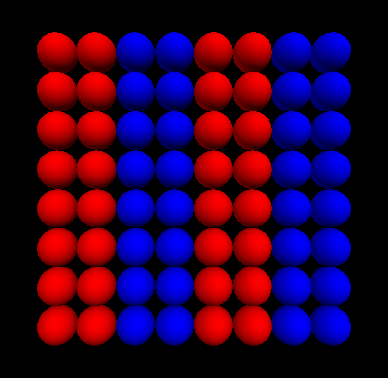
(d)

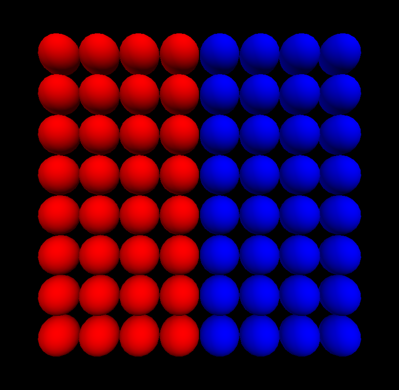
(e)

Figure 1: Some regular fixed points of the rules defined in Sec. 2.

(1) A checkerboard 1x1 pattern, illustrated in Fig. 1(a), in which a blue agent is surrounded by four red agents, and vice-versa. This pattern is a FP for rules of the form $1s_{1}s_{2}s_{3}s_{4}$, i.e. all rules under which an agent is satisfied having no neighbors of its same type.

(2) A checkerboard 1x2 pattern, illustrated in Fig. 1(b), in which a pair of neighboring blue agents is surrounded by six red agents, and vice-versa. This pattern is a FP for rules of the form $s_{0}1s_{2}s_{3}s_{4}$, under which an agent is satisfied having only one neighbor of its same type.

(3) A striped pattern, illustrated in Fig 1(c), in which a single line (or column) of blue agents is surrounded by two lines (or columns) of red agents, and vice-versa. This pattern is a FP for rules of the form $s_{0}s_{1}1s_{3}s_{4}$, under which an agent is satisfied having two neighbors of its same type.

(4) A double striped pattern, illustrated in Fig 1(d), in which a double line (or column) of blue agents is surrounded by two double lines (or columns) of red agents, and vice-versa. This pattern is a FP for rules of the form $s_{0}s_{1}s_{2}1s_{4}$, under which an agent is satisfied having three neighbors of its same type.

(5) A fully segregated pattern, illustrated in Fig. 1(e), in which there are only two uniform domains of agents of each type, separated by two linear boundaries (due to our choice of periodic boundary conditions). This pattern is a FP for rules of the form $s_{0}s_{1}s_{2}11$, under which an agent is satisfied having either three or four neighbors of its same type.

We investigated the stability of the above FPs with respect to small perturbations, introducing typically 1 to 8 “defect” agents of each type by switching the positions of randomly chosen agents of opposite types in order to disturb the FP arrangement. It turns out that in most cases the dynamics does not take the system arbitrarily away from the FPs, with the steady-state configurations resembling the arrangement of agents in the FP, but with a relatively small fraction of defects, especially when some of these are satisfied at their new positions. This fraction of defects turns out to be zero, so that the FP is fully stable, for rules $00011$ [around FP (5)], $00110$ [around FP (4)], $00111$ [around FP (4)], $01100$ [around FP (2)], $01110$ [around FP (4)], $10111$ [around FP (4)], $11000$ [around FP (1)], $11010$ [around FP (1)], $11100$ [around FPs (1) and (2)], $11101$ [around FP (2)], and $11110$ [around FP (1)]. In other cases the FPs are fully unstable, and the steady-state configuration bears no resemblance to the FP arrangement. This full instability happens for rules $00010$ [around FP (4)], $00100$ [around FP (3)], $00101$ [around FP (3)], $01000$ [around FP (2)], $01010$ [around both FPs (2) and (4)], $01011$ [only around FP (2)], $10000$ [around FP (1)], $10001$ [around FP (1)], $10010$ [around both FPs (1) and (4)], $10100$ [around both FPs (1) and (3)], $10101$ [around both FPs (1) and (3)], $10110$ [only around FP (1)], and $11010$ [only around FP (4)].

However, we are more interested in whether the above regular FPs can be reached starting from random initial conditions. This happens only for the checkerboard 1x1 and the fully segregated patterns, but under most rules for which these FPs are stable the dynamics leads a finite system to the neighborhood of the FP without ever precisely reaching it. This is a consequence of the fact that, besides the regular fixed points listed above, there are also many other competing irregular fixed points, as well as configurations in which defects become trapped, giving rise to dynamic patterns (blinkers) in which the positions of unsatisfied agents alternate between a few positions.

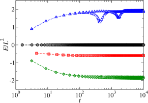
(a)

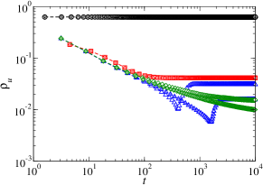
(b)

Figure 2: Time dependence of (a) the average energy function per agent and (b) the average fraction of unsatisfied agents for rules representing the four different possible long-time behaviors: chaotic (rule 00100, black circles), sponge-like (rule 00110, red squares), segregated (rule 01011, green diamonds), and checkerboard 1x1 (rule 11010, blue triangles). Open symbols (connected by dashed lines) correspond to system size $L=64$, while filled symbols correspond to $L=128$. Averages taken over at least 1000 initial conditions. Error bars are smaller than the symbols. Notice that for both rules 00100 and 00110 the curves for $L=64$ and $L=128$ are almost indistinguishable, while finite-size effects are relevant for rules 01011 and 11010.

With respect to pattern formation, starting from random initial conditions, the long-time behavior of the system strongly depends on the satisfaction rule. The possible qualitatively distinct outcomes correspond to (i) chaotic steady states; (ii) segregated states; (iii) checkerboard 1x1 states; (iv) sponge-like states. In what follows we discuss each of these possible outcomes. With the exceptions of rules $01011$, $10110$ and $11010$, which are unstable only around one of their fixed points, those rules which are unstable around their fixed points evolve to chaotic steady states, as described below. Examples of the time dependence of the energy function and of the fraction of unsatisfied agents for the distinct outcomes are shown in Fig. 2.

Chaotic steady states

Rule $s$	00000	00001	00010	00100	00101	01010	01001
$E^{\text{(sim)}}/L^{2}$	$0.00$	$-0.209$	$-0.374$	$0.00$	$-0.219$	$0.00$	$+0.231$
$\rho_{u}^{\text{(sim)}}$	$1.00$	$0.895$	0.627	$0.625$	$0.524$	$0.500$	$0.587$
$\rho_{u}^{\text{(MF)}}$	$1$	$0.9375$	$0.75$	$0.625$	$0.5625$	$0.5$	$0.6875$

Rule $s$	10001	10000	01000	11011	10100	10101	10010
$E^{\text{(sim)}}/L^{2}$	$0.00$	$+0.209$	$+0.373$	$\sim t/L^{2}$	$+0.219$	$0.00$	$-0.230$
$\rho_{u}^{\text{(sim)}}$	$0.875$	$0.895$	$0.627$	$0.375$	$0.524$	$0.500$	$0.586$
$\rho_{u}^{\text{(MF)}}$	$0.875$	$0.9375$	$0.75$	$0.375$	$0.5625$	$0.5$	$0.6875$

Table 1: The 14 rules leading to chaotic steady states starting from random initial conditions. Simulation results for the energy per agent $E^{\text{(sim)}}/L^{2}$ and the fraction $\rho_{u}^{\text{(sim)}}$ of unsatisfied agents correspond to long-time averages over 1000 initial conditions. The uncertainty in the simulation results is in the last digit. Results for the mean-field fraction $\rho_{u}^{\text{(MF)}}$ of unsatisfied agents have no uncertainty, and come from Eq. (4). See main text for a discussion on the behavior of the energy for rule 11011.

There are 14 rules under which the long-time survival probability is 100% and no stable macroscopic domains of satisfied agents are produced after a finite time in the thermodynamic limit. These rules are listed in Table 1, along with the corresponding stationary average total fraction of unsatisfied agents, $\rho_{u}$. Since there are no macroscopic domains of satisfied agents, these fractions can be compared with mean-field-like estimates obtained by neglecting short-range correlations between agents. The reasoning is based on counting the number of ways a given agent can have $k$ neighboring agents of its same type, and taking into account the corresponding probabilities. As the total number of agents of both types is the same, the steady-state fraction of unsatisfied agents (of both types) is given by

$$\rho_{u}^{\text{(MF)}}\left(s\right)=\left(\frac{1}{2}\right)^{4}\sum_{k=0}^{4}\left(1-s_{k}\right)\frac{4!}{k!\left(4-k\right)!},$$ (4)

in which $s=s_{0}s_{1}s_{2}s_{3}s_{4}$ defines the rule. See the Appendix for a derivation of the above result.

On the other hand, this mean-field approximation, which is based on the assumption that all configurations of the neighborhood of any agent are equally probable, predicts that the average energy function would be zero for all rules, and this is not generally compatible with the square-lattice simulations. Table 1 also shows simulation results for the energy per agent $E/L^{2}$, as well as a comparison between the mean-field estimates $\rho_{u}^{\text{(MF)}}$ and the simulation results $\rho_{u}^{\text{(sim)}}$ for the fraction of unsatisfied agents. Notice that in general there is good agreement between $\rho_{u}^{\text{(MF)}}$ and $\rho_{u}^{\text{(sim)}}$, with a relative discrepancy below 15%. For both $\rho_{u}^{\text{(MF)}}$ and $\rho_{u}^{\text{(sim)}}$, there is a symmetry in the steady-state fraction of unsatisfied agents between a rule $s=s_{0}s_{1}s_{2}s_{3}s_{4}$ and its mirror rule $s^{\prime}=s_{4}s_{3}s_{2}s_{1}s_{0}$; see the Appendix for a justification of this statement for any regular lattice. Notice as well that, within numerical errors, $E\left(s^{\prime}\right)=-E\left(s\right)$, if $s^{\prime}\neq s$, a result which is also justified in the Appendix.

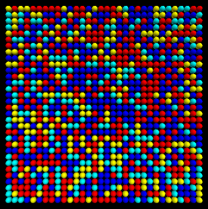
(a)

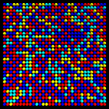
(b)

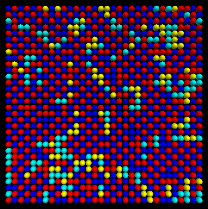
(c)

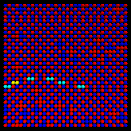
(d)

Figure 3: Snapshots of the time evolution of the system under rule 11011 and $L=32$. Unsatisfied agents are shown in lighter colors (yellow for red agents, cyan for blue agents). (a) The initial state, with energy per agent close to zero. (b) Configuration when $E/L^{2}\simeq 0.5$. (c) Configuration when $E/L^{2}\simeq 1.1$. (d) Configuration when $E/L^{2}=1.625$, the steady-state value for that particular simulation, in which the unsatisfied agents are blinkers (unsatisfied agents whose type alternates in time). Starting from random initial conditions, the time required to reach this kind of steady state diverges as $L\rightarrow\infty$.

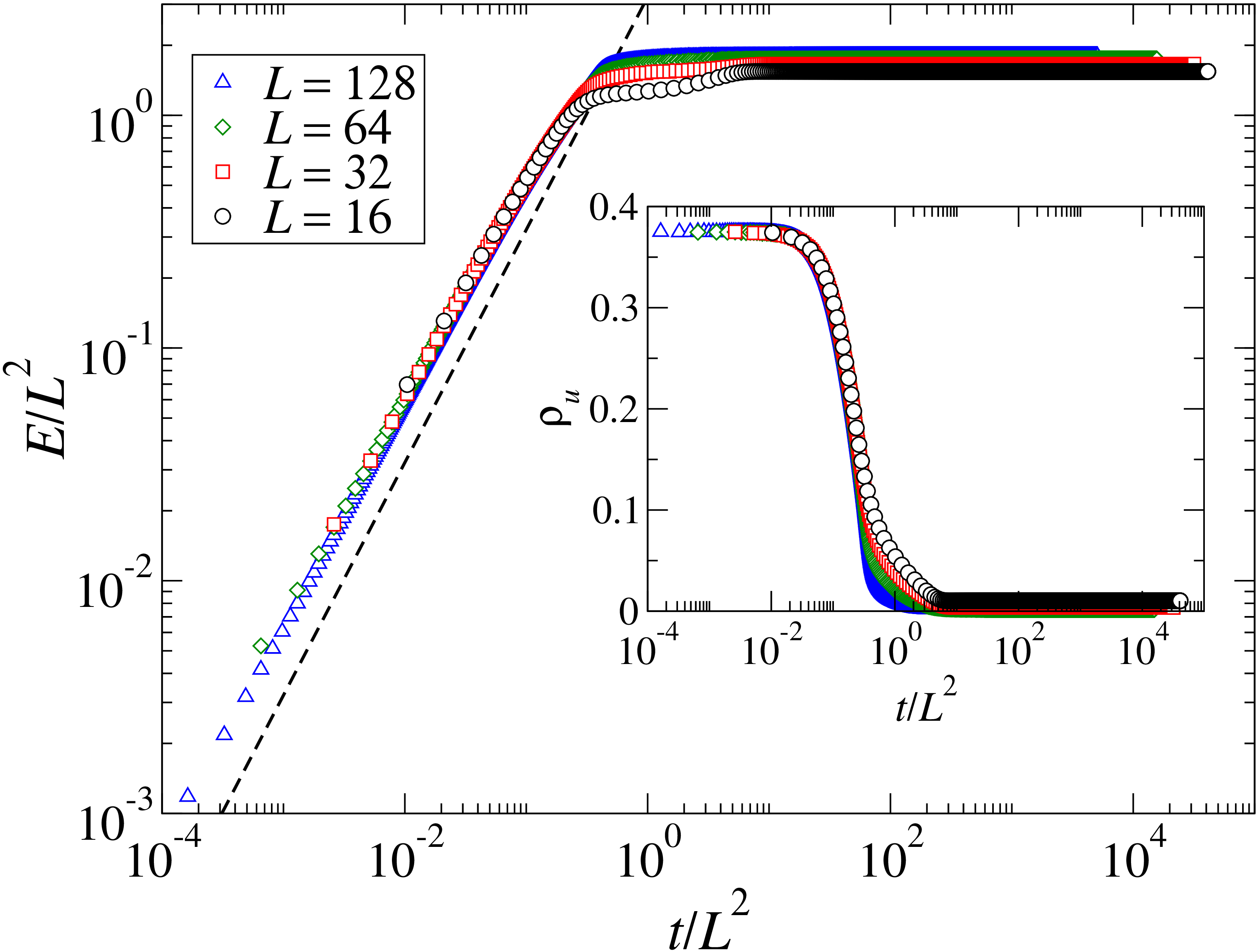
(a)

Figure 4: Main panel: energy per agent as a function of time (rescaled by $L^{2}$) under rule 11011, for various system sizes. The dashed line is proportional to $t/L^{2}$. Inset: fraction of unsatisfied agents as a function of $t/L^{2}$. Error bars are smaller than the symbols.

For mirror-symmetric rules, which are those for which $s^{\prime}=s$, it is also clear from Table 1 that the mean-field predictions for $\rho_{u}$ and $E$ seem to be exact, which is related to the fact that mirror-symmetry favors equal steady-state probabilities $p_{k}$ and $p_{4-k}$ for neighborhood configurations of an unsatisfied agent containing $k$ or $4-k$ agents of its opposite type, as well as equal corresponding probabilities $q_{k}$ and $q_{4-k}$ for a satisfied agent. For these pairs of configurations, the satisfaction state of the agent is the same and the local contributions to the energy function are $E_{k}$ and $E_{4-k}=-E_{k}$. However, in the case of the energy function, rule $11011$ is an exception, due to the fact that the stability of FP (1) under rule $11011$ is related to an spontaneous symmetry breaking between $q_{k}$ and $q_{4-k}$ for $k\neq 2$. Rule $11011$ is peculiar in that, for finite systems of linear size $L$, a seemingly chaotic state, for which the average energy nevertheless grows linearly with time, changes, after a timescale which grows as $L^{2}$, to a checkerboard 1x1 pattern with defects. Thus, in the thermodynamic limit the chaotic state is the only one to be observed. Figure 3 illustrates the behavior for a system with $L=32$, while Fig. 4 shows the time dependence of the average energy per agent and the average fraction $\rho_{u}$ of unsatisfied agents for different system sizes. As both the segregated state and the checkerboard 1x1 state are fixed points of the rule, a random initial condition can be considered as a mixture of checkerboard 1x1 and uniform domains of either type of agent, separated by clusters of unsatisfied agents. Under the dynamics, the average energy grows linearly with time, while $\rho_{u}$ remains essentially constant, so that domains of satisfied agents forming a local checkerboard 1x1 pattern grow in size by merging with each other, quickly outcompeting uniform domains. This is associated with the fact that, under this rule, agents are only unsatisfied if they have exactly two neighbors of their same type. Direct inspection of the possible local configurations makes it clear that the energy cannot decrease under the dynamics, and in fact it only increases (always by the same amount $\Delta E=6$) when two neighboring unsatisfied agents (of opposite types) are interchanged. This initially happens with a probability proportional to the inverse square of the number of unsatisfied agents times the number of clusters of unsatisfied agents, and therefore proportional to $L^{2}/L^{4}=L^{-2}$, so that the average number of steps required for the energy to increase by $\Delta E$ is proportional to $L^{2}$, which means a time interval of order one. Thus, in order to reach the maximum allowed value of the energy, which is proportional to $L^{2}$, a time of order $L^{2}$ is required. This can only be reached in finite systems.

Segregated states

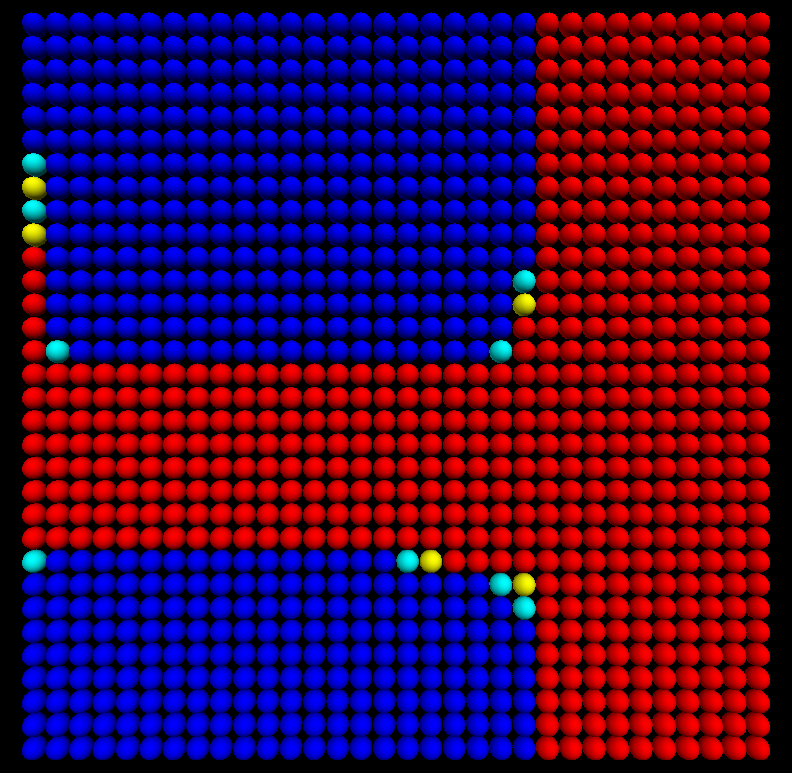
(a)

(b)

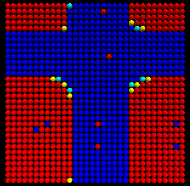
(c)

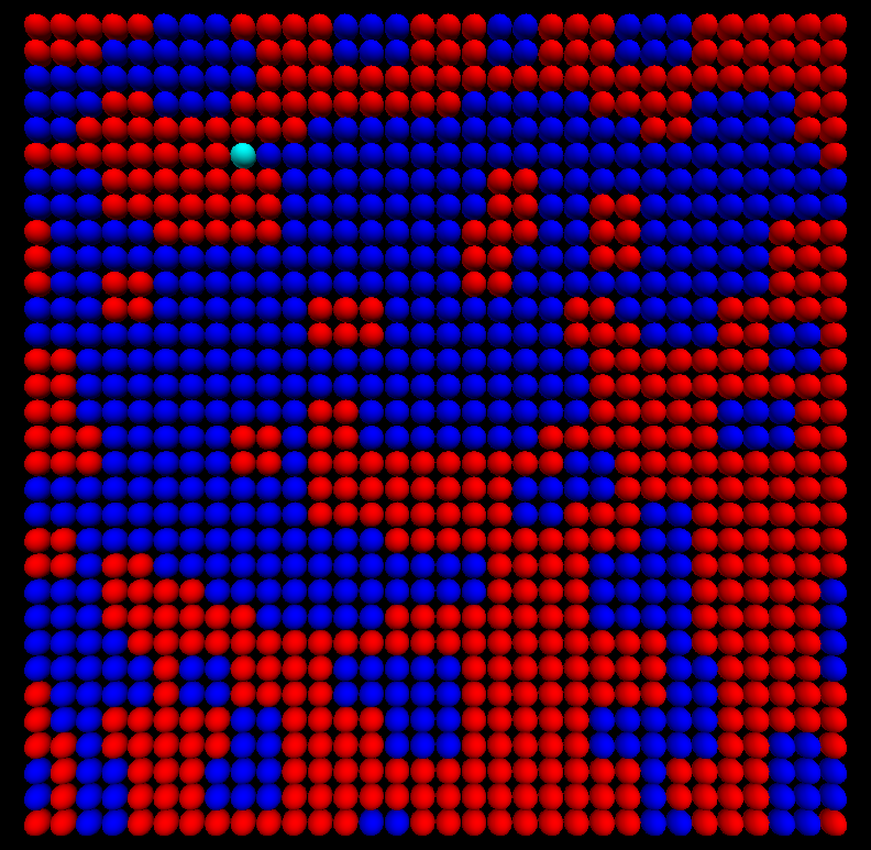
(d)

Figure 5: Examples of long-time configurations obtained for systems with $L=32$ under rules (a) 00011, (b) 01011, (c) 10011, which give rise to nearly fully segregated configurations, and (d) under rule 00111, for which the final pattern resembles a wide sponge. Color code is the same as in Fig. 3.

Under rules 00011, 01011 and 10011, the dynamics leads the system to a segregated state with two domains, one for each type of agent, possibly with a small number of “defect” static agents of the opposite type. The domains are usually separated by a small fraction of unsatisfied agents which goes to zero in the thermodynamic limit, as they sit at the domain boundaries and therefore their number scales at most with $L$, whereas the number of agents scales as $L^{2}$. We therefore expect that the long-time average fraction of unsatisfied agents $\rho_{u}$ decays as $1/L$, as long as the survival probability $P_{s}$$\left(t\rightarrow\infty\right)$ is $100\%$. However, under rule 00011 there is the possibility of forming perfectly linear domain boundaries containing only satisfied agents, in which case the dynamic freezes, so that $P_{s}\left(t\rightarrow\infty\right)$ is less than unity. This becomes increasingly unlikely in the thermodynamic limit, due to competition between horizontal and vertical boundaries, and $P_{s}\left(t\rightarrow\infty\right)$ seems to approach unity as $L\rightarrow\infty$, but rather slowly, leading to a slightly faster decay of $\rho_{u}$ as $L^{-1.1}$. Figures 5(a)-(c) show examples of long-time configurations for the three segregating rules.

For finite times and in the large $L$ regime, the fraction of unsatisfied agents decays roughly as $\rho_{u}\left(t\right)\sim 1/\sqrt{t}$ under the three rules. This is somewhat surprising, as, except for rule 00011, in which agents have a strict preference for a neighborhood containing a majority of agents of the same type, the other two rules yielding segregated patterns are more tolerant to agents of the opposite type, making an agent satisfied also if it has no neighbor (rule 10011) or a single neighbor (rule 01011) of its same type. However, this increased tolerance still leads to nearly fully segregated patterns in the long run.

Checkerboard 1x1 states

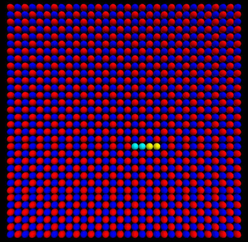
(a)

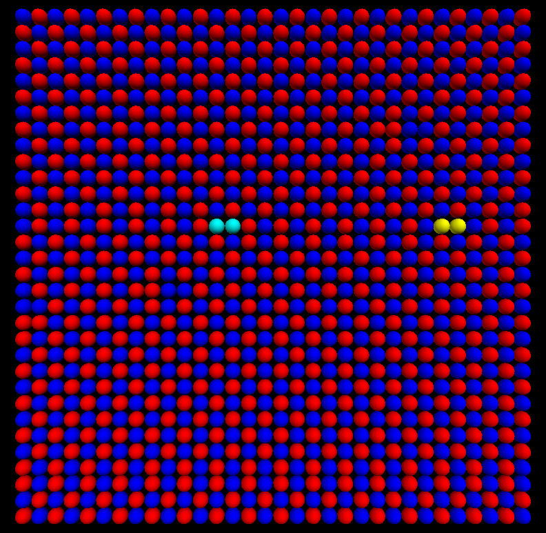
(b)

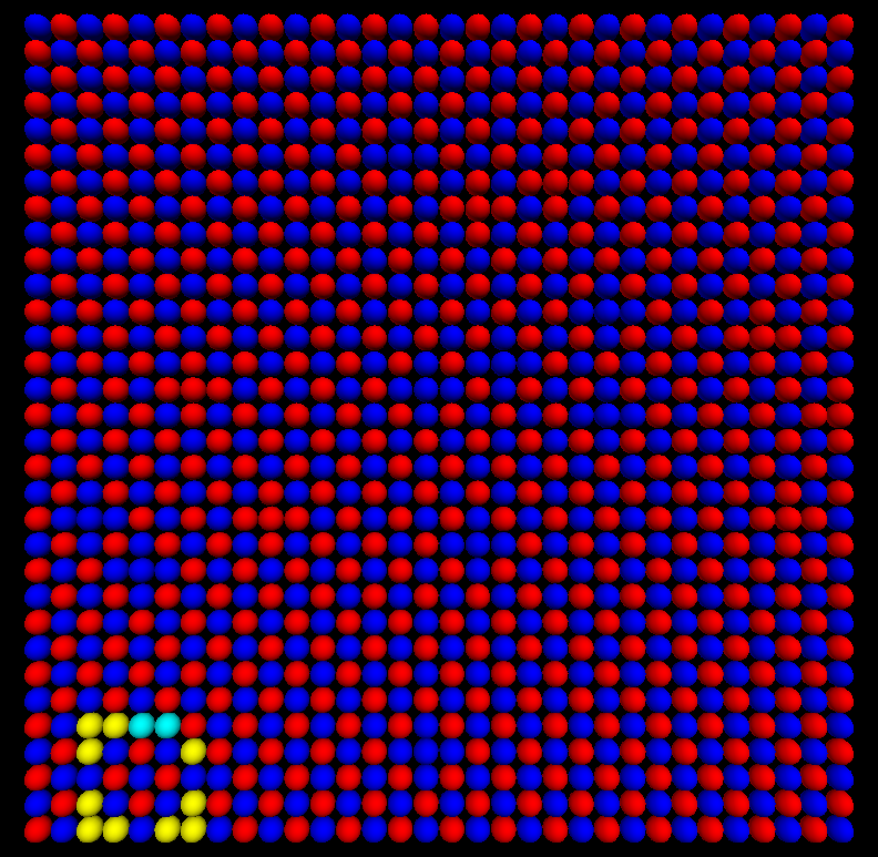
(c)

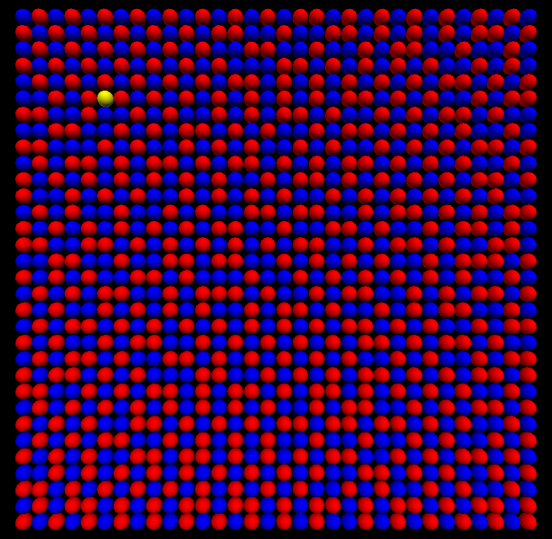
(d)

Figure 6: Examples of long-time configurations obtained for systems with $L=32$ under rules (a) 11000, (b) 11010, (c)11001, which give rise to anti-segregated patterns, and (d) under rule 11100, for which the final pattern resembles a tight sponge. Color code is the same as in Fig. 3.

Under rules 11000, 11010 and 11001, which correspond to the mirror rules of those yielding segregated states, the dynamics leads the system to a checkerboard 1x1 state with a small number of defects and a small average fraction of unsatisfied agents, which goes to zero in the thermodynamic limit. Figure 6 illustrates the long-time patterns, which can also be described as “anti-segregated”.

The energy function is of course positive, as illustrated in Fig. 2(a) for rule 11010. For the three rules we numerically obtain the long-time behavior $\rho_{u}\sim 1/L$, with a small corresponding survival probability; see Fig. 2(b) for rule 11010. The cusps seen in the curves are associated with the characteristic time needed for the survival probability to start decreasing from 100%, which grows with $L^{2}$. The small number of long-time configurations yielding blinkers is responsible for the asymptotic values of $\rho_{u}$ and $E$, which are calculated as the average of the corresponding values over the surviving simulations. Therefore, the cusps are a statistical feature rather than a behavior observable for a particular simulation.

For finite times and in the large $L$ regime, the fraction of unsatisfied agents decays roughly as $\rho_{u}\left(t\right)\sim 1/\sqrt{t}$ under the three rules, as for their mirror rules.

Sponge-like states

Rule	$E$	LTB	$\rho_{u}$
00111	nonincreasing	frozen	$\sim L^{-1}$
11100	nondecreasing	frozen	$\sim L^{-1}$
01111	nonincreasing	frozen	$\sim L^{-1}$
11110	nondecreasing	frozen	$\sim L^{-1}$
10111	nonincreasing	frozen	$\sim L^{-1}$
11101	nondecreasing	frozen	$\sim L^{-1}$
00110	oscillating	blinkers	$4.1\%$
01100	oscillating	blinkers	$4.1\%$
01110	oscillating	blinkers	$12\%$
01101	oscillating	mixed	$\sim L^{-1.2}$
10110	oscillating	mixed	$\sim L^{-1.5}$

Table 2: The 11 rules under which the long-time arrangement resembles a sponge, listing features of the energy function $E$, the long-time behavior (LTB) and the asymptotic dependence of the density $\rho_{u}$ of unsatisfied agents on the linear size $L$.

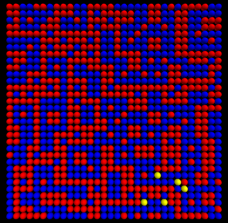
(a)

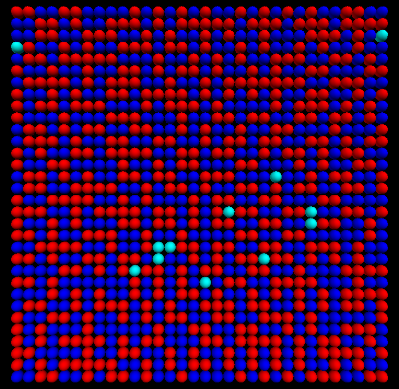
(b)

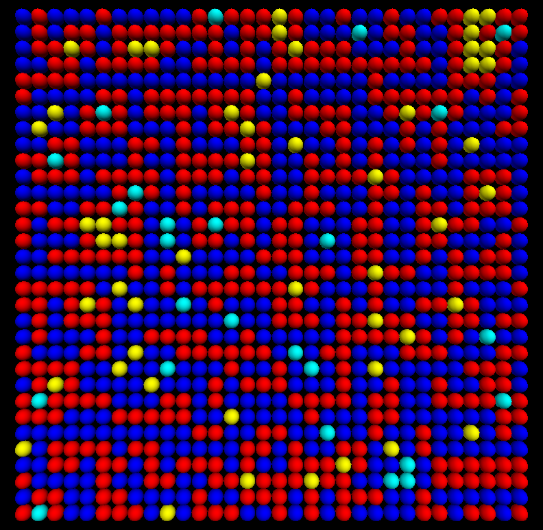
(c)

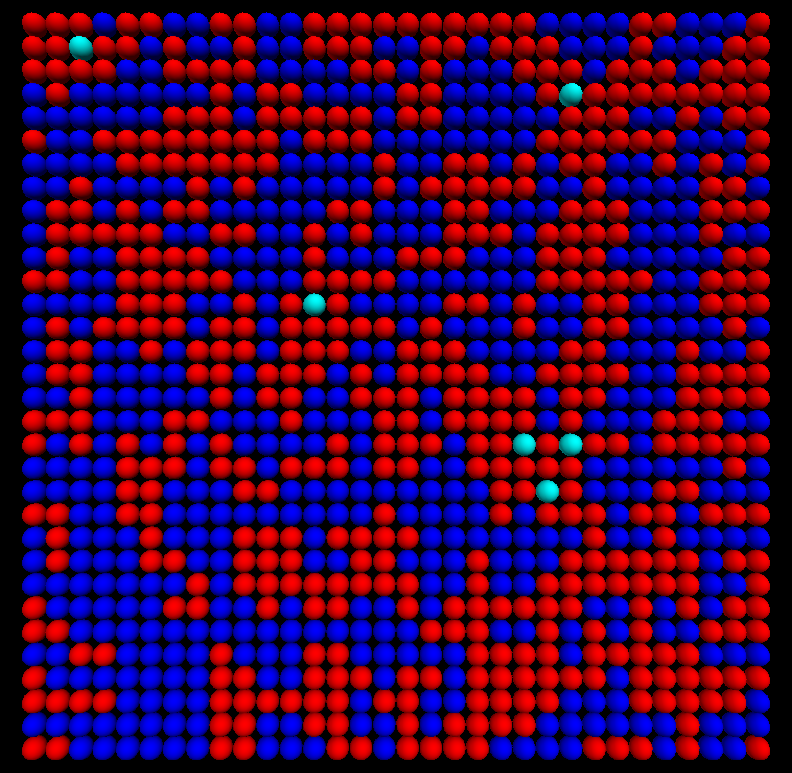
(d)

Figure 7: Examples of sponge-like patterns obtained for systems with $L=32$ under rules (a) 10110, (b) 01101, (c) 01110, (d) 01111. Color code is the same as in Fig. 3.

There are 11 rules under which the long-time behavior resembles a sponge pattern, and which are listed in Table 2. All of these rules have the striped pattern and either the checkerboard 1x2 or the double-striped patterns as fixed points, and the sponge-like long-time aspect can be attributed to the aggregation of domains of either vertical or horizontal dimers or stripes. Examples of the patterns are shown in Fig. 7.

Under six of these rules the dynamics always leads to a frozen arrangement, in which there are no unsatisfied agents of one type. This happens for rules (see Table 2) under which the energy cannot decrease or cannot increase, and the average fraction of unsatisfied agents upon freezing decreases as the inverse of the linear size $L$ of the system.

Under other rules (see Table 2), the long-time behavior is characterized by a small number of blinkers, whose density remains finite in the thermodynamic limit, with a survival probability of $100\%$. These are rules 01100 and 00110, related by a mirror transformation, as well as the result of their combination, rule 01110. Under rules 01100 and 00110, the fraction of unsatisfied agents decays to its asymptotic value after a characteristic time of order 200, exhibiting no $L$ dependence in the thermodynamic limit (see Fig. 2). On the other hand, under rule 01110 this decay happens after a time scale of order $L^{2}$, indicating that it cannot be reached in the thermodynamic limit. The average fraction $\rho_{u}=0.12$ indicated in Table 2 corresponds to the finite-time value, and is quite close to the mean-field value $\rho_{u}^{(\text{MF})}=0.125$ predicted by Eq. (4). The finite-time regime has no resemblance with a chaotic state, as one is able to show by calculating the average fraction of initially satisfied agents that ever become unsatisfied. This fraction also turns out to be around 0.12, so that most local configurations, such as those shown in Fig. 7(c), are static.

Finally, there are two rules (01101 and its mirror rule 10110) under which the long-time behavior strongly depends on the system size $L$. The dynamics may either lead to a frozen state or to a small fraction of blinkers, in both cases with a characteristic time corresponding to only one MC step. For $L$ below about $128$, the long-time survival probability (associated with the appearance of blinkers) is small, reaches a minimum value around $L=128$ and increases rapidly above $L$ around $256$, seeming to approach $100\%$ as $L\rightarrow\infty$. The long-time average fraction of unsatisfied agents seems to decrease with $L$ as a power law. We do not have an interpretation for this odd finite-size behavior at this time.

Rule 00111 corresponds to the von-Neumann neighborhood version of Schelling’s initial model, in which an agent is satisfied if at least half of its neighbors are of its same type. It yields a special type of sponge-like pattern, with rather broad “walls”. In this sense, it is quite close to the segregated pattern. For comparison, we show an example of the resulting patterns in Fig. 5(d).

Rule 11100, corresponding to the mirror-transformed version of rule 00111, produces patterns reminiscent of the anti-segregated patterns, despite the presence of small linear clusters of agents of the same type. For comparison, we show an example of the resulting patterns in Fig. 6(d).

3 Conclusions

In this paper we discussed an extension of Schelling’s model on a checkerboard, with no vacancies and the same number of agents of both types, in which for each number $n$ of same-type nearest neighbors we independently assign a binary satisfaction variable $s_{k}$ which is equal to one only if the agent is satisfied with that condition, and is equal to zero otherwise. Among the 32 resulting rules, 14 lead to a chaotic steady state, one does not evolve dynamically, 11 give rise to sponge-like patterns, while the remaining six rules lead to nearly perfect segregation, in which almost all agents are surrounded by agents of their same type, or to nearly perfect “anti-segregation”, in which almost all agents are surrounded by agents of the opposite type.

The three rules leading to nearly perfect segregation share the fact that agents are satisfied having either 3 or 4 neighbors of their same type. However, both the rule under which agents are also satisfied having only neighbors of the opposite type and the rule under which agents are satisfied having a single neighbor of their same type also lead to nearly perfect segregation. This is one more illustration of the robustness of segregation induced by a mild preference for a same-type neighborhood, already identified by Schelling.

The models studied here can be viewed as asynchronous cellular automata subject to constant “magnetization”, as we keep the total number of agents of each kind fixed. This is in contrast with models subject to the restriction of constant energy, as the Q2R automaton [26, 27], which provides an efficient way to simulate the square-lattice Ising model [28, 29]. The dynamical rule for this automaton prescribes that spins are flipped, one sublattice at a time, when they have two up and two down neighbors. This is similar to rule 11011, under which an agent is unsatisfied (and thus can move) only when it has exactly two neighbors of its same kind. Besides keeping the magnetization constant, the rule also differs from a fully asynchronous version of the Q2R automaton in that neighboring agents, therefore in different sublattices, can be switched in a single move, which incidentally leads to the increase of the energy function.

A natural question to ask is how the observations described here depend on the choice of neighborhood, on the assumption of an equal concentration of agents of each type, and on the choice of equal satisfaction parameters for both types of agents. We will provide an example of the effects of relaxing those restrictions in a future publication. As an illustration of the kind of behavior that appears, there occur transitions between active and inactive phases as the relative concentration of agents is varied, as in similar statistical-physics models [23, 24], such as the contact process and the voter model. This is of course related to the existence of absorbing states represented by the fixed points of the dynamics. Finally, another obvious extension of the present work would be to study synchronous versions of the various rules.

Appendix

Here we provide arguments pointing that, for any regular lattice, rules related by mirror transformation give rise to the same stationary density of unsatisfied agents, when there is the same number of agents of both types. We also discuss the relation between the average energy functions of a rule and of its mirror-transformed one, and derive Eq. (4).

Consider a regular lattice with coordination number $z$. Going beyond the mean-field approximation, we can write the stationary fractions of unsatisfied agents, $\rho_{u}\left(s\right)$, and of satisfied agents, $\rho_{s}\left(s\right)$, as

$$\rho_{u}\left(s\right)=\sum_{k=0}^{z}p_{k}\qquad\text{and}\qquad\rho_{s}\left(s\right)=\sum_{k=0}^{z}q_{k}$$

in which $p_{k}$ ($q_{k}$) is the steady-state probability that, under a given rule $s$, an unsatisfied (satisfied) agent has exactly $k$ agents of its opposite type.

Given a satisfaction rule defined by the parameter $s=s_{0}s_{1}s_{2}\cdots s_{z}$, the corresponding mirror rule is defined by $s^{\prime}=s_{0}^{\prime}s_{1}^{\prime}s_{2}^{\prime}\cdots s_{z}^{\prime}$, with $s_{k}^{\prime}=s_{z-k}$, and we represent by $p_{k}^{\prime}$ ($q_{k}^{\prime}$) the steady-state probability that, under rule $s^{\prime}$, an unsatisfied (satisfied) agent has exactly $k$ agents of its opposite type. For each neighborhood configuration of an unsatisfied agent of type $c$ containing $k$ agents of its opposite type under rule $s$, applying the mirror transformation to the neighboring agents generates a configuration containing $z-k$ agents of its opposite type which makes the agent unsatisfied under rule $s^{\prime}$. Since we assume an equal total number of agents of both types, and the dynamics only involves unsatisfied agents, we expect $p_{z-k}^{\prime}=p_{k}$. Therefore,

$$\rho_{u}\left(s^{\prime}\right)=\sum_{k^{\prime}=0}^{z}p_{k^{\prime}}^{\prime}=\sum_{k=0}^{z}p_{z-k}^{\prime}=\sum_{k=0}^{z}p_{k}=\rho_{u}\left(s\right).$$

so that rules related by mirror transformation should give rise to the same stationary density of unsatisfied agents, when there is the same number of agents of both types.

Although the last result also implies the equality of the fraction of satisfied agents under rules related by mirror transformation, $\rho_{s}\left(s^{\prime}\right)=\rho_{s}\left(s\right)$, which yields

$$\sum_{k=0}^{z}q_{k}=\sum_{k=0}^{z}q_{k}^{\prime},$$

we cannot automatically conclude that $q_{z-k}^{\prime}=q_{k}$, as that would imply the equivalence between each stable fixed point associated with $s$ and a stable fixed point associated with $s^{\prime}$. But in the square lattice, for instance, there is no equivalence between the checkerboard 1x1 pattern, in which each agent is surrounded by four agents of the opposite type, and the fully segregated pattern, which consists of two uniform domains separated by a boundary along which an agent necessarily has at least one neighbor of the opposite type. This is reflected in the fact that rule $11011$, which is mirror-symmetric, has a very small $q_{0}$ but a $q_{4}$ close to $1$, as shown by simulation results.

The average stationary energy per agent under rule $s$ is given by

$$\overline{E}\left(s\right)=\frac{1}{2}\sum_{k=0}^{z}E_{k}\left(p_{k}+q_{k}\right).$$

Under the mirror rule, we obtain

$$\overline{E}\left(s^{\prime}\right)=\frac{1}{2}\sum_{k^{\prime}=0}^{z}E_{k^{\prime}}\left(p_{k^{\prime}}^{\prime}+q_{k^{\prime}}^{\prime}\right)=\frac{1}{2}\sum_{k=0}^{z}E_{z-k}\left(p_{z-k}^{\prime}+q_{z-k}^{\prime}\right).$$

But $p_{z-k}^{\prime}=p_{k}$, and from the definition of the energy we have $E_{k}=-E_{z-k}$, so that

$$\overline{E}\left(s^{\prime}\right)=-\frac{1}{2}\sum_{k=0}^{z}E_{k}\left(p_{k}+q_{z-k}^{\prime}\right).$$

If we can assume that $q_{z-k}^{\prime}=q_{k}$, as in the cases in which there are no stable regular fixed points, then we can conclude that $\overline{E}\left(s^{\prime}\right)=-\overline{E}\left(s\right)$. This is what is numerically verified for 13 of the 14 rules in Table 1, but not for rule $11011$, under which checkerboard 1x1 domains outcompete the uniform domains in the long-time dynamics.

The mean-field approximation assumes that all local neighborhood configurations of an unsatisfied agent containing $k$ agents of its opposite type are equally probable, which is a reasonable assumption as long as there are no stable regular fixed points of the dynamics. Taking the number of agents of both types as equal, this leads to

$$p_{k}=\left(1-s_{k}\right)\frac{z!}{k!\left(z-k\right)!}\left(\frac{1}{2}\right)^{k}\left(\frac{1}{2}\right)^{z-k}=\left(\frac{1}{2}\right)^{z}\left(1-s_{k}\right)\frac{z!}{k!\left(z-k\right)!},$$

as in Eq. (4).

References

- [1] Thomas C Schelling 1969 Am. Econ. Rev. 59 488
- [2] Schelling T C 1971 J. Math. Soc. 1 143
- [3] Rogers T and McKane A J 2011 J. Stat. Mech.: Theory Exp. P07006
- [4] Henry A D, Prałat P and Zhang C Q 2011 Proc. Natl. Acad. Sci. U.S.A. 108 8605
- [5] Banos A 2012 Environment and Planning B: Planning and Design 39 393
- [6] Vinković D and Kirman A 2006 Proc. Natl. Acad. Sci. U.S.A. 103 19261
- [7] Stauffer D and Solomon S 2007 Eur. Phys. J. B 57 473
- [8] Dall’Asta L, Castellano C and Marsili M 2008 J. Stat. Mech.: Theory Exp. L07002
- [9] Gauvin L, Vannimenus J and Nadal J P 2009 The European Physical Journal B 70 293
- [10] Grauwin S, Bertin E, Lemoy R and Jensen P 2009 Proc. Natl. Acad. Sci. U.S.A. 106 20622
- [11] Gauvin L, Nadal J and Vannimenus J 2010 Phys. Rev. E 81 066120
- [12] Lemoy R, Berlin E and Jensen P 2011 EPL 93 38002
- [13] Goles Domic N, Goles E and Rica S 2011 Phys. Rev. E 83 056111
- [14] Rogers T and McKane A J 2012 Phys. Rev. E 85 041136
- [15] Albano E V 2012 J. Stat. Mech.: Theory Exp. P03013
- [16] Jensen P, Matreux T, Cambe J, Larralde H and Bertin E 2018 Phys. Rev. Lett. 120 208301
- [17] Ben-Naim E, Frachebourg L and Krapivsky P L 1996 Phys. Rev. E 53 3078
- [18] Sood V and Redner S 2005 Phys. Rev. Lett. 94 178701
- [19] Holme P and Newman M E J 2006 Phys. Rev. E 74 056108
- [20] Castellano C, Fortunato S and Loreto V 2009 Rev. Mod. Phys. 81 591
- [21] Teza G, Suweis S, Gherardi M, Maritan A and Cosentino Lagomarsino M 2019 Phys. Rev. E 99 032310
- [22] Durrett R and Zhang Y 2014 Proc. Natl. Acad. Sci. U.S.A. 111 14036
- [23] Marro J and Dickman R 1999 Nonequilibrium Phase Transitions in Lattice Models (Cambrige University Press)
- [24] Henkel M, Hinrichsen H and Lübeck S 2008 Nonequilibrium Phase Transitions Volume 1: Absorbing Phase Transitions (Springer)
- [25] Wolfram S 1983 Rev. Mod. Phys. 55 601
- [26] Vichniac G Y 1984 Physica D 10 96
- [27] Pomeau Y 1984 J. Phys. A: Math. Gen. 17 L415
- [28] Herrmann H J 1986 J. Stat. Phys. 45 145
- [29] Herrmann H J, Carmesin H O and Stauffer D 1987 J. Phys. A: Math. Gen. 20 4939