X-CIGALE: Fitting AGN/galaxy SEDs from X-ray to infrared

Abstract

CIGALE is a powerful multiwavelength spectral energy distribution (SED) fitting code for extragalactic studies. However, the current version of CIGALE is not able to fit X-ray data, which often provide unique insights into AGN intrinsic power. We develop a new X-ray module for CIGALE, allowing it to fit SEDs from the X-ray to infrared (IR). We also improve the AGN fitting of CIGALE from UV-to-IR wavelengths. We implement a modern clumpy two-phase torus model, SKIRTOR. To account for moderately extincted type 1 AGNs, we implement polar-dust extinction. We publicly release the source code (named “X-CIGALE”). We test X-CIGALE with X-ray detected AGNs in SDSS, COSMOS, and AKARI-NEP. The fitting quality (as indicated by reduced $\chi^{2}$) is good in general, indicating that X-CIGALE is capable of modelling the observed SED from X-ray to IR. We discuss constrainability and degeneracy of model parameters in the fitting of AKARI-NEP, for which excellent mid-IR photometric coverage is available. We also test fitting a sample of AKARI-NEP galaxies for which only X-ray upper limits are available from Chandra observations, and find that the upper limit can effectively constrain the AGN SED contribution for some systems. Finally, using X-CIGALE, we assess the ability of Athena to constrain the AGN activity in future extragalactic studies.

1 Introduction

Supermassive black holes (BHs) commonly exist in the centers of massive galaxies (e.g. kormendy95; kormendy13). BHs grow their mass ($M_{\rm BH}$) by accreting local material. During this process, a significant amount of the gravitational energy of the accreted material is converted to radiation, and the system shines as an active galactic nucleus (AGN). The typical spectral energy distribution (SED) of AGNs covers a broad wavelength range, from X-ray to infrared (IR).

AGN emission at different wavelengths is generated by different physical processes (e.g. netzer13). The accretion disk mostly produces photons at ultraviolet (UV) and optical wavelengths. Some of these photons are scattered to X-ray energies by the hot corona above the disk (i.e. inverse Compton scattering). Some of the UV/optical photons might also be absorbed by dust. The dust is thus heated and reemits the energy as infrared radiation. Considering the tight link between AGN multiwavelength SEDs and these physical processes, it is feasible to infer source properties from modelling the observed photometric data. On the other hand, the observed SED is often complicated, involving factors such as host-galaxy contributions and dust extinction. Misinterpretation of the SED could lead to unrealistic physical properties. Therefore, it is critical to decipher the observed data appropriately with a powerful and reliable SED fitting code.

The Code Investigating GALaxy Emission (CIGALE) is a state-of-the-art python code for SED fitting of extragalactic sources (boquien19). It employs physical AGN and galaxy models, and allows flexible combination between them. The current version of CIGALE can simultaneously fit the observed SED from UV to far-IR (FIR) and extract source physical properties such as AGN luminosity and host stellar mass ($M_{\star}$). However, the current CIGALE is not able to model X-ray fluxes, which often provide a unique view of AGNs.

X-ray observations have many advantages in AGN studies (see brandt15 for a review). Strong X-ray emission is nearly a universal property of the AGN phenomenon. X-rays are generated from the immediate vicinity of the BH, directly revealing the intrinsic AGN power. Therefore, X-ray fluxes are widely used as a tracer of BH accretion rate (e.g. yang18; yang19). Thanks to their great penetrating power, X-rays are only mildly affected by obscuration in general. Also, AGNs are much more efficient in generating X-rays than their host galaxies. Therefore, the observed X-ray fluxes are often dominated by AGNs and have negligible galaxy contribution. Considering these advantageous properties, X-ray observations are widely used to select AGNs, especially in the distant universe, (e.g. luo17; chen18). These selections are often more complete and reliable than the selections at other wavelengths such as optical and IR.

Besides the lack of X-ray fitting capability, CIGALE’s current AGN model (fritz06), which covers the UV to IR, also has some other disadvantages. The model assumes that the central engine is surrounded by a dusty torus (i.e. the AGN unified model; antonucci93; urry95; netzer15; zou19). The torus absorbs a fraction of the UV and optical emission from the central engine and reemits the energy as IR photons. When viewing from the equatorial direction, the central engine is obscured and only reemitted IR radiation can be observed (type 2 AGN). When viewing from the polar direction, the central engine is directly visible (type 1 AGN).

One disadvantage of the AGN model is that it assumes the dusty torus is a smooth structure. However, such smooth models for the torus are disfavored on physical grounds (e.g. tanimoto19). To reach a scale height consistent with observations, the dust grains in a smooth torus would have random velocities $\sim 100$ km s${}^{-1}$, corresponding to a temperature of $\sim 10^{6}$ K. This high temperature far exceeds the dust-sublimation temperature ($\sim 10^{3}$ K). Another disadvantage of the AGN model is that the disk emission is assumed to be absolutely unextincted for the case of type 1. However, recent observations indicate that a non-negligible amount of extinction exists for some type 1 AGNs (e.g. bongiorno12; elvis12; lusso12), which can be attributed to the dust existing along polar directions (e.g. stalevski17; stalevski19; lyu18). The current CIGALE cannot model the SEDs of these type 1 AGNs.

In this paper, we further develop CIGALE and enable it to fit X-ray data. The new development allows CIGALE to model AGN SED from X-ray to IR simultaneously and extract source properties such as AGN intrinsic luminosity and host-galaxy stellar mass ($M_{\star}$). Besides developing the X-ray part, we also improve CIGALE’s capability in fitting the UV-to-IR SED of AGNs. We implement the latest version of SKIRTOR, a clumpy two-phase torus model derived from a modern radiative-transfer method (stalevski12; stalevski16). In addition, we introduce polar-dust extinction to account for the possible extinction in type 1 AGNs. We name the new version of CIGALE as “X-CIGALE”.

The structure of this paper is as follows. In §2, we outline the scheme of our new code development. In §3, we test X-CIGALE on AGNs with X-ray detections from different surveys. We test fitting galaxies with only X-ray upper limits in §LABEL:sec:uplim. We summarize our results and discuss future prospects in §LABEL:sec:sum.

Throughout this paper, we assume a flat $\Lambda$CDM cosmology with $H_{0}=69.3$ km s${}^{-1}$ Mpc${}^{-1}$ and $\Omega_{M}=0.286$ (WMAP 9-year results; hinshaw13). Quoted uncertainties are at the $1\sigma$ (68%) confidence level, unless otherwise stated. Quoted optical/infrared magnitudes are AB magnitudes.

2 The code

We briefly summarize the mechanisms and features of CIGALE in §2.1. In §2.2, §2.3, and §2.4, we detail our new development of X-CIGALE, i.e. the X-ray fitting, SKIRTOR, and the polar-dust extinction. The new inputs/outputs introduced in X-CIGALE are listed in Appendix LABEL:sec:in_and_out.

2.1 A brief introduction of CIGALE

CIGALE is an efficient SED-fitting code which has been developed for more than a decade (burgarella05; noll09; serra11; boquien19). CIGALE is written in Python. X-CIGALE is built upon CIGALE, and the fitting algorithm of X-CIGALE is the same as that of CIGALE. Here, we only briefly introduce the algorithm, and interested readers should refer to boquien19 for a detailed description.

CIGALE allows the user to input a set of model parameters. The code then realizes the model SED for each possible combination of the model parameters, and convolves the model SED with the filters to derive model fluxes. By comparing the model fluxes with the observed fluxes, the code computes likelihood as $L=\exp(-\chi^{2}/2)$ for each model. CIGALE supports two types of analyses, i.e. maximum likelihood (minimum $\chi^{2}$) and Bayesian-like. In the maximum-likelihood analyses, CIGALE picks out the model with the largest $L$ value, and calculates physical properties such as $M_{\star}$ and star formation rate (SFR) from this single model. In the Bayesian-like analyses, for each physical property, CIGALE calculates the marginalized probability distribution function (PDF) based on the $L$ values of all models. Finally, from this PDF, CIGALE derives the probability-weighted mean and standard deviation, and outputs them as the estimated value and uncertainty.

Among the above processes, one key step is the realization of model SEDs from input parameters. This procedure relies on a set of modules, and each module is responsible for a function that shapes the SED. For example, the “nebular emission” module adds the nebular-emission components to the SED, and the “dust attenuation” module extincts the SED. Our new development of X-CIGALE follows this module-based structure. We enable CIGALE to fit X-ray data by developing a new X-ray module (§2.2); we implement SKIRTOR templates and polar-dust extinction in a new SKIRTOR module (§2.3 and §2.4).

2.2 The new X-ray module

In this section, we develop a new X-ray module to enable X-CIGALE to fit X-ray data. In §2.2.1, we detail the basic settings of this new module. In §2.2.2, we present the adopted X-ray SED for AGN and galaxy components. In §2.2.3, we present the relation that we used to link AGN X-ray with other wavelengths. We note that our new developments are for the majority AGN population in optical/X-ray surveys, and thus X-CIGALE may not be applicable to some minor populations such as radio-loud and broad absorption line (BAL) objects (e.g. brandt00; miller11). We leave the treatment of these particular AGNs to future works.

2.2.1 Basic settings

As presented in §1, the X-ray band has many advantages in studying AGNs. Therefore, we implement an X-ray module for X-CIGALE. The main goal of this module is to connect X-ray with other wavelengths, rather than to obtain detailed X-ray spectral properties (e.g. photon index and hydrogen column density) by performing detailed X-ray spectral analyses. This is because the latter has already been well realized by many specialized X-ray codes such as XSPEC (arnaud96) and Sherpa (freeman01), and there is no need for X-CIGALE to perform similar analyses. Also, it is technically difficult to fit the X-ray spectra within the framework of X-CIGALE. X-CIGALE assumes that a sample of sources are observed with a single “filter transmission”, as is the case in UV-to-IR data. However, at X-ray wavelengths, the transmission curve varies from source-to-source, as it might depend on many factors such as position on the detectors and observation date. For example, the soft-band transmission of Chandra has been continuously declining since its launch (e.g. odell17). In fact, each source is associated with a unique transmission curve and the curve is taken into account when fitting the X-ray spectra with, e.g. XSPEC and Sherpa.

Therefore, the X-ray module of X-CIGALE is designed to work on the high-level X-ray data products, i.e. intrinsic X-ray fluxes in a given band. We require the X-ray fluxes to be corrected for telescope transmission. Fortunately, this correction is embedded in routine X-ray data processing and has already been applied in X-ray photometric catalogs (e.g. yang16; luo17). Since the transmission has already been considered, X-CIGALE only needs to adopt a uniform-sensitivity (i.e. boxcar-shaped) “filter”. We have already included a few typical boxcar X-ray filters, e.g. 0.5–2 keV and 2–7 keV for convenience, while the user can easily generate the filters for any X-ray band.

In addition, we require the input X-ray fluxes to be “absorption-corrected”. The absorption might be from the source itself, our Galaxy, and/or the intergalactic medium (IGM; e.g. starling13). However, we do not differentiate these types of absorption, as it is often infeasible to separate them in X-ray data analyses. The absorption correction can be obtained from routine X-ray data processing, e.g., spectral analyses via XSPEC/Sherpa or band-ratio analyses (e.g. xue16; luo17). The user may also choose to use hard X-ray bands where absorption corrections are generally small (e.g. yang18; yang18b).

In X-ray catalogs (e.g. xue16; luo17), X-ray fluxes ($f_{\rm X}$) are conventionally given in the cgs units of erg s${}^{-1}$ cm${}^{-2}$, but X-CIGALE requires the input fluxes ($f_{\rm cigale}$) to be given in the units of mJy. Therefore, the user needs to convert the flux units with

$$f_{\rm cigale}=\frac{f_{\rm x}\times 4.136\times 10^{8}}{E_{\rm up}-E_{\rm lo}}$$ (1)

where $E_{\rm lo}$ and $E_{\rm up}$ refer to the lower and upper limits of the energy band in units of keV.

The X-ray module covers rest-frame $10^{-3}$–5 nm, corresponding to $\approx$ 0.25–1200 keV. Such an energy range is sufficient for practical purposes: current X-ray instruments cannot observe energies significantly below rest-frame $0.5(1+z)$ keV in general; the AGN flux is typically non-detectable above $\approx 1000$ keV due to the existence of the cut-off energy in AGN X-ray spectra (see §2.2.2).

2.2.2 X-ray SED

To first-order approximation, the intrinsic AGN X-ray spectrum is typically a power law with a high-energy exponential cutoff, i.e.

$$f_{\nu}\propto E^{-\Gamma+1}\exp(-E/E_{\rm cut})$$ (2)

where $\Gamma$ is the so-called “photon index”, widely adopted in X-ray astronomy, and $E_{\rm cut}$ is the cutoff energy. We adopt this spectral shape in X-CIGALE. Detailed X-ray spectral fitting in the literature finds $\Gamma\approx 1.8$ (e.g. yang16; liu17). We allow the user to set $\Gamma$ in X-CIGALE. We set $E_{\rm cut}=300$ keV, the typical value from the observations of Seyferts (e.g. dadina08; ricci17). Note that since $E_{\rm cut}$ is above the highest observable energy of most X-ray observatories (e.g. Chandra and XMM-Newton), the exact choice of $E_{\rm cut}$ has practically negligible effects on the fitting with X-CIGALE for most cases. The adopted AGN X-ray SED is displayed in Fig. 1.

Besides AGNs, galaxies can also emit X-rays, although the emission from galaxies is often much weaker than that from AGNs for X-ray detected sources. There are three main origins of galaxy X-ray emission: low-mass X-ray binaries (LMXB), high-mass X-ray binaries (HMXB), and hot gas. The strengths of these components can be modeled as a function of galaxy properties such as $M_{\star}$ and SFR. We adopt the recipe from mezcua18, where a chabrier03 initial mass function (IMF) is assumed. In this scheme, the LMXB and HMXB luminosities (in units of erg s${}^{-1}$) are described as

$$\begin{split}\log(L_{\rm 2-10\ keV}^{\rm LMXB}/M_{\star})=40.3-1.5\log t-0.42(\log t)^{2}+\\ 0.43(\log t)^{3}+0.14(\log t)^{4}\\ \log(L_{\rm 2-10\ keV}^{\rm HMXB}/{\rm SFR})=40.3-62Z+569Z^{2}-1834Z^{3}+1968Z^{4}\end{split}$$ (3)

where $M_{\star}$ and SFR are in solar units; $t$ denotes stellar age in units of Gyr; $Z$ denotes metallicity (mass fraction). The hot-gas luminosity (in units of erg s${}^{-1}$) is described as

$$\log(L_{\rm 0.5-2keV}^{\rm hotgas}/{\rm SFR})=38.9$$ (4)

Similarly as for AGN, we also employ the SED shape in Eq. 2 for all three components, with $E_{\rm cut}$ fixed at 100 keV (LMXB and HMXB; e.g. zhang97; motta09) and 1 keV (hot gas; e.g. mathews03). We allow the user to set $\Gamma$ values for the LMXB and HMXB components. In our test fitting in §3, we set $\Gamma$ to 1.56 and 2.0 for LMXB and HMXB, respectively (e.g. fabbiano06; sazonov17). Adjusting these $\Gamma$ does not affect the fitting results significantly, as the observed X-ray fluxes are often dominantly contributed by AGNs rather than galaxies. The X-ray continuum from hot gas can be modelled as free-free and free-bound emission from optically thin plasma ($\Gamma=1$; e.g. mewe86). Therefore, we fix $\Gamma=1$ for the hot-gas component in X-CIGALE. Fig. 1 shows the adopted X-ray SEDs of the three components. We add all three components for the total X-ray SED from galaxies.

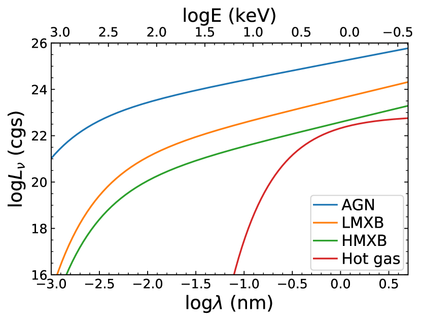
Figure 1: An example X-ray SED model for a typical source with AGN $L_{\rm 2\text{--}10\ keV}=10^{43}$ erg s${}^{-1}$, $M_{\star}=10^{11}$ $M_{\odot}$, ${\rm SFR}=10\ M_{\odot}$ yr${}^{-1}$, $T=1$ Gyr, and $Z=0.02$. Different colors indicate different components. For this source, the X-ray luminosity is dominantly contributed by the AGN.

2.2.3 The $\alpha_{\rm ox}$-$L_{2500\textup{\AA}}$ relation

As in §2.2.1, the main goal of X-CIGALE is to fit X-ray and other wavelengths simultaneously. Some known connections between X-ray and other wavelengths must be applied; otherwise, the fitting would be practically useless. We adopt the well-studied “$\alpha_{\rm ox}$-$L_{2500\textup{\AA}}$” relation (e.g. steffen06; just07; lusso17), where $L_{2500\textup{\AA}}$ is AGN intrinsic (de-reddened) luminosity per frequency at 2500 Å and $\alpha_{\rm ox}$ is the SED slope between UV (2500 Å) and X-ray (2 keV), i.e.

$$\alpha_{\rm ox}=-0.3838\log(L_{2500\textup{\AA}}/L_{\rm 2keV}).$$ (5)

The observed $\alpha_{\rm ox}$-$L_{2500\textup{\AA}}$ relation (just07) is written as

$$\alpha_{\rm ox}=-0.137\log(L_{2500\textup{\AA}})+2.638$$ (6)

where $L_{2500\textup{\AA}}$ is in units of erg s${}^{-1}$ Hz${}^{-1}$. The 1$\sigma$ intrinsic dispersion of this $\alpha_{\rm ox}$-$L_{2500\textup{\AA}}$ relation is $\Delta\alpha_{\rm ox}\approx 0.1$ (see Table 8 of just07). Here, $\Delta\alpha_{\rm ox}$ is the $\alpha_{\rm ox}$ deviation from that expected from the $\alpha_{\rm ox}$-$L_{2500\textup{\AA}}$ relation, i.e.

$$\Delta\alpha_{\rm ox}=\alpha_{\rm ox}-\alpha_{\rm ox}(L_{2500\textup{\AA}}).$$ (7)

Observations have found that the $\alpha_{\rm ox}$-$L_{2500\textup{\AA}}$ relation does not have significant redshift evolution, indicating that the relation originates from fundamental accretion physics (steffen06; just07; lusso17). We allow the user to set the maximum $|\Delta\alpha_{\rm ox}|$ allowed ($|\Delta\alpha_{\rm ox}|_{\rm max}$). Internally, X-CIGALE calculates all models with $\alpha_{\rm ox}$ from $-1.9$ to $-1.1$ with a step of 0.1. X-CIGALE then calculates $|\Delta\alpha_{\rm ox}|$ and discards the models with $|\Delta\alpha_{\rm ox}|>|\Delta\alpha_{\rm ox}|_{\rm max}$. In our test fitting (§3 and §LABEL:sec:uplim), we adopt $|\Delta\alpha_{\rm ox}|_{\rm max}=0.2$, corresponding to the $\approx 2\sigma$ scatter of the $\alpha_{\rm ox}$-$L_{2500\textup{\AA}}$ relation (just07).

Note that the $\alpha_{\rm ox}$-$L_{2500\textup{\AA}}$ relation above is derived from observations, assuming that the unobscured AGN emission is isotropic at both UV/optical and X-ray wavelengths. However, the UV/optical emission is unlikely isotropic, because it is from the accretion disk and the effects of projected area and limb darkening affect the angular distribution of the radiative energy. After considering these effects, the disk luminosity can be approximated as $L(\theta)\propto\cos\theta(1+2\cos\theta)$, where $\theta$ is the angle from the AGN axis (e.g. netzer87). This angular dependence of disk emission is adopted in SKIRTOR, the UV-to-IR AGN module adopted in X-CIGALE (see §2.3). The X-ray emission should likely be less anisotropic than the UV/optical emission, because the X-rays originate from re-processed UV/optical photons via inverse Compton scattering. However, the exact relation between X-ray flux and viewing angle depends on model details, such as corona shape and opacity, which are poorly known (e.g. liu14; xu_y15). For simplicity, we assume that the X-ray emission is isotropic.

Our assumption of anisotropic UV/optical emission and isotropic X-ray emission leads to a dependence of $\alpha_{\rm ox}$-$L_{2500\textup{\AA}}$ on viewing angle. We further assume that the observed $\alpha_{\rm ox}$-$L_{2500\textup{\AA}}$ relation for type 1 AGNs reflects the intrinsic $\alpha_{\rm ox}$-$L_{2500\textup{\AA}}$ relation for all AGNs at a “typical” viewing angle of $\theta=30^{\circ}$. This value approximates the probability-weighted viewing angle for type 1 AGNs, i.e.

$$\theta\approx\frac{\int_{0}^{90^{\circ}-\Delta}\theta\sin\theta d\theta}{\int_{0}^{90^{\circ}-\Delta}\sin\theta d\theta}\approx 30^{\circ},$$ (8)

where $\Delta$ denotes the angle between the equatorial plane and edge of the torus, i.e., half opening angle. The typical value is $\Delta\approx 40^{\circ}$ from observations (e.g. stalevski16). Although $\Delta$ is a free parameter in X-CIGALE, we do not recommend the user choose other values than $40^{\circ}$, as this value is favored by observations and is consistently adopted throughout the build-up of the X-CIGALE code. The weight $\sin\theta$ is proportional to the probability for the viewing angle being $\theta$.

We note that our SED fitting results (§3 and §LABEL:sec:uplim) are not sensitive to the assumed typical $\theta$, and will not change significantly if adjusting $\theta$ within the range of $\approx 10^{\circ}$–$50^{\circ}$. In the X-CIGALE output (Appendix LABEL:sec:in_and_out), the $\alpha_{\rm ox}$ and $L_{2500\textup{\AA}}$ always refer to the value at $\theta=30^{\circ}$, regardless of the actual viewing angle in the model. This $\alpha_{\rm ox}$ and $L_{2500\textup{\AA}}$ design is to reflect AGN essential properties, independent of the viewing angle. By changing the integral ranges in Eq. 8 to $(90^{\circ}-\Delta,90^{\circ})$, we can derive the probability-weighted $\theta$ for type 2 AGNs, i.e. $\theta\approx 70^{\circ}$. These typical $\theta$ values (type 1: $\approx 30^{\circ}$, type 2:$\approx 70^{\circ}$) are used in our SED fitting (§3 and §LABEL:sec:uplim).

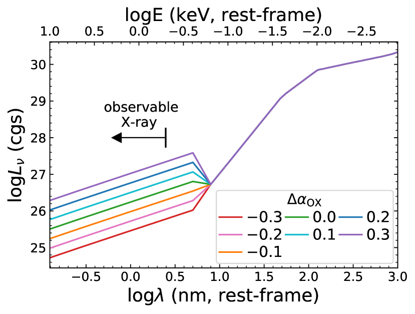
Figure 2: The model SEDs for an unobscured AGN with $\log L_{2500\textup{\AA}}=30$ (cgs). Different colors indicate different $\alpha_{\rm ox}$. The “breaks” at $5$ nm are caused by the wavelength limit of the X-ray module, which ends at 5 nm. As explained in §2.2.3, such breaks are generally not problematic for practical purposes, as most X-ray instruments only cover wavelengths $\lesssim 10^{0.4}$ nm ($\gtrsim 0.5$ keV, as marked).

2.3 SKIRTOR

The previous CIGALE AGN model responsible for the UV-to-IR SED is from fritz06. This model assumes that the dusty torus is a smooth structure. However, more recent theoretical and observational works find that the torus is mainly made of dusty clumps (e.g. nikutta09; ichikawa12; stalevski12; tanimoto19). SKIRTOR is a clumpy two-phase torus model (stalevski12; stalevski16), based on the 3D radiative-transfer code, SKIRT (baes11; camps15). In SKIRTOR, most (mass fraction $=97\%$) of the dust is in the form of high-density clumps, while the rest is smoothly distributed. In addition, SKIRTOR considers the anisotropy of the power source, AGN disk emission (see §2.2.3), while Fritz’s model simply assumes isotropic disk emission. Therefore, we implement SKIRTOR within X-CIGALE. We recommend using SKIRTOR as the UV-to-IR SED model of AGNs, although X-CIGALE allows the user to choose between SKIRTOR and Fritz’s model.

SKIRTOR adopts a disk SED that has a higher fraction of far-UV luminosity ($\lesssim 100$ nm) compared to observations (see §3.2.1 of duras17). Following duras17, we update SKIRTOR with a new disk SED (feltre12) that is supported by observations, i.e.

$$\lambda L_{\lambda}\propto\begin{cases}\lambda^{2}&\qquad 8\leq\lambda<50\ [\mathrm{nm}]\\ \lambda^{0.8}&\qquad 50\leq\lambda<125\ [\mathrm{nm}]\\ \lambda^{-0.5}&\qquad 125\leq\lambda<10^{4}\ [\mathrm{nm}]\\ \lambda^{-3}&\qquad\lambda>10^{4}\ [\mathrm{nm}].\end{cases}$$ (9)

We modify the disk SED with the following method. We denote the old and new intrinsic disk SEDs as $L^{\rm old}_{\lambda,\rm normed}$ and $L^{\rm new}_{\lambda,\rm normed}$, respectively, where the subscript “normed” indicates the total power of these SEDs has been normalized to unity. Then the new observed disk SED component (which might be obscured) can be converted from the old one by multiplying by the factor, $L^{\rm new}_{\lambda,\rm normed}/L^{\rm old}_{\lambda,\rm normed}$. The new scatter component can be obtained in the same way; the dust reemitted component remains unchanged. The method above keeps energy balance. This method is also described on the SKIRTOR official webpage.

2.4 Polar Dust

2.4.1 The extinction of type 1 AGN

In SKIRTOR (also in Fritz’s model), the extinction of UV and optical radiation for type 1 AGN is assumed to be negligible. This assumption holds for most optically selected blue quasars. For example, richards03 found only $\approx 6\%$ of their SDSS quasars are extincted. However, the assumption might not be true for, e.g. X-ray selected AGNs. For example, in the COSMOS AGN catalogs selected by XMM-Newton (bongiorno12), the fraction of extincted sources ($E(B-V)\geq 0.1$) among broad-line AGNs is $\approx 40\%$.

To check the extinction of type 1 AGNs, we compare the median UV-optical SEDs of spectroscopically classified type 1 AGNs in SDSS and COSMOS (see §3 for details). These median SEDs are derived from the photometric data in §3. For each source in a sample, we interpolate the observed photometry to obtain $F_{\nu}$ as a function of observed-frame wavelength. We then shift this interpolated SED to rest-frame wavelength and normalize $F_{\nu}$ at 250 nm. Finally, at each wavelength, we obtain the median $F_{\nu}$ of all the sources in the sample. Fig. 3 (left) shows the results. The SDSS median SED is similar to the typical unobscured quasar SED of $F_{\nu}\propto\lambda^{0.5}$ (see Eq. 9). In contrast, the COSMOS median SED is significantly redder than $F_{\nu}\propto\lambda^{0.5}$ (e.g. elvis12). We note that this difference in SED shape is observationally driven by selection effects. The SDSS sample consists of optically selected, and is thus biased toward blue and optically bright objects. The COSMOS sample consists of X-ray selected objects and does not suffer from significant bias in the UV/optical (e.g. brandt15). Although driven by selection effects, Fig. 3 (left) at least indicates that reddened AGN SEDs indeed exist, and we discuss the physical cause of the SED reddening below.

The red SED shape might be physically caused by the aforementioned dust extinction. However, another potential physical cause is host-galaxy contribution to the SED. Since the UV/optical SEDs of galaxies are generally redder than those of unobscured AGNs (e.g. Fig. 3 of salvato09), AGN-galaxy mixed SEDs tend to be redder than pure AGN SEDs. To investigate the cause of SED reddening, we can compare the magnitudes that sample rest-frame UV wavelengths for COSMOS and SDSS, as galaxy contributions to the photometry should be small at UV wavelengths. In Fig. 3 (right), we show the $r$-band (rest-frame $\lesssim 2000\ \textup{\AA}$) magnitude distributions at $z=2-2.5$ and $f_{\nu,\rm 2keV}=3\text{--}10$ ($10^{-7}\ \rm mJy$, the results are similar for other redshift/X-ray flux bins). The control of redshift and X-ray flux is to force the compared samples to have similar X-ray luminosities and thereby bolometric luminosities (assuming the X-ray bolometric correction factors are similar for the sources). The COSMOS AGNs are systematically fainter than the SDSS AGNs in UV/optical. Therefore, Fig. 3 (right) indicates that, at a given AGN bolometric luminosity, the rest-frame UV AGN luminosities of COSMOS are typically lower than those of SDSS, supporting the existence of dust extinction. We conclude that dust extinction is at least one of the physical causes of the SED reddening (Fig. 3 left), although galaxy SED contributions might enhance the reddening (e.g. bongiorno12).

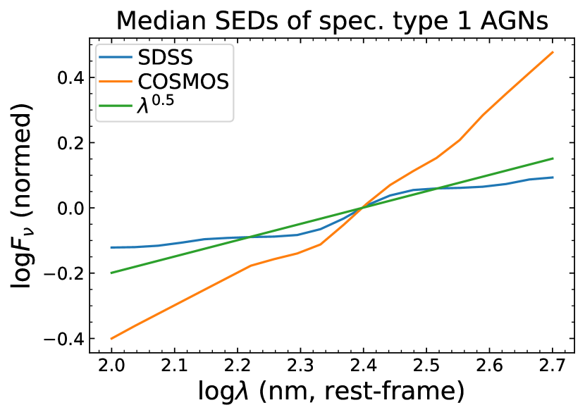
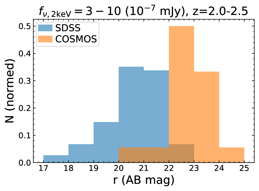
Figure 3: Left: Median SEDs of spectroscopic type 1 AGNs in SDSS (blue, optically selected) and COSMOS (orange, X-ray selected). The green curve shows a typical unobscured quasar SED. All the SEDs are normalized at 250 nm. The SDSS SED is similar to the typical quasar SED. The COSMOS SED is significantly redder than the SDSS SED, indicating the presence of dust extinction and/or host-galaxy contribution for the COSMOS sources. Right: The observed $r$-band magnitude distributions for SDSS and COSMOS type 1 AGNs. Both AGN samples are in the bins of $z=2\text{--}2.5$ and $f_{\nu,\rm 2keV}=3\text{--}10\ (10^{-7}\ \rm mJy)$. The SDSS AGNs are systematically brighter than the COSMOS AGNs, and this qualitative result also holds for other redshift/X-ray flux bins. This result indicates that dust extinction should be at least one of the causes for the red SED shapes of the COSMOS AGNs, although galaxy SED contributions might enhance the reddening. This figure does not compare the AKARI-NEP sample in §LABEL:sec:akari, because spectroscopic identifications of type 1 AGNs are not available for AKARI-NEP (§LABEL:sec:sample_akari).

2.4.2 The polar-dust model

From §2.4.1, it is necessary to account for dust extinction of type 1 AGNs in X-CIGALE. The geometry of the obscuring materials is sketched in Fig. 4, where the materials responsible for type 1 AGN obscuration are called “polar dust” (e.g. lyu18). The existence of polar dust has been proved by high-resolution mid-IR (MIR) imaging of local Seyfert galaxies (e.g. lopez_gonzaga14; stalevski17; stalevski19; asmus19). However, the physical properties of the polar dust could be complicated and vary for different objects. For example, it might be close to the dust-sublimation radius ($\sim$ pc scale; e.g. lyu18) or on galactic scales ($\sim$ kpc; e.g. zou19).

Considering these complexities, we do not build a grid of physical models and perform radiation-transfer simulations. Instead, we employ several empirical extinction curves, including those from calzetti00, gaskell04, and prevot84, and the user can choose among these curves. In our tests of X-CIGALE (§3 and §LABEL:sec:uplim), we adopt the SMC extinction curve, which is preferred from AGN observations (e.g. hopkins04b; salvato09; bongiorno12; but also see, e.g. gaskell04). The extinction amplitude (parameterized as $E(B-V)$) is a free parameter set by the user, and setting $E(B-V)=0$ returns to the original torus.

Since the scheme of X-CIGALE maintains energy conservation, we need to implement dust emission to account for the radiative energy absorbed by the dust. We assume the dust reemission is isotropic. For simplicity, we adopt the “grey body” model (e.g. casey12), i.e.

$$L_{\nu}(\lambda)\propto\frac{\left(1-\mathrm{e}^{-\left(\lambda_{0}/\lambda\right)^{\beta}}\right)\left(\frac{c}{\lambda}\right)^{3}}{\mathrm{e}^{hc/\lambda kT}-1},$$ (10)

where $\lambda_{0}$ is fixed at 200 $\mu$m, emissivity ($\beta$) and temperature ($T$) are free parameters set by the user. $L_{\nu}$ in Eq. 10 is normalized so that total energy is conserved, i.e.

$$L^{\rm emit}_{\rm total}=\int_{0}^{90^{\circ}-\Delta}L^{\rm extinct}_{\rm total}(\theta)\sin\theta d\theta$$ (11)

where $L_{\rm total}^{\rm emit}$ is the dust reemitted luminosity (angle-independent) and $L^{\rm extinct}_{\rm total}$ is the luminosity loss caused by polar-dust extinction (angle-dependent). Note that the integral on the right-hand-side of Eq. 11 is to account for the fact that the polar dust only accounts for the obscuration in the polar directions while the polar-dust reemission is in all directions (see Fig. 4; e.g. Eq. 8). Fig. 5 shows the model SEDs for different extinction levels, where $T=100$ K, $\beta=1.6$, and $\Delta=40^{\circ}$.

Our model above follows the AGN-unification scheme, i.e. AGN type is determined solely by the viewing angle, which is a free parameter in X-CIGALE. When the viewing angle is within the polar directions (type 1), the observed AGN disk emission suffers moderate (or none if $E(B-V)=0$) extinction from the polar dust. When the viewing angle is within the equatorial directions (type 2), the observed AGN disk emission is strongly obscured by the torus. If the AGN type is known (e.g. from spectroscopy), the user can limit the viewing angle to the polar or equatorial direction (§3.1 and §3.2). Otherwise, the user can adopt multiple viewing angles including both polar and equatorial directions, and let X-CIGALE choose freely between them (§LABEL:sec:akari). For example, if the user set “viewing angles = 30${}^{\circ}$, 70${}^{\circ}$; $E(B-V)=0.1$”, then CIGALE will build two model SEDs. For the 30${}^{\circ}$ model (type 1), the UV/optical SED is reddened by the $E(B-V)=0.1$ polar dust whose reemission also contributed to the IR SED. For the 70${}^{\circ}$ model (type 2), the polar dust does not affect the UV/optical SED (already obscured by torus), but its reemission still contributes to the IR SED.

Our polar-dust model above provides one possible scenario for the reddened type 1 AGNs, i.e. the viewing angle is small and the extinction is caused by dust along the polar directions. An alternative scenario is that the line-of-sight (LOS) intercepts the torus, but the extinction is only moderate by chance due to the inhomogeneity of torus. However, this scenario has not been well investigated with physical torus models in the literature, to our knowledge. Therefore, we focus on the polar-dust model in the current version of X-CIGALE, and future versions of X-CIGALE may include this alternative scenario when its SED templates are available.

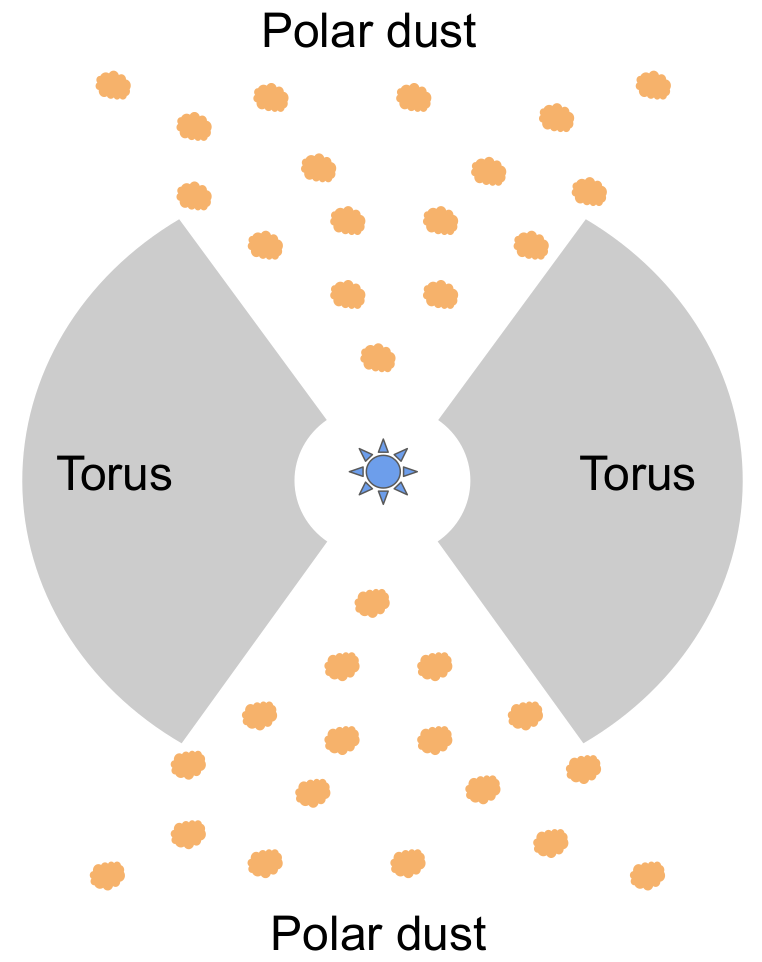
Figure 4: Schematic plot (at the meridional plane) of the AGN obscuration system adopted by X-CIGALE (not to scale). The model in original CIGALE only includes torus obscuration. We add the obscuration of polar dust to account for type 1 AGN extinction.

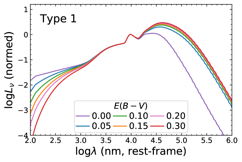
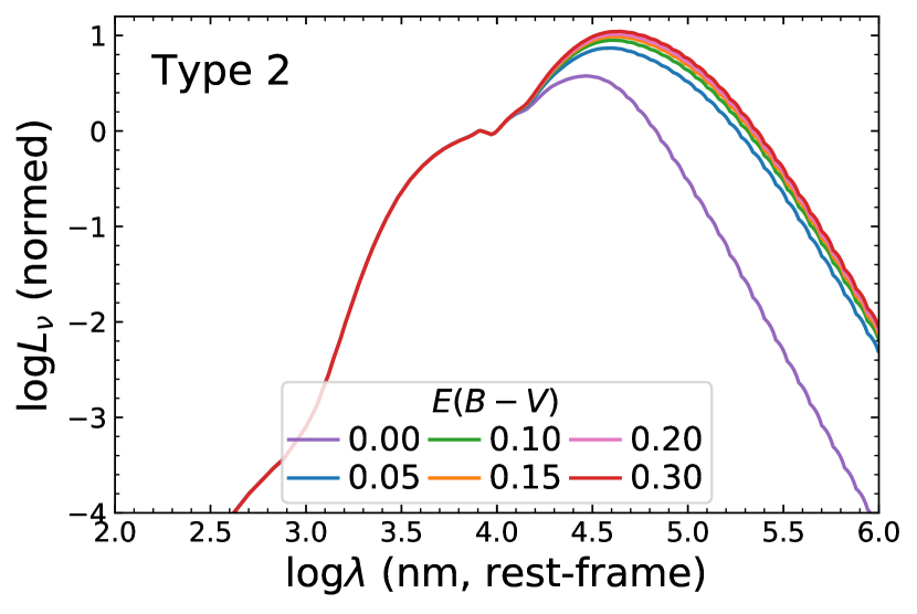
Figure 5: Same format as in Fig. 2, but for AGNs with different polar-dust $E(B-V)$. The top and bottom panels are for type 1 and type 2 AGNs, respectively. The SEDs are normalized at $10\ \mu$m. Except for $E(B-V)$, the other model parameters are the same (e.g. polar-dust temperature $=100$ K and emissivity $=1.6$) when generating these model SEDs.

3 Tests on X-ray detected sources

In this section, we test X-CIGALE with three samples of AGNs, i.e. SDSS (§3.1), COSMOS (§3.2), and AKARI-NEP (§LABEL:sec:akari). The basic properties of these samples are summarized in Table 1. These three samples have different characteristics. The SDSS sample is optically bright type 1 quasars. The COSMOS sample is X-ray selected AGNs with broad multiwavelength coverage from $u$ to Herschel/PACS 160 $\mu$m. This sample also has spectroscopic AGN classifications. The AKARI-NEP sample is small but has excellent MIR observations from AKARI.

Table 1: Sample properties

Name	$N$	$m_{r}$	$f_{\rm 2\text{--}10\ keV}$	Redshift	Type${}_{\rm AGN}$
SDSS	1986	19.2–20.9	2.2–10.5	0.6–1.9	1
COSMOS	590	21.3–23.7	0.4– 1.7	0.6–1.8	1 & 2
AKARI-NEP	74	20.5–23.4	0.6– 2.1	0.5–1.4	1 & 2

Note. — (1) Survey name. (2) Number of AGNs. (3) $r$-band AB magnitude range (20%–80% percentile). (4) 2–10 keV X-ray flux range (20%–80% percentile) in units of $10^{-14}$ erg s${}^{-1}$ cm${}^{-2}$. (5) Redshift range (20%–80% percentile). (6) Types of AGNs included in the survey.

3.1 SDSS

3.1.1 The sample and the models

The SDSS sample is optically selected from the DR14 quasar catalog (paris18). All the sources are spectroscopically confirmed type 1 AGNs. In addition to the SDSS $ugriz$ bands, the paris18 catalog provides X-ray data from XMM-Newton archival observations when available (the 3XMM catalog; rosen16). We require the sources to be detected in the 2–12 keV band at $>3\sigma$ significance levels. Here, the choice of the hard X-ray band (2–12 keV) is to minimize the effects of X-ray obscuration (see §2.2.1). We do not include the IR photometry compiled in the DR14 catalog, because our main goal here is to test X-CIGALE on the simple cases, i.e. the quasar-dominated SED. In the X-ray to optical wavelengths, the AGN component is dominant; but in the IR wavelengths, the galaxy component may be non-negligible. We discuss the cases of AGN-galaxy mixed SEDs in §3.2 and §LABEL:sec:akari. We require the sources to have Galactic extinctions estimated in the DR14 quasar catalog, because we need to correct for Galactic extinction before providing the photometry to X-CIGALE. These criteria lead to a final sample of 1986 AGNs (Table 1).

For the SDSS sample, we can neglect the galaxy SED component, because the sources are optically bright quasars which often dominate the observed UV/optical SEDs. The AGN-dominant (X-ray to IR) models in X-CIGALE can be achieved by setting ${\rm frac_{AGN}}$ to a value close to unity (e.g. 0.999). The adopted AGN model parameters are listed in Table 2. The only free parameter in our fitting is polar-dust $E(B-V)$, which affects the UV/optical SED shape. We further justify that it is necessary to have $E(B-V)$ as a free parameter in §3.1.2. Other SKIRTOR parameters are fixed, because they only affect the IR SED shape where there is no band coverage for the SDSS sample (see §LABEL:sec:res_akari for the assessment of these parameters).

For the X-ray module, we adopt $\Gamma=1.8$ for AGN (the dominant component in X-rays), the typical intrinsic photon index constrained by observations (§2.2.2). Adopting other AGN $\Gamma$ values (e.g. 1.4 or 2.0) do not affect our fitting results significantly. Our adopted $\Gamma=1.8$ is slightly different from that assumed in the 3XMM catalog ($\Gamma=1.7$; rosen16). Therefore, we scale the 2–12 keV fluxes by a factor of 0.96 to correct the effects of different $\Gamma$, and this correction factor is obtained using the PIMMS website. For the LMXB and HMXB components, we set $\Gamma=1.56$ and 2.0, respectively (see §2.2.2). We adopt $|\Delta\alpha_{\rm ox}|_{\rm max}=0.2$, and this $|\Delta\alpha_{\rm ox}|_{\rm max}$ value is $\approx 2\sigma$ scatter of the $\alpha_{\rm ox}$-$L_{2500\textup{\AA}}$ relation (§2.2.3). Note that although the X-ray module has both parameters fixed, X-CIGALE internally calculates 9 models of different $\alpha_{\rm ox}$ values and selects $|\Delta\alpha_{\rm ox}|\leq|\Delta\alpha_{\rm ox}|_{\rm max}$ (see §2.2.3).

Table 2: SDSS fitting parameters

Module	Parameter	Values
AGN (UV-to-IR): SKIRTOR	Torus optical depth at 9.7 microns $\tau_{9.7}$	7.0
	Torus density radial parameter $p$ ($\rho\propto r^{-p}\mathrm{e}^{-q|\cos(\theta)|}$)	1.0
	Torus density angular parameter $q$ ($\rho\propto r^{-p}\mathrm{e}^{-q|\cos(\theta)|}$)	1.0
	Angle between the equatorial plane and edge of the torus $\Delta$	40${}^{\circ}$
	Ratio of the maximum to minimum radii of the torus	20
	Viewing angle $\theta$ (face on: $\theta=0^{\circ}$, edge on: $\theta=90^{\circ}$)	30${}^{\circ}$
	AGN fraction in total IR luminosity ${\rm frac_{AGN}}$	0.999
	Extinction law of polar dust	SMC
	$E(B-V)$ of polar dust	0, 0.05, 0.1, 0.15, 0.2, 0.3
	Temperature of polar dust (K)	100
	Emissivity of polar dust	1.6
X-ray: This work	AGN photon index	1.8
	Maximum deviation from the $\alpha_{\rm ox}$-$L_{2500\textup{\AA}}$ relation $|\Delta\alpha_{\rm ox}|_{\rm max}$	0.2
	LMXB photon index	1.56
	HMXB photon index	2.0

3.1.2 Fitting results

We run X-CIGALE with the model settings in §3.1.1 for the SDSS sample. The median reduced $\chi^{2}$ ($\chi^{2}_{\rm red}$) and degrees of freedom (dof) are 1.4 and 5, respectively. These $\chi^{2}_{\rm red}$ and dof values correspond to a $p$-value of 23%, well above the conventional 2$\sigma$ (5%) or 3$\sigma$ (0.3%) values. This result indicates that X-CIGALE is able to model the observed photometry of the SDSS quasars. Fig. 6 shows a random example of the SED fitting. Fig. 7 displays the $E(B-V)$ distribution from the fitting. As expected (see §2.4.1), most (75%) SDSS AGNs have weak or no extinction with $E(B-V)\leq 0.1$.

To evaluate the effects of the new X-ray module, we re-run X-CIGALE but without this module. We compare the AGN intrinsic $L_{2500\textup{\AA}}$ between the fitting with X-ray ($L_{2500\textup{\AA},\rm X}$) vs. without X-ray ($L_{2500\textup{\AA},\rm noX}$) in Fig. 8. The $L_{2500\textup{\AA},\rm X}$ and $L_{2500\textup{\AA},\rm noX}$ are similar, and this similarity is as expected. SDSS sources are mostly unobscured type 1 AGNs due to their selection method (§2.4.1), and thus the intrinsic AGN emission is directly observable at UV/optical wavelengths. Therefore, adding the X-ray module does not significantly change $L_{2500\textup{\AA}}$ estimation for SDSS sources in general.

In Table 2, the only free parameter is polar-dust $E(B-V)$, because this parameter affects the UV/optical SED which is covered by the SDSS bands (§3.1.1). In other words, we consider that $E(B-V)$ can be constrained by the photometric data. The constrainability of a model parameter can be evaluated by the “mock analysis” of X-CIGALE, which already exists in the previous version of CIGALE (see §4.3 of boquien19 for details). Briefly, after fitting the observed data, X-CIGALE simulates a mock catalog based on the best-fit model for each object. The photometric uncertainties are considered when simulating the mock data. X-CIGALE then performs SED fitting to the mock catalog and obtains Bayesian-like estimated values (and their errors) of the parameter. By comparing these estimated values and those used to generate the mock catalog (i.e. the “true” values), one can assess whether the parameter can be reliably constrained. The mock analysis serves as a sanity check to assess whether a physical parameter can be retrieved in a self-consistent way. This mock analysis can be invoked by setting “mock_flag$=$True” in the X-CIGALE configurations.

We run the mock analysis to test if polar-dust $E(B-V)$ can be constrained. We compare the estimated and true values in Fig. 9 (left). The estimated and true values are well correlated, indicating that $E(B-V)$ can be self-consistently constrained. In Fig. 10, we show the PDF of $E(B-V)$ for the source in Fig. 6. Fig. 10 indicates that the $E(B-V)$ is indeed well constrained in the Bayesian-like analysis.

In our fitting, aside from the model normalization (automatically determined by X-CIGALE; see §4.3 of boquien19), $E(B-V)$ is the only free model parameter (Table 2). We also test freeing other parameters such as viewing angle and torus optical depth, and the mock-analysis results of $E(B-V)$ are similar. For example, Fig. 9 (right) shows the result after setting the viewing angle to 0–90${}^{\circ}$ with a step of 10${}^{\circ}$ (i.e. all allowed values). The estimated and true values are still well correlated, indicating that $E(B-V)$ and viewing angle are not strongly degenerate. This non-degeneracy is understandable, because, in our polar-dust model, $E(B-V)$ is the only parameter responsible for modelling the observed UV/optical SED shapes of type 1 AGNs like the SDSS objects (§2.4).

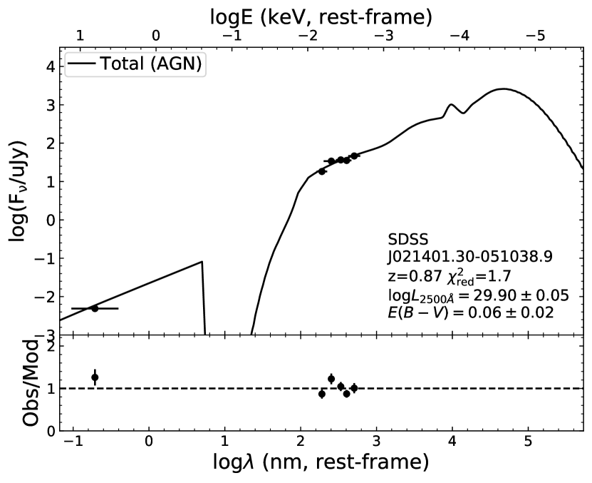
Figure 6: A random example of fitted SED from SDSS. The fitting residuals (observed flux/model flux) are shown at the bottom. Some source properties are labelled on the plot. Since the fitting only uses the AGN component, the total SED is actually the same as the AGN SED.

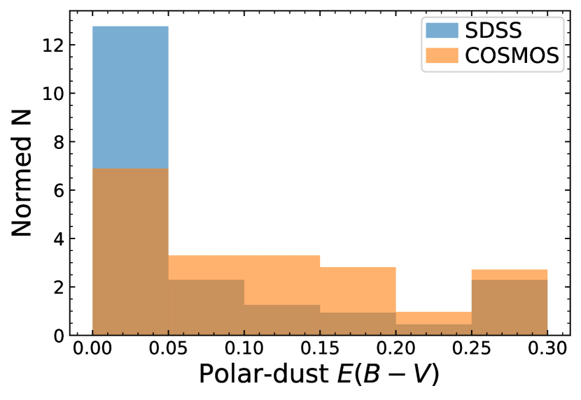
Figure 7: The distribution of AGN polar-dust $E(B-V)$ (Bayesian-like estimate) from X-CIGALE fitting for SDSS (blue) and COSMOS (orange) spectroscopic type 1 AGNs. The histogram is normalized such that the integral is unity. The COSMOS sources tend to have higher $E(B-V)$ than the SDSS sources.

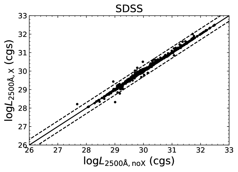
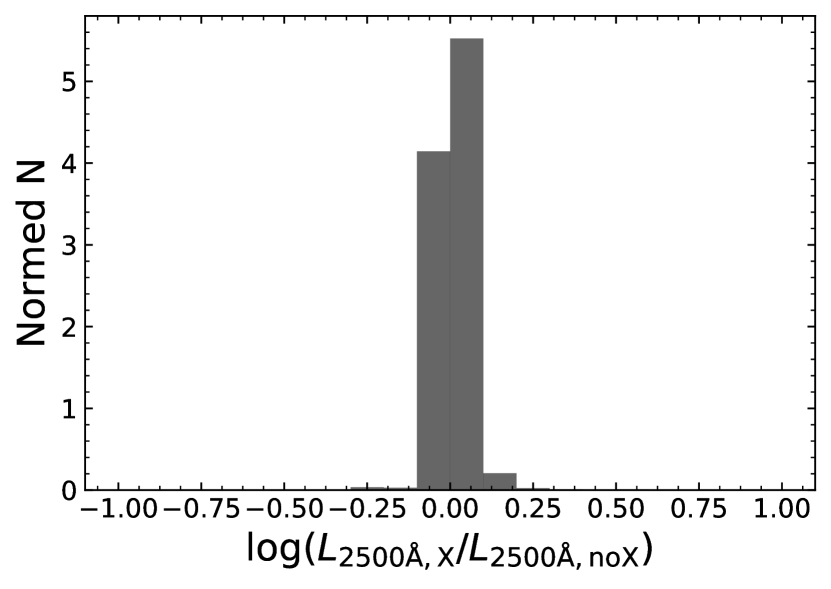
Figure 8: Top: Comparison of AGN intrinsic $L_{2500\textup{\AA}}$ between the fitting with X-ray vs. without X-ray for the SDSS sample. Here, the $L_{2500\textup{\AA}}$ values are Bayesian-like estimates of X-CIGALE fitting. The solid black lines indicate the 1:1 relation; the dashed black lines indicate 0.3 dex deviation from the 1:1 relation. Bottom: Distribution histogram of the $L_{2500\textup{\AA},\rm X}/L_{2500\textup{\AA},\rm noX}$ ratio for the SDSS sample. The histogram is normalized such that the integral is unity.

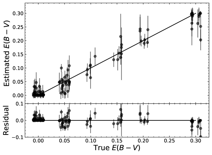
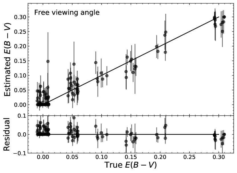
Figure 9: Left: Estimated vs. true values in the mock analyses of the SDSS sample for polar-dust $E(B-V)$. The black line indicates the 1:1 relation between estimated and true values. For clarity, the data points are from 100 randomly selected sources in the SDSS sample. The values on the $x$-axis are shifted slightly for display purposes only. The residuals (defined as estimated minus true) are displayed on the bottom panel, with the black line indicating a zero residual. For $E(B-V)$, the estimated and true values are well correlated, indicating that $E(B-V)$ model parameter can be effectively constrained by the data. Same format as left but from the fitting with free viewing angle.

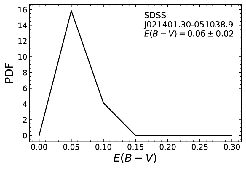
Figure 10: The $E(B-V)$ PDF for the example source in Fig. 6. The PDF is normalized such that its integral is unity.

3.2 COSMOS

3.2.1 The sample and the models

The COSMOS sample is X-ray selected ($>3\sigma$, 2–10 keV band) from the COSMOS-Legacy survey performed by Chandra (civano16). The COSMOS-Legacy catalog assumes $\Gamma=1.4$. Similarly as in §3.1.1, we apply a correction factor of 0.87 (calculated with PIMMS) to the 2–10 keV fluxes to make them consistent with our adopted $\Gamma=1.8$ for AGN. marchesi16 matched these X-ray sources with the optical/NIR counterparts in the COSMOS2015 catalog (laigle16) and compiled their spectroscopic information when available. We select the sources with spectroscopic classifications of AGN types. We adopt the photometric data in the COSMOS2015 catalog, including 14 broad bands from $u$ to IRAC 8.0 $\mu$m. In addition, when available, we also include photometric data from Spitzer/MIPS (24 $\mu$m) and Herschel/PACS (100 $\mu$m and 160 $\mu$m), from the PEP survey (lutz11). We adopt the redshift measurements from marchesi16. These redshifts are either secure spectroscopic redshifts or high-quality photometric redshifts. There are a total of 590 objects in COSMOS (Table 1). Among these 590 objects, 206 and 384 are type 1 and type 2 AGNs, respectively.

The X-CIGALE model parameters for COSMOS are listed in Table 3. For the SKIRTOR and X-ray modules, the parameter setting is the same as in §3.1.1 except for ${\rm frac_{AGN}}$ and the viewing angle. Here, we allow ${\rm frac_{AGN}}$ to vary among 0.01, 0.1–0.9 (step 0.1), and 0.99, because, unlike in the case of SDSS, the AGN contribution to the observed SED may not be generally not dominant for the COSMOS sample, especially in the IR bands. We set the viewing angle to 30${}^{\circ}$ and 70${}^{\circ}$ for the spectroscopic type 1 and type 2 AGNs, respectively. These values are approximately the probability-weighted $\theta$ for type 1 and type 2 AGNs, respectively, given a torus of $\Delta=40^{\circ}$ (see 2.2.3).

For the galaxy component, we adopt the model setting similar to that in ciesla15. Specifically, we adopt a delayed star-formation history (SFH), because it can characterize the SEDs of both early-type and late-type galaxies reliably (e.g. ciesla15; boquien19). Also, the delayed SFH only has relatively small parameter space (only two free parameters) and thereby high fitting efficiency. We adopt a chabrier03 IMF with metallicity ($Z$) fixed to the solar value of 0.02. For the galactic dust attenuation, we adopt the dustatt_calzleit module in X-CIGALE (calzetti00; leitherer02). The allowed $E(B-V)$ values for young stars are 0.1, 0.2, 0.3, 0.4, 0.5, 0.7, and 0.9. The $E(B-V)$ ratio between the old and young stars is fixed to 0.44. The amplitude of the 217.5 nm UV bump on the extinction curve is set to 0 (SMC) and 3 (Milky Way). We adopt the dale14 model for galactic dust reemission. There is only one free parameter in this model, i.e. the $\alpha$ slope in $dM_{\rm dust}\propto U^{-\alpha}dU$, where $M_{\rm dust}$ and $U$ are dust mass and radiation-field intensity, respectively. The $\alpha$ values are set to 1.5, 2.0, and 2.5.

Table 3: COSMOS and AKARI-NEP Fitting Parameters

Module	Parameter	Values
Star formation history: delayed model, $\mathrm{SFR}\propto t\exp(-t/\tau)$	$e$-folding time, $\tau$ (Gyr)	0.1, 0.5, 1, 5
	Stellar Age, $t$ (Gyr)	0.5, 1, 3, 5, 7
Simple stellar population: bruzual03	Initial mass function	chabrier03
	Metallicity ($Z$)	0.02
Galactic dust attenuation: calzetti00 & leitherer02	$E(B-V)$ of starlight for the young population	0.1, 0.2, 0.3, 0.4, 0.5, 0.7, 0.9
	$E(B-V)$ ratio between the old and young populations	0.44
Galactic dust emission: dale14	$\alpha$ slope in $dM_{\rm dust}\propto U^{-\alpha}dU$	1.5, 2.0, 2.5
AGN (UV-to-IR): SKIRTOR	Torus optical depth at 9.7 microns $\tau_{9.7}$	7.0
	Torus density radial parameter $p$ ($\rho\propto r^{-p}\mathrm{e}^{-q|\cos(\theta)|}$)	1.0
	Torus density angular parameter $q$ ($\rho\propto r^{-p}\mathrm{e}^{-q|\cos(\theta)|}$)	1.0
	Angle between the equatorial plan and edge of the torus	40${}^{\circ}$
	Ratio of the maximum to minimum radii of the torus	20
	Viewing angle $\theta$ (face on: $\theta=0^{\circ}$, edge on: $\theta=90^{\circ}$)${}^{a}$	30${}^{\circ}$ (type 1), 70${}^{\circ}$ (type 2)
	AGN fraction in total IR luminosity ${\rm frac_{AGN}}$	0.01, 0.1–0.9 (step 0.1), 0.99
	Extinction law of polar dust	SMC
	$E(B-V)$ of polar dust	0, 0.05, 0.1, 0.15, 0.2, 0.3
	Temperature of polar dust (K)	100
	Emissivity of polar dust	1.6
X-ray: This work	AGN photon index $\Gamma$	1.8
	Maximum deviation from the $\alpha_{\rm ox}$-$L_{2500\textup{\AA}}$ relation	0.2
	LMXB photon index	1.56
	HMXB photon index	2.0

Note. — ($a$) For COSMOS, the viewing angles are set to 30${}^{\circ}$ and 70${}^{\circ}$ for the spectroscopic type 1 and type 2 AGNs, respectively. For AKARI-NEP, we allow X-CIGALE to choose between 30${}^{\circ}$ and 70${}^{\circ}$ for the entire sample, since spectroscopic classifications are not available.