Computation of effective front form Hamiltonians for massive Abelian gauge theory

Abstract

Renormalization group procedure for effective particles (RGPEP) is applied in terms of a second-order perturbative computation to an Abelian gauge theory, as an example of application worth studying on the way toward derivation of a dynamical connection between the spectroscopy of bound states and their parton-model picture in the front form of Hamiltonian dynamics. In addition to the ultraviolet transverse divergences that are handled using the RGPEP in previously known ways, the small-x divergences are handled by introducing a mass parameter and a third polarization state for gauge bosons using a mechanism analogous to spontaneous breaking of global gauge symmetry, in a special limit that simplifies the theory to Soper’s front form of massive QED. The resulting orders of magnitude of scales involved in the dynamics of effective constituents or partons in the simplified theory are identified for the fermion and boson mass counter terms, effective masses and self-interactions, as well as for the Coulomb-like effective interactions in bound states of fermions. Computations in orders higher than second are mentioned but not described in this article.

I Introduction

Particle theory singularities that are associated with wee partons of the parton model of hadrons FeynmanPM or with field quanta that carry small kinematic momenta in the front form (FF) of Hamiltonian dynamics DiracFF , require a renormalization group procedure that is capable of simultaneous handling of the ultraviolet and infrared divergences in combination with the bound-state problem, which is a complex issue Wilsonetal . One way of approaching the issue has been proposed recently AbelianAPPB in the context of Abelian gauge theory. The idea is to use a mechanism analogous to spontaneous breaking of global gauge symmetry Higgs1 ; EnglertBrout for introducing a mass for gauge bosons and to thus regulate the theory in the region in question. This article pursues that idea in terms of a study of the kind and magnitude of Hamiltonian interaction terms it leads to in the effective theories. Our work is carried out in a special limit that simplifies the Abelian theory to Soper’s FF version of massive QED Soper . The theory does not include confinement but it does provide examples of effective interactions that bind fermions.

It should be noted that gauge theories with Lagrangian densities similar to Soper’s were introduced for analysis in the instant form (IF)[2] of dynamics a long time ago Stueckelberg ; Matthews ; Coester ; Salam ; Kamefuchi . In the FF of dynamics, Soper’s work was followed by Yan’s Yan3 ; Yan4 . For a review of more recent works that use massive vector bosons as ultraviolet or infrared regulators in FF approaches, see Hiller and references therein. Soper found that the replacement of photons in FF of QED by massive vector bosons is quite simple if one considers in addition to the vector field $A^{\mu}$ in gauge $A^{+}=0$ a scalar field $B$ in the manner of Stueckelberg Stueckelberg . The Stueckelberg formalism was also used in FF calculations of transition matrix elements in the Feynman gauge LFStueckelberg . Perhaps similar attempts could be undertaken also in the non-Abelian theories KunimasaGoto . In view of that extensive record, it should be stated up front in what way the present study differs from the previous ones. We start from a different Lagrangian than massive QED and in the manner analogous to spontaneous breaking of global gauge invariance arrive at Soper’s theory as a helpful simplification in a special limit. Subsequently, instead of aiming at reproducing or predicting observables directly in terms of the degrees of freedom that appear in canonical FF Hamiltonian in a diverging way, our goal is to compute the equivalent effective FF Hamiltonian operators that are written in terms of apparently more adequate degrees of freedom [18,19]. Computation of such Hamiltonians is hoped to eventually lead to a sequence of successive approximations for relativistic description of strongly bound states because they do not diverge as the canonical FF Hamiltonians do, see Sec. IV for details. Soper’s theory serves as a preliminary illustration of the magnitude of terms one has to deal with. Little is known at this point regarding extension of our approach to non-Abelian theories. However, since the mechanism of spontaneous breaking of global gauge symmetry serves the purpose of regularization and when one lifts the regularization the symmetry may be restored, the author hopes that the current exercise with Soper’s theory will turn out helpful also in studying non-Abelian theories.

To compute effective FF Hamiltonians for the massive Abelian gauge theory, we use the renormalization group procedure for effective particles (RGPEP), here only applied up to the second order in a series expansion in powers of the coupling constant RGPEP . The RGPEP stems from the similarity renormalization group (SRG) procedure GlazekWilson and draws on the double-commutator differential flow equation for Hamiltonian matrices Wegner . The method preserves boost-invariance of the FF of Hamiltonian dynamics and its computations are carried out in terms of the quantum fields on one light-front hyperplane in space-time. We calculate the mass counter terms, effective fermion and boson mass corrections, relativistic fermion-anti-fermion interaction terms that correspond to the well-known Yukawa or Coulomb potentials and additional terms that do not have classical counterparts.

Section II introduces the classical gauge theory we consider. The canonical FF version of the theory and its quantization are described in Sec. III. The RGPEP is applied in Sec. IV, where we compute the effective fermion and boson self-interactions and relativistic potentials in fermion-anti-fermion systems. Section V discusses the connection between spectroscopy and the parton-model picture of bound states in the context of the RGPEP. Detailed plots of mass corrections and relativistic potentials are given in Sec. VI. The paper is concluded by Sec. VII. Appendixes provide details of our notation and the canonical Hamiltonian of Soper’s theory.

II Classical theory

The FF Hamiltonian for the theory we consider was recently derived AbelianAPPB from the familiar local Lagrangian density Higgs1 ; EnglertBrout ; Kibble

$${\cal L} = {\cal L}_{\psi}+{\cal L}_{A}+{\cal L}_{A\phi}-{\cal V}_{\phi}\ ,$$ (1)

where

$${\cal L}_{\psi} = \bar{\psi}\left[\left(i\partial_{\mu}-gA_{\mu}\right)\gamma^{\mu}-m\right]\psi\ ,$$ (2)

$${\cal L}_{A} = -{1\over 4}F_{\mu\nu}F^{\mu\nu}\ ,$$ (3)

$${\cal L}_{A\phi} = \left[(i\partial^{\mu}-g^{\prime}A^{\mu})\phi\right]^{\dagger}(i\partial_{\mu}-g^{\prime}A_{\mu})\phi\ ,$$ (4)

$${\cal V}_{\phi} = -\mu^{2}\ \phi^{\dagger}\phi+{\lambda^{2}\over 2}\ (\phi^{\dagger}\phi)^{2}\ .$$ (5)

Quanta of field $\psi$ will correspond to fermions and quanta of field $A$ to transversely polarized gauge bosons. Quanta of the phase of scalar field $\phi$ will supply effects associated with the longitudinal polarization of massive gauge bosons. This section briefly recapitulates derivation of the corresponding FF Hamiltonian and presents it in a special limit in which it matches the Hamiltonian designed by Soper for the FF of massive QED, a long time ago Soper . Further literature on the use of FF quantum dynamics can be traced through reviews Hiller ; FFreview1 ; FFreview2 ; FFreview3 ; FFreview4 ; FFreview5 ; FFreview6 .

II.1 Gauge symmetry

Field $\phi$ in the Lagrangian density of Eq. (4) can be written using its modulus $|\phi|=\varphi/\sqrt{2}$ and phase $g^{\prime}\theta$ Kibble ,

$$\phi = \varphi\ e^{ig^{\prime}\theta}/\sqrt{2}\ .$$ (6)

The density ${\cal L}_{A\phi}$ is a function of $\varphi$, $\partial^{\mu}\varphi$ and $\partial^{\mu}\theta$

$${\cal L}_{A\phi} = \,{1\over 2}\,(\partial^{\mu}\varphi)^{2}+\,{1\over 2}\,g^{\prime 2}(A^{\mu}+\partial^{\mu}\theta)^{2}\varphi^{2}\ .$$ (7)

The modulus field can be written as $\varphi=v+h$, where $v$ will be treated as a parameter of the FF theory and the field $h$ may vary in space-time. When one sets $h=0$, the potential ${\cal V}_{\phi}$ in Eq. (5) has its minimal value $-\mu^{4}/(2\lambda^{2})$ for $v=\sqrt{2}\ \mu/\lambda$. Using this special value of $v$, one has

$${\cal V}(\phi)\,=\,-{\mu^{4}\over 2\lambda^{2}}+\,{1\over 2}\,\,(\sqrt{2}\,\mu)^{2}\ h^{2}+{\lambda\over\sqrt{2}}\ \mu\ h^{3}+{\lambda^{2}\over 8}\ h^{4}\ .$$ (8)

The Lagrangian density of Eq. (1) is invariant under substitutions

$$\psi = e^{-igf}\tilde{\psi}\ ,$$ (9)

$$A^{\mu} = \tilde{A}^{\mu}+\partial^{\mu}f\ ,$$ (10)

$$\varphi = \tilde{\varphi}\ ,$$ (11)

$$\theta = \tilde{\theta}-f\ .$$ (12)

The meaning of this invariance is that the Lagrangian density is the same function of fields with and without the tilde. The corresponding minimal coupling that appears in a quantum theory obtained using the RGPEP, will be discussed in Sec. IV.2, see Eqs. (60) and (61).

II.2 Massive limit

Consider the limit of $g^{\prime}\to 0$, $v\to\infty$ and $g^{\prime}v=\kappa$ kept constant, which will be called the massive limit. In this limit,

$${\cal L}_{A\phi} = \,{1\over 2}\,(\partial^{\mu}h)^{2}+\,{1\over 2}\,\kappa^{2}(A^{\mu}+\partial^{\mu}\theta)^{2}\ ,$$ (13)

$${\cal V}_{\phi} = -{\mu^{4}\over 2\lambda^{2}}+\,{1\over 2}\,\,(\sqrt{2}\,\mu)^{2}\ h^{2}\ .$$ (14)

The field $h$ decouples and retains an arbitrary mass $\sqrt{2}\ \mu$.

II.3 Gauge choice $f=-\theta$

Using $f=-\theta$ one obtains

$${\cal L}_{\psi} = \bar{\tilde{\psi}}\left[\left(i\partial_{\mu}-g\tilde{A}_{\mu}\right)\gamma^{\mu}-m\right]\tilde{\psi}\ ,$$ (15)

$${\cal L}_{A} = -{1\over 4}\tilde{F}_{\mu\nu}\tilde{F}^{\mu\nu}\ ,$$ (16)

$${\cal L}_{A\phi} = \,{1\over 2}\,(\partial^{\mu}\tilde{\varphi})^{2}+\,{1\over 2}\,g^{\prime 2}\tilde{A}^{\mu\,2}\tilde{\varphi}^{2}\ ,$$ (17)

$${\cal V}_{\phi} = {\cal V}(\tilde{\varphi}/\sqrt{2})\ .$$ (18)

In the massive limit, ${\cal L}_{A\phi}$ is

$${\cal L}_{A\phi} = \,{1\over 2}\,(\partial^{\mu}\tilde{h})^{2}+\,{1\over 2}\,\kappa^{2}\tilde{A}^{2}\ ,$$ (19)

the potential ${\cal V}_{\phi}$ reduces to $\mu^{2}\tilde{h}^{2}$ plus a constant $\mu^{2}/(2\lambda^{2})$ that can be ignored, while the densities ${\cal L}_{\psi}$ and ${\cal L}_{A}$ remain unchanged. The resulting action corresponds to a free scalar field $\tilde{h}$ of mass $\sqrt{2}\,\mu$ and a vector field $\tilde{A}$ of mass $\kappa$ minimally coupled to the fermion field $\tilde{\psi}$. The massive-limit theory with field $\tilde{h}$ removed turns out to be the same as Soper’s Soper when one identifies his field $B$ with our $-\kappa\theta$ and his mass parameter $\kappa$ with our $\kappa=g^{\prime}v$.

If the gauge symmetry under consideration were realized in nature and photons indeed had a very small mass $\kappa$, which is theoretically possible GoldhaberNieto , there would also exist a decoupled scalar field $h$ of unknown mass, as the FF of the theory in the massive limit indicates, too. According to PDG , the photon mass is smaller than $10^{-18}$eV/$c^{2}$. Searches for new forms of matter are motivated by data concerning the structure and evolution of the universe, besides questions concerning the standard model.

III Canonical FF Hamiltonian

In the FF of dynamics, the space-time coordinate $x^{+}=x^{0}+x^{3}$ is used as the evolution parameter analogous to time in the instant form (IF) DiracFF . The coordinates $x^{-}=x^{0}-x^{3}$ and $x^{\perp}=(x^{1},x^{2})$ parameterize points on the space-time hyperplanes that are defined by fixed values of $x^{+}$. These hyperplanes are called “light fronts” or just “fronts,” such as the front defined by the condition $x^{+}=0$. Evolution in $x^{+}$ from the front at $x^{+}=0$ to other fronts is generated by the Hamiltonian $P^{-}$.

Field theory relates the Lagrangian density of Eq. (1) to the corresponding Hamiltonian density through the energy-momentum tensor density $T^{\mu\nu}$,

$$T^{\mu\nu} = \sum_{\chi}{\partial{\cal L}\over\partial\partial_{\mu}\chi}\ \partial^{\nu}\chi-g^{\mu\nu}{\cal L}\ ,$$ (20)

where $\chi$ stands for a field in a theory. The FF Hamiltonian density is ${\cal H}=T^{+\,-}/2$ and the Hamiltonian $P^{-}$ is given by KogutSoper ; Yan3

$$P^{-} = \int d^{2}x^{\perp}dx^{-}\ {\cal H}\ .$$ (21)

where the integral extends over the front at $x^{+}=0$. The Lagrangian density of Eq. (1) is linear in $\partial^{-}f$ and the Hamiltonian density is ${\cal H}=-{\cal L}(\partial^{-}f\to 0)$. For constructing a quantum theory, one needs to evaluate ${\cal H}$ in terms of the fields’ independent degrees of freedom.

III.1 Equations of motion and gauge $\tilde{A}^{+}=0$

The principle of minimal action with the Lagrangian desity of Eq. (1) implies the Euler-Lagrange (EL) equations that, when written in terms of the fields $\psi$, $A$, $\varphi$ and $B=-\kappa\theta$, read

$$\left[\left(i\partial_{\mu}-gA_{\mu}\right)\gamma^{\mu}-m\right]\psi = 0\ ,$$ (22)

$$\Box A^{\beta}-\partial^{\beta}\,\partial_{\alpha}A^{\alpha} = g\bar{\psi}\gamma^{\beta}\psi-g^{\prime 2}\ \varphi^{2}\ (A^{\beta}-\kappa^{-1}\partial^{\beta}B)\ ,$$ (23)

$$\Box\varphi = g^{\prime 2}\ \varphi\ (A^{\beta}-\kappa^{-1}\partial^{\beta}B)^{2}-{\partial{\cal V}(\varphi/\sqrt{2})\over\partial\varphi}\ ,$$ (24)

$$\partial_{\mu}g^{\prime 2}\varphi^{2}(A^{\mu}-\kappa^{-1}\partial^{\mu}B) = 0\ .$$ (25)

The last equation is necessarily satisfied if the first two are. The first equation can be written in terms of the fermion field arranged according to the formula $\psi=\psi_{+}+\psi_{-}$, where $\psi_{\pm}=\Lambda_{\pm}\psi$ and $\Lambda_{\pm}=\,{1\over 2}\,\gamma^{0}\gamma^{\pm}=\,{1\over 2}\,(1\pm\alpha^{3})$ are $4\times 4$ projection matrices. In these terms, the fermion EL equation is equivalent to two coupled equations,

$$(i\partial^{-}-gA^{-})\psi_{+}-\left[(i\partial^{\perp}-gA^{\perp})\alpha^{\perp}+m\beta\right]\psi_{-} = 0\ ,$$ (26)

$$(i\partial^{+}-gA^{+})\psi_{-}-\left[(i\partial^{\perp}-gA^{\perp})\alpha^{\perp}+m\beta\right]\psi_{+} = 0\ .$$ (27)

Using gauge symmetry, one can transform the fields $\psi$, $A$, $\varphi$ and $B$ to $\tilde{\psi}$, $\tilde{A}$, $\tilde{\varphi}$ and $\tilde{B}$. The two coupled fermion equations have the same form in terms of the fields with tilde and without tilde. However, if the gauge transformation sets the field $\tilde{A}^{+}$ to zero, then

$$\tilde{\psi}_{-} = {1\over i\partial^{+}}\left[(i\partial^{\perp}-g\tilde{A}^{\perp})\alpha^{\perp}+m\beta\right]\tilde{\psi}_{+}\ .$$ (28)

The field $\tilde{\psi}_{-}$ on a front is thus given in terms of the fields $\tilde{\psi}_{+}$ and $\tilde{A}^{\perp}$ on the same front. Similarly, the EL Eq. (23) for $\beta=+$ in the gauge $\tilde{A}^{+}=0$ constrains the field $\tilde{A}^{-}$,

$$\tilde{A}^{-} = {2\over\partial^{+}}\partial^{\perp}\tilde{A}^{\perp}-{2\over\partial^{+\,2}}\left(g\bar{\tilde{\psi}}\gamma^{+}\tilde{\psi}+g^{\prime 2}\ \tilde{\varphi}^{2}\ \kappa^{-1}\partial^{+}\tilde{B}\right)\ .$$ (29)

As a consequence of the constraints, the FF Hamiltonian density is a function of fields $\tilde{\psi}_{+}$, $\tilde{A}^{\perp}$, $\tilde{B}$ and $\tilde{\varphi}$.

III.2 Hamiltonian density ${\cal H}$

We use the Lagrangian density ${\cal L}$ of Eq. (1) written in terms of the independent field degrees of freedom $\tilde{\psi}_{+}$, $\tilde{A}^{\perp}$, $\tilde{B}$ and $\tilde{\varphi}$, to evaluate the Hamiltonian density using Eq. (20) for $T^{+-}=2{\cal H}$. From now on, we omit the tilde and employ notation $\varphi=v+h$ and $\kappa=g^{\prime}v$. We also introduce the fields $\psi_{f}$ and $A_{f}$ that are given by the constraint Eqs. (28) and (29) in the absence of interaction LepageBrodsky ,

$$A_{f}^{-} = {2\over\partial^{+}}\partial^{\perp}A^{\perp}\ ,\quad A_{f}^{+}\,=\,0\ ,\quad A_{f}^{\perp}\,=\,A^{\perp}\ ,$$ (30)

$$\psi_{f+} = \psi_{+}\ ,\quad\psi_{f-}\,=\,{1\over i\partial^{+}}\ \left[\alpha^{\perp}\,i\partial^{\perp}+m\beta\right]\psi_{+}\ .$$ (31)

The Hamiltonian density reads

$${\cal H} = \,{1\over 2}\,\left\{{1\over\partial^{+}}\left[g\bar{\psi}\gamma^{+}\psi-2\kappa B\,(1+h/v)\,\partial^{+}h/v\right]\right\}^{2}$$ (32)

$$+ (1+h/v)^{2}\kappa B\ {1\over\partial^{+}}\left[g\bar{\psi}\gamma^{+}\psi-2\kappa B\,(1+h/v)\,\partial^{+}h/v\right]$$

$$+ \bar{\psi}_{f}\,{1\over 2}\,\gamma^{+}{(i\partial^{\perp})^{2}+m^{2}\over i\partial^{+}}\psi_{f}+g\bar{\psi}_{f}\not A_{f}\psi_{f}+\,{1\over 2}\,g^{2}\bar{\psi}_{f}\not A_{f}{\gamma^{+}\over i\partial^{+}}\not A_{f}\psi_{f}$$

$$- \,{1\over 2}\,A_{f}^{\mu}\left[(i\partial^{\perp})^{2}+\kappa^{2}(1+h/v)^{2}\right]A_{f\mu}+(1+h/v)^{2}\kappa\ A_{f}^{\mu}\ \partial_{\mu}B$$

$$+ \,{1\over 2}\,h\left[(i\partial^{\perp})^{2}+(\sqrt{2}\,\mu)^{2}\right]h+{\mu^{2}\over v}h^{3}+\left({\mu\over 2v}\right)^{2}h^{4}-(\mu v/2)^{2}$$

$$+ \,{1\over 2}\,(1+h/v)^{2}\ B\left[(i\partial^{\perp})^{2}+\kappa^{2}(1+h/v)^{2}\right]B-(1+h/v)B\ \partial^{\perp}B\ \partial^{\perp}h/v\ .$$

It differs from Soper’s, because it involves additional fields. However, in the massive limit that ignores quantum effects, see Sec. II.2, in which $g^{\prime}\to 0$, $v\to\infty$, $g^{\prime}v=\kappa$ is kept constant (we could also consider the additional limit $\mu v\to 0$ to eliminate the constant $-(\mu v/2)^{2}$ and hence arrive at massless $h$), one obtains

$${\cal H} \to \,{1\over 2}\,\left[{1\over\partial^{+}}g\bar{\psi}\gamma^{+}\psi\right]^{2}+\kappa B\ {1\over\partial^{+}}\ g\bar{\psi}\gamma^{+}\psi$$ (33)

$$+ \bar{\psi}_{f}\,{1\over 2}\,\gamma^{+}{(i\partial^{\perp})^{2}+m^{2}\over i\partial^{+}}\psi_{f}+g\bar{\psi}_{f}\not A_{f}\psi_{f}+\,{1\over 2}\,g^{2}\bar{\psi}_{f}\not A_{f}{\gamma^{+}\over i\partial^{+}}\not A_{f}\psi_{f}$$

$$+ \,{1\over 2}\,A_{f}^{i}\left[(i\partial^{\perp})^{2}+\kappa^{2}\right]A_{f}^{i}+\kappa\ A_{f}^{\mu}\ \partial_{\mu}B$$

$$+ \,{1\over 2}\,h\left[(i\partial^{\perp})^{2}+(\sqrt{2}\,\mu)^{2}\right]h$$

$$+ \,{1\over 2}\,\ B\left[(i\partial^{\perp})^{2}+\kappa^{2}\right]B\ .$$

The second term, with the field $B$ and fermion plus current, can be replaced by the one that is equivalent through integration by parts. Since $A_{f}^{+}=0$ and $\partial_{\mu}A_{f}^{\mu}=0$, the seventh term that couples field $A_{f}$ to the gradient of filed $B$ is equivalent to zero. The decoupled field $h$ will be ignored in further discussion. Thus, one obtains the Hamiltonian density that is precisely equivalent to Soper’s for massive QED Soper . It can be written as

$${\cal H} = \bar{\psi}_{f}\gamma^{+}{(i\partial^{\perp})^{2}+m^{2}\over 2i\partial^{+}}\psi_{f}+\,{1\over 2}\,A_{f}^{i}\left[(i\partial^{\perp})^{2}+\kappa^{2}\right]A_{f}^{i}+\,{1\over 2}\,\ B\left[(i\partial^{\perp})^{2}+\kappa^{2}\right]B$$ (34)

$$+ g\bar{\psi}_{f}\not A_{f}\psi_{f}-g\bar{\psi}_{f}\gamma^{+}\psi_{f}{\kappa\over i\partial^{+}}iB+\,{1\over 2}\,g^{2}\bar{\psi}_{f}\not A_{f}{\gamma^{+}\over i\partial^{+}}\not A_{f}\psi_{f}+\,{1\over 2}\,\left[{1\over\partial^{+}}g\bar{\psi}_{f}\gamma^{+}\psi_{f}\right]^{2}\ .$$

If the coupling constant $g$ were set to zero, the first three terms would describe the free fermion field $\psi_{f}$, free gauge boson field $A_{f}$ with two polarizations and a free scalar field $B$. The fourth and fifth terms describe the minimal coupling of fields $A_{f}$ and $B$ with fermions, respectively. The sixth term additionally couples transverse bosons to fermions as a result of the constraint Eq. (28). The last term is the FF fermion quartic interaction that results from the constraint Eq. (29). It is a FF analog of the Coulomb term in the IF dynamics with its Gauss law. The Hamiltonian density of Eq. (34) is taken as a starting point for the canonical construction of a quantum theory a la Refs. Soper ; KogutSoper ; Yan3 .

III.3 Quantization

The quantum theory is introduced by replacing the fields $\psi_{f}$, $A_{f}$ and $B$ in Eq. (34) by the corresponding field operators on the front at $x^{+}=0$,

$$\hat{\psi}_{f} = \sum_{\sigma=1}^{2}\int[p]\left[u_{p\sigma}\hat{b}_{p\sigma}e^{-ipx}+v_{p\sigma}\hat{d}^{\dagger}_{p\sigma}e^{ipx}\right]_{x^{+}=0}\ ,$$ (35)

$$\hat{A}_{f}^{\mu} = \sum_{\sigma=1}^{2}\int[p]\left[\varepsilon^{\mu}_{p\sigma}\hat{a}_{p\sigma}e^{-ipx}+\varepsilon^{\mu*}_{p\sigma}\hat{a}^{\dagger}_{p\sigma}e^{ipx}\right]_{x^{+}=0}\ ,$$ (36)

$$\hat{B} = \int[p]\left[-i\hat{a}_{p3}e^{-ipx}+i\hat{a}^{\dagger}_{p3}e^{ipx}\right]_{x^{+}=0}\ ,$$ (37)

where $[p]=dp^{+}\theta(p^{+})d^{2}p^{\perp}/[2p^{+}(2\pi)^{3}]$. Further, $u_{p\sigma}$ and $v_{p\sigma}$ are spinors for fermions of mass $m$ LepageBrodsky ; fermions . Symbols $\varepsilon_{p\sigma}$ denote polarization four-vectors for bosons Soper ; AbelianAPPB . Thus, $\sigma$ labels fermions and gauge bosons that at rest have spin projections $\pm\,{1\over 2}\,$ or $\pm 1$ on the $z$-axis, respectively. Further details of the notation are explained in App. A. The creation and annihilation operators, denoted by $b$, $d$ and $a$, obey commutation or, in the case of fermions, anti-commutation relations of the form

$$[\hat{a}_{p\lambda},\hat{a}^{\dagger}_{q\sigma}] = 2p^{+}(2\pi)^{3}\delta(p^{+}-q^{+})\delta^{2}(p^{\perp}-q^{\perp})\delta_{\lambda\sigma}\ ,$$ (38)

with other commutators or anti-commutators equal zero. The Hamiltonian $\hat{P}^{-}$ is obtained by integrating the quantum density $\hat{\cal H}$ on the front $x^{+}=0$ and normal ordering.

At this point it is important to mention, on the basis of hindsight, that the operators creating or annihilating quanta with infinitesimal $p^{+}$, i.e., $p^{+}$ negligible in comparison with mass parameters $m$ and $\kappa$, including the case of $\kappa/m\to 0$, could contribute divergences to the free invariant masses of all physical states. Therefore, in the regulated and subsequently renormalized theory such quanta need to be suppressed. Formally, at this point one could introduce in Eqs. (35), (36) and (37) an infinitesimal cutoff parameter $\epsilon^{+}$, imposing a condition $p^{+}>\epsilon^{+}$ instead of $p^{+}>0$. However, it will become self-evident in the next sections that, in the RGPEP, perturbatively calculated effective Hamiltonians for finite-size quanta with finite plus momenta are not sensitive at all to the cutoff parameter $\epsilon^{+}\to 0$. Namely, it is shown in the next sections that the gauge boson mass $\kappa$ provides the required suppression through the vertex form factors that result from solving the RGPEP evolution Eq. (41). Regarding the divergent constants and one-particle operators that result from the normal ordering, they are dropped because constants do not count in the quantum dynamics and one-particle operators require counter terms anyway. In summary, the cutoff on $p^{+}$ and normal ordering do not influence the content of a theory defined using the RGPEP.

III.4 Quantum Hamiltonian

Our initial quantum Hamiltonian $\hat{P}^{-}$ is denoted by $\hat{H}$,

$$\hat{H} = \hat{H}_{\psi^{2}}+\hat{H}_{A^{2}}+\hat{H}_{B^{2}}+\hat{H}_{\psi A\psi}+\hat{H}_{\psi B\psi}+\hat{H}_{\psi AA\psi}+\hat{H}_{(\psi\psi)^{2}}\ .$$ (39)

The seven operators appear in one-to-one correspondence to the seven terms in Eq. (34). To simplify notation for the quantum theory, the operator symbol  $\hat{}$  is omitted in further formulas. The first three terms are separately denoted by

$$H_{f} = H_{\psi^{2}}+H_{A^{2}}+H_{B^{2}}\ ,$$ (40)

where the subscript originates in the word free. The remaining four terms are denoted by $H_{I}$. All terms are given in full detail in App. B.

IV Application of the RGPEP

The FF Hamiltonian of Eq. (39) leads to divergences and as such is not acceptable. The divergences can be identified and removed from the Hamiltonian using the RGPEP. We apply it here in expansion in powers of the coupling constant $g$ up to and including terms order $g^{2}$. General introduction to the RGPEP and perturbative formulas for interactions of effective particles up to fourth order are available in RGPEP .

In brief, the Hamiltonian $H$ of Eq. (39) is used as an initial condition, ${\cal H}_{t=0}=H$, for solving the differential equation

$${\cal H}^{\prime}_{t} = \left[[{\cal H}_{f},\tilde{\cal H}_{t}],{\cal H}_{t}\right]\ ,$$ (41)

where prime denotes differentiation with respect to the scale parameter $t=s^{4}$. The parameter $s$ has an intuitive interpretation of the size of effective quanta, see below. The tilde in $\tilde{\cal H}_{t}$ indicates that each term in ${\cal H}_{t}$ is multiplied by the square of total plus momentum carried by quanta annihilated or, equivalently, created by that term. Such multiplication secures that Eq. (41) preserves all kinematic symmetries of the FF of dynamics DiracFF . The double commutator used in Eq. (41) is introduced, following Wegner Wegner , to satisfy the requirement that the creation and annihilation operators for effective quanta of size $s$, denoted by $q_{t}$, are related to the initial ones, denoted by $q_{0}$, by such a unitary transformation ${\cal U}_{t}$,

$$q_{t} = {\cal U}_{t}q_{0}{\cal U}_{t}^{\dagger}\ ,$$ (42)

that the Hamiltonian ${\cal H}_{t}$ can only cause limited changes of the interacting quanta total invariant mass. The idea of replacing the Wilsonian principle of integrating out high-energy modes by the principle of integrating out large changes of energy dates back to Ref. GlazekWilson , which introduced the so-called similarity renormalization group procedure (SRG). The initial application of SRG to the FF Hamiltonian of QCD, using $P^{-}$ instead of energy, is outlined in Ref. Wilsonetal . The RGPEP provides a relativistic extension of the latter idea. Instead of changes of $P^{-}$, we use changes of the invariant mass. Hence the motion of field quanta is not limited in any other way than by the speed of light. Also, instead of considering scale evolution of Hamiltonian matrices, the RGPEP uses operators. The number of quanta is not limited. These features are prerequisite for a complete formulation of a finite theory that includes the parton picture FeynmanPM of bound states as well as their spectroscopy.

The operator ${\cal H}_{t}$ is defined to be a polynomial in the creation and annihilation operators that appear in Eqs. (35), (36) and (37). Solutions for the polynomial coefficients as functions of $t$ are found on the basis of their initial values in $H={\cal H}_{t=0}$. However, one has to remove divergences from the solutions. Therefore, the RGPEP includes the alteration of the initial condition of $H={\cal H}_{t=0}$ by inclusion of additional terms that counter the divergences in solutions. In general, the counter terms can only be found by successive approximations. Solutions described in this exploratory article are limited to the lowest non-trivial order of series expansion in powers of the coupling constant.

To be more specific, solutions for the coefficients $c_{t}$ of order $g$ are of the form $c_{t}=f_{t\,1}\,c_{0}$, where $f_{t\,1}$ is a unique form factor that vanishes exponentially fast when the difference between a total invariant mass of quanta created and a total invariant mass of quanta annihilated by the associated product of creation and annihilation operators exceeds $s^{-1}$. When imagined in terms of a matrix in the space of quantum states of specified total invariant mass (according to ${\cal H}_{f}$), the Hamiltonian ${\cal H}_{t}$ would appear band diagonal with the band width $\sim s^{-1}$. Now consider the second order. One obtains solutions of the generic form $f_{t\,2}\,c_{0}^{2}$, since the initial Hamiltonian is squared. In a local theory, the intermediate states in the square of the Hamiltonian may have arbitrarily large invariant masses. Therefore, $c_{0}^{2}$ diverges when one sums over all the intermediate states. One has to regulate $c_{0}$ somehow to limit the sum and obtain finite $c_{0}^{2}$. So, ${\cal H}_{t=0}$ is supplied with some regularization, which we denote by $r$. It is shown below how we do it for the Abelian gauge theory. To remove dependence of ${\cal H}_{t}$ with finite $t$ on the regularization $r$, we need to include in ${\cal H}_{0}$ a counter term $CT_{r2}$ of order $g^{2}$. Expansion to higher orders exhibits the same pattern. In addition, the actual expansion needs to be carried out using an effective coupling constant $g_{t}$ Gomez instead of the initial $g$. However, the coupling constants $g_{t}$ and $g$ begin to differ first in third order calculation. In the present article only terms order 1, $g_{t}$ and $g_{t}^{2}$ are considered. Therefore, there is no need to distinguish $g_{t}$ from $g$ and we omit the subscript $t$ in $g_{t}$.

When one includes regularization factors $r$ and the corresponding counter terms $CT_{r}$, the initial Hamiltonian ${\cal H}_{0}=H$ of Eq. (39) is changed to $H_{r}$,

$$H_{r} = H_{f}+H_{\psi A\psi\,r}+H_{\psi B\psi\,r}+H_{\psi AA\psi\,r}+H_{(\psi\psi)^{2}\,r}+CT_{r}\ .$$ (43)

Thus the initial Hamiltonian ${\cal H}_{0}$ takes the form of a computable series in powers of the coupling constant

$$H_{r} = H_{f}+gH_{r1}+g^{2}H_{r2}+g^{2}CT_{r2}+O(g^{3})\ .$$ (44)

Correspondingly, solution of Eq. (41) also has the form of a series

$${\cal H}_{t} = {\cal H}_{f}+g{\cal H}_{t1}+g^{2}{\cal H}_{t2}+O(g_{t}^{3})\ .$$ (45)

To calculate the terms in this series one equates coefficients of the same powers of $g$ on both sides of Eq. (41) and obtains equations

$${\cal H}_{f}^{\prime} = 0\ ,$$ (46)

$${\cal H}_{t\,1}^{\prime} = \left[[{\cal H}_{f},\tilde{\cal H}_{t\,1}],H_{f}\right]\ ,$$ (47)

$${\cal H}_{t\,2}^{\prime} = \left[[{\cal H}_{f},\tilde{\cal H}_{t\,2}],H_{f}\right]+\left[[{\cal H}_{f},\tilde{\cal H}_{t\,1}],{\cal H}_{t\,1}\right]\ .$$ (48)

These are solved in the following sections. In the last step of solving for the renormalized Hamiltonians $H_{t}$, the canonical operators $q_{0}$ are replaced by the effective ones, $q_{t}$, according to the formula $H_{t}={\cal H}_{t}(q_{0}\to q_{t})$. To simplify our notation below, the operators $q_{0}$ are denoted by $q$, i.e., the subscript 0 is omitted. Thus,

$$H_{t} = {\cal U}_{t}{\cal H}_{t}{\cal U}_{t}^{\dagger}\,=\,{\cal H}_{t}(q\to q_{t})\ .$$ (49)

The perturbative expansion for ${\cal H}_{t}$ in Eq. (45) directly implies a similar one for $H_{t}$,

$$H_{t} = H_{tf}+gH_{t1}+g^{2}H_{t2}+O(g_{t}^{3})\ .$$ (50)

The discussion that follows is mostly carried out in terms of the operator ${\cal H}_{t}$.

IV.1 Free Hamiltonian terms

Since the free Hamiltonian ${\cal H}_{f}$ obeys ${\cal H}_{f}^{\prime}=0$, see Eq. (46), it is given by the canonical Eqs. (187), (188) and (189) in App. B. To obtain $H_{tf}$, the creation and annihilation operators $q_{0}$ for bare, point-like quanta are replaced in ${\cal H}_{f}$ by the operators $q_{t}$ for effective particles of size $s$, with the same quantum numbers. So,

$$H_{tf} = H_{t\,\psi^{2}}+H_{t\,A^{2}}+H_{t\,B^{2}}\ ,$$ (51)

where

$$H_{t\,\psi^{2}} = \sum_{\sigma=1}^{2}\int[p]\ {p^{\perp\,2}+m^{2}\over p^{+}}\ \left[b^{\dagger}_{t\,p\sigma}b_{t\,p\sigma}+d^{\dagger}_{t\,p\sigma}d_{t\,p\sigma}\right]\ ,$$ (52)

$$H_{t\,A^{2}} = \sum_{\sigma=1}^{2}\int[p]\ {p^{\perp\,2}+\kappa^{2}\over p^{+}}\ a^{\dagger}_{t\,p\sigma}a_{t\,p\sigma}\ ,$$ (53)

$$H_{t\,B^{2}} = \int[p]\ {p^{\perp\,2}+\kappa^{2}\over p^{+}}\ c^{\dagger}_{t\,p}c_{t\,p}\ .$$ (54)

IV.2 First-order interaction terms

According to Eq. (47), the coefficients $h_{t\,1\,ca}$ of products $c$ and $a$ of creation and annihilation operators, respectively, under the momentum integrals in ${\cal H}_{t\,1}$, satisfy the differential equations

$$h^{\prime}_{t\,1\,ca} = -({\cal M}_{c}^{2}-{\cal M}_{a}^{2})^{2}\ h_{t\,1\,ca}\ ,$$ (55)

where ${\cal M}_{a}$ denotes the invariant mass of particles annihilated and ${\cal M}_{c}$ particles created by the interaction. The initial conditions at $t=0$, denoted by $h_{0\,1\,ca}$, are provided by the first-order canonical coefficients shown in Eqs. (190) and (191) in App. B. Thus, solutions for the coefficients are

$$h_{t\,1\,ca} = f_{t\,c.a}\ h_{0\,1\,ca}\ ,$$ (56)

which amount to the initial conditions multiplied by the RGPEP vertex form factors,

$$f_{t\,c.a} = \exp{[-t({\cal M}_{c}^{2}-{\cal M}_{a}^{2})^{2}]}\ .$$ (57)

The RGPEP form factors suppress the invariant mass changes that exceed $1/s$ exponentially fast. The suppression allows one to intuitively associate the parameter $s$ with the concept of size of effective quanta. The local gauge theory corresponds to point-like quanta and $s=0$. The larger $s$ the stronger the vertex suppression. Large $s$ implies that only small changes of the off-shell departures of virtual interacting quanta can occur. This correlation is similar to the one found in quantum mechanics of bound states of charged particles, whose form factors suppress absorption or emission of light with momentum that exceeds the inverse of their size. However, one should keep in mind that the RGPEP effective quanta can be in arbitrary relativistic motion with respect to each other and they do not behave as bound states known in non-relativistic quantum mechanics, so that the interpretation of $s$ as quantum-mechanical size is merely based on an analogy.

The RGPEP form factor $f_{t\,c.a}$ appears in front of all products of creation and annihilation operators in every interaction term equally. Namely,

$$H_{t\,\psi A\psi} = g\sum_{123}\int[123]\,\tilde{\delta}_{c.a}\,f_{t+t_{r}\,c.a}$$ (58)

$$\times \left[\bar{u}_{2}\not\!\varepsilon_{1}^{*}u_{3}\ b^{\dagger}_{t\,2}a^{\dagger}_{t\,1}b_{t\,3}-\bar{v}_{3}\not\!\varepsilon_{1}^{*}v_{2}\ d^{\dagger}_{t\,2}a^{\dagger}_{t\,1}d_{t\,3}+\bar{u}_{1}\not\!\varepsilon_{3}v_{2}\ b^{\dagger}_{t\,1}d^{\dagger}_{t\,2}a_{t\,3}\ +\ h.c.\right]\ ,$$

$$H_{t\,\psi B\psi} = -g\sum_{23}\int[123]\,\tilde{\delta}_{c.a}\,f_{t+t_{r}\,c.a}$$ (59)

$$\times \left[\bar{u}_{2}{\kappa\gamma^{+}\over p_{1}^{+}}u_{3}\ b^{\dagger}_{t\,2}c^{\dagger}_{t\,1}b_{t\,3}-\bar{v}_{3}{\kappa\gamma^{+}\over p_{1}^{+}}v_{2}\ d^{\dagger}_{t\,2}c^{\dagger}_{t\,1}d_{t\,3}+\bar{u}_{1}{\kappa\gamma^{+}\over p_{3}^{+}}v_{2}\ b^{\dagger}_{t\,1}d^{\dagger}_{t\,2}c_{t\,3}\ +\ h.c.\right]\ ,$$

Note that the canonical creation and annihilation operators for initial, point-like quanta are replaced by the operators for quanta of size $s$, corresponding to $t=s^{4}$.

The operator structure of the first-order solutions resembles the canonical one, so that for momenta for which $f_{t+t_{r}\,c.a}\sim 1$, one has

$$H_{t\,\psi_{t}A_{t}\psi_{t}} = H_{{\rm can}\,\psi_{t}A_{t}\psi_{t}}\ ,$$ (60)

$$H_{t\,\psi_{t}B_{t}\psi_{t}} = H_{{\rm can}\,\psi_{t}B_{t}\psi_{t}}\ .$$ (61)

The subscript “can” refers to the canonical minimal coupling Hamiltonian terms. Fields with subscript $t$ are built from creation and annihilation operators $q_{t}$ in the same way as the canonical quantum fields are built from the operators $q_{0}$. The two Eqs. (60) and (61) express the RGPEP interpretation of gauge symmetry as a guiding principle in constructing relativistic quantum theory of particles : The effective minimal coupling Hamiltonian interaction term appears for momentum transfers much smaller than $s^{-1}$ equal to the canonical minimal coupling term in a local gauge theory. The difference that is hard to recognize is the one between the operators $q_{t}$ and $q_{0}$.

The above interpretation implies also that the regularization factors introduced in Eq. (43) can be just the RGPEP vertex form factors $f_{t}$ with some extremely small value of $t$, denoted by $t_{r}$ AbelianAPPB . Precisely this regularization is the origin of the sum $t+t_{r}$ as a size parameter in the vertex form factors displayed in the solutions of Eqs. (58) and (59). When $t\to 0$, the regularization parameter $t_{r}$ remains and makes the form factor regulate the Hamiltonian. The regularization is lifted when $t_{r}$ is sent to zero.

It is now visible that in the tree approximation the regularization influence on the renormalized theory vanishes when the regularization is lifted. Namely, for a fixed finite $t$ the infinitesimal $t_{r}$ is inconsequential. The regularization factors $f_{t_{r}\,c.a}$ are said to be muted as functions of momenta by the RGPEP vertex form factors $f_{t\,c.a}$ with finite $t$ when $t_{r}\to 0$. In general, the condition that the RGPEP factors mute regularization factors in a finite effective theory at the tree level implies that the gauge symmetry becomes manifest in the low-energy tree-level processes that involve momentum changes much smaller than the inverse size of the effective particles.

IV.3 Fermion self interactions

As a result of second-order self-interactions, the mass-squared terms for fermions change from $m^{2}$ in the canonical Hamiltonian to $m^{2}+g^{2}\delta m^{2}(t)$ in $H_{t}$. The corrected mass appears in the coefficients of operators $b^{\dagger}_{t\,p\sigma}b_{t\,p\sigma}$ and $d^{\dagger}_{t\,p\sigma}d_{t\,p\sigma}$ in $H_{t}$. One calculates $\delta m^{2}(t)$ by integrating its derivative with respect to $t$ that is contained Eq. (41). For terms order $g^{2}$, Eq. (41) reduces to Eq. (48). The coefficients of operators $b^{\dagger}_{p\sigma}b_{p\sigma}$ and $d^{\dagger}_{p\sigma}d_{p\sigma}$ are extracted from the right-hand side of Eq. (48). The only contributions come from the second term,

$${\cal H}_{t\,2\,\delta m^{2}}^{\prime} = \left[[{\cal H}_{f},\tilde{\cal H}_{t\,1}],{\cal H}_{t\,1}\right]_{\delta m^{2}}\ .$$ (62)

More specifically, from creation and subsequent annihilation of a fermion and a boson. That set of quanta is symbolized by $fb$. Our calculation yields, in notation explained in App. A,

$${\cal H}_{t\,2\,\delta m^{2}}^{\prime} = \sum_{3}\int[3]{(\delta m_{2}^{2})^{\prime}\over p_{3}^{+}}\ \left[b^{\dagger}_{3}b_{3}+d^{\dagger}_{3}d_{3}\right]\ ,$$ (63)

where

$$(\delta m_{2}^{2})^{\prime} = -2\int[xk]\ f_{t+t_{r}\,fb.f}^{2}\ \left({\cal M}_{fb}^{2}-m^{2}\right)\ F_{\delta m^{2}}\ ,$$ (64)

$$F_{\delta m^{2}} = 2\left[{k^{\perp\,2}+x^{2}m^{2}\over 1-x}+2{k^{\perp\,2}+(1-x)\kappa^{2}\over x^{2}}\right]\ ,$$ (65)

$$f_{t+t_{r}\,fb.f}^{2} = e^{-2(t+t_{r})({\cal M}_{fb}^{2}-m^{2})^{2}}\ ,$$ (66)

$${\cal M}_{fb}^{2} = {k^{\perp\,2}+m^{2}\over 1-x}+{k^{\perp\,2}+\kappa^{2}\over x}\ .$$ (67)

The variables $x$ and $k^{\perp}$ denote components of the boson momentum in the fermion self-interaction set $fb$. In evaluation of the factor $F_{\delta m^{2}}$, contributions of quanta of field $B$ turn out to amount to just adding $\kappa^{2}$ to $p^{\perp 2}$ in the sum over polarizations of field-$A$ quanta with momentum $p$. Integration over $t$ in Eq. (64) results in

$$\delta m^{2}(t) = \delta m^{2}(0)-\int[xk]\ \left(f_{t_{r}\,fb.f}^{2}-f_{t+t_{r}\,fb.f}^{2}\right)\ \left({\cal M}_{fb}^{2}-m^{2}\right)^{-1}F_{\delta m^{2}}\ .$$ (68)

In the limit of $t_{r}$ going to zero that lifts the regularization, the integral diverges. The divergence can be canceled by adjusting the value of $\delta m^{2}(0)$. However, the finite part of $\delta m^{2}(0)$ can only be fixed by comparison of theory with data.

Directly relevant observable is the Hamiltonian eigenvalue $p^{-}=(p^{\perp 2}+m_{f}^{2})/p^{+}$, in which $m_{f}$ stands for the smallest mass eigenvalue for the eigenstates with fermion quantum numbers. In the present calculation, one considers the eigenstates approximated by a superposition of effective single fermion and two-body effective fermion-boson Fock states. The momentum components $p^{+}$ and $p^{\perp}$ are the eigenvalues of kinematic Poincaré generators of front translations, $\hat{P}^{+}$ and $\hat{P}^{\perp}$. These eigenvalues drop out entirely from the fermion eigenvalue equation and the eigenvalue reduces to $m_{f}^{2}$. For $m_{f}^{2}$ to match $m^{2}$ in Eq. (52) for arbitrary finite values of $t$, the counter term must be

$$\delta m^{2}(0) = \int[xk]\ f_{t_{r}\,fb.f}^{2}\ \left({\cal M}_{fb}^{2}-m^{2}\right)^{-1}F_{\delta m^{2}}\ .$$ (69)

This condition determines the counter term including its finite part. The result for $\delta m^{2}(t)$ is

$$\delta m^{2}(t) = \int[xk]\ f_{t+t_{r}\,fb.f}^{2}\ \left({\cal M}_{fb}^{2}-m^{2}\right)^{-1}F_{\delta m^{2}}\ ,$$ (70)

where for any finite value of $t$ the limit of no regularization is obtained by letting $t_{r}$ tend to zero. As a result, the mass-squared Hamiltonian term for effective fermions of size $s=t^{1/4}$ is corrected by a term order $g^{2}$ of the form

$$H_{t\,2\,\delta m^{2}} = \sum_{\sigma=1}^{2}\int[p]\ {\delta m^{2}(t)\over p^{+}}\ \left[b^{\dagger}_{t\,p\sigma}b_{t\,p\sigma}+d^{\dagger}_{t\,p\sigma}d_{t\,p\sigma}\right]\ .$$ (71)

This term is included as a part of the entire Hamiltonian $H_{t}$. The latter is used to calculate masses of bound states of fermions. Plots that show how the function $\delta m^{2}(t)$ arises are provided in Sec. VI.

IV.4 Boson self interactions

Mass corrections for the effective gauge boson quanta of size $s=t^{1/4}$ are determined according to the same algorithm as for the fermions. One integrates their derivatives given in the RGPEP Eq. (41), which in order $g^{2}$ reduces to Eq. (48). Thus, the derivatives of the corrections order $g^{2}$ are obtained from

$${\cal H}_{t\,2\,\delta\kappa^{2}}^{\prime} = \left[[{\cal H}_{f},\tilde{\cal H}_{t\,1}],{\cal H}_{t\,1}\right]_{\delta\kappa^{2}}\ .$$ (72)

One derives the derivatives of coefficients of terms $a^{\dagger}a$ and $c^{\dagger}c$ in ${\cal H}_{t}$. The derivatives come from creation and subsequent annihilation of a fermion and an anti-fermion pair, symbolized by $f\bar{f}$. One integrates these derivatives from zero to $t$. The finite parts of counter terms in the initial condition at $t=0$ are defined by demanding that the mass-squared eigenvalues of $H_{t}$ for the gauge boson states are $\kappa^{2}$, equally for bosons of type $A$ and $B$. The resulting mass-squared terms for quanta of fields $A_{t}$ and $B_{t}$ turn out to differ from each other. Namely, we obtain

$$H_{t\,2\,\delta\kappa_{A}^{2}} = \sum_{\sigma=1}^{2}\int[p]\ {\delta\kappa_{A}^{2}(t)\over p^{+}}\ a^{\dagger}_{t\,p\sigma}a_{t\,p\sigma}\ ,$$ (73)

$$H_{t\,2\,\delta\kappa_{B}^{2}} = \int[p]\ {\delta\kappa_{B}^{2}(t)\over p^{+}}\ c^{\dagger}_{t\,p}c_{t\,p}\ ,$$ (74)

where

$$\delta\kappa_{A}^{2}(t) = \int[xk]\ f_{t+t_{r}\,f\bar{f}.b}^{2}\ \left({\cal M}_{f\bar{f}}^{2}-\kappa^{2}\right)^{-1}\ F_{\delta\kappa^{2}_{A}}\ ,$$ (75)

$$\delta\kappa_{B}^{2}(t) = \int[xk]\ f_{t+t_{r}\,f\bar{f}.b}^{2}\ \left({\cal M}_{f\bar{f}}^{2}-\kappa^{2}\right)^{-1}\ F_{\delta\kappa^{2}_{B}}\ ,$$ (76)

and

$${\cal M}_{f\bar{f}}^{2} = {k^{\perp\,2}+m^{2}\over x(1-x)}\ ,$$ (77)

$$F_{\delta\kappa^{2}_{A}} = 2{[x^{2}+(1-x)^{2}]k^{\perp\,2}+m^{2}\over x(1-x)}\ ,$$ (78)

$$F_{\delta\kappa^{2}_{B}} = 8\kappa^{2}\,x(1-x)\ .$$ (79)

The transverse gauge boson mass is corrected by a term that varies rapidly with $t$. The third-polarization gauge boson mass is proportional to $\kappa^{2}$ and does not exhibit any such rapid variation with $t$. Detailed discussion of how the functions $\delta\kappa_{A}^{2}(t)$ and $\delta\kappa_{B}^{2}(t)$ arise is postponed to Sec. VI.

IV.5 Boson exchange

For the purpose of discussion of an example of effective bound-state dynamics in Sec. VI, we consider the Hamiltonian interaction terms of order $g^{2}$ that involve exchanges of gauge bosons of types $A$ and $B$ between a fermion and an anti-fermion. The RGPEP evolution of second-order interaction terms is obtained from Eq. (48). We focus on the coefficients $c(121^{\prime}2^{\prime})$ of operators $b_{1}^{\dagger}d_{2}^{\dagger}d_{2^{\prime}}b_{1^{\prime}}$. The fermions that come out of the interaction carry quantum numbers labeled by 1. The anti-fermions come out with quantum numbers labeled by 2. The fermions and anti-fermions that come in carry quantum numbers labeled by $1^{\prime}$ and $2^{\prime}$, correspondingly. When it is useful, we abbreviate notation for these coefficients or for the operators that contain them by using the acronym or subscript $q\bar{q}$, associating $q$ with fermions and $\bar{q}$ with anti-fermions, a la positronium or quarkonia. The purpose of using $q\bar{q}$ instead of $f\bar{f}$ in this section is that the subscript $f$ is more useful here to indicate the free part of the Hamiltonians and the RGPEP form factors, instead of fermions.

The boson-exchange terms are contained in Eq. (48) of the form,

$${\cal H}_{t\,2\,q\bar{q}}^{\prime} = \left[[{\cal H}_{f},\tilde{\cal H}_{t\,2\,q\bar{q}}],{\cal H}_{f}\right]+\left[[{\cal H}_{f},\tilde{\cal H}_{t\,1}],{\cal H}_{t\,1}\right]_{q\bar{q}}\ .$$ (80)

The initial condition includes the regulated canonical $q\bar{q}$ interaction term and, potentially, a counter term that needs to be calculated. The initial-condition canonical term consists of

$$H_{q\bar{q}\,r\,\rm can} = g^{2}\sum_{121^{\prime}2^{\prime}}\int[121^{\prime}2^{\prime}]\,\tilde{\delta}_{12.1^{\prime}2^{\prime}}\,r_{121^{\prime}2^{\prime}}\ h_{0\,{\rm can}\,2\,q\bar{q}}(121^{\prime}2^{\prime})\ b_{1}^{\dagger}d_{2}^{\dagger}d_{2^{\prime}}b_{1^{\prime}}\ ,$$ (81)

where, on the basis of Eq. (195),

$$h_{0\,{\rm can}\,2\,q\bar{q}}(121^{\prime}2^{\prime}) = -{\bar{u}_{1}\gamma^{+}u_{3}\ \bar{v}_{4}\gamma^{+}v_{2}\over(p_{1}^{+}-p_{3}^{+})^{2}}+{\bar{u}_{1}\gamma^{+}v_{2}\ \bar{v}_{4}\gamma^{+}u_{3}\over(p_{1}^{+}+p_{2}^{+})^{2}}\ .$$ (82)

The first term corresponds to the FF instantaneous interaction that is analogous to the Coulomb term in the IF Hamiltonian. The second term corresponds to the FF instantaneous interaction through the annihilation channel rather than the exchange. We discuss the $q\bar{q}$ annihilation channel interaction along our discussion of the boson-exchange interaction since both can contribute to the dynamics of the $q\bar{q}$ bound states. Both interactions result from the FF constraint Eq. (29) for $A^{-}$, analogous to the IF Gauss law. However, instead of the inverse of Laplacian they involve only the inverse of $\partial^{+2}$. The factor $r_{121^{\prime}2^{\prime}}$ provides regularization, according to the rules set at the end of Sec. IV.2 and in App. B.1. Namely, the form factor $f_{t_{r}}$ with infinitesimal $t_{r}$ is inserted in both fermion currents that appear in the interaction.

Following RGPEP and using notation defined in App. A, integration of Eq. (80) begins with writing ${\cal H}_{t\,2\,q\bar{q}}$ in the form

$${\cal H}_{t\,2\,q\bar{q}} = \sum_{121^{\prime}2^{\prime}}\int[121^{\prime}2^{\prime}]\,\tilde{\delta}_{12.1^{\prime}2^{\prime}}\ h_{t\,2\ q\bar{q}}(121^{\prime}2^{\prime})\ b_{1}^{\dagger}d_{2}^{\dagger}d_{2^{\prime}}b_{1^{\prime}}\ .$$ (83)

The differential equation to solve reads

$$\sum_{121^{\prime}2^{\prime}}\int[121^{\prime}2^{\prime}]\,\tilde{\delta}_{12.1^{\prime}2^{\prime}}\ h^{\prime}_{t\,2\,q\bar{q}}(121^{\prime}2^{\prime})\ b_{1}^{\dagger}d_{2}^{\dagger}d_{2^{\prime}}b_{1^{\prime}}$$

$$= -\sum_{121^{\prime}2^{\prime}}\int[121^{\prime}2^{\prime}]\,\tilde{\delta}_{12.1^{\prime}2^{\prime}}\ ({\cal M}_{12}^{2}-{\cal M}_{1^{\prime}2^{\prime}}^{2})^{2}\ h_{t\,2\,q\bar{q}}(121^{\prime}2^{\prime})\ b_{1}^{\dagger}d_{2}^{\dagger}d_{2^{\prime}}b_{1^{\prime}}$$

$$+ \left[[{\cal H}_{f},\tilde{\cal H}_{t\,1}],{\cal H}_{t\,1}\right]_{q\bar{q}}\ .$$ (85)

Writing

$$h_{t\,2\,q\bar{q}}(121^{\prime}2^{\prime}) = e^{-t({\cal M}_{12}^{2}-{\cal M}_{1^{\prime}2^{\prime}}^{2})^{2}}g_{t\,2\,q\bar{q}}(121^{\prime}2^{\prime})\ ,$$ (86)

one obtains a differential equation for $g_{t\,2\,q\bar{q}}(121^{\prime}2^{\prime})$,

$$\sum_{121^{\prime}2^{\prime}}\int[121^{\prime}2^{\prime}]\,\tilde{\delta}_{12.1^{\prime}2^{\prime}}\ e^{-t({\cal M}_{12}^{2}-{\cal M}_{1^{\prime}2^{\prime}}^{2})^{2}}g^{\prime}_{t\,2\,q\bar{q}}(121^{\prime}2^{\prime})\ b_{1}^{\dagger}d_{2}^{\dagger}d_{2^{\prime}}b_{1^{\prime}} = \left[[{\cal H}_{f},\tilde{\cal H}_{t\,1}],{\cal H}_{t\,1}\right]_{q\bar{q}}\ .$$ (87)

The first-order operator ${\cal H}_{t\,1}$ is a sum of the two terms, ${\cal H}_{t\,1}={\cal H}_{t\,1A}+{\cal H}_{t\,1B}$. The terms ${\cal H}_{t\,1A}$ and ${\cal H}_{t\,1B}$ describe the coupling of fermions to bosons of type $A$ and $B$, respectively. Their forms are identical to the ones given in Eqs. (58) and (59), except that the operators $q_{t}$ are replaced by $q$. The operator $\tilde{\cal H}_{t\,1}$ differs from ${\cal H}_{t\ 1}$ by multiplication of its terms by the square of total $p^{+}$ of quanta annihilated or, equivalently, created by a term. Since the boson creation and annihilation operators must be contracted with each other on the right-hand side of Eq. (87), one has

$$\sum_{121^{\prime}2^{\prime}}\int[121^{\prime}2^{\prime}]\,\tilde{\delta}_{12.1^{\prime}2^{\prime}}\ e^{-t({\cal M}_{12}^{2}-{\cal M}_{1^{\prime}2^{\prime}}^{2})^{2}}g^{\prime}_{t\,2\,q\bar{q}}(121^{\prime}2^{\prime})\ b_{1}^{\dagger}d_{2}^{\dagger}d_{2^{\prime}}b_{1^{\prime}} = \left[[H_{f},\tilde{\cal H}_{t\,1A}],{\cal H}_{t\,1A}\right]_{q\bar{q}}+\left[[H_{f},\tilde{\cal H}_{t\,1B}],{\cal H}_{t\,1B}\right]_{q\bar{q}}.$$

The result of integrating this equation, in compliance with the general RGPEP rules RGPEP , reads

$$g_{t\,2\,q\bar{q}}(121^{\prime}2^{\prime})-g_{0\,2\,q\bar{q}}(121^{\prime}2^{\prime}) = \left[e^{t({\cal M}_{12}^{2}-{\cal M}_{1^{\prime}2^{\prime}}^{2})^{2}}\ f_{t+t_{r}\,12.x}\ f_{t+t_{r}\,x.1^{\prime}2^{\prime}}-f_{t_{r}\,12.x}\ f_{t_{r}\,x.1^{\prime}2^{\prime}}\right]$$ (89)

$$\times {p_{12.x}^{+}a_{12.x}+p_{x.1^{\prime}2^{\prime}}^{+}b_{x.1^{\prime}2^{\prime}}\over({\cal M}_{12}^{2}-{\cal M}_{1^{\prime}2^{\prime}}^{2})^{2}-a_{12.x}^{2}-b_{x.1^{\prime}2^{\prime}}^{2}}$$

$$\times \left[{\cal H}_{0\,1A\,12.x}{\cal H}_{0\,1A\,x.1^{\prime}2^{\prime}}+{\cal H}_{0\,1B\,12.x}{\cal H}_{0\,1B\,x.1^{\prime}2^{\prime}}\right]_{12.1^{\prime}2^{\prime}}\ .$$

The subscript $x=qb\bar{q}$ denotes the intermediate quanta. The momentum $p^{+}_{a.b}$ stands for the total $p^{+}$ of quanta that participate in the interaction caused by one operator ${\cal H}_{0\,1}$. The verex form factors are

$$f_{t\,12.x} = e^{-ta_{12.x}^{2}}\ ,\quad a_{12.x}\,=\,p_{12.x}^{+}(P_{12}^{-}-P_{x}^{-})\ ,$$ (90)

$$f_{t\,x.1^{\prime}2^{\prime}} = e^{-tb_{x.1^{\prime}2^{\prime}}^{2}}\ ,\quad b_{x.1^{\prime}2^{\prime}}\,=\,p_{x.1^{\prime}2^{\prime}}^{+}(P_{1^{\prime}2^{\prime}}^{-}-P_{x}^{-})\ .$$ (91)

Description of the resulting Hamiltonian coefficients $h_{t\,2\,q\bar{q}}(121^{\prime}2^{\prime})$ in Eq. (86), will be provided in the next section after we introduce the additional terms that also contribute to the $q\bar{q}$ bound-state dynamics.

IV.6 Bound-state dynamics

The Hamiltonian $H_{t}$ determines the structure of bound states (BS) through the eigenvalue equation

$$H_{t}\ |BS\rangle = {P_{BS}^{\perp 2}+M_{BS}^{2}\over P^{+}_{BS}}\ |BS\rangle\ .$$ (92)

The kinematic total bound-state momentum components $P_{BS}^{\perp}$ and $P_{BS}^{+}$ can be eliminated since the FF of Hamiltonian dynamics and the RGPEP both explicitly preserve the seven Poincaré symmetries that include the Lorentz boosts. Therefore, $P_{BS}^{+}$ and $P_{BS}^{\perp}$ are arbitrary and only the eigenvalue $M_{BS}^{2}$ needs to be found. The relative motion of constituents is described in terms of the wave functions that do not depend on $P_{BS}^{+}$ and $P_{BS}^{\perp}$. Therefore, the same wave functions appear in the bound-state spectroscopy and in the corresponding parton picture in the infinite momentum frame FeynmanPM . However, the wave functions depend on the constituent size $s=t^{1/4}$. Therefore, the parameter $t$ plays the role of scale of constituents one uses to describe the bound state. An external probe may couple differently to constituents of different size, as is the case in the electro-weak form factors, deep inelastic scattering or virtual Compton scattering.

In the case of bound states of a fermion and an anti-fermion, the wave functions appear in the expansion

$$|BS\rangle = \sum_{q\bar{q}}\psi_{t\,q\bar{q}}|q_{t}\bar{q}_{t}\rangle+\sum_{qb\bar{q}}\psi_{t\,qb\bar{q}}|q_{t}b_{t}\bar{q}_{t}\rangle+...\ ,$$ (93)

where the sum extends to infinite numbers of effective fermion, anti-fermion and boson quanta. In a local gauge theory, the integrals over constituent momenta extend to infinity and the expansion is hardly convergent Dyson . In the effective theory with constituents of size $s$, approached here using the RGPEP, the convergence is conceivable because the ultraviolet range of interactions is limited by the vertex form factors $f_{c.a}$, see Eq. (57). The infrared divergences due to massless gauge bosons BlochNordsieck ; Nordsieck , are tamed by the introduction of mass $\kappa$ and an additional polarization state. The mass $\kappa$ also appears in the form factors $f_{t\,c.a}$, which thus tame small-$x$ singularities in dynamical considerations that concern partons FeynmanPM .

When the coupling constant is very small, one may attempt to solve Eq. (92) by assuming that the smallest eigenvalue $M_{BS}^{2}$ corresponds to the state dominated by its fermion-anti-fermion component in Eq. (93). The component with one boson is of order $g$ and the remaining components are of order $g^{2}$ or smaller. For example, such approach can be adopted in QED, where $g$ is the electron electric charge. Expansion in powers of $g$ allows one to derive an effective Hamiltonian matrix that acts solely on the wave functions $\psi_{t\,q\bar{q}}$ in the space of fermion-anti-fermion components $|q_{t}\bar{q}_{t}\rangle$. We use the second-order formula WilsonR

$$\langle 1_{t}2_{t}|H_{t\,{\rm eff}\,2\,q\bar{q}}|1^{\prime}_{t}2^{\prime}_{t}\rangle = \langle 1_{t}2_{t}|H_{t\,2}|1^{\prime}_{t}2^{\prime}_{t}\rangle+\,{1\over 2}\,\sum_{x\neq q\bar{q}}\left({1\over P_{12}^{-}-P_{x}^{-}}+{1\over P_{1^{\prime}2^{\prime}}^{-}-P_{x}^{-}}\right)\langle 1_{t}2_{t}|H_{t\,1}|x_{t}\rangle\langle x_{t}|H_{t\,1}|1^{\prime}_{t}2^{\prime}_{t}\rangle\ .$$ (94)

On the right-hand side, there are six kinds of terms due to the operator $H_{t\,2}$ and similar six kinds of terms due to the term bilinear in $H_{t\,1}$. The latter terms are the effective self-interaction of fermions, self-interaction of anti-fermions, exchange of bosons of types $A$ and $B$ between fermions, and annihilation of fermion-anti-fermion pairs into the two types of bosons with subsequent creation of a fermion pair. Note that the Hamiltonian $H_{t\,2}$ whose matrix elements appear as the first term on the right-hand side of Eq. (94), results from a solution of differential Eq. (80) for a Hamiltonian operator that acts in the entire Fock space. In contrast, the term bilinear in Hamiltonians $H_{t\,1}$ only describes the interactions of effective particles in the fermion-anti-fermion component of the bound-state eigenvalue problem for small values of $M_{BS}$. In other words, the matrix element $\langle 1_{t}2_{t}|H_{t\,{\rm eff}\,2\,q\bar{q}}|1^{\prime}_{t}2^{\prime}_{t}\rangle$ corresponds to an operator $H_{t\,{\rm eff}\,2\,q\bar{q}}$ that acts solely in the effective fermion-anti-fermion sector of Fock space, built from quanta of size $s$ for description of bound-states dominated by that component.

IV.7 Eigenvalue problem for bound state wave functions

The bound-state eigenvalue problem of Eq. (93), reduced to the dominant fermion-anti-fermion component reads

$$(p_{1}+p_{2})^{2}\ \psi_{t\,12}+g^{2}P_{BS}^{+}\sum_{1^{\prime}2^{\prime}}\int[1^{\prime}2^{\prime}]\ \langle 1_{t}2_{t}|H_{t\,{\rm eff}\,2\,q\bar{q}}|1^{\prime}_{t}2^{\prime}_{t}\rangle\ \psi_{t\,1^{\prime}2^{\prime}} = M_{BS}^{2}\ \psi_{t\,12}\ .$$ (95)

The mass corrections $\delta m^{2}(t)$ are canceled by the effective fermion self-interactions due to the term bilinear in $H_{t\,1}$ in Eq. (94). The invariant mass squared of two constituent fermions, ${\cal M}_{12}^{2}=(p_{1}+p_{2})^{2}$, is calculated using on-mass-shell values of $p_{1}^{-}$ and $p_{2}^{-}$ with fermion mass eigenvalue $m$. The whole interaction left consists of the exchange and annihilation terms. They involve sums over polarizations of bosons of type $A$ and $B$. The sums result in tensors $d_{A\,\mu\nu}$ and $d_{B\,\mu\nu}$ that are contracted with the fermion currents $j^{\mu}_{q}$ and $j^{\nu}_{\bar{q}}$. The transverse boson tensor $d_{A\,\mu\nu}$ includes the metric term $-g_{\mu\nu}$ and an additional tensor that involves the boson momentum. Using conservation of kinematic momentum components and properties of spinors in the fermion currents, one can reduce the additional tensor to $\eta_{\mu}\eta_{\nu}$ times a coefficient, where the four-vector $\eta$ has only minus component different from zero, and equal two. The tensor $d_{B\,\mu\nu}$ is proportional to $\eta_{\mu}\eta_{\nu}$. The second-order interaction matrix in $\langle 1_{t}2_{t}|H_{t\,{\rm eff}\,2\,q\bar{q}}|1^{\prime}_{t}2^{\prime}_{t}\rangle$ thus takes the form

$$\langle 12|H_{t\,{\rm eff}\,2\,q\bar{q}}|1^{\prime}2^{\prime}\rangle = \tilde{\delta}_{12.1^{\prime}2^{\prime}}\ h_{t\,{\rm eff}\,2f\bar{f}}(121^{\prime}2^{\prime})\ ,$$ (96)

where

$$h_{t\,{\rm eff}\,2f\bar{f}}(121^{\prime}2^{\prime}) = L_{1}+L_{2}+L_{3}+L_{4}\ ,$$ (97)

$$L_{1} = EX_{g}\left[h_{g_{\mu\nu}\,{\rm exch}}+h_{g_{\mu\nu}\,{\rm boson~{}exch}}\right]\ ,$$ (98)

$$L_{2} = EX_{+}\left[h_{\gamma^{+}\,{\rm exch}}+h_{\gamma^{+}\,{\rm boson~{}exch}}\right]\ ,$$ (99)

$$L_{3} = AN_{g}\left[h_{g_{\mu\nu}\,{\rm annih}}+h_{g_{\mu\nu}\,{\rm boson~{}annih}}\right]\ ,$$ (100)

$$L_{4} = AN_{+}\left[h_{\gamma^{+}\,{\rm annih}}+h_{\gamma^{+}\,{\rm boson~{}annih}}\right]\ ,$$ (101)

and the spinor factors are

$$EX_{g} = -\ \bar{u}_{1}\gamma^{\mu}u_{1^{\prime}}\ \bar{v}_{2^{\prime}}\gamma_{\mu}v_{2}/(2m)^{2}\ ,$$ (102)

$$EX_{+} = \bar{u}_{1}\gamma^{+}u_{1^{\prime}}\ \bar{v}_{2^{\prime}}\gamma^{+}v_{2}/(p_{1}^{+}+p_{2}^{+})^{2}\ ,$$ (103)

$$AN_{g} = -\ \bar{u}_{1}\gamma^{\mu}v_{2}\ \bar{v}_{2^{\prime}}\gamma_{\mu}u_{1}/(2m)^{2}\ ,$$ (104)

$$AN_{+} = \bar{u}_{1}\gamma^{+}v_{2}\ \bar{v}_{2^{\prime}}\gamma^{+}u_{1^{\prime}}/(p_{1}^{+}+p_{2}^{+})^{2}\ .$$ (105)

The terms with subscripts “exch” or “annih” come from the operator $H_{t\,2}$, and terms with subscripts “boson exch” or “boson annih” from the term bilinear in $H_{t\,1}$ in Eq. (94). Our results for the four terms in Eq. (97), denoted by $L_{1}$, $L_{2}$, $L_{3}$, $L_{4}$ and called “lines”, are listed below. The coupling constant square $g^{2}$ does not appear in them since it is factored out in Eq. (95). Each of the lines consists of a dimensionless spinor factor and a dimensionless function of fermions’ momenta in a square bracket. The latter functions will be called relativistic potentials for two reasons. One reason is that the functions are invariant with respect to the seven kinematic Poincaré transformations of FF dynamics that include boosts. The other reason is that the corresponding Hamiltonian interaction terms do not change the number of effective particles. Below, the relativistic potentials in lines $L_{1}$ to $L_{4}$ are for brevity called just potentials and denoted by $V_{1}$ to $V_{4}$, respectively. Note the negative signs in front of spin factors in lines $L_{1}$ and $L_{3}$. Thus, for small relative momenta of fermions, a positive potential $V_{1}$ implies attraction and positive potentials $V_{2}$, $V_{3}$ and $V_{4}$ imply repulsion. All these potentials are dimensionless functions of kinematical momenta of four fermions, their mass, the mass of gauge bosons and the scale parameter $s$.

There are no counter terms included in the lines listed below, because none is needed. Matrix elements of the interaction terms between wave packets of fermions Wilsonetal do not depend on the regularization parameter $t_{r}$ in the limit $t_{r}\to 0$. The interaction ultraviolet behavior is limited by the RGPEP form factors with finite parameter $t$. Fermions have masses and do not produce any infrared singularities. The infrared singularities due to the bosons are regulated by the mass $\kappa$ and small-$x$ singularities for finite effective-particle size $s$ are removed by the lower bound on the boson $x$ on the order of $s^{2}\kappa^{2}$. In addition, the logarithmic dependence on that bound cancels out in the sense of principal value in the integrals with wave packets. More details are reported in Secs. IV.8 and VI.2.

IV.8 Relativistic potentials

In the list of interaction terms in lines $L_{1}$ to $L_{4}$, we use the familiar parton-model parameterization of constituents’ momenta, commonly used in the literature that employs FF dynamics,

$$p_{1,2}^{+} = x_{1,2}P_{BS}^{+}\ ,$$ (106)

$$p_{1^{\prime},2^{\prime}}^{+} = x_{1^{\prime},2^{\prime}}P_{BS}^{+}\ ,$$ (107)

$$p_{1,2}^{\perp} = x_{1,2}P_{BS}^{\perp}\pm k^{\perp}\ ,$$ (108)

$$p_{1^{\prime},2^{\prime}}^{\perp} = x_{1^{\prime},2^{\prime}}P_{BS}^{\perp}\pm k^{\prime\perp}\ .$$ (109)

We also use the abbreviation $z=x_{1^{\prime}}-x_{1}$ and introduce two four-momentum transfers for fermions,

$$q_{1} = p_{1^{\prime}}-p_{1}\ ,$$ (110)

$$q_{2} = p_{2}-p_{2^{\prime}}\ .$$ (111)

These differ only in their minus components, evaluated using the on-mass-shell fermion four-momenta. The relativistic potentials are expressed in terms of quantities analogous to a denominator $d=\kappa^{2}-p^{2}$ in the Feynman propagator for bosons,

$$d_{1} = \kappa^{2}-q_{1}^{2}\ ,$$ (112)

$$d_{2} = \kappa^{2}-q_{2}^{2}\ .$$ (113)

Four invariant-mass quantities are introduced for brevity,

$$a = {\cal M}_{12}^{2}-m^{2}\ ,$$ (114)

$$a^{\prime} = {\cal M}_{1^{\prime}2^{\prime}}^{2}-m^{2}\ ,$$ (115)

$$b = {\cal M}_{12}^{2}-\kappa^{2}\ ,$$ (116)

$$b^{\prime} = {\cal M}_{1^{\prime}2^{\prime}}^{2}-\kappa^{2}\ .$$ (117)

All potentials are listed below ignoring the regularization parameter $t_{r}$. The RGPEP form factors with finite $t$ mute the presence of $t_{r}$ as negligible in comparison with $t$ in the sum $t_{r}+t$.

In the line $L_{1}$ of Eq. (98), written in the form

$$L_{1} = EX_{g}\ V_{1}\ ,$$ (118)

the relativistic potential reads

$$V_{1}(121^{\prime}2^{\prime}) = h_{g_{\mu\nu}\,{\rm exch}}+h_{g_{\mu\nu}\,{\rm boson~{}exch}}\,=\,\theta(z)\ T_{1}+\theta(-z)\ T_{2}\ ,$$ (119)

where

$$T_{1} = T_{1f}\ e^{-t\,(a-a^{\prime})^{2}}+T_{1ff}\ e^{-t\,(d_{1}^{2}x_{1^{\prime}}^{2}+d_{2}^{2}x_{2}^{2})/z^{2}}\ ,$$ (120)

$$T_{2} = T_{2f}\ e^{-t\,(a-a^{\prime})^{2}}+T_{2ff}\ e^{-t\,(d_{1}^{2}x_{1}^{2}+d_{2}^{2}x_{2^{\prime}}^{2})/z^{2}}\ ,$$ (121)

and

$$T_{1f} = {4m^{2}(d_{1}x_{1^{\prime}}^{2}+d_{2}x_{2}^{2})\over d_{1}^{2}x_{1^{\prime}}^{2}+d_{2}^{2}x_{2}^{2}-(d_{2}-d_{1})^{2}}\ ,$$ (122)

$$T_{2f} = {4m^{2}(d_{1}x_{1}^{2}+d_{2}x_{2^{\prime}}^{2})\over d_{1}^{2}x_{1}^{2}+d_{2}^{2}x_{2^{\prime}}^{2}-(d_{2}-d_{1})^{2}}\ ,$$ (123)

$$T_{1ff} = 2m^{2}/d_{2}+2m^{2}/d_{1}\ -\ T_{1f}\ ,$$ (124)

$$T_{2ff} = 2m^{2}/d_{1}+2m^{2}/d_{2}\ -\ T_{2f}\ .$$ (125)

Note that $a-a^{\prime}=(d_{1}-d_{2})/z$. For small momentum transfers, line $L_{1}$ provides a Yukawa potential due to the exchange of vector bosons of mass $\kappa$ between fermions, including the familiar spin factors. However, off-shell, i.e., when the invariant mass of fermions before the interaction differs from their invariant mass after the interaction, $a\neq a^{\prime}$, the potential’s behavior is quite different from the commonly known one in the non-relativistic Schroedinger equation. Further discussion is provided in Secs. V and VI.

The relativistic potential in line $L_{2}$ of Eq. (99), written in the form

$$L_{2} = EX_{+}\ V_{2}\ ,$$ (126)

is

$$V_{2}(121^{\prime}2^{\prime}) = h_{\gamma^{+}\,{\rm exch}}+h_{\gamma^{+}\,{\rm boson~{}exch}}\,=\,[\theta(z)\ S_{1}+\theta(-z)\ S_{2}](d_{1}-d_{2})/z^{2}\ ,$$ (127)

where

$$S_{1} = S_{1f}\ e^{-t\,(a-a^{\prime})^{2}}+S_{1ff}\ e^{-t\,(d_{1}^{2}x_{1^{\prime}}^{2}+d_{2}^{2}x_{2}^{2})/z^{2}}\ ,$$ (128)

$$S_{2} = S_{2f}\ e^{-t\,(a-a^{\prime})^{2}}+S_{2ff}\ e^{-t\,(d_{1}^{2}x_{1}^{2}+d_{2}^{2}x_{2^{\prime}}^{2})/z^{2}}\ ,$$ (129)

and

$$S_{1f} = \,{1\over 2}\,{-d_{1}x_{1^{\prime}}^{2}+d_{2}x_{2}^{2}+2(d_{1}-d_{2})\over d_{1}^{2}x_{1^{\prime}}^{2}+d_{2}^{2}x_{2}^{2}-(d_{1}-d_{2})^{2}}\ ,$$ (130)

$$S_{2f} = \,{1\over 2}\,{-d_{1}x_{1}^{2}+d_{2}x_{2^{\prime}}^{2}+2(d_{1}-d_{2})\over d_{1}^{2}x_{1}^{2}+d_{2}^{2}x_{2^{\prime}}^{2}-(d_{1}-d_{2})^{2}}\ ,$$ (131)

$$S_{1ff} = \,{1\over 4}\,{d_{1}^{2}x_{1^{\prime}}^{2}-d_{2}^{2}x_{2}^{2}-d_{1}^{2}+d_{2}^{2}\over d_{1}^{2}x_{1^{\prime}}^{2}+d_{2}^{2}x_{2}^{2}-(d_{1}-d_{2})^{2}}\ (1/d_{2}+1/d_{1})\ ,$$ (132)

$$S_{2ff} = \,{1\over 4}\,{d_{1}^{2}x_{1}^{2}-d_{2}^{2}x_{2^{\prime}}^{2}-d_{1}^{2}+d_{2}^{2}\over d_{1}^{2}x_{1}^{2}+d_{2}^{2}x_{2^{\prime}}^{2}-(d_{1}-d_{2})^{2}}\ (1/d_{1}+1/d_{2})\ .$$ (133)

Since $d_{1}-d_{2}=z(a-a^{\prime})$, the potential $V_{2}$ is capable in the limit $z\to 0$ of behaving like $1/z$ and producing a singularity. However, the singularity is integrable with regular bound-state wave functions in the sense of principal value, cf. principalvalue . For small momentum transfers, one has $a\sim a^{\prime}$ and the potential approaches a regular function near $z=0$. The entire potential $V_{2}$ vanishes on shell, i.e., when the invariant masses of fermions before and after the interaction are the same, $a=a^{\prime}$. Hence, $V_{2}$ does not contribute to the on-shell scattering of fermions in the Born approximation. Consequently, it does not have any classical counterpart and differs qualitatively in this respect from the Yukawa potential.

Our result for the annihilation channel relativistic potential in line $L_{3}$ in Eq. (100), written as

$$L_{3} = AN_{g}\ V_{3}\ ,$$ (134)

reads

$$V_{3}(121^{\prime}2^{\prime}) = h_{g_{\mu\nu}\,{\rm annih}}+h_{g_{\mu\nu}\,{\rm boson~{}annih}}\,=\,e^{-t(b-b^{\prime})^{2}}\ {4m^{2}(b+b^{\prime})\over 2\,b\,b^{\prime}}\ .$$ (135)

On shell, i.e., when $b-b^{\prime}=a-a^{\prime}$ vanishes, our result for $V_{3}$ reduces to $4m^{2}/b$, which is fully covariant. From the line $L_{4}$ in Eq. (101), written as

$$L_{4} = AN_{+}\ V_{4}\ ,$$ (136)

we obtain the annihilation channel relativistic potential

$$V_{4}(121^{\prime}2^{\prime}) = h_{\gamma^{+}\,{\rm annih}}+h_{\gamma^{+}\,{\rm boson~{}annih}}\,=\,-\,e^{-t(b-b^{\prime})^{2}}{(b-b^{\prime})^{2}\over 4\,b\,b^{\prime}}\ .$$ (137)

Note the negative sign, which implies attraction. Potential $V_{4}$ vanishes on shell. It does not contribute to fermion-anti-fermion scattering matrix in the Born approximation.

V Spectroscopy and the parton-model picture

This section provides a brief discussion that relates the computations described in previous sections to the well-known physics of bound states in Abelian theory and their parton picture. The theory does not involve confinement. For the purpose of this discussion, we first need to clarify the relationship between the expansion in powers of $g$ used in the computations and the non-perturbative nature of the bound-state problem. The clarification is needed because the computed Hamiltonians only include terms of order 1, $g$ and $g^{2}$. As a consequence, the bound-state eigenvalue Eq. (95) does not contain interaction terms of higher order than second.

The RGPEP usage of formal expansion in powers of $g$ does not mean that the bound states are described by perturbation theory. The actual situation is in this respect analogous to the situation in the original non-relativistic Schroedinger equation in atomic physics Schroedinger . The Coulomb potential in that equation is just quadratic in the electric charge. Despite such low power of charge, the atomic bound states are successfully described using the Coulomb potential. They are not describable using perturbation theory. The critical step beyond perturbation theory is made by solving the eigenvalue problem for the Hamiltonian. Similarly, the second-order RGPEP leads to Eq. (95) that is capable of describing bound-state wave functions as non-perturbative objects.

We wish to stress at this point that the RGPEP computation can also be carried out in expansion to higher orders than second. Results could suggest the structure of effective FF Hamiltonians needed to properly account for some non-perturbative effects of the theory. For examples of computing or guessing such terms, see Wilsonetal ; KSerafinB ; KSerafinPhD and references therein. It is also worth stressing that the Hamiltonians computed using the RGPEP are obtained without putting any restriction on the motion of field quanta and without making any non-relativistic approximation concerning their motion. This is relevant to our discussion because for self-evident reasons the connection between spectroscopy and parton picture for bound states cannot be rigorously formulated in a non-relativistic theory.

Suppose that a wave function $\psi_{t\,12}$ is a solution not of Eq. (95) but of the analogous eigenvalue equation that is derived by first solving the RGPEP Eq. (41) for ${\cal H}_{t}$ exactly and subsequently reducing the eigenvalue problem for $H_{t}$ to the bound-state dominant effective Fock-space component eigenvalue equation also exactly, instead of using expansions in powers of $g$ that we used to derive Eq. (95). The exact wave functions $\psi_{t\,12}$ would describe the bound states in terms of the effective constituents of scale $s=t^{1/4}$. Using the analogy with the Schroedinger equation, one would then expect that the spectroscopy of bound states could be developed in terms of such constituents and their wave functions. The wave functions could be used for calculating bound-state observables.

As an example of a bound-state observable, consider scattering of electrons off a bound state. It is characterized by the momentum transfer $Q$ and possibly other parameters, such as the Bjorken $x$ in deep inelastic scattering (DIS). The cross section in DIS will involve the bound-state’s structure functions. The cross section in the elastic scattering will involve the bound-state’s form factors, etc. Once the wave functions are known, the observables can be studied using familiar FF formulas FFreview1 ; FFreview2 ; FFreview3 ; FFreview4 ; FFreview5 ; FFreview6 . However, the Hamiltonian interaction terms one could so use apply for the effective constituents of size $s$, instead of the abstract, point-like quanta of canonical theory.

Calculation of the bound-state observables will produce results that depend on the scale $Q$ and other parameters, such as $x$. The dependence will result from the kinematics and dynamics of the constituents of size $s$. As in other approaches, e.g., see PMC1 ; PMC2 , one expects that the calculation will take the simplest form when the constituent size $s$ will be optimized for the purpose. For example, setting $s=1/Q$ or $s=\sqrt{x}/Q$ makes the corresponding logarithms of the products $sQ$ or $s^{2}Q^{2}/x$ vanish. In other words, although the size of constituents does not influence the values of observables, since it plays the role of a renormalization group parameter in the full theory that is not limited to any perturbative expansion, the choice of $s$ does influence the complexity of calculation.

When the Hamiltonian $H_{t}$ and associated effective few-body interactions, are derived using the RGPEP in a perturbative expansion, which is the case in Eq. (95), there will be residual dependence of calculated bound-state observables on the size of effective quanta $s$. This dependence should be reduced by using the running coupling constant $g_{t}$ as the expansion parameter for description of phenomena of scale $s$.

Connection between the bound-states’ spectroscopy developed in terms of the wave functions such as $\psi_{t\,12}$ in Eq. (95), and the bound-states’ features, such as parton distributions, is based on the following observations. When the coupling constant $g$ is very small, the dominant interaction term in Eq. (95) is the Yukawa potential that for an extremely small boson mass is practically equivalent to the Coulomb potential. Namely, when one denotes by $\vec{k}$ the relative momentum of fermions 1 and 2 and by $\vec{k}\,^{\prime}$ the relative momentum of fermions 1’ and 2’, using the relative three-momentum variables defined in App. A, then the dominant interaction term in Eq. (96), through Eq. (119), takes the form

$$h_{t}(121^{\prime}2^{\prime}) = -\,e^{-16t(\vec{k}\,^{2}-\vec{k}\,^{\prime}\,{}^{2})^{2}}{4m^{2}\over(\vec{k}-\vec{k}\,^{\prime})^{2}+\kappa^{2}}\ .$$ (138)

The boson mass can be extremely small. For the values of $t$ that correspond to the size $s$ much smaller than the Bohr radius of the system, the RGPEP form factor in front can be ignored and we obtain a picture that closely resembles the non-relativistic Schroedinger equation for positronium. In such a system, the concept of spectroscopy is well understood.

The associated parton picture is obtained on the basis of observation that the relative momentum variables in the FF of Hamiltonian dynamics are invariant with respect to boosts. The bound-state wave function $\psi_{t\,12}=\psi_{t}(\vec{k}\,)$ as a function of variables $x$ and $k^{\perp}$, see App. A,

$$x = (1+k^{z}/E_{k})/2\ ,$$ (139)

$$E_{k} = \sqrt{m^{2}+\vec{k}\,^{2}}\ ,$$ (140)

is the same in the bound-state rest frame as in the infinite momentum frame (IMF). Therefore, the wave function $\psi_{t\,12}=\phi_{t}(x,k^{\perp})$ provides the probability distribution $f(x)$ of constituents as partons in the IMF,

$$f(x) \sim \int d^{2}k^{\perp}\ \phi_{t}^{2}(x,k^{\perp})\ .$$ (141)

In the integrals over relative motion of constituents or partons, one has to also keep track of minimal relativity factors indicated in Eq. (175) in App. A. The main point is, however, that the size $s$ of the constituents plays the role of scale parameter. Our computations in the previous sections need to be improved by including variation of the coupling constant $g_{t}$ with $t$, cf. Gomez . Moreover, according to Eq. (42), the operators for quanta corresponding to different scales are related by a unitary operator $W_{t_{1}t_{2}}={\cal U}_{t_{1}}{\cal U}_{t_{2}}^{\dagger}$,

$$q_{t_{1}} = W_{t_{1}t_{2}}q_{t_{2}}W_{t_{1}t_{2}}^{\dagger}\ .$$ (142)

The parton distributions obtained from the wave functions such as $\phi_{t}(x,k^{\perp})$ will vary with $t$ due to the effects of fermions emitting bosons, bosons splitting into fermion pairs and the corresponding reverse processes. These effects are hidden in the transformation $W_{t_{1}t_{2}}$, which is computable order-by-order using the RGPEP GlazekCondensatesAPP ; TrawinskiPhD . The transformation $W_{t_{1}t_{2}}$ relates the field quanta of size $s_{1}$ that most efficiently describe the binding-mechanism, to the field-quanta of size $s_{2}$ that the external probe is most sensitive to.

The bound-state eigenvalue problem of Eq. (92) for the Hamiltonian $H_{t}$, will also lead to the intrinsic Fock-space components of the eigenstates written in terms of constituents or partons of size $s$. These intrinsic components are not described just by the RGPEP evolution operator $W_{t_{1}t_{2}}$, but by the non-perturbative solutions to the eigenvalue problem. In handling these components using perturbation theory, one needs to be careful in order to avoid double counting.

In summary, the RGPEP opens a way for seeking a connection between the spectroscopy of bound-states with their parton-distribution picture. Most succinctly, one could say that the present formulation of Abelian gauge theory, with the gauge boson mass introduced as a regulator of infrared and small-$x$ divergences, provides a partial hint on seeking a “satisfactory method of truncating the theory” to identify the binding mechanism of constituent quarks and partons Melosh ; GellMann .

VI Plots of masses and potentials

This section provides plots that illustrate the Hamiltonian mass correction and potential interaction terms that are computed in Secs. IV.3, IV.4 and IV.8. Plots of corrections to masses squared may appear superfluous to some extent because the self-interactions of effective quanta cancel them precisely. However, the plots show the orders of magnitude of the terms that cancel out. Their magnitude raises questions about formal applicability of perturbation theory for realistic values of the coupling constant, which we shall comment on. Regarding the interactions between fermions, plots that illustrate the effective one-boson-exchange interaction and the interaction in the annihilation channel, show in what way and how much the quantum off-shell dynamics of effective quanta differ from the non-relativistic Schroedinger equation with the Coulomb or Yukawa potential.

VI.1 Mass corrections

As a result of quantitative control on ultraviolet and infrared singularities through the RGPEP and gauge-boson mass parameter $\kappa$, one can plot the behavior of mass corrections in the Hamiltonian $H_{t}$. Note that $\kappa$ is a priori arbitrary and can be made extremely small simultaneously with lifting the regularization. The latter is done by making the regularization parameter $t_{r}$ negligible in comparison with the finite RGPEP parameter $t$. After carrying out integration over transverse momentum in the mass-correction formulas given in Eqs. (70), (75) and (76), we obtain

$$g^{2}\delta m^{2}(t) = {\alpha_{g}\over 4\sqrt{2\pi}}\ {I_{FE}(t)\over\sqrt{t+t_{r}}}-{\alpha_{g}\over 4\pi}\left(2m^{2}+\kappa^{2}\right)\ I_{FG}(t)\ ,$$ (143)

$$g^{2}\delta\kappa_{A}^{2}(t) = {\alpha_{g}\over 4\sqrt{2\pi}}\ {I_{AE}(t)\over\sqrt{t+t_{r}}}+{\alpha_{g}\over 4\pi}\left(2m^{2}+\kappa^{2}\right)\ I_{AG}(t)\ ,$$ (144)

$$g^{2}\delta\kappa_{B}^{2}(t) = {\alpha_{g}\over 4\pi}\ \kappa^{2}\ I_{BG}(t)\ ,$$ (145)

where $\alpha_{g}=g^{2}/(4\pi)$ and the scale-dependent integrals are

$$I_{FE}(t) = \int_{0}^{1}dx\ {1+(1-x)^{2}\over x}\ {\rm erfc}\left[\sqrt{2(t+t_{r})}\,\delta{\cal M}_{fb}^{2}\right]\ ,$$ (146)

$$I_{FG}(t) = \int_{0}^{1}dx\ \Gamma\left[0,2(t+t_{r})\,\delta{\cal M}_{fb}^{4}\right]\ ,$$ (147)

$$I_{AE}(t) = \int_{0}^{1}dx\ \left[x^{2}+(1-x)^{2}\right]\ {\rm erfc}\left[\sqrt{2(t+t_{r})}\,\delta{\cal M}_{f\bar{f}}^{2}\right]\ ,$$ (148)

$$I_{AG}(t) = \int_{0}^{1}dx\ \left[1-{\kappa^{2}x(1-x)\over m^{2}+\kappa^{2}/2}\right]\ \Gamma\left[0,2(t+t_{r})\,\delta{\cal M}_{f\bar{f}}^{4}\right]\ ,$$ (149)

$$I_{BG}(t) = \int_{0}^{1}dx\ 4x(1-x)\ \Gamma\left[0,2(t+t_{r})\,\delta{\cal M}_{f\bar{f}}^{4}\right]\ .$$ (150)

Symbols erfc and $\Gamma$ denote the complementary error and incomplete gamma functions. They are referred to by the subscripts $FE$, $FG$, $AE$, $AG$ and $BG$ of the integrals, in correspondence to fermion erfc, fermion gamma, boson A erfc, boson A gamma and boson B gamma. The degrees of off-shell departure of invariant-masses squared are

$$\delta{\cal M}_{fb}^{2} = \kappa^{2}/x+m^{2}/(1-x)-m^{2}\ ,$$ (151)

$$\delta{\cal M}^{2}_{f\bar{f}} = m^{2}/x+m^{2}/(1-x)-\kappa^{2}\ .$$ (152)

In the limit $t\to 0$, Eqs. (143), (144) and (145) provide the values of the mass-squared counter terms introduced in the initial, canonical Hamiltonian that is regulated using $t_{r}\to 0$.

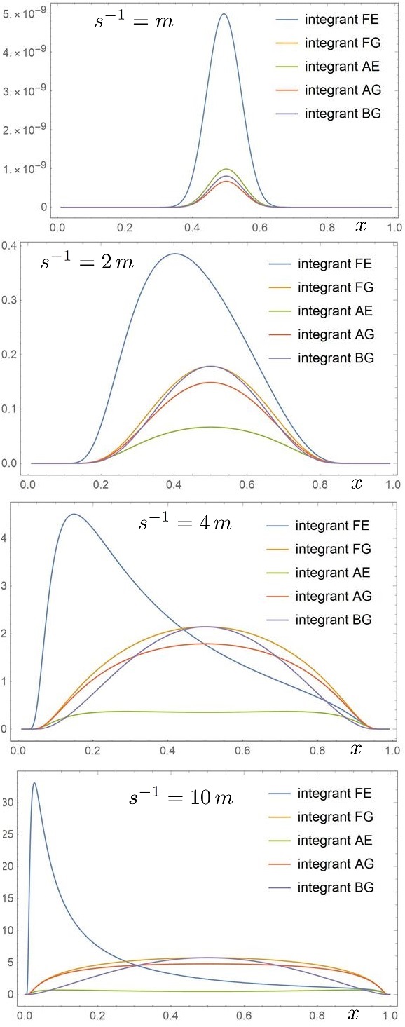
Figure 1: Five integrands of the integrals in Eqs. (146) to (150) that contribute to the fermion and boson effective masses, as indicated by their subscripts, for four values of the effective particle size $s$. The sequence shows how the integrands vary when the size $s$ is decreased. The coupling constant $\alpha_{g}=1/137$ and the gauge boson mass is set equal to the fermion mass, $\kappa=m$. The corresponding values of the mass corrections are given in Table 1.

For moderate values of $t$, the integrands of five integrals that contribute to the effective mass-squared corrections are plotted in Figs. 1 and 2. The purpose of these figures is to show the origin of characteristic behavior of the mass-squared corrections as functions of the size of effective particles. For simplicity of the presentation and later discussion of what happens when the boson mass decreases, we set in these figures the boson mass $\kappa$ equal to the fermion mass $m$. The corresponding values of mass-squared corrections, all in ratio to $m^{2}$, are listed in Table 1. We observe that the corrections are small for the size $s$ on the order of or greater than the Compton wavelength of fermions. The corrections grow quickly when $s$ decreases below the Compton wave length.

The fermion and transverse-boson (type $A$) mass-squared terms exhibit the dominant behavior $s^{-2}$. In contrast, the mass squared of longitudinal bosons (type $B$) is proportional to the physical value $\kappa^{2}$ and does not share with other quanta the rapid increase with $s^{-2}$. The fermion mass exhibits additional logarithmic increase with $s^{-2}$ due to the singular $x^{-1}$ behavior of the integral $I_{FE}$ for $x\to 0$, which is limited by the function erfc. The latter limits $x$ from below by a number order $s^{2}\kappa^{2}$, so the smaller $s$ the smaller allowed values of $x$ and the factor $1/x$ extends the support of fermion integrand toward $x=0$. In contrast, the boson mass integrands all behave symmetrically with respect to $x=1/2$. The difference between the fermion and boson integrands originates in the first-order Hamiltonian interaction term that causes a fermion to emit a boson, which includes the factor $\sim 1/\sqrt{x}$ that is squared in $\delta m^{2}$. The boson mass-squared correction comes from the interaction that produces a fermion-anti-fermion pair, in which no such $x$-dependent, fast growing factor arises.

Table 1: Values of mass corrections for equal boson and fermion masses, $\kappa=m$, and six values of the size $s$ of effective fermion and boson field quanta in units of the fermion Compton wavelength, according to Eqs. (143), (144) and (145) for $\alpha_{g}=1/137$. The entries correspond to the integrands shown in Figs. 1 and 2. These corrections cancel out with the effective particle self-interactions.

$s\,m$	$1$	$0.5$	$0.25$	$0.1$	$0.01$	$0.001$
$g^{2}\delta m^{2}/m^{2}$	$3.19\ 10^{-13}$	$3.03\ 10^{-4}$	$1.88\ 10^{-2}$	$3.67\ 10^{-1}$	$1.04\ 10^{2}$	$1.71\ 10^{4}$
$g^{2}\delta\kappa_{A}^{2}/m^{2}$	$2.73\ 10^{-13}$	$1.69\ 10^{-4}$	$5.17\ 10^{-3}$	$4.67\ 10^{-2}$	$4.85$	$4.85\ 10^{2}$
$g^{2}\delta\kappa_{B}^{2}/m^{2}$	$5.64\ 10^{-14}$	$3.38\ 10^{-5}$	$6.21\ 10^{-4}$	$1.96\ 10^{-3}$	$5.52\ 10^{-3}$	$9.09\ 10^{-3}$

In Fig. 2 the integrands are shown for values of $s$ hundred and thousand times smaller than the fermion Compton wavelength, approaching magnitudes comparable with the proton radius if the fermions have masses like electrons. The last two columns in Table 1 show how large the associated mass corrections become. The correction for fermions grows much faster with $s^{-1}$ than the correction for bosons $A$ does. The mass correction for bosons $B$ is much smaller than for bosons $A$ and exhibits also much smaller rate of increase with $s^{-1}$.

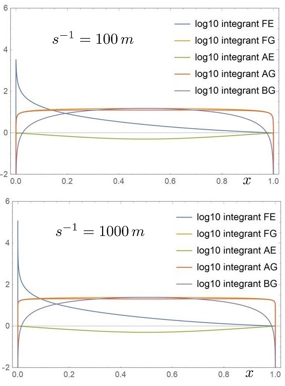
Figure 2: The five integrands of the integrals in Eqs. (146) to (150) as indicated by their subscripts for two much smaller values of the effective particle size $s$, necessarily in logarithmic scale, for all other parameters without change.

The large values of mass corrections for $\alpha_{g}=1/137$ may rise readers’ eyebrows. Indeed, such large values suggest that the perturbative expansion is under suspicion of inapplicability. However, the Hamiltonian $H_{t}$ leads to the self-interactions of effective particles that cancel the large mass-squared corrections. One may hope that such precise cancellation among large terms survives in the non-perturbative solutions of the eigenvalue equations similar to Eq. (95). Indeed, once the large terms order $s^{-2}\log{s\kappa}$ and $s^{-2}$ are canceled by the effective particle self-interaction and the remaining small parts are adjusted using eigenvalue equations for a single physical fermion and a single physical boson, the bound-state equation for the fermion-anti-fermion system is left with mass terms $m^{2}$ and $\kappa^{2}$ for all values of $t$. However, the warning that these results provide is that one needs a precise conceptual and quantitative control on the renormalized FF Hamiltonians, in order to describe binding of parton-like systems in gauge theories as well as one describes binding energies of constituents in spectroscopy of atomic systems.

In order to exhibit the actual magnitude of terms whose cancellation would have to be preserved, if one insisted on solving bound-state problems in canonical theory with some cutoff regularization that is meant to be lifted at the end of calculation, one can consider the gauge boson mass $\kappa=10^{-18}$ eV. This is the currently accepted experimental upper bound on the photon mass PDG . In the computation, one can set $\kappa=10^{-25}m$, imagining that $m$ could be the electron mass. On the basis of Figs. 1 and 2, one can foresee the result. It is illustrated in Fig. 3 in terms of the plots of three integrands as functions of $x$. Only three integrands are displayed because the remaining two are too small for showing them on the same figure. Instead, Table 2 provides the resulting mass-squared corrections themselves, in ratio to the physical fermion mass.

The fermion mass correction is much larger than the boson mass corrections. One can see that it is logarithmically sensitive to the lower bound on $x$, which is effectively set by the RGPEP form factor to be around $\sqrt{2}s^{2}\kappa^{2}$ divided by a number on the order of 100 or 1000. However, the dominant increase of the fermion mass correction is due to the factor $~{}s^{-2}$ that multiplies the logarithm. The factor $s^{-2}$ is due to the integration over large transverse momenta of a boson with respect to a fermion in the intermediate state in fermion self-interaction.

Boson masses behave differently. They do not exhibit the logarithmic behavior in $s$ that fermions do because the intermediate states of the boson self-interaction only consist of fermion-anti-fermion pairs. The pair mass is $10^{25}$ times larger than the boson mass and the boson mass correction varies mostly due to the spinor factors that after integration over transverse momenta render continuous and relatively slowly varying functions of $x$.

The intriguing feature of the boson mass corrections is that the types $A$ and $B$ are quite different, the latter being very small in comparison to the former. This result can be confronted with the expectation that in the limit of $\kappa\to 0$ the third-polarization boson decouples from fermions because the coupling is proportional to $\kappa$ Soper ; Yan3 . However, the actual coupling is of the form $\kappa/x$. Therefore, the small-$x$ behavior of the theory for $x$ order $s^{2}\kappa^{2}$ or smaller includes contributions from the bosons of type $B$. Only after the cancellation of small-$x$ singularities for finite $s$, the limit $\kappa\to 0$ can be considered in quantum theory.

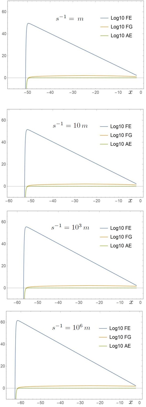
Figure 3: Three integrands of the integrals in Eqs. (146) to (148) for the boson mass much smaller than the fermion mass, $\kappa=10^{-25}\,m$ for four values of the effective particle size $s$. The figure illustrates behavior of the fermion integrand like $1/x$, where $x$ is the fraction of fermion momentum carried by the boson. Integrands in Eqs. (149) to (150) are relatively so small that they cannot be shown on the figure. The coupling constant $\alpha_{g}=1/137$. The corresponding values of the mass corrections for fermions and bosons are given in Table 1.

Concerning the magnitude of second-order mass corrections, we wish to state that in the case of constituent dynamics described by $H_{t}$ their values critically depend on the size of effective particles, see Tables 1 and 2. When the size of effective fermions increases toward and above their Compton wavelengths, the magnitude of corrections rapidly decreases. For example, the entries in Table 2 for $sm=2$ would be from top to bottom $3.95\ 10^{-2}$, $1.40\ 10^{-5}$ and an incredibly small $7.01\ 10^{-280}$. For $sm=4$, we obtain, correspondingly, $9.63\ 10^{-3}$, $1.05\ 10^{-6}$ and a number too small to quote. In Table 1, increasing $sm$ to 2 results in mass corrections of order $10^{-131}$. If the RGPEP tendency for mass stabilization when $s$ crosses the fermion Compton wavelength survives in advanced computations, the models of bound states based on a few-body Schroedinger picture with potentials and practically fixed effective constituent masses could be adopted as a leading approximation. In the next section, we describe behavior of the second-order relativistic potentials in a fermion-anti-fermion system.

Table 2: Values of mass corrections for the boson mass much smaller than the fermion mass, $\kappa=10^{-25}\,m$, in agreement with current experimental upper bound on the photon mass. Results for four values of the size $s$ of effective fermion and boson field quanta are shown in units of the fermion Compton wavelength, according to Eqs. (143), (144) and (145) for $\alpha=1/137$. The entries correspond to integrands shown in Fig. 3. These corrections cancel out with the effective particle self-interactions.

$s\,m$	$1$	$10^{-1}$	$10^{-3}$	$10^{-6}$
$g^{2}\delta m^{2}/m^{2}$	$1.62\ 10^{-1}$	$1.71\ 10^{+1}$	$1.85\ 10^{+5}$	$2.05\ 10^{+11}$
$g^{2}\delta\kappa_{A}^{2}/m^{2}$	$1.39\ 10^{-4}$	$4.93\ 10^{-2}$	$4.85\ 10^{+2}$	$4.85\ 10^{+8}$
$g^{2}\delta\kappa_{B}^{2}/m^{2}$	$3.17\ 10^{-70}$	$1.79\ 10^{-53}$	$8.92\ 10^{-53}$	$1.96\ 10^{-52}$

VI.2 Plots of relativistic potentials

The relativistic potentials for effective fermions of size $s$ are illustrated in this section by their action on wave functions of simple states. Consider a fermion-anti-fermion state described in terms of the parton-model variables. Let the fermions have equal momenta, so that they share their total momentum equally and their relative momentum is zero. To establish notation used for plotting potentials, this state of fermions is represented by

$$|1^{\prime}2^{\prime}\rangle = b_{t\,1^{\prime}}^{\dagger}d_{t\,2^{\prime}}^{\dagger}|0\rangle\ ,$$ (153)

where the individual momenta of fermions are $p_{1^{\prime}}=p_{2^{\prime}}=p^{\prime}$ and their total momentum is $P_{1^{\prime}2^{\prime}}=2p^{\prime}$. We use labels with primes as in Eq. (95), reserving the labels without primes for the states that result from action by the Hamiltonian. Thus, the plus and perpendicular components of fermions momenta are $p^{\prime+}=P_{1^{\prime}2^{\prime}}^{+}/2$ and $p^{\prime\perp}=P_{1^{\prime}2^{\prime}}^{\perp}/2$. In the FF dynamics, we can consider arbitrary values of the fermions total momentum components $P_{1^{\prime}2^{\prime}}^{+}$ and $P_{1^{\prime}2^{\prime}}^{\perp}$, while the individual fermions’ kinematic momentum components are always of the form given in Eqs. (107) and (109), in which $x^{\prime}=x_{1^{\prime}}=x_{2^{\prime}}=1/2$ and $k^{\prime\perp}=0$. The wave function $\psi_{t\,1^{\prime}2^{\prime}}$ in Eq. (95) that would correspond to the state $|1^{\prime}2^{\prime}\rangle$ would enforce with arbitrary accuracy that $(x^{\prime},k^{\prime\perp})=(1/2,0)$. We illustrate the relativistic potentials by results of their action on such wave functions.

We extract the relativistic potentials from the matrix elements $\langle 1_{t}2_{t}|H_{t\,{\rm eff}\,2\,q\bar{q}}|1^{\prime}_{t}2^{\prime}_{t}\rangle$ in Eq. (95) one-by-one in the order of lines $L_{1}$ to $L_{4}$ in Eq. (97). We remind the reader that the coupling constant is factored out. The potentials are functions of kinematic components of momenta of the two fermions that enter and two fermions that leave the interaction. Together, these are twelve arguments. But the total momentum of fermions is conserved and the potentials do not depend on it, no matter how large it is. So, they are functions of only six variables $x$, $k^{\perp}$, $x^{\prime}$ and $k^{\prime\perp}$. In action on the wave functions $\psi_{t\,1^{\prime}2^{\prime}}$ that we introduced above, the primed variables have fixed values $x^{\prime}=1/2$ and $k^{\prime\perp}=0$. In addition, as a consequence of rotational symmetry around $z$-axis and $k^{\prime\perp}$ being zero, the result of action of a potential depends only on the variables $x$ and $k^{\perp 2}$. We denote

$$Q = |k^{\perp}|\ .$$ (154)

This way we obtain four functions $V_{1}(x,Q)$ to $V_{4}(x,Q)$ from the potentials $V_{1}(121^{\prime}2^{\prime})$ to $V_{4}(121^{\prime}2^{\prime})$ in Eqs. (119), (127), (135) and (137), so that for $i=1$, 2, 3 and 4 we have

$$V_{i}(x,Q) = V_{i}(12p^{\prime}p^{\prime})\ .$$ (155)

These functions are plotted in comparison with two reference functions defined below. The reference functions correspond to the intuitive potentials that apply in non-relativistic quantum mechanics.

The first reference function is defined using the momentum representation of the attractive Yukawa potential in non-relativistic quantum mechanics, which reads

$$V_{Y}(\vec{k},\vec{k}\,^{\prime}) = {-g^{2}\over(\vec{k}-\vec{k}\,^{\prime})^{2}+\kappa^{2}}\ .$$ (156)

Since the relative momentum in the state $|1^{\prime}2^{\prime}\rangle$ that we use is zero, one sets $\vec{k}\,^{\prime}$ to zero. The argument of the Yukawa non-relativistic potential reduces to $\vec{k}\,^{2}$. We identify the non-relativistic $\vec{k}$ with its FF counterpart using formulas of App. A,

$$\vec{k}\,^{2} = {\cal M}_{12}^{2}/4-m^{2}\,=\,{Q^{2}+[(x-1/2)2m]^{2}\over 4x(1-x)}\ .$$ (157)

In the non-relativistic limit the denominator $4x(1-x)$ turns into 1. Therefore, the Yukawa potential function we could use as a reference would be

$${-g^{2}\over Q^{2}+[(x-1/2)2m]^{2}+\kappa^{2}}\ .$$ (158)

However, in lines $L_{1}$ to $L_{4}$ we have factored out spinor matrix elements and the square of the coupling constant with proper signs. Our Yukawa reference function is therefore defined to be

$$V_{Y}(x,Q) = {4m^{2}\over Q^{2}+[(x-1/2)2m]^{2}+\kappa^{2}}\ .$$ (159)

For small $\kappa/m$, the maximal value of this function equals $4m^{2}/\kappa^{2}$ and the minimal one is zero.

Our second reference function is designed for the annihilation channel potentials. We strip the RGPEP form factor from the potential $V_{3}$ in Eq. (135) and obtain

$$2m^{2}\left({1\over b}+{1\over b^{\prime}}\right)$$ (160)

with $b={\cal M}_{12}^{2}-\kappa^{2}$ and $b^{\prime}=4m^{2}-\kappa^{2}$. Our annihilation reference function is hence defined to be

$$V_{A}(x,Q) = 2m^{2}\ \left[{x(1-x)\over Q^{2}+m^{2}-\kappa^{2}x(1-x)}+{1\over 4m^{2}-\kappa^{2}}\right]\ .$$ (161)

Its maximal value is one and it tends to 1/2 for large values of $Q$ or extreme values of $x$, when $\kappa\ll m$.

In all figures that illustrate the relativistic potentials, we use the same boson mass $\kappa=m/7$ and the same size of effective particles $s=(1.5\,m)^{-1}$. These choices are made for purely graphical reasons, to satisfy the condition that the characteristic features of the interactions are visible well. When the mass $\kappa$ decreases, the Yukawa potential at small momentum transfers becomes increasingly spiky and approximates the Coulomb potential near $x=1/2$ and $Q=0$ increasingly well. For the parameters chosen in the figures, the Yukawa-like potentials reach the value $4m^{2}/\kappa^{2}=196$, see Eq. (159). When the size $s$ increases, the potentials lose strength off shell, which means they are exponentially limited to a smaller range of $x$ and $Q$. When $s$ decreases, the range increases according to the rule $[Q^{2}+m^{2}(2x-1)^{2}]/[x(1-x)]\lesssim s^{-2}$.

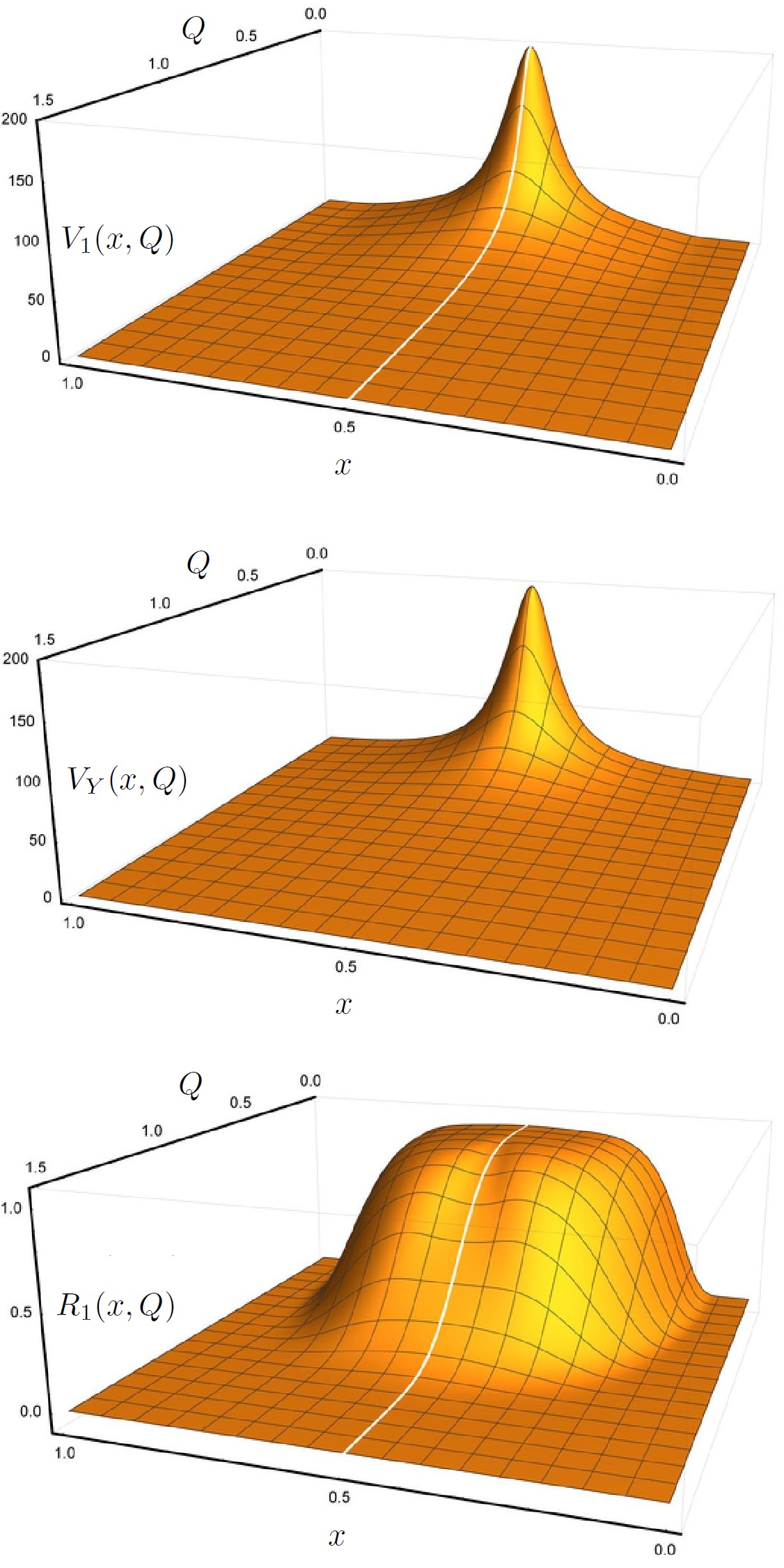
Figure 4: Relativistic gauge-boson exchange potential $V_{1}(121^{\prime}2^{\prime})$ of Eq. (119). The upper plot illustrates $V_{1}(121^{\prime}2^{\prime})$ in terms of the potential function $V_{1}(x,Q)$ of Eq. (155). For graphical reasons, the boson mass $\kappa$ is set to one seventh of the fermion mass $m$ and the RGPEP running size parameter $s$ to the inverse of $1.5\,m$. The variable $x$ corresponds to the parton-model $x$ of the fermion labeled by 1. The variable $Q$ is the magnitude of transverse momentum of that fermion with respect to the anti-fermion labeled by 2. The middle panel shows the Yukawa potential function $V_{Y}(x,Q)$ of Eq. (159), hardly discernible from $V_{1}(x,Q)$. The bottom figure presents the ratio $R_{1}(x,Q)=V_{1}(x,Q)/V_{Y}(x,Q)$ of Eq. (162). The ratio exhibits the exponential suppression of effective interactions when the invariant mass changes by more than the inverse of the RGPEP scale parameter $s$. More details are in the text.

Figure 4 contains three panels that show, counting from the top to bottom, the boson exchange potential function $V_{1}(x,Q)$ of Eq. (119), the Yukawa potential function $V_{Y}(x,Q)$ of Eq. (159) and their ratio

$$R_{1}(x,Q) = V_{1}(x,Q)/V_{Y}(x,Q)\ .$$ (162)

These figures demonstrate the role of the RGPEP form factors in effective interactions. The form factors exponentially suppress the interactions that change the effective fermions invariant mass by more than the inverse of an effective fermion size $s$. While the relativistic potential function $V_{1}(x,Q)$ appears almost indistinguishable from the Yukawa potential function $V_{Y}(x,Q)$, their ratio displays a huge difference from one, due to the RGPEP form factors. In the figures, fermions 1’ and 2’ have the invariant mass squared equal ${\cal M}^{\prime 2}=4m^{2}$. Fermions 1 and 2 have the invariant mass squared equal ${\cal M}^{2}=(Q^{2}+m^{2})/[x(1-x)]$. Generally, the RGPEP form factors exponentially suppress the interactions off-shell extent according to the rule $({\cal M}^{2}-{\cal M}^{\prime 2})\lesssim s^{-2}$. When the variable $x^{\prime}$ introduced below Eq. (153) deviates from 0.5, the Yukawa peak of Fig. 4 shifts and centers on $x=x^{\prime}$ instead of 0.5. If the transverse momentum $k^{\prime\perp}$ significantly differs from zero, the potential function behaves in a somewhat more complicated way due to its additional dependence on $x^{\prime}$, $Q^{\prime}$ and the angle between $k^{\perp}$ and $k^{\prime\perp}$ in the transverse plane, but it follows the rule that $(Q^{2}+m^{2})/[x(1-x)]$ does not differ from $(Q^{\prime 2}+m^{2})/[x^{\prime}(1-x^{\prime})]$ by much more than $1/s^{2}$.

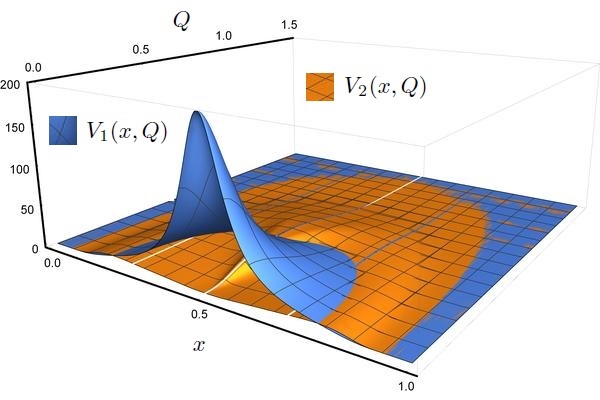
Figure 5: Relativistic potential $V_{2}(121^{\prime}2^{\prime})$ of Eq. (127). It is drawn in terms of the potential function $V_{2}(x,Q)$ of Eq. (155), in orange. For comparison, the Yukawa-like potential function $V_{1}(x,Q)$ of Eq. (155), see Fig. 4, is shown in blue. The functions are displayed with the same sign to show their relative magnitudes well. The view of potentials is arranged to be from the opposite point to that in Fig. 4 in order to show the relative magnitude of the two functions at small momentum transfers, which is the region where the bound-state formation mechanism is most active. In that region, the potential function $V_{2}(x,Q)$ is much smaller in size than the Yukawa-like function $V_{1}(x,Q)$. The Yukawa peak reaches $4\times 49$, as explained below Eq. (159). The potential function $V_{2}(x,Q)$ vanishes at that point.

Figure 5 shows the relativistic FF potential of Eq. (127) in terms of the function $V_{2}(x,Q)$ in Eq. (155), in comparison with the potential function $V_{1}(x,Q)$, shown in Fig. 4 for the same parameters $\kappa$ and $s$. It is visible that the relativistic FF potential $V_{2}(121^{\prime}2^{\prime})$ has support only off shell. In the region of binding, it is very small in comparison to the one-boson-exchange potential $V_{1}(121^{\prime}2^{\prime})$. In the language of SRG GlazekWilson , it has significant matrix elements only outside the band of a band-diagonal matrix of the effective Hamiltonian, whose width in terms of the invariant mass is $1/s$. Far away from the diagonal, the function $V_{2}(x,Q)$ briefly exceeds the function $V_{1}(x,Q)$, where the latter is already two orders of magnitude smaller than in the band. This partial dominance of $V_{2}(x,Q)$ over $V_{1}(x,Q)$ is the origin of the huff-like pattern visible in Fig. 5.

The potential $V_{2}$ does not contribute to the on-shell scattering matrix in the Born approximation and does not have a classical counterpart, in contrary to the potential $V_{1}$ that corresponds to the Yukawa potential. This is a welcome feature because the potential $V_{2}$ multiplies the non-covariant spin structure $EX_{+}$ of Eq. (103), see Eq. (126). The factor $EX_{+}$ preserves spins of fermions and introduces the factor $\sqrt{x(1-x)x^{\prime}(1-x^{\prime})}$ that further suppresses the interaction for extreme values of $x$ or $x^{\prime}$. The alien feature of $V_{2}(x,Q)$ near $x=1/2$ originates from the factor $1/(x-x^{\prime})$ that produces a discontinuous variation of the potential as a function of $x$ for $x^{\prime}\neq 1/2$. The discontinuity is suppressed by additional powers of $x-1/2$ for $x^{\prime}=1/2$. For $x^{\prime}\neq 1/2$, it is integrable with regular wave functions of $x$ and $x^{\prime}$ in the sense of principal value.

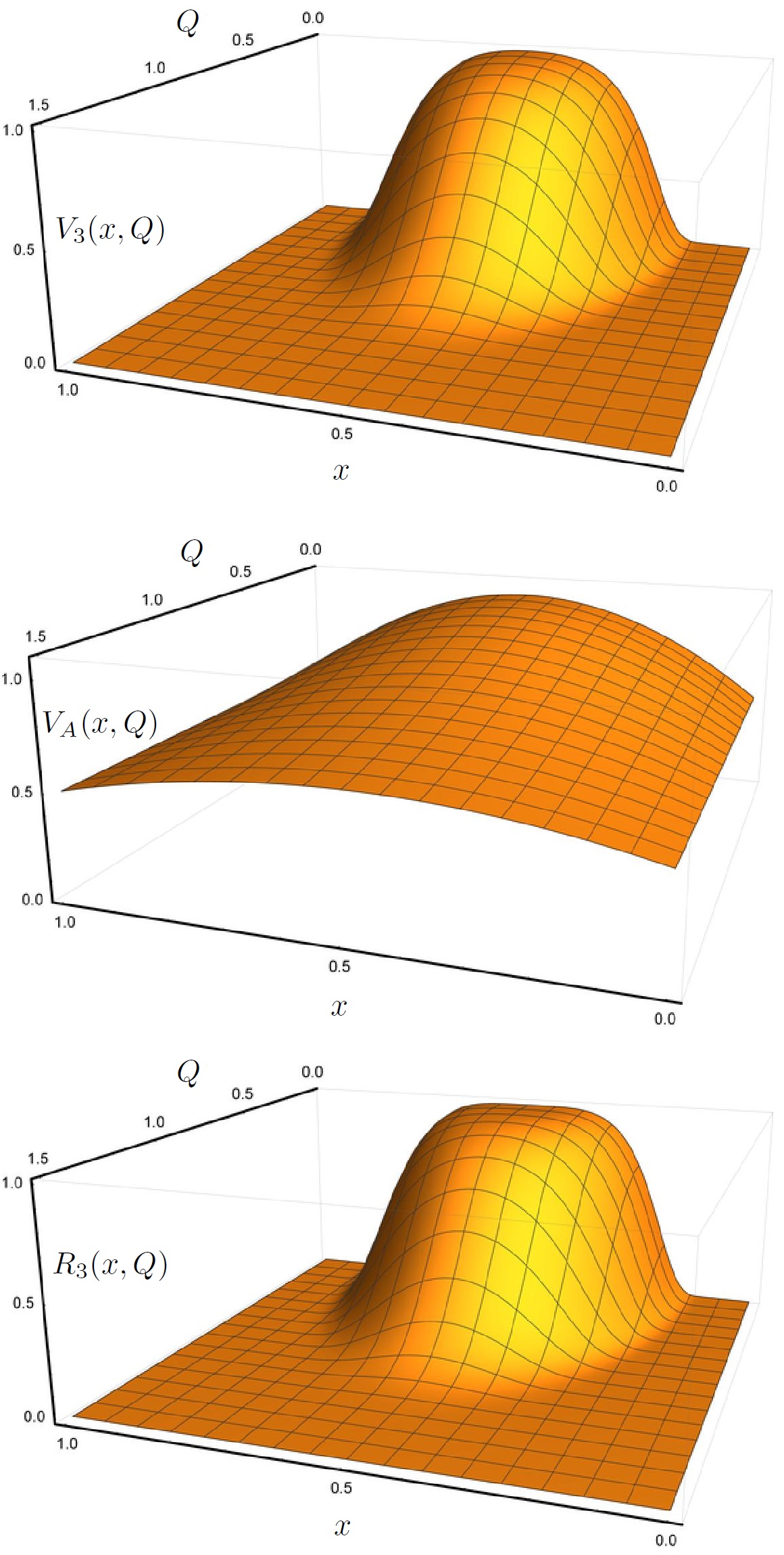
Figure 6: Relativistic annihilation-channel potential $V_{3}(121^{\prime}2^{\prime})$ of Eq. (135), shown in terms of the potential function $V_{3}(x,Q)$ of Eq. (155). One sees the effect of the RGPEP form factors. The middle panel shows the annihilation-channel potential function $V_{A}(x,Q)$ of Eq. (161). The ratio $R_{3}(x,Q)=V_{3}(x,Q)/V_{A}(x,Q)$ is shown in the bottom panel, see the text.

Figure 6 shows three panels that, counting from the top to botom, illustrate the boson annihilation channel potential function $V_{3}(121^{\prime}2^{\prime})$ of Eq. (135). The top panel shows the function $V_{3}(x,Q)$ of Eq. (155). The middle panel shows the potential function $V_{A}(x,Q)$ of Eq. (161). The ratio $R_{3}(x,Q)=V_{3}(x,Q)/V_{A}(x,Q)$ is shown in the bottom panel. Comparing the panels top with middle, one sees again the role of the RGPEP form factors. In the SRG language, they squeeze the potential to the band of effective theory. The bottom-panel ratio function $R_{3}(x,Q)$ is characterized by a little more flat shape than the top panel potential function $V_{3}(x,Q)$. This effect shows that the RGPEP form factor introduces a relativistic annihilation-channel potential that is close to the function $V_{A}(x,Q)$ times the RGPEP form factor.

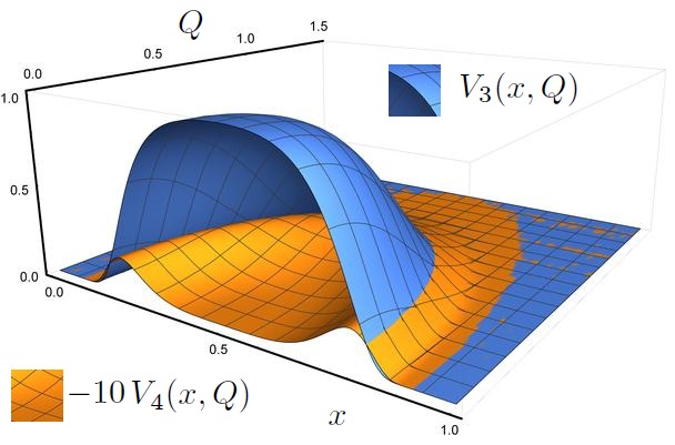
Figure 7: Relativistic annihilation-channel potential functions $-10\,V_{4}(x,Q)$ and $V_{3}(x,Q)$. See the text for details.

Finally, Fig. 7 illustrates the relativistic FF annihilation-channel potential $V_{4}(121^{\prime}2^{\prime})$ of Eq. (137) in terms of the potential function $V_{4}(x,Q)$ in Eq. (155), shown simultaneously with the potential function $V_{3}(x,Q)$ of Eq. (155). The comparison shows the smallness of $V_{4}(x,Q)$. Its sign is changed and its value is multiplied by ten in order to obtain an informative picture. The relativistic potential $V_{4}(121^{\prime}2^{\prime})$ appears in the line $L_{4}$ in Eq. (136) multiplied by the frame-dependent spin factor $AN_{+}$ of Eq. (105). It does not contribute to the on-shell scattering matrix in the Born approximation and does not have any familiar counterpart in quantum mechanics. However, it does participate in the off-shell bound-state dynamics, in addition to the potential $V_{3}$. Its significance in that dynamics is not known at this point. The actual magnitude of the boson mass $\kappa$ much smaller than the fermion mass $m$, does not influence the potentials $V_{3}$ and $V_{4}$ in any significant way.

VII Conclusion

The RGPEP allows one to calculate second-order effective masses and interactions in the fermion-anti-fermion systems in Abelian gauge theory. Canonical Hamiltonian leads to difficulties with unambiguous handling of small $x$ and large $k^{\perp}$ singularities because the singular terms involve the ratio $k^{\perp 2}/x$ and the ultraviolet divergences are mixed with the small $x$ divergences. As a result, the ultraviolet counter terms involve unknown functions of $x$ and small-$x$ counter terms contain functions of $k^{\perp}$ Wilsonetal . However, once the mass parameter for gauge bosons is introduced according to the principles of local gauge symmetry and spontaneous violation of the global gauge symmetry, a mass gap is introduced and one achieves unambiguous control on the divergences. The ultraviolet, small-$x$ and infrared singularities are separated from each other in a way specific to the FF Hamiltonian dynamics and the RGPEP evolution of Hamiltonian operators. Namely, the longitudinal small-$x$ region is controlled by the parameter $s\kappa$ while the transverse ultraviolet region is controlled by $s$, where $s$ is the RGPEP a priori arbitrary scale parameter. The origin of the separation lies in the expression

$$s^{2}\delta{\cal M}^{2} = {(s\kappa)^{2}+(sk^{\perp})^{2}\over x}$$ (163)

for the contribution of bosons to the arguments of exponentially falling-off RGPEP form factors in the effective interactions. It is visible that one cannot make $s^{2}{\cal M}^{2}$ small for small $x$ by making $sk^{\perp}$ small because eventually $s\kappa$ begins to count and $s{\cal M}$ always diverges for fixed $s$ when $x\to 0$.

Using expansion in the coupling constant $g$, one can employ the RGPEP to study what happens when the boson mass $\kappa$ is varied and what comes out in terms of the effective theory when $\kappa$ is made very small. The result of second-order calculations described in this article is that the fermion mass counter terms can reach enormous values. Their contribution is canceled precisely in the second-order mass eigenvalue equation for physical fermions or bosons, but the canceled terms are much greater than the eigenvalues, if the size of effective quanta is very small. However, when that size is increased toward the fermions Compton wavelength and above, the mass corrections become very small.

It is also found that the effective boson masses vary differently with the size $s$ for the commonly known transverse bosons and for the less known longitudinal ones. The mass corrections for the latter stay small or very small in comparison to the mass corrections for the former.

The RGPEP also allows one to calculate interaction terms that drive the fermion-anti-fermion bound state dynamics. One obtains Yukawa potentials that tend to the Coulomb potential when the boson mass tends to zero and the size of effective quanta increases to and above the fermion Compton wavelength. However, the size increase is associated with development of increasingly important vertex form factors that suppress interactions with large changes of the invariant mass of fermions.

The fact that the FF Hamiltonian dynamics is invariant with respect to the Lorentz boosts along one axis, besides six other Poincaré transformations, allows one to relate the RGPEP results for the Coulomb- or Yukawa-like systems to their parton model picture. The results described in this article suggest that when we imagine partons as constituents, their size cannot be ignored. If one ignores their size, the power-like behavior of perturbative interactions is extended to the phase-space region where the eigenvalue condition for bound states imposes decisive departures of the wave functions from their perturbative estimates that use canonical interactions. The effective interactions become exponentially suppressed when the fermions invariant mass changes by more than the inverse of their Compton wavelength. One also obtains small effective interaction terms that appear in addition to the Coulomb and Yukawa potentials and do not have classical counterparts. The RGPEP enables us to draw details of all these potentials.

It is not clear what happens in the higher order RGPEP calculations. Of key interest is the fourth order. This is where the running of effective coupling constant shows up in the bound-state dynamics for the first time. The computation is certainly doable and the results would be of interest.

The final question we wish to address is whether Soper’s theory is a valid approximation to the gauge theory with spontaneously broken global symmetry. We obtain the former from the latter in the massive limit in which the classical field $h/v$ is set to zero when $v$ is formally sent to infinity. However, the limit is considered in a classical Lagrangian. The effective quantum theory derived using the RGPEP will include corrections that depend on the momentum range $1/s_{r}$ of interactions in ratio to $v$. The order of limits $v\to\infty$ and $s_{r}\to 0$ may matter. At this point, the calculations described here are considered reasonable regarding gauge symmetry because they are carried out using the massive limit that results in the Soper theory, which by itself is an example of a theory with a form of gauge symmetry. The full theory, not using the massive limit, can also be analyzed using the RGPEP.

Appendix A Notation

Translation invariance on the front implies conservation of momentum described by the $\delta$-function $\tilde{\delta}_{c.a}$, where $c$ denotes created and $a$ annihilated quanta. We use the convention

$$\tilde{\delta}_{c.a} = 2(2\pi)^{3}\delta(P_{c}^{+}-P_{a}^{+})\delta^{2}(P_{c}^{\perp}-P_{a}^{\perp})\ ,$$ (164)

where $P_{c}$ and $P_{a}$ denote the total momenta of particles created and annihilated, respectively. The corresponding invariant masses are ${\cal M}_{c}^{2}=P_{c}^{2}$ and ${\cal M}_{a}^{2}=P_{a}^{2}$ with minus components of individual particles momenta calculated from their mass shell conditions, $p^{-}=(m^{2}+p^{\perp 2})/p^{+}$.

Integration over a single particle phase space,

$$\int d^{4}p\ \delta(p^{2}-m^{2})\ \theta(p^{0}) = \int{d^{3}p\over 2E_{p}}\,=\,\int_{0}^{\infty}{dp^{+}\over 2p^{+}}\int d^{2}p^{\perp}\ ,$$ (165)

is denoted by $\int[p]$ and if one has more particles to integrate over their momenta $p_{1}$, $p_{2}$, . . . $p_{n}$, the integral is abbreviated to

$$\int[12...n] = \int[p_{1}]\int[p_{2}]...\int[p_{n}]\ .$$ (166)

When two particles have together momentum $P$ and carry fractions $x$ and $1-x$ of it and some transverse relative momentum $k^{\perp}$,

$$p_{1}^{+} = xP^{+}\ ,$$ (167)

$$p_{2}^{+} = (1-x)P^{+}\ ,$$ (168)

$$p_{1}^{\perp} = xP^{\perp}+k^{\perp}\ ,$$ (169)

$$p_{2}^{\perp} = (1-x)P^{\perp}-k^{\perp}\ ,$$ (170)

one has

$$\int[12] = \int[P]\int[xk]\ ,$$ (171)

$$\int[xk] = \int_{0}^{1}{dx\over 4\pi x(1-x)}\int{d^{2}k^{\perp}\over(2\pi)^{2}}\ .$$ (172)

In terms of the relative three-momentum of two particles of mass $m$ in their rest frame, $\vec{k}$,

$$x = (1+k_{z}/E_{k})/2\ ,$$ (173)

$${dx\over x(1-x)} = {2\ dk_{z}\over E_{k}}\ ,$$ (174)

$$\int[xk] = \int{d^{3}k\over(2\pi)^{3}E_{k}}\ ,$$ (175)

where $E_{k}=\sqrt{m^{2}+\vec{k}\,^{2}}$. The invariant mass of two particles is

$$(p_{1}+p_{2})^{2} = (p_{1}^{+}+p_{2}^{+})(p_{1}^{-}+p_{2}^{-})-(p_{1}^{\perp}+p_{2}^{\perp})^{2}$$ (176)

$$= {k^{\perp 2}+m_{1}^{2}\over x}+{k^{\perp 2}+m_{2}^{2}\over 1-x}$$ (177)

$$= \left(\sqrt{m_{1}^{2}+\vec{k}\,^{2}}+\sqrt{m_{2}^{2}+\vec{k}\,^{2}}\right)^{2}\ .$$ (178)

We use spinors $u_{p\sigma}=B(p,m)u_{\sigma}$ and $v_{p\sigma}=B(p,m)v_{\sigma}$ in which the spinors at rest are related by $v_{\sigma}=Cu^{*}_{\sigma}$ with $C=i\gamma^{2}$ and the front boost matrix is $B(p,m)={1\over\sqrt{p^{+}m}}[\Lambda_{+}p^{+}+\Lambda_{-}(m+p^{\perp}\alpha^{\perp})]$, where $\Lambda_{\pm}={1\over 2}(1\pm\alpha^{3})$. The spinors at rest are

$$u_{\sigma} = \sqrt{2m}\left[\begin{array}[]{c}\chi_{\sigma}\\ 0\end{array}\right]\ ,\quad v_{\sigma}\,=\,\sqrt{2m_{f}}\left[\begin{array}[]{c}0\\ \xi_{-\sigma}\end{array}\right]\ ,$$ (183)

where $\xi_{-\sigma}=-i\sigma_{2}\chi_{\sigma}=\sigma\chi_{-\sigma}$, cf. LepageBrodsky ; fermions . Free bosons of type $A$ have polarization vectors

$$\varepsilon^{\mu}_{p\sigma} = \left(\varepsilon^{-}_{p\sigma}=2p^{\perp}\varepsilon^{\perp}_{\sigma}/p^{+},\varepsilon^{\perp}_{\sigma}\right)$$ (184)

with $\varepsilon^{\perp}_{\sigma}=(1+\sigma,1-\sigma)/2$. Free bosons of type $B$ have polarization vectors

$$\varepsilon_{p3} = \left(\varepsilon_{p3}^{-}={p^{\perp\,2}-\kappa^{2}\over\kappa p^{+}},~{}\varepsilon_{p3}^{+}={p^{+}\over\kappa},~{}\varepsilon_{p3}^{\perp}={p^{\perp}\over\kappa}\right)$$ (185)

$$= {p\over\kappa}-\eta{\kappa\over p^{+}}\ ,$$ (186)

and $\eta^{+}=\eta^{\perp}=0$ while $\eta^{-}=2$.

Appendix B Details of the initial Hamiltonian

The canonical Hamiltonian terms in Eq. (39) are listed below using notation explained in App. A. The subscript 0 associated with canonical creation and annihilation operators for the bare quanta that are considered point-like, or of size $s_{r}=t_{r}^{1/4}\to 0$ as the regularization is being lifted, is not needed here and it is omitted. The free part of the Hamiltonian is $H_{f}=H_{\psi^{2}}+H_{A^{2}}+H_{B^{2}}$, where

$$H_{\psi^{2}} = \sum_{\sigma=1}^{2}\int[p]{p^{\perp\,2}+m^{2}\over p^{+}}\left[b^{\dagger}_{p\sigma}b_{p\sigma}+d^{\dagger}_{p\sigma}d_{p\sigma}\right]\ ,$$ (187)

$$H_{A^{2}} = \sum_{\sigma=1}^{2}\int[p]{p^{\perp\,2}+\kappa^{2}\over p^{+}}a^{\dagger}_{p\sigma}a_{p\sigma}\ ,$$ (188)

$$H_{B^{2}} = \int[p]{p^{\perp\,2}+\kappa^{2}\over p^{+}}c^{\dagger}_{p}c_{p}\ .$$ (189)

The interaction Hamiltonian $H_{I}=H-H_{f}$ contains terms of orders $g$ and $g^{2}$. The terms order $g$ are

$$H_{\psi A\psi} = g\sum_{123}\int[123]\,\tilde{\delta}_{c.a}\,\left[\bar{u}_{2}\not\!\varepsilon_{1}^{*}u_{3}\ b^{\dagger}_{2}a^{\dagger}_{1}b_{3}-\bar{v}_{3}\not\!\varepsilon_{1}^{*}v_{2}\ d^{\dagger}_{2}a^{\dagger}_{1}d_{3}+\bar{u}_{1}\not\!\varepsilon_{3}v_{2}\ b^{\dagger}_{1}d^{\dagger}_{2}a_{3}\ +\ h.c.\right]\ ,$$ (190)

$$H_{\psi B\psi} = -g\sum_{12}\int[123]\,\tilde{\delta}_{c.a}\,\left[\bar{u}_{2}{\kappa\gamma^{+}\over p_{1}^{+}}u_{3}\ b^{\dagger}_{2}c^{\dagger}_{1}b_{3}-\bar{v}_{3}{\kappa\gamma^{+}\over p_{1}^{+}}v_{2}\ d^{\dagger}_{2}c^{\dagger}_{1}d_{3}+\bar{u}_{1}{\kappa\gamma^{+}\over p_{3}^{+}}v_{2}\ b^{\dagger}_{1}d^{\dagger}_{2}c_{3}\ +\ h.c.\right]\ .$$ (191)

There are two terms order $g^{2}$. The term due to constraint on $\psi_{-}$ is

$$H_{\psi AA\psi} = {g^{2}\over 2}\sum_{1234}\int[1234]\,\tilde{\delta}_{c.a}\,\left\{~{}\right\}_{\psi AA\psi}\ ,$$ (192)

where, in the universal order $b^{\dagger}d^{\dagger}a^{\dagger}adb$,

$$\left\{~{}\right\}_{\psi AA\psi} = {\bar{u}_{1}\not\!\varepsilon_{2}^{*}\gamma^{+}\not\!\varepsilon_{3}u_{4}\over p_{3}^{+}+p_{4}^{+}}\ b_{1}^{\dagger}a_{2}^{\dagger}a_{3}b_{4}+{\bar{u}_{1}\not\!\varepsilon_{2}^{*}\gamma^{+}\not\!\varepsilon_{3}v_{4}\over p_{3}^{+}-p_{4}^{+}}\ b_{1}^{\dagger}d_{4}^{\dagger}a_{2}^{\dagger}a_{3}+{\bar{u}_{1}\not\!\varepsilon_{2}^{*}\gamma^{+}\not\!\varepsilon_{3}^{*}u_{4}\over p_{4}^{+}-p_{3}^{+}}\ b_{1}^{\dagger}a_{2}^{\dagger}a_{3}^{\dagger}b_{4}$$ (193)

$$+ {\bar{u}_{1}\not\!\varepsilon_{2}\gamma^{+}\not\!\varepsilon_{3}u_{4}\over p_{3}^{+}+p_{4}^{+}}\ b_{1}^{\dagger}a_{2}a_{3}b_{4}+{\bar{u}_{1}\not\!\varepsilon_{2}\gamma^{+}\not\!\varepsilon_{3}v_{4}\over p_{3}^{+}-p_{4}^{+}}\ b_{1}^{\dagger}d_{4}^{\dagger}a_{2}a_{3}+{\bar{u}_{1}\not\!\varepsilon_{2}\gamma^{+}\not\!\varepsilon_{3}^{*}u_{4}\over p_{4}^{+}-p_{3}^{+}}\ b_{1}^{\dagger}a_{3}^{\dagger}a_{2}b_{4}-{\bar{u}_{1}\not\!\varepsilon_{2}\gamma^{+}\not\!\varepsilon_{3}^{*}v_{4}\over p_{3}^{+}+p_{4}^{+}}\ b_{1}^{\dagger}d_{4}^{\dagger}a_{3}^{\dagger}a_{2}$$

$$+ {\bar{v}_{1}\not\!\varepsilon_{2}^{*}\gamma^{+}\not\!\varepsilon_{3}u_{4}\over p_{3}^{+}+p_{4}^{+}}\ a_{2}^{\dagger}a_{3}d_{1}b_{4}+{\bar{v}_{1}\not\!\varepsilon_{2}^{*}\gamma^{+}\not\!\varepsilon_{3}v_{4}\over p_{4}^{+}-p_{3}^{+}}\ d_{4}^{\dagger}a_{2}^{\dagger}a_{3}d_{1}+{\bar{v}_{1}\not\!\varepsilon_{2}^{*}\gamma^{+}\not\!\varepsilon_{3}^{*}u_{4}\over p_{4}^{+}-p_{3}^{+}}\ a_{2}^{\dagger}a_{3}^{\dagger}d_{1}b_{4}+{\bar{v}_{1}\not\!\varepsilon_{2}^{*}\gamma^{+}\not\!\varepsilon_{3}^{*}v_{4}\over p_{3}^{+}+p_{4}^{+}}\ d_{4}^{\dagger}a_{2}^{\dagger}a_{3}^{\dagger}d_{1}$$

$$+ {\bar{v}_{1}\not\!\varepsilon_{2}\gamma^{+}\not\!\varepsilon_{3}v_{4}\over p_{4}^{+}-p_{3}^{+}}\ d_{4}^{\dagger}a_{2}a_{3}d_{1}+{\bar{v}_{1}\not\!\varepsilon_{2}\gamma^{+}\not\!\varepsilon_{3}^{*}u_{4}\over p_{4}^{+}-p_{3}^{+}}\ a_{3}^{\dagger}a_{2}d_{1}b_{4}+{\bar{v}_{1}\not\!\varepsilon_{2}\gamma^{+}\not\!\varepsilon_{3}^{*}v_{4}\over p_{3}^{+}+p_{4}^{+}}\ d_{4}^{\dagger}a_{3}^{\dagger}a_{2}d_{1}\ .$$

The term due to constraint on $A^{-}$ is

$$H_{(\psi\psi)^{2}} = {g^{2}\over 2}\sum_{1234}\int[1234]\,\tilde{\delta}_{c.a}\,\left\{~{}\right\}_{(\psi\psi)^{2}}\ ,$$ (194)

where $\left\{~{}\right\}_{(\psi\psi)^{2}}$ reads

$$\left\{~{}\right\}_{(\psi\psi)^{2}} = -{\bar{u}_{1}\gamma^{+}u_{2}\ \bar{u}_{3}\gamma^{+}u_{4}\over(p_{3}^{+}-p_{4}^{+})^{2}}\ b_{1}^{\dagger}b_{3}^{\dagger}b_{2}b_{4}+{\bar{u}_{1}\gamma^{+}u_{2}\ \bar{u}_{3}\gamma^{+}v_{4}\over(p_{3}^{+}+p_{4}^{+})^{2}}\ b_{1}^{\dagger}b_{3}^{\dagger}d_{4}^{\dagger}b_{2}$$ (195)

$$- {\bar{u}_{1}\gamma^{+}u_{2}\ \bar{v}_{3}\gamma^{+}u_{4}\over(p_{3}^{+}+p_{4}^{+})^{2}}\ b_{1}^{\dagger}d_{3}b_{2}b_{4}-{\bar{u}_{1}\gamma^{+}u_{2}\ \bar{v}_{3}\gamma^{+}v_{4}\over(p_{3}^{+}-p_{4}^{+})^{2}}\ b_{1}^{\dagger}d_{4}^{\dagger}d_{3}b_{2}$$

$$- {\bar{u}_{1}\gamma^{+}v_{2}\ \bar{u}_{3}\gamma^{+}u_{4}\over(p_{3}^{+}-p_{4}^{+})^{2}}\ b_{1}^{\dagger}b_{3}^{\dagger}d_{2}^{\dagger}b_{4}$$

$$+ {\bar{u}_{1}\gamma^{+}v_{2}\ \bar{v}_{3}\gamma^{+}u_{4}\over(p_{3}^{+}+p_{4}^{+})^{2}}\ b_{1}^{\dagger}d_{2}^{\dagger}d_{3}b_{4}-{\bar{u}_{1}\gamma^{+}v_{2}\ \bar{v}_{3}\gamma^{+}v_{4}\over(p_{3}^{+}-p_{4}^{+})^{2}}\ b_{1}^{\dagger}d_{2}^{\dagger}d_{4}^{\dagger}d_{3}$$

$$+ {\bar{v}_{1}\gamma^{+}u_{2}\ \bar{u}_{3}\gamma^{+}u_{4}\over(p_{3}^{+}-p_{4}^{+})^{2}}\ b_{3}^{\dagger}d_{1}b_{2}b_{4}+{\bar{v}_{1}\gamma^{+}u_{2}\ \bar{u}_{3}\gamma^{+}v_{4}\over(p_{3}^{+}+p_{4}^{+})^{2}}\ b_{3}^{\dagger}d_{4}^{\dagger}d_{1}b_{2}$$

$$+ {\bar{v}_{1}\gamma^{+}u_{2}\ \bar{v}_{3}\gamma^{+}v_{4}\over(p_{3}^{+}-p_{4}^{+})^{2}}\ d_{4}^{\dagger}d_{1}d_{3}b_{2}$$

$$- {\bar{v}_{1}\gamma^{+}v_{2}\ \bar{u}_{3}\gamma^{+}u_{4}\over(p_{3}^{+}-p_{4}^{+})^{2}}\ b_{3}^{\dagger}d_{2}^{\dagger}d_{1}b_{4}+{\bar{v}_{1}\gamma^{+}v_{2}\ \bar{u}_{3}\gamma^{+}v_{4}\over(p_{3}^{+}+p_{4}^{+})^{2}}\ b_{3}^{\dagger}d_{2}^{\dagger}d_{4}^{\dagger}d_{1}$$

$$- {\bar{v}_{1}\gamma^{+}v_{2}\ \bar{v}_{3}\gamma^{+}u_{4}\over(p_{3}^{+}+p_{4}^{+})^{2}}\ d_{2}^{\dagger}d_{1}d_{3}b_{4}-{\bar{v}_{1}\gamma^{+}v_{2}\ \bar{v}_{3}\gamma^{+}v_{4}\over(p_{3}^{+}-p_{4}^{+})^{2}}\ d_{2}^{\dagger}d_{4}^{\dagger}d_{1}d_{3}\ .$$

B.1 Regularization

Both Hamiltonian terms $H_{\psi AA\psi}$ and $H_{(\psi\psi)^{2}}$ contain a product of four bare Fock operators corresponding to two factors $h_{12}$ and $h_{34}$ and inverse of $i\partial^{+}$ or $(i\partial^{+})^{2}$,

$$h_{12}{1\over(i\partial^{+})^{n}}h_{34}$$ (196)

with $n=1$ or $n=2$. In agreement with their origin in constraints, the operators $h_{12}$ and $h_{34}$ are regulated as the operators order $g$ are through the RGPEP vertex form factors with the size parameter $s_{r}=t_{r}^{1/4}$, see Eqs. (60) and (61) and comments below them.

References

- (1) R. P. Feynman, Phys. Rev. Lett. 23, 1415 (1969).
- (2) P. A. M. Dirac, Rev. Mod. Phys. 21, 392 (1949).
- (3) K. G. Wilson et al., Phys. Rev. D 49, 6720 (1994).
- (4) S. D. Głazek, Acta Phys. Polon. B 50, 5 (2019).
- (5) P. W. Higgs, Phys. Lett. 12, 132 (1964).
- (6) F. Englert, R. Brout, Phys. Rev. Lett. 13, 321 (1964).
- (7) D. E. Soper, Phys. Rev. D 4, 1620 (1971).
- (8) H. P. A. Stueckelberg, Helv. Phys. Acta 11, 299 (1938).
- (9) P. T. Matthews, Phys. Rev. 76, 1254 (1949).
- (10) F. Coester, Phys. Rev. 83, 798 (1951).
- (11) A. Salam, Nucl. Phys. 18, 681 (1960).
- (12) S. Kamefuchi, Nucl. Phys. 18, 691 (1960).
- (13) T.-M. Yan, Phys. Rev. D 7, 1760 (1973).
- (14) T.-M. Yan, Phys. Rev. D 7, 1780 (1973).
- (15) J. R. Hiller, Prog. Part. Nucl. Phys. 90, 75 (2016).
- (16) T. R. Govindarajan, J. D. More, P. Ramadevi, Mod. Phys. Lett. A 34, 1950141 (2019).
- (17) T. Kunimasa and T. Goto, Prog. Theor. Phys. 37, 452 (1967).
- (18) H. J. Melosh, Phys. Rev. D 9, 1095 (1974).
- (19) M. Gell-Mann, Quarks, color and QCD, in The Rise of the Standard Model, eds. L. Hoddeson et al. (Cambridge University Press, Cambridge,1999); see p. 633.
- (20) S. D. Głazek, Acta Phys. Polon. B 43, 1843 (2012).
- (21) S. D. Głazek, K. G. Wilson, Phys. Rev. D48, 5863 (1993).
- (22) F. Wegner, Ann. Phys. (Leipzig) 3, 77 (1994).
- (23) T. W. B. Kibble, Phys. Rev. 155, 1554 (1967).
- (24) J. B. Kogut, L. Susskind, Phys. Rept. 8, 75 (1973).
- (25) J. M. Namysłowski, Prog. Part. Nucl. Phys. 14, 49 (1985).
- (26) M. Burkardt, Adv. Nucl. Phys. 23, 1 (1996).
- (27) J. Carbonell, B. Desplanques, V.A. Karmanov, J.F. Mathiot, Phys. Rept. 300, 215 (1998) .
- (28) S. J. Brodsky, H.-C. Pauli, S. S. Pinsky, Phys. Rept. 301, 299 (1998).
- (29) S. J. Brodsky, G. F. de Teramond, H. G. Dosch, J. Erlich, Phys. Rept. 584, 1 (2015).
- (30) A. S. Goldhaber, M. M. Nieto, Rev. Mod. Phys. 82, 939 (2010).
- (31) M. Tanabashi et al. (Particle Data Group), Phys. Rev. D 98, 030001 (2018).
- (32) J. B. Kogut, D. E. Soper, Phys. Rev. D 1, 2901 (1970).
- (33) G. P. Lepage, S. J. Brodsky, Phys. Rev. D 22, 2157 (1980).
- (34) S. D. Głazek, Phys. Rev. D 87, 125032 (2013).
- (35) M. Gómez-Rocha, S. D. Głazek, Phys. Rev. D 92, 065005 (2015).
- (36) F. J. Dyson, Phys. Rev. 85, 631 (1952).
- (37) F. Bloch, A. Nordsieck, Phys. Rev. 52, 54 (1937).
- (38) A. Nordsieck, Phys. Rev. 52, 59 (1937).
- (39) K. G. Wilson, Phys. Rev. D 2, 1438 (1970).
- (40) S. D. Głazek, Acta Phys. Polon. B 24, 1315 (1993).
- (41) E. Schroedinger, Ann. Phys. 79, 862 (1926).
- (42) K. Serafin et al., Eur. Phys. J. C 78, 964 (2018).
- (43) K. Serafin, PhD Thesis, University of Warsaw, 2019; depotuw.ceon.pl/handle/item/3516.
- (44) S. J. Brodsky, G. P. Lepage, P. B. Mackenzie, Phys. Rev. D 28, 228 (1983).
- (45) X.-G. Wu, J.-M. Shen, B.-L. Du, X.-D. Huang, S.-Q. Wang, S. J. Brodsky, Prog. Part. Nucl. Phys. 108, 103706 (2019).
- (46) S. D. Głazek, Acta Phys. Polon. B 42, 1933 (2011).
- (47) A. Trawiński, PhD Thesis, University of Warsaw, 2016; depotuw.ceon.pl/bitstream/handle/item/1640.